Simulation of STR Pairs and Calculation of Likelihood Ratios
Tina Lasisi
2024-07-23 12:36:24
Last updated: 2024-07-23
Checks: 6 1
Knit directory: PODFRIDGE/
This reproducible R Markdown analysis was created with workflowr (version 1.7.1). The Checks tab describes the reproducibility checks that were applied when the results were created. The Past versions tab lists the development history.
The R Markdown file has unstaged changes. To know which version of
the R Markdown file created these results, you’ll want to first commit
it to the Git repo. If you’re still working on the analysis, you can
ignore this warning. When you’re finished, you can run
wflow_publish to commit the R Markdown file and build the
HTML.
Great job! The global environment was empty. Objects defined in the global environment can affect the analysis in your R Markdown file in unknown ways. For reproduciblity it’s best to always run the code in an empty environment.
The command set.seed(20230302) was run prior to running
the code in the R Markdown file. Setting a seed ensures that any results
that rely on randomness, e.g. subsampling or permutations, are
reproducible.
Great job! Recording the operating system, R version, and package versions is critical for reproducibility.
Nice! There were no cached chunks for this analysis, so you can be confident that you successfully produced the results during this run.
Great job! Using relative paths to the files within your workflowr project makes it easier to run your code on other machines.
Great! You are using Git for version control. Tracking code development and connecting the code version to the results is critical for reproducibility.
The results in this page were generated with repository version e1eec3c. See the Past versions tab to see a history of the changes made to the R Markdown and HTML files.
Note that you need to be careful to ensure that all relevant files for
the analysis have been committed to Git prior to generating the results
(you can use wflow_publish or
wflow_git_commit). workflowr only checks the R Markdown
file, but you know if there are other scripts or data files that it
depends on. Below is the status of the Git repository when the results
were generated:
Ignored files:
    Ignored:    .DS_Store
    Ignored:    .Rhistory
    Ignored:    .Rproj.user/
    Ignored:    data/.DS_Store

Unstaged changes:
    Modified:   analysis/STR-simulation.Rmd
    Modified:   data/processed_genotypes.csv
    Modified:   data/summary_genotypes.csv
    Modified:   output/line_chart_combined_lr.png
    Modified:   output/log_combined_lr_panel_plot.png
    Modified:   output/proportions_exceeding_cutoffs_combined.png
Note that any generated files, e.g. HTML, png, CSS, etc., are not included in this status report because it is ok for generated content to have uncommitted changes.
These are the previous versions of the repository in which changes were
made to the R Markdown (analysis/STR-simulation.Rmd) and
HTML (docs/STR-simulation.html) files. If you’ve configured
a remote Git repository (see ?wflow_git_remote), click on
the hyperlinks in the table below to view the files as they were in that
past version.
| File | Version | Author | Date | Message |
|---|---|---|---|---|
| Rmd | e1eec3c | Tina Lasisi | 2024-07-22 | Updating the STR-simulation |
| Rmd | b5e4ed4 | Tina Lasisi | 2024-07-19 | Updated simulation components + added to data folder |
| html | b5e4ed4 | Tina Lasisi | 2024-07-19 | Updated simulation components + added to data folder |
| Rmd | 635de08 | Tina Lasisi | 2024-07-18 | Updating html for sibling analysis and STR simulations |
| html | 635de08 | Tina Lasisi | 2024-07-18 | Updating html for sibling analysis and STR simulations |
| Rmd | c57a79a | Tina Lasisi | 2024-07-10 | Updated STR-simulation.Rmd |
| html | c57a79a | Tina Lasisi | 2024-07-10 | Updated STR-simulation.Rmd |
| Rmd | f80f86e | tinalasisi | 2024-07-10 | Updated STR-simulation.Rmd |
| html | f80f86e | tinalasisi | 2024-07-10 | Updated STR-simulation.Rmd |
| Rmd | 11fb32c | Tina Lasisi | 2024-03-10 | write CSVs with output data |
| html | cf281b6 | Tina Lasisi | 2024-03-03 | Build site. |
| Rmd | 2596546 | Tina Lasisi | 2024-03-03 | wflow_publish("analysis/*", republish = TRUE, all = TRUE, verbose = TRUE) |
From Weight-of-evidence for forensic DNA profiles book
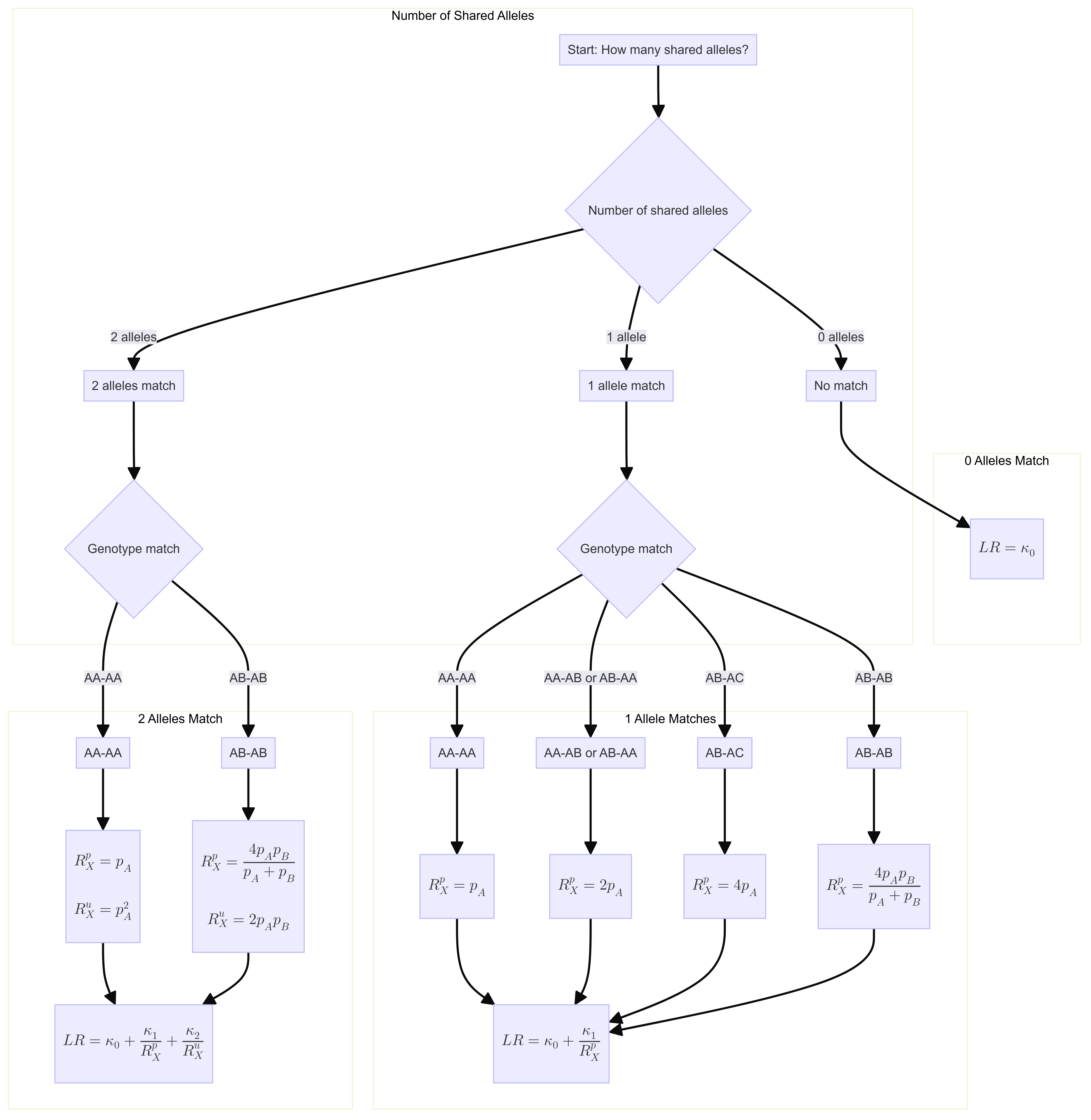
Likelihood ratio for a single locus is:
\[ R=\kappa_0+\kappa_1 / R_X^p+\kappa_2 / R_X^u \] Where \(\kappa\) is the probability of having 0, 1 or 2 alleles IBD for a given relationship.
The \(R_X\) terms are quantifying the “surprisingness” of a particular pattern of allele sharing.
The \(R_X^p\) terms attached to the \(kappa_1\) are defined in the following table:
\[ \begin{aligned} &\text { Table 7.2 Single-locus LRs for paternity when } \mathcal{C}_M \text { is unavailable. }\\ &\begin{array}{llc} \hline c & Q & R_X \times\left(1+2 F_{S T}\right) \\ \hline \mathrm{AA} & \mathrm{AA} & 3 F_{S T}+\left(1-F_{S T}\right) p_A \\ \mathrm{AA} & \mathrm{AB} & 2\left(2 F_{S T}+\left(1-F_{S T}\right) p_A\right) \\ \mathrm{AB} & \mathrm{AA} & 2\left(2 F_{S T}+\left(1-F_{S T}\right) p_A\right) \\ \mathrm{AB} & \mathrm{AC} & 4\left(F_{S T}+\left(1-F_{S T}\right) p_A\right) \\ \mathrm{AB} & \mathrm{AB} & 4\left(F_{S T}+\left(1-F_{S T}\right) p_A\right)\left(F_{S T}+\left(1-F_{S T}\right) p_B\right) /\left(2 F_{S T}+\left(1-F_{S T}\right)\left(p_A+p_B\right)\right) \\ \hline \end{array} \end{aligned} \]
For our purposes we will take out the \(F_{S T}\) values. So the table will be as follows:
\[ \begin{aligned} &\begin{array}{llc} \hline c & Q & R_X \\ \hline \mathrm{AA} & \mathrm{AA} & p_A \\ \mathrm{AA} & \mathrm{AB} & 2 p_A \\ \mathrm{AB} & \mathrm{AA} & 2p_A \\ \mathrm{AB} & \mathrm{AC} & 4p_A \\ \mathrm{AB} & \mathrm{AB} & 4 p_A p_B/(p_A+p_B) \\ \hline \end{array} \end{aligned} \]
If none of the alleles match, then the \(\kappa_1 / R_X^p = 0\).
The \(R_X^u\) terms attached to the \(kappa_2\) are defined as:
If both alleles match and are homozygous the equation is 6.4 (pg 85). Single locus match probability: \(\mathrm{CSP}=\mathcal{G}_Q=\mathrm{AA}\) \[ \frac{\left(2 F_{S T}+\left(1-F_{S T}\right) p_A\right)\left(3 F_{S T}+\left(1-F_{S T}\right) p_A\right)}{\left(1+F_{S T}\right)\left(1+2 F_{S T}\right)} \] Simplified to: \[ p_A{ }^2 \]
If both alleles match and are heterozygous, the equation is 6.5 (pg 85) Single locus match probability: \(\mathrm{CSP}=\mathcal{G}_Q=\mathrm{AB}\) \[ 2 \frac{\left(F_{S T}+\left(1-F_{S T}\right) p_A\right)\left(F_{S T}+\left(1-F_{S T}\right) p_B\right)}{\left(1+F_{S T}\right)\left(1+2 F_{S T}\right)} \] Simplified to:
\[ 2 p_A p_B \] If both alleles do not match then \(\kappa_2 / R_X^u = 0\).
LR function
Flowchart
 ## Likelihood ratio funtion
calculate_likelihood_ratio <- function(shared_alleles, genotype_match = NULL, pA = NULL, pB = NULL, k0, k1, k2) {

  # Case 0: No Shared Alleles
  if (shared_alleles == 0) {
    LR <- k0
    return(LR)
  }

  # Case 1: One Shared Allele
  if (shared_alleles == 1) {
    if (genotype_match == "AA-AA") {
      Rxp <- pA
    } else if (genotype_match == "AA-AB" | genotype_match == "AB-AA") {
      Rxp <- 2 * pA
    } else if (genotype_match == "AB-AC") {
      Rxp <- 4 * pA
    } else if (genotype_match == "AB-AB") {
      Rxp <- (4 * pA * pB) / (pA + pB)
    } else {
      stop("Invalid genotype match for 1 shared allele.")
    }

    LR <- k0 + (k1 / Rxp)
    return(LR)
  }

  # Case 2: Two Shared Alleles
  if (shared_alleles == 2) {
    if (genotype_match == "AA-AA") {
      Rxp <- pA
      Rxu <- pA^2
    } else if (genotype_match == "AB-AB") {
      Rxp <- (4 * pA * pB) / (pA + pB)
      Rxu <- 2 * pA * pB
    } else {
      stop("Invalid genotype match for 2 shared alleles.")
    }

    LR <- k0 + (k1 / Rxp) + (k2 / Rxu)
    return(LR)
  }
}
Input for LR function
Rscript for simulation
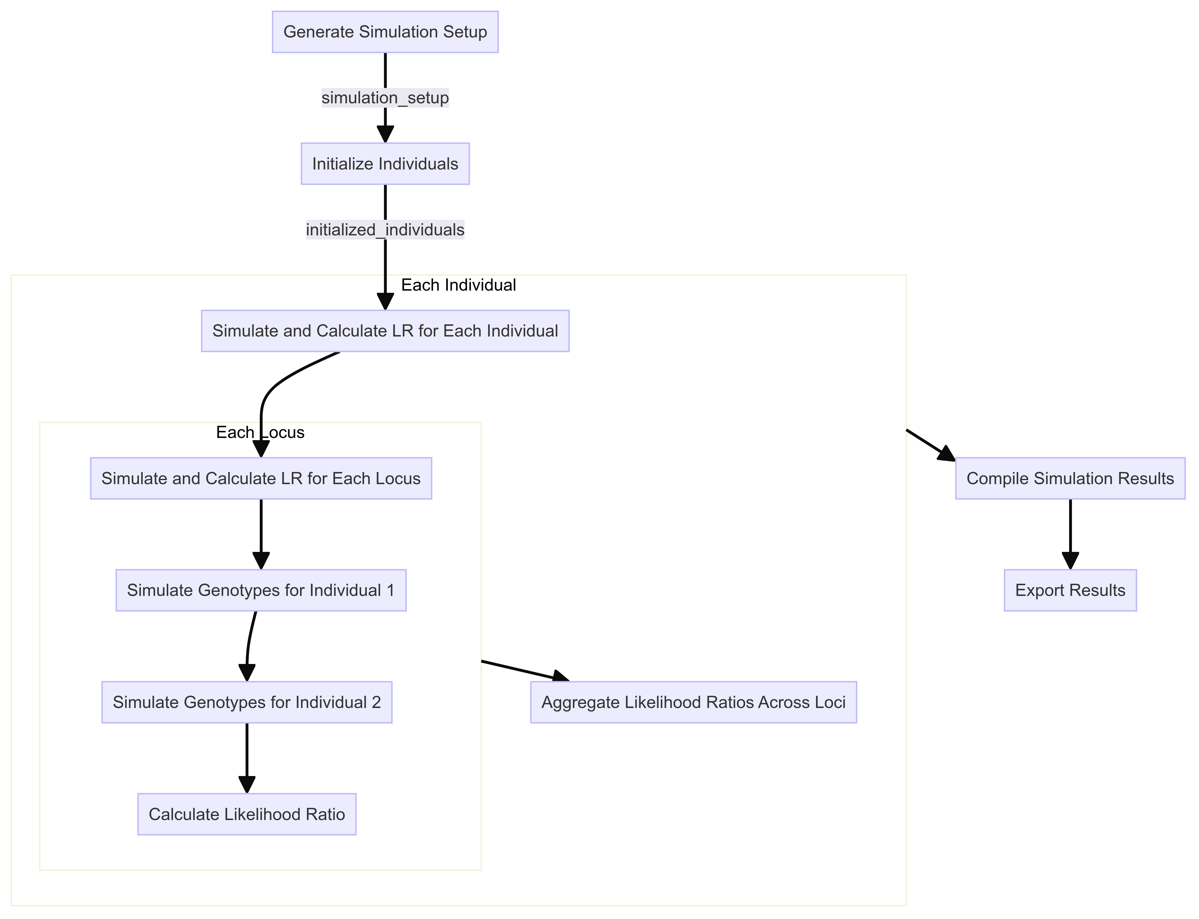
Step 1: Simulation Setup
The first step is to set up the simulation by defining the parameters and functions required for generating the simulated data. This includes specifying the population size, allele frequencies, and the kinship matrix for likelihood ratio calculations. The simulation will generate pairs of individuals with known relationships (e.g., parent-child, siblings) and unknown relationships (unrelated) based on the specified parameters.
generate_simulation_setup <- function(kinship_matrix, population_list, num_related, num_unrelated) {
  # Create an empty dataframe to store the simulation setup
  simulation_setup <- data.frame(
    population = character(),
    relationship_type = character(),
    num_simulations = integer(),
    stringsAsFactors = FALSE
  )

  # Loop through each population and relationship type to create the setup
  for (population in population_list) {
    for (relationship in kinship_matrix$relationship_type) {
      num_simulations <- ifelse(relationship == "unrelated", num_unrelated, num_related)

      # Append to the simulation setup dataframe
      simulation_setup <- rbind(simulation_setup, data.frame(
        population = population,
        relationship_type = relationship,
        num_simulations = num_simulations
      ))
    }
  }

  return(simulation_setup)
}
The necessary parameters for this are initialized beforehand.
First, the kinship coefficients are provided in a matrix:
# Create a dataframe with relationship types and their respective kinship coefficients (k0, k1, k2)
kinship_matrix <- tibble(
    relationship_type =
      c("parent_child", "full_siblings", "half_siblings", "cousins", "second_cousins", "unrelated"),
    k0 = c(0, 1/4, 1/2, 7/8, 15/16, 1),
    k1 = c(1, 1/2, 1/2, 1/8, 1/16, 0),
    k2 = c(0, 1/4, 0, 0, 0, 0)
  )

# Print the kinship matrix to check the contents
print(kinship_matrix)
# A tibble: 6 × 4
relationship_type k0 k1 k2
<chr> <dbl> <dbl> <dbl>
1 parent_child 0 1 0
2 full_siblings 0.25 0.5 0.25
3 half_siblings 0.5 0.5 0
4 cousins 0.875 0.125 0
5 second_cousins 0.938 0.0625 0
6 unrelated 1 0 0 Then a list of populations is created:
[1] "all" "AfAm" "Cauc" "Hispanic" "Asian" Now we can test the simulation setup function:### Step 1: Simulation Setup
The first step is to set up the simulation by defining the parameters and functions required for generating the simulated data. This includes specifying the population size, allele frequencies, and the kinship matrix for likelihood ratio calculations. The simulation will generate pairs of individuals with known relationships (e.g., parent-child, siblings) and unknown relationships (unrelated) based on the specified parameters.
generate_simulation_setup <- function(kinship_matrix, population_list, num_related, num_unrelated) {
  # Create an empty dataframe to store the simulation setup
  simulation_setup <- data.frame(
    population = character(),
    relationship_type = character(),
    num_simulations = integer(),
    stringsAsFactors = FALSE
  )

  # Loop through each population and relationship type to create the setup
  for (population in population_list) {
    for (relationship in kinship_matrix$relationship_type) {
      num_simulations <- ifelse(relationship == "unrelated", num_unrelated, num_related)

      # Append to the simulation setup dataframe
      simulation_setup <- rbind(simulation_setup, data.frame(
        population = population,
        relationship_type = relationship,
        num_simulations = num_simulations
      ))
    }
  }

  return(simulation_setup)
}
The necessary parameters for this are initialized beforehand.
First, the kinship coefficients are provided in a matrix:
# Create a dataframe with relationship types and their respective kinship coefficients (k0, k1, k2)
kinship_matrix <- tibble(
    relationship_type =
      c("parent_child", "full_siblings", "half_siblings", "cousins", "second_cousins", "unrelated"),
    k0 = c(0, 1/4, 1/2, 7/8, 15/16, 1),
    k1 = c(1, 1/2, 1/2, 1/8, 1/16, 0),
    k2 = c(0, 1/4, 0, 0, 0, 0)
  )

# Print the kinship matrix to check the contents
print(kinship_matrix)
# A tibble: 6 × 4
relationship_type k0 k1 k2
<chr> <dbl> <dbl> <dbl>
1 parent_child 0 1 0
2 full_siblings 0.25 0.5 0.25
3 half_siblings 0.5 0.5 0
4 cousins 0.875 0.125 0
5 second_cousins 0.938 0.0625 0
6 unrelated 1 0 0 Then a list of populations is created:
[1] "all" "AfAm" "Cauc" "Hispanic" "Asian" Now we can test the simulation setup function:
   population relationship_type num_simulations
1         all      parent_child               2
2         all     full_siblings               2
3         all     half_siblings               2
4         all           cousins               2
5         all    second_cousins               2
6         all         unrelated               5
7        AfAm      parent_child               2
8        AfAm     full_siblings               2
9        AfAm     half_siblings               2
10       AfAm           cousins               2
11       AfAm    second_cousins               2
12       AfAm         unrelated               5
13       Cauc      parent_child               2
14       Cauc     full_siblings               2
15       Cauc     half_siblings               2
16       Cauc           cousins               2
17       Cauc    second_cousins               2
18       Cauc         unrelated               5
19   Hispanic      parent_child               2
20   Hispanic     full_siblings               2
21   Hispanic     half_siblings               2
22   Hispanic           cousins               2
23   Hispanic    second_cousins               2
24   Hispanic         unrelated               5
25      Asian      parent_child               2
26      Asian     full_siblings               2
27      Asian     half_siblings               2
28      Asian           cousins               2
29      Asian    second_cousins               2
30      Asian         unrelated               5
Step 2: Initialize Individuals
Once the general simulation setup is done, each pair of individuals must be initialized as its own dataframe. This requires knowing how many loci will be simulated per pair. We will therefore first extract the unique loci from our allele frequency tables.
Rows: 387 Columns: 4
── Column specification ────────────────────────────────────────────────────────
Delimiter: ","
chr (2): marker, population
dbl (2): allele, frequency

ℹ Use `spec()` to retrieve the full column specification for this data.
ℹ Specify the column types or set `show_col_types = FALSE` to quiet this message.
Rows: 453 Columns: 4
── Column specification ────────────────────────────────────────────────────────
Delimiter: ","
chr (2): marker, population
dbl (2): allele, frequency

ℹ Use `spec()` to retrieve the full column specification for this data.
ℹ Specify the column types or set `show_col_types = FALSE` to quiet this message.
Rows: 277 Columns: 4
── Column specification ────────────────────────────────────────────────────────
Delimiter: ","
chr (2): marker, population
dbl (2): allele, frequency

ℹ Use `spec()` to retrieve the full column specification for this data.
ℹ Specify the column types or set `show_col_types = FALSE` to quiet this message.
Rows: 344 Columns: 4
── Column specification ────────────────────────────────────────────────────────
Delimiter: ","
chr (2): marker, population
dbl (2): allele, frequency

ℹ Use `spec()` to retrieve the full column specification for this data.
ℹ Specify the column types or set `show_col_types = FALSE` to quiet this message.
Rows: 348 Columns: 4
── Column specification ────────────────────────────────────────────────────────
Delimiter: ","
chr (2): marker, population
dbl (2): allele, frequency

ℹ Use `spec()` to retrieve the full column specification for this data.
ℹ Specify the column types or set `show_col_types = FALSE` to quiet this message.
# A tibble: 1,809 × 4
marker allele frequency population
<chr> <dbl> <dbl> <chr>
1 Penta_D 2.2 0.114 AfAm
2 F13A01 3.2 0.118 AfAm
3 Penta_D 3.2 0.00877 AfAm
4 F13A01 4 0.0687 AfAm
5 F13A01 4.2 0.00146 AfAm
6 D16S539 5 0.00146 AfAm
7 F13A01 5 0.339 AfAm
8 Penta_C 5 0.0249 AfAm
9 Penta_D 5 0.0439 AfAm
10 Penta_E 5 0.0950 AfAm
# ℹ 1,799 more rowsWe will now extract the unique loci from the allele frequency tables:
 [1] "Penta_D"  "F13A01"   "D16S539"  "Penta_C"  "Penta_E"  "TH01"
 [7] "D7S820"   "F13B"     "FESFPS"   "TPOX"     "CSF1PO"   "D5S818"
[13] "LPL"      "SE33"     "D10S1248" "D13S317"  "D22S1045" "D8S1179"
[19] "D18S51"   "D2S441"   "D6S1043"  "D19S433"  "D1S1656"  "vWA"
[25] "D3S1358"  "D12S391"  "D2S1338"  "FGA"      "D21S11"
Number of unique loci: 29 These are the 29 autosomal loci from the 2013 and 2017 FSI paper on US STR allele frequencies for 29 autosomal STR loci Steffen et al 2017.
We will use the list of different required loci to calculate likelihood ratios for pairs of individuals. Below is a reference with which loci are used in various sets.
      locus core_13 identifiler_15 expanded_20 supplementary
1    CSF1PO       1              1           1             1
2       FGA       1              1           1             1
3      THO1       1              1           1             1
4      TPOX       1              1           1             1
5       vWA       1              1           1             1
6   D3S1358       1              1           1             1
7    D5S818       1              1           1             1
8    D7S820       1              1           1             1
9   D8S1179       1              1           1             1
10  D13S317       1              1           1             1
11  D16S539       1              1           1             1
12   D18S51       1              1           1             1
13   D21S11       1              1           1             1
14  D1S1656       0              0           1             1
15   D2S441       0              0           1             1
16  D2S1338       0              1           1             1
17 D10S1248       0              0           1             1
18  D12S391       0              0           1             1
19  D19S433       0              1           1             1
20 D22S1045       0              0           1             1
21     SE33       0              0           0             1
22  Penta_E       0              0           0             1
23  Penta_D       0              0           0             1
$core_13
[1] "CSF1PO" "FGA" "THO1" "TPOX" "vWA" "D3S1358" "D5S818"
[8] "D7S820" "D8S1179" "D13S317" "D16S539" "D18S51" "D21S11"
$identifiler_15
[1] "CSF1PO" "FGA" "THO1" "TPOX" "vWA" "D3S1358" "D5S818"
[8] "D7S820" "D8S1179" "D13S317" "D16S539" "D18S51" "D21S11" "D2S1338"
[15] "D19S433"
$expanded_20
[1] "CSF1PO" "FGA" "THO1" "TPOX" "vWA" "D3S1358"
[7] "D5S818" "D7S820" "D8S1179" "D13S317" "D16S539" "D18S51"
[13] "D21S11" "D1S1656" "D2S441" "D2S1338" "D10S1248" "D12S391"
[19] "D19S433" "D22S1045"
$supplementary
[1] "CSF1PO" "FGA" "THO1" "TPOX" "vWA" "D3S1358"
[7] "D5S818" "D7S820" "D8S1179" "D13S317" "D16S539" "D18S51"
[13] "D21S11" "D1S1656" "D2S441" "D2S1338" "D10S1248" "D12S391"
[19] "D19S433" "D22S1045" "SE33" "Penta_E" "Penta_D"
$autosomal_29
[1] "Penta_D" "F13A01" "D16S539" "Penta_C" "Penta_E" "TH01"
[7] "D7S820" "F13B" "FESFPS" "TPOX" "CSF1PO" "D5S818"
[13] "LPL" "SE33" "D10S1248" "D13S317" "D22S1045" "D8S1179"
[19] "D18S51" "D2S441" "D6S1043" "D19S433" "D1S1656" "vWA"
[25] "D3S1358" "D12S391" "D2S1338" "FGA" "D21S11" Now we can initialize the individuals:
[1] "Initialized individuals:" population relationship_type sim_id locus ind1_allele1 ind1_allele2
1 all parent_child 1 Penta_D
2 all parent_child 1 F13A01
3 all parent_child 1 D16S539
4 all parent_child 1 Penta_C
5 all parent_child 1 Penta_E
6 all parent_child 1 TH01
7 all parent_child 1 D7S820
8 all parent_child 1 F13B
9 all parent_child 1 FESFPS
10 all parent_child 1 TPOX
11 all parent_child 1 CSF1PO
12 all parent_child 1 D5S818
13 all parent_child 1 LPL
14 all parent_child 1 SE33
15 all parent_child 1 D10S1248
16 all parent_child 1 D13S317
17 all parent_child 1 D22S1045
18 all parent_child 1 D8S1179
19 all parent_child 1 D18S51
20 all parent_child 1 D2S441
21 all parent_child 1 D6S1043
22 all parent_child 1 D19S433
23 all parent_child 1 D1S1656
24 all parent_child 1 vWA
25 all parent_child 1 D3S1358
26 all parent_child 1 D12S391
27 all parent_child 1 D2S1338
28 all parent_child 1 FGA
29 all parent_child 1 D21S11
ind2_allele1 ind2_allele2 shared_alleles genotype_match LR
1 0 0
2 0 0
3 0 0
4 0 0
5 0 0
6 0 0
7 0 0
8 0 0
9 0 0
10 0 0
11 0 0
12 0 0
13 0 0
14 0 0
15 0 0
16 0 0
17 0 0
18 0 0
19 0 0
20 0 0
21 0 0
22 0 0
23 0 0
24 0 0
25 0 0
26 0 0
27 0 0
28 0 0
29 0 0Step 3: Simulate Genotypes
Step 4: Calculate Kinship
  population relationship_type sim_id  locus ind1_allele1 ind1_allele2
9        all      parent_child      1 FESFPS           11         10.3
  ind2_allele1 ind2_allele2 shared_alleles genotype_match LR
9         10.3           13              0                 0
population relationship_type sim_id locus ind1_allele1 ind1_allele2
9 all parent_child 1 FESFPS 11 10.3
ind2_allele1 ind2_allele2 shared_alleles genotype_match LR
9 10.3 13 1 AB-AC 16.70968 population relationship_type sim_id locus ind1_allele1 ind1_allele2
1 all parent_child 1 Penta_D 13 12
2 all parent_child 1 F13A01 7 5
3 all parent_child 1 D16S539 9 12
4 all parent_child 1 Penta_C 14 11
5 all parent_child 1 Penta_E 11 13
6 all parent_child 1 TH01 6 7
7 all parent_child 1 D7S820 11 9
8 all parent_child 1 F13B 10 10
9 all parent_child 1 FESFPS 12 11
10 all parent_child 1 TPOX 6 8
11 all parent_child 1 CSF1PO 10 10
12 all parent_child 1 D5S818 10 13
13 all parent_child 1 LPL 10 11
14 all parent_child 1 SE33 25.2 17
15 all parent_child 1 D10S1248 13 14
16 all parent_child 1 D13S317 11 12
17 all parent_child 1 D22S1045 15 17
18 all parent_child 1 D8S1179 16 12
19 all parent_child 1 D18S51 15 13
20 all parent_child 1 D2S441 12 14
21 all parent_child 1 D6S1043 13 19
22 all parent_child 1 D19S433 15 14
23 all parent_child 1 D1S1656 16.3 16
24 all parent_child 1 vWA 14 17
25 all parent_child 1 D3S1358 17 18
26 all parent_child 1 D12S391 16 17
27 all parent_child 1 D2S1338 19 22
28 all parent_child 1 FGA 22 18
29 all parent_child 1 D21S11 30.2 29
ind2_allele1 ind2_allele2 shared_alleles genotype_match LR
1 13 8 1 AB-AC 1.8031359
2 5 6 1 AB-AC 1.0882353
3 11 12 1 AB-AC 0.9736842
4 13 11 1 AB-AC 0.7485549
5 14 13 1 AB-AC 2.7700535
6 9 6 1 AB-AC 1.2758621
7 11 9 2 AB-AB 3.1213992
8 9 10 1 AA-AB 1.4428969
9 12 11 2 AB-AB 1.7009816
10 11 6 1 AB-AC 7.8409091
11 12 10 1 AA-AB 2.1538462
12 13 12 1 AB-AC 1.5325444
13 11 11 1 AB-AA 2.6361323
14 17 29.2 1 AB-AC 3.4078947
15 13 13 1 AB-AA 1.8080279
16 11 11 1 AB-AA 1.7209302
17 15 15 1 AB-AA 1.5578947
18 15 16 1 AB-AC 5.1287129
19 13 12 1 AB-AC 2.3870968
20 14 12 2 AB-AB 3.6166908
21 12 13 1 AB-AC 2.5643564
22 15 15 1 AB-AA 4.2459016
23 17.3 16.3 1 AB-AC 3.6737589
24 17 15 1 AB-AC 0.9539595
25 18 16 1 AB-AC 2.3652968
26 16 18 1 AB-AC 6.1666667
27 20 19 1 AB-AC 1.6818182
28 23 22 1 AB-AC 1.2665037
29 31 29 1 AB-AC 1.2245863Execution time for list_of_rows_approach: user system elapsed
0.546 0.013 1.460 Execution time for future_pmap_approach: user system elapsed
0.506 0.007 0.542 Benchmark results for both approaches:Unit: milliseconds
expr min lq mean median uq max neval
list_of_rows 540.2258 549.6349 557.7970 554.4797 569.1483 577.8931 10
future_pmap 540.2387 544.3072 552.3609 548.7928 553.6963 577.4973 10 population relationship_type num_simulations
1 all parent_child 2
2 all full_siblings 2
3 all half_siblings 2
4 all cousins 2
5 all second_cousins 2
6 all unrelated 5
7 AfAm parent_child 2
8 AfAm full_siblings 2
9 AfAm half_siblings 2
10 AfAm cousins 2
11 AfAm second_cousins 2
12 AfAm unrelated 5
13 Cauc parent_child 2
14 Cauc full_siblings 2
15 Cauc half_siblings 2
16 Cauc cousins 2
17 Cauc second_cousins 2
18 Cauc unrelated 5
19 Hispanic parent_child 2
20 Hispanic full_siblings 2
21 Hispanic half_siblings 2
22 Hispanic cousins 2
23 Hispanic second_cousins 2
24 Hispanic unrelated 5
25 Asian parent_child 2
26 Asian full_siblings 2
27 Asian half_siblings 2
28 Asian cousins 2
29 Asian second_cousins 2
30 Asian unrelated 5Step 2: Initialize Individuals
Once the general simulation setup is done, each pair of individuals must be initialized as its own dataframe. This requires knowing how many loci will be simulated per pair. We will therefore first extract the unique loci from our allele frequency tables.
Rows: 387 Columns: 4
── Column specification ────────────────────────────────────────────────────────
Delimiter: ","
chr (2): marker, population
dbl (2): allele, frequency

ℹ Use `spec()` to retrieve the full column specification for this data.
ℹ Specify the column types or set `show_col_types = FALSE` to quiet this message.
Rows: 453 Columns: 4
── Column specification ────────────────────────────────────────────────────────
Delimiter: ","
chr (2): marker, population
dbl (2): allele, frequency

ℹ Use `spec()` to retrieve the full column specification for this data.
ℹ Specify the column types or set `show_col_types = FALSE` to quiet this message.
Rows: 277 Columns: 4
── Column specification ────────────────────────────────────────────────────────
Delimiter: ","
chr (2): marker, population
dbl (2): allele, frequency

ℹ Use `spec()` to retrieve the full column specification for this data.
ℹ Specify the column types or set `show_col_types = FALSE` to quiet this message.
Rows: 344 Columns: 4
── Column specification ────────────────────────────────────────────────────────
Delimiter: ","
chr (2): marker, population
dbl (2): allele, frequency

ℹ Use `spec()` to retrieve the full column specification for this data.
ℹ Specify the column types or set `show_col_types = FALSE` to quiet this message.
Rows: 348 Columns: 4
── Column specification ────────────────────────────────────────────────────────
Delimiter: ","
chr (2): marker, population
dbl (2): allele, frequency

ℹ Use `spec()` to retrieve the full column specification for this data.
ℹ Specify the column types or set `show_col_types = FALSE` to quiet this message.
# A tibble: 1,809 × 4
marker allele frequency population
<chr> <dbl> <dbl> <chr>
1 Penta_D 2.2 0.114 AfAm
2 F13A01 3.2 0.118 AfAm
3 Penta_D 3.2 0.00877 AfAm
4 F13A01 4 0.0687 AfAm
5 F13A01 4.2 0.00146 AfAm
6 D16S539 5 0.00146 AfAm
7 F13A01 5 0.339 AfAm
8 Penta_C 5 0.0249 AfAm
9 Penta_D 5 0.0439 AfAm
10 Penta_E 5 0.0950 AfAm
# ℹ 1,799 more rowsWe will now extract the unique loci from the allele frequency tables:
 [1] "Penta_D"  "F13A01"   "D16S539"  "Penta_C"  "Penta_E"  "TH01"
 [7] "D7S820"   "F13B"     "FESFPS"   "TPOX"     "CSF1PO"   "D5S818"
[13] "LPL"      "SE33"     "D10S1248" "D13S317"  "D22S1045" "D8S1179"
[19] "D18S51"   "D2S441"   "D6S1043"  "D19S433"  "D1S1656"  "vWA"
[25] "D3S1358"  "D12S391"  "D2S1338"  "FGA"      "D21S11"
Number of unique loci: 29 These are the 29 autosomal loci from the 2013 and 2017 FSI paper on US STR allele frequencies for 29 autosomal STR loci Steffen et al 2017.
We will use the list of different required loci to calculate likelihood ratios for pairs of individuals. Below is a reference with which loci are used in various sets.
      locus core_13 identifiler_15 expanded_20 supplementary
1    CSF1PO       1              1           1             1
2       FGA       1              1           1             1
3      THO1       1              1           1             1
4      TPOX       1              1           1             1
5       vWA       1              1           1             1
6   D3S1358       1              1           1             1
7    D5S818       1              1           1             1
8    D7S820       1              1           1             1
9   D8S1179       1              1           1             1
10  D13S317       1              1           1             1
11  D16S539       1              1           1             1
12   D18S51       1              1           1             1
13   D21S11       1              1           1             1
14  D1S1656       0              0           1             1
15   D2S441       0              0           1             1
16  D2S1338       0              1           1             1
17 D10S1248       0              0           1             1
18  D12S391       0              0           1             1
19  D19S433       0              1           1             1
20 D22S1045       0              0           1             1
21     SE33       0              0           0             1
22  Penta_E       0              0           0             1
23  Penta_D       0              0           0             1
$core_13
[1] "CSF1PO" "FGA" "THO1" "TPOX" "vWA" "D3S1358" "D5S818"
[8] "D7S820" "D8S1179" "D13S317" "D16S539" "D18S51" "D21S11"
$identifiler_15
[1] "CSF1PO" "FGA" "THO1" "TPOX" "vWA" "D3S1358" "D5S818"
[8] "D7S820" "D8S1179" "D13S317" "D16S539" "D18S51" "D21S11" "D2S1338"
[15] "D19S433"
$expanded_20
[1] "CSF1PO" "FGA" "THO1" "TPOX" "vWA" "D3S1358"
[7] "D5S818" "D7S820" "D8S1179" "D13S317" "D16S539" "D18S51"
[13] "D21S11" "D1S1656" "D2S441" "D2S1338" "D10S1248" "D12S391"
[19] "D19S433" "D22S1045"
$supplementary
[1] "CSF1PO" "FGA" "THO1" "TPOX" "vWA" "D3S1358"
[7] "D5S818" "D7S820" "D8S1179" "D13S317" "D16S539" "D18S51"
[13] "D21S11" "D1S1656" "D2S441" "D2S1338" "D10S1248" "D12S391"
[19] "D19S433" "D22S1045" "SE33" "Penta_E" "Penta_D"
$autosomal_29
[1] "Penta_D" "F13A01" "D16S539" "Penta_C" "Penta_E" "TH01"
[7] "D7S820" "F13B" "FESFPS" "TPOX" "CSF1PO" "D5S818"
[13] "LPL" "SE33" "D10S1248" "D13S317" "D22S1045" "D8S1179"
[19] "D18S51" "D2S441" "D6S1043" "D19S433" "D1S1656" "vWA"
[25] "D3S1358" "D12S391" "D2S1338" "FGA" "D21S11" Now we can initialize the individuals:
[1] "Initialized individuals:" population relationship_type sim_id locus ind1_allele1 ind1_allele2
1 all parent_child 1 Penta_D
2 all parent_child 1 F13A01
3 all parent_child 1 D16S539
4 all parent_child 1 Penta_C
5 all parent_child 1 Penta_E
6 all parent_child 1 TH01
7 all parent_child 1 D7S820
8 all parent_child 1 F13B
9 all parent_child 1 FESFPS
10 all parent_child 1 TPOX
11 all parent_child 1 CSF1PO
12 all parent_child 1 D5S818
13 all parent_child 1 LPL
14 all parent_child 1 SE33
15 all parent_child 1 D10S1248
16 all parent_child 1 D13S317
17 all parent_child 1 D22S1045
18 all parent_child 1 D8S1179
19 all parent_child 1 D18S51
20 all parent_child 1 D2S441
21 all parent_child 1 D6S1043
22 all parent_child 1 D19S433
23 all parent_child 1 D1S1656
24 all parent_child 1 vWA
25 all parent_child 1 D3S1358
26 all parent_child 1 D12S391
27 all parent_child 1 D2S1338
28 all parent_child 1 FGA
29 all parent_child 1 D21S11
ind2_allele1 ind2_allele2 shared_alleles genotype_match LR
1 0 0
2 0 0
3 0 0
4 0 0
5 0 0
6 0 0
7 0 0
8 0 0
9 0 0
10 0 0
11 0 0
12 0 0
13 0 0
14 0 0
15 0 0
16 0 0
17 0 0
18 0 0
19 0 0
20 0 0
21 0 0
22 0 0
23 0 0
24 0 0
25 0 0
26 0 0
27 0 0
28 0 0
29 0 0Step 3: Simulate Genotypes
Step 4: Calculate Kinship
  population relationship_type sim_id  locus ind1_allele1 ind1_allele2
9        all      parent_child      1 FESFPS           11           10
  ind2_allele1 ind2_allele2 shared_alleles genotype_match LR
9            8           10              0                 0
population relationship_type sim_id locus ind1_allele1 ind1_allele2
9 all parent_child 1 FESFPS 11 10
ind2_allele1 ind2_allele2 shared_alleles genotype_match LR
9 8 10 1 AB-AC 1.097458 population relationship_type sim_id locus ind1_allele1 ind1_allele2
1 all parent_child 1 Penta_D 11 14
2 all parent_child 1 F13A01 5 5
3 all parent_child 1 D16S539 12 10
4 all parent_child 1 Penta_C 9 9
5 all parent_child 1 Penta_E 19 18
6 all parent_child 1 TH01 9 7
7 all parent_child 1 D7S820 11 11
8 all parent_child 1 F13B 10 8
9 all parent_child 1 FESFPS 12 11
10 all parent_child 1 TPOX 11 8
11 all parent_child 1 CSF1PO 10 10
12 all parent_child 1 D5S818 13 12
13 all parent_child 1 LPL 10 10
14 all parent_child 1 SE33 19 28.2
15 all parent_child 1 D10S1248 14 15
16 all parent_child 1 D13S317 8 12
17 all parent_child 1 D22S1045 16 12
18 all parent_child 1 D8S1179 14 13
19 all parent_child 1 D18S51 12 15
20 all parent_child 1 D2S441 10 11
21 all parent_child 1 D6S1043 12 12
22 all parent_child 1 D19S433 12 12
23 all parent_child 1 D1S1656 19.3 16
24 all parent_child 1 vWA 14 17
25 all parent_child 1 D3S1358 18 16
26 all parent_child 1 D12S391 17 19
27 all parent_child 1 D2S1338 25 20
28 all parent_child 1 FGA 21 23
29 all parent_child 1 D21S11 32.2 32.2
ind2_allele1 ind2_allele2 shared_alleles genotype_match LR
1 7 11 1 AB-AC 1.6071429
2 6 5 1 AA-AB 2.1764706
3 10 9 1 AB-AC 2.3125000
4 11 9 1 AA-AB 2.5900000
5 12 18 1 AB-AC 7.8484848
6 7 7 1 AB-AA 1.6955810
7 10 11 1 AA-AB 2.1316872
8 8 10 2 AB-AB 2.2056892
9 13 12 1 AB-AC 1.0614754
10 9 11 1 AB-AC 1.0227273
11 10 10 1 AA-AA 4.3076923
12 12 11 1 AB-AC 0.7076503
13 10 10 1 AA-AA 2.3125000
14 31.2 19 1 AB-AC 2.6839378
15 13 15 1 AB-AC 1.2422062
16 13 8 1 AB-AC 2.5900000
17 12 14 1 AB-AC 9.7735849
18 13 13 1 AB-AA 1.8633094
19 13 15 1 AB-AC 1.4971098
20 10 14 1 AB-AC 1.2304038
21 12 19 1 AA-AB 2.3333333
22 12 14.2 1 AA-AB 5.9884393
23 15 16 1 AB-AC 1.7559322
24 14 17 2 AB-AB 3.5701211
25 15 16 1 AB-AC 0.8839590
26 17 17 1 AB-AA 4.0155039
27 22 20 1 AB-AC 1.8836364
28 23 19 1 AB-AC 1.6037152
29 32.2 27 1 AA-AB 5.4814815Execution time for list_of_rows_approach: user system elapsed
0.528 0.009 1.450 Execution time for future_pmap_approach: user system elapsed
0.501 0.007 0.536 Benchmark results for both approaches:Unit: milliseconds
expr min lq mean median uq max neval
list_of_rows 526.1602 540.7774 547.7191 543.9689 560.0311 568.3521 10
future_pmap 526.1298 541.5628 558.2019 548.1681 583.6142 589.4595 10`summarise()` has grouped output by 'population', 'relationship_type'. You can
override using the `.groups` argument.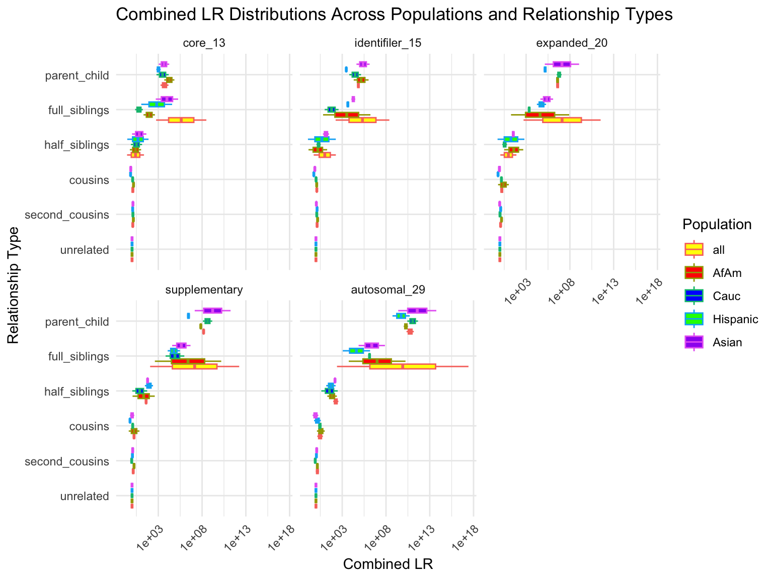
`summarise()` has grouped output by 'relationship_type', 'population'. You can
override using the `.groups` argument.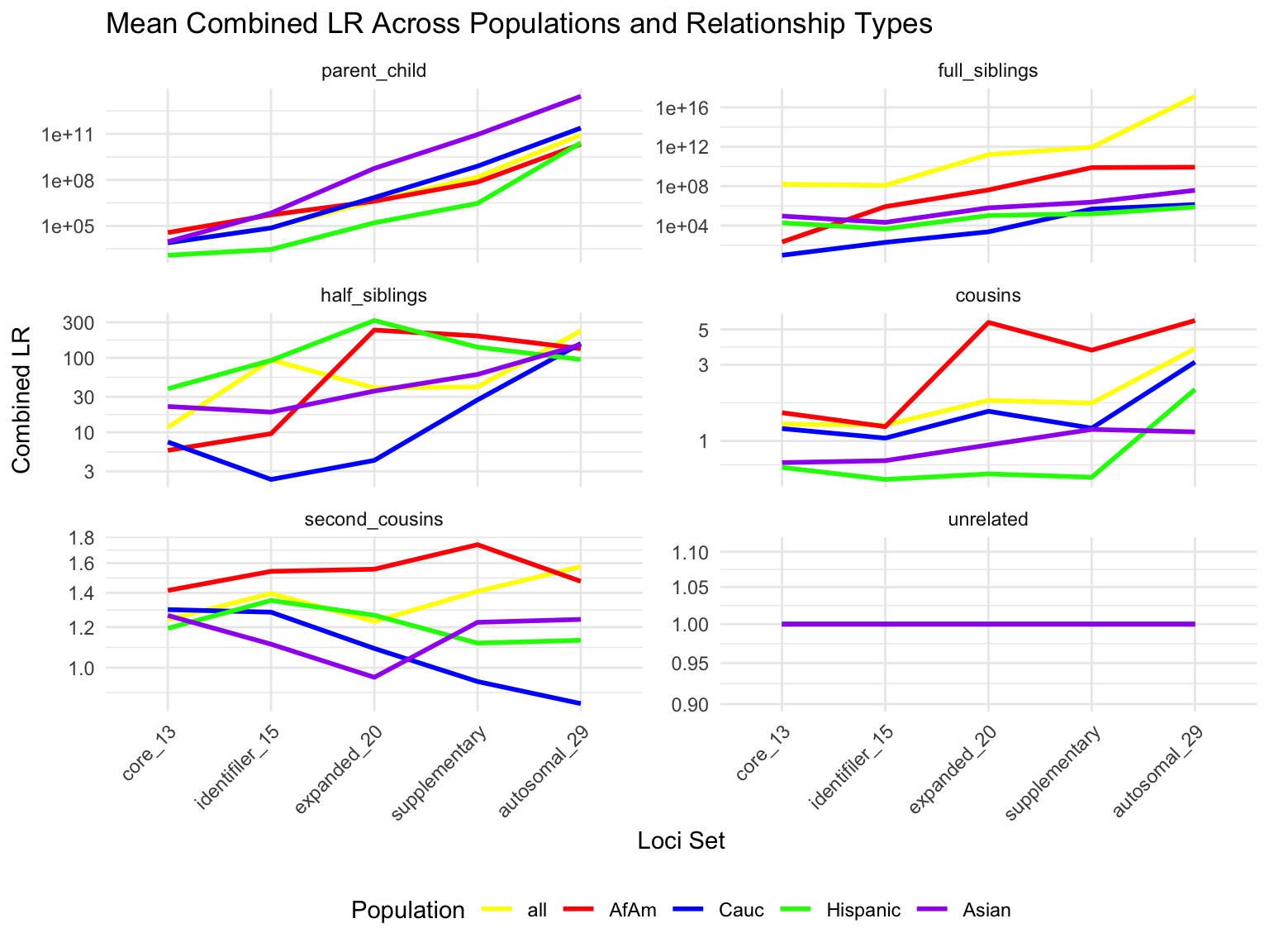
# A tibble: 5 × 5
  loci_set       fixed_cutoff cutoff_1 cutoff_0_1 cutoff_0_01
  <fct>                 <dbl>    <dbl>      <dbl>       <dbl>
1 core_13                   1        1          1           1
2 identifiler_15            1        1          1           1
3 expanded_20               1        1          1           1
4 supplementary             1        1          1           1
5 autosomal_29              1        1          1           1
# A tibble: 125 × 7
population relationship_type loci_set proportion_exceeding_fixed
<fct> <fct> <fct> <dbl>
1 all parent_child core_13 1
2 all parent_child identifiler_15 1
3 all parent_child expanded_20 1
4 all parent_child supplementary 1
5 all parent_child autosomal_29 1
6 all full_siblings core_13 1
7 all full_siblings identifiler_15 1
8 all full_siblings expanded_20 1
9 all full_siblings supplementary 1
10 all full_siblings autosomal_29 1
# ℹ 115 more rows
# ℹ 3 more variables: proportion_exceeding_1 <dbl>,
# proportion_exceeding_0_1 <dbl>, proportion_exceeding_0_01 <dbl>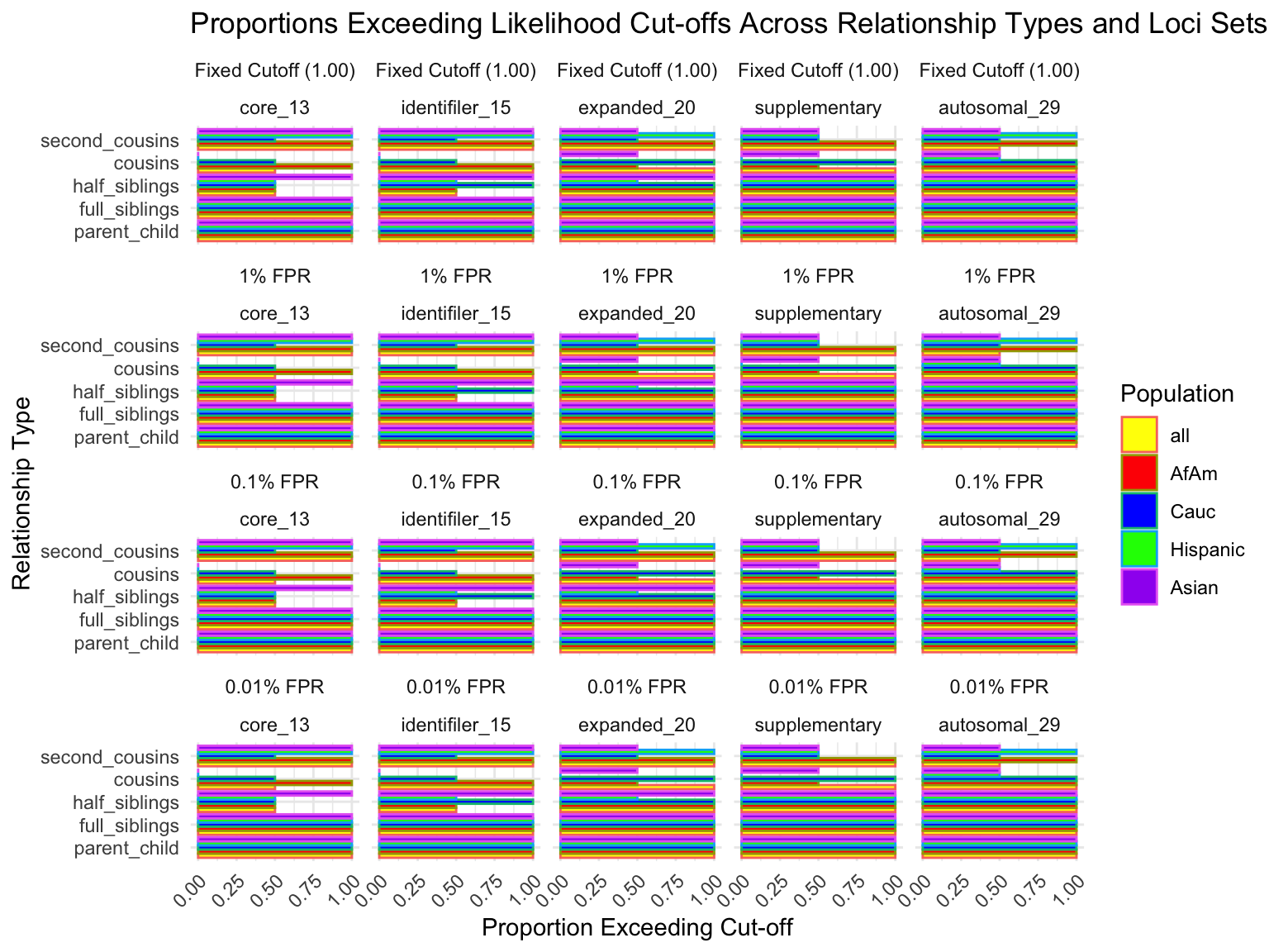
Simulation results
Rows: 360000 Columns: 6
── Column specification ────────────────────────────────────────────────────────
Delimiter: ","
chr (3): population, known_relationship_type, tested_relationship_type
dbl (3): replicate_id, num_shared_alleles_sum, log_R_sum
ℹ Use `spec()` to retrieve the full column specification for this data.
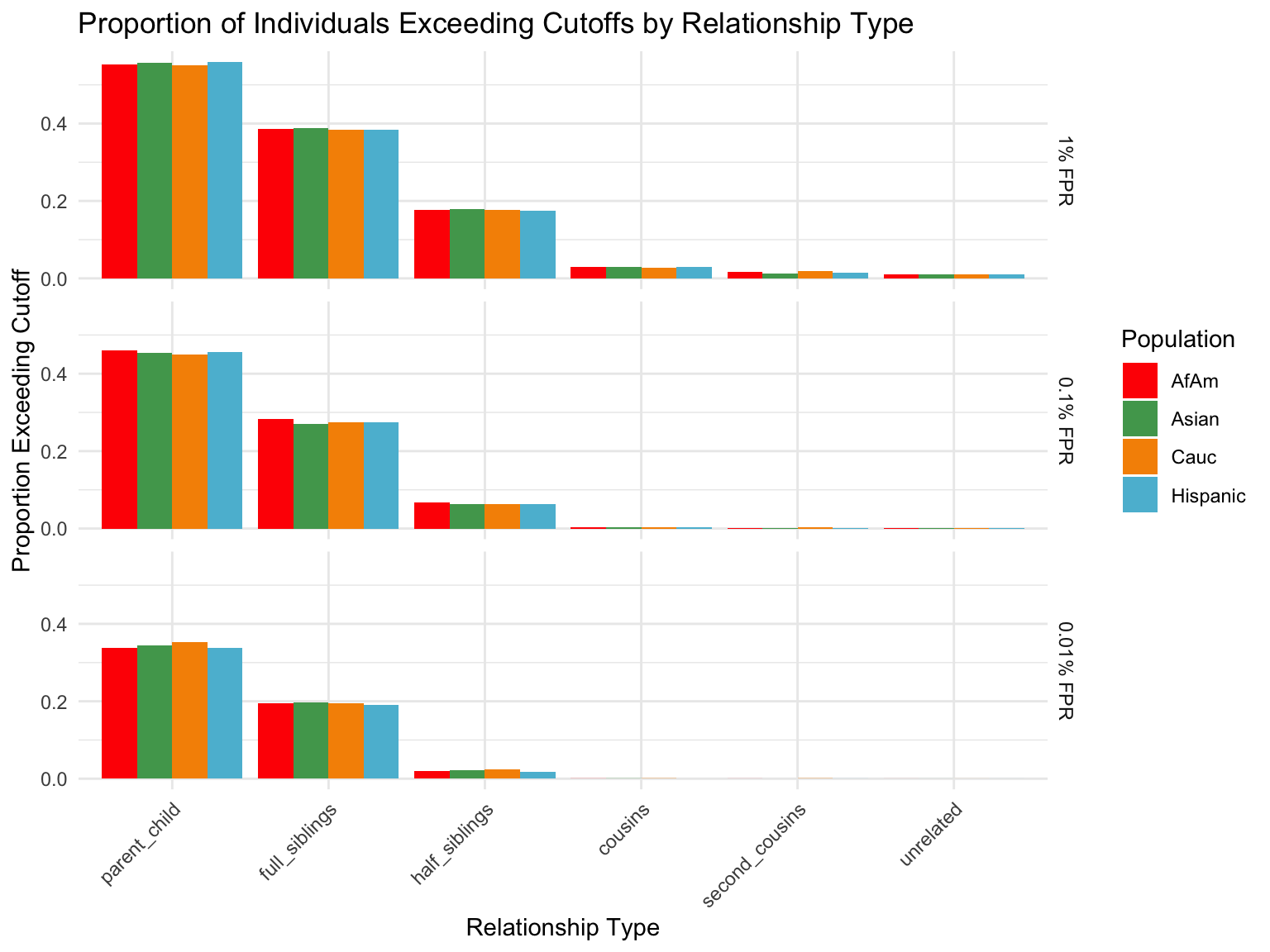
ℹ Specify the column types or set `show_col_types = FALSE` to quiet this message.Proportion of individuals of known relationship type exceeding likelihood cut-off
  population relationship_type fp_rate prop_exceeding
1       AfAm      parent_child     0.1          1.000
2      Asian      parent_child     0.1          1.000
3       Cauc      parent_child     0.1          1.000
4   Hispanic      parent_child     0.1          1.000
5       AfAm     full_siblings     0.1          0.794
6      Asian     full_siblings     0.1          0.820
`summarise()` has grouped output by 'population'. You can override using the
`.groups` argument.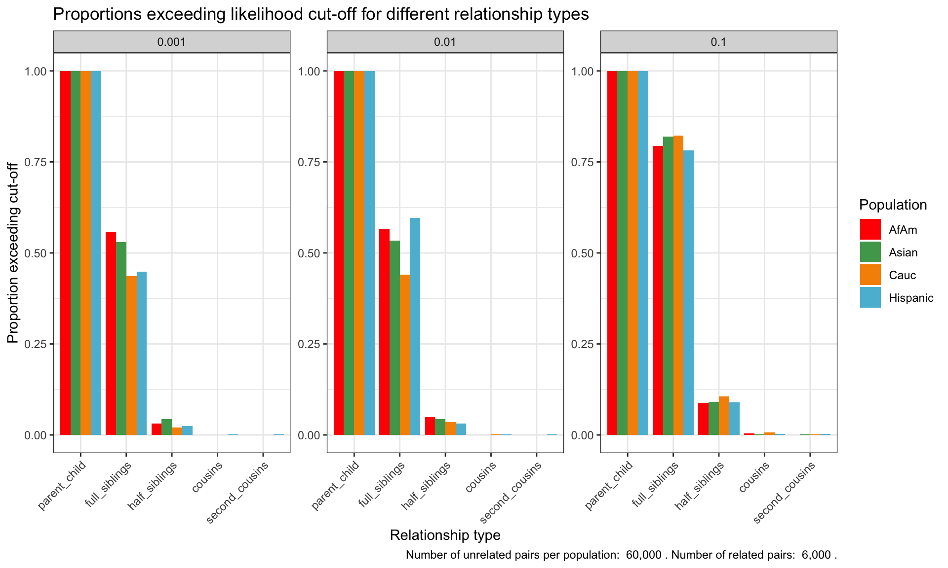
Cut-offs for each FPR
`summarise()` has grouped output by 'population'. You can override using the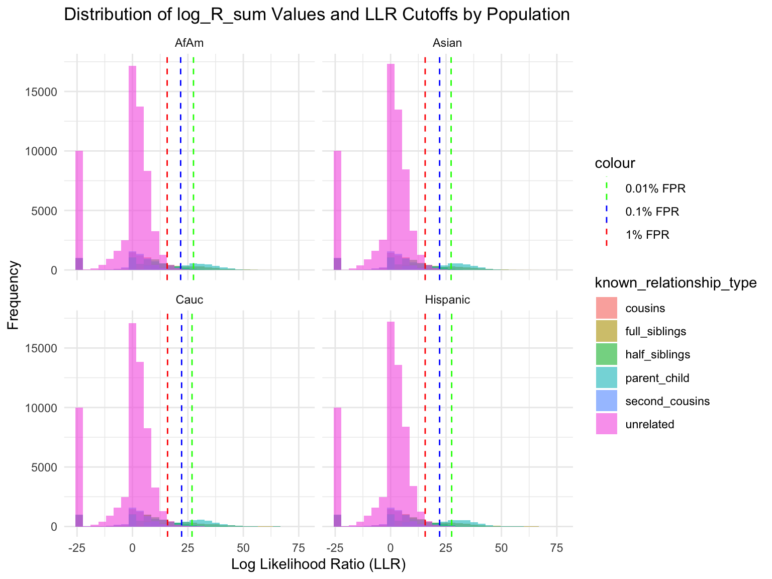
`.groups` argument.# A tibble: 24 × 7
population known_relationship_type mean_log_R_sum median_log_R_sum
<chr> <chr> <dbl> <dbl>
1 AfAm cousins -0.533 2.42
2 AfAm full_siblings 10.5 11.5
3 AfAm half_siblings 3.85 6.80
4 AfAm parent_child 19.6 19.0
5 AfAm second_cousins -1.23 1.78
6 AfAm unrelated -2.00 0.914
7 Asian cousins -0.538 2.42
8 Asian full_siblings 10.5 11.6
9 Asian half_siblings 3.82 6.78
10 Asian parent_child 19.5 18.9
# ℹ 14 more rows
# ℹ 3 more variables: min_log_R_sum <dbl>, max_log_R_sum <dbl>, count <int>Calculate LLR cutoffs for unrelated pairs at each FPR by population
This table presents aggregated log_R_sum values by relationship type for each population, alongside LLR cutoffs calculated for unrelated pairs to maintain false positive rates (FPRs) of 1%, 0.1%, and 0.01%. The cutoffs indicate the LLR threshold above which a pair is less likely to be unrelated at the given FPR, thereby serving as a critical benchmark for assessing relationship evidence. The mean log_R_sum values further elucidate the average strength of genetic evidence supporting each relationship type within populations, highlighting variations and consistencies in genetic relatedness indicators across demographic groups.
| population | cousins | full_siblings | half_siblings | parent_child | second_cousins | unrelated |
|---|---|---|---|---|---|---|
| AfAm | -0.5334790 | 10.45417 | 3.849582 | 19.62211 | -1.229432 | -2.003701 |
| Asian | -0.5379709 | 10.45853 | 3.821000 | 19.54267 | -1.387000 | -1.982983 |
| Cauc | -0.5075911 | 10.48275 | 3.873924 | 19.51039 | -1.218428 | -1.982207 |
| Hispanic | -0.5536143 | 10.40972 | 3.837237 | 19.58039 | -1.249979 | -1.984905 |
R version 4.4.1 (2024-06-14)
Platform: x86_64-apple-darwin20
Running under: macOS Sonoma 14.5

Matrix products: default
BLAS:   /Library/Frameworks/R.framework/Versions/4.4-x86_64/Resources/lib/libRblas.0.dylib
LAPACK: /Library/Frameworks/R.framework/Versions/4.4-x86_64/Resources/lib/libRlapack.dylib;  LAPACK version 3.12.0

locale:
[1] en_US.UTF-8/en_US.UTF-8/en_US.UTF-8/C/en_US.UTF-8/en_US.UTF-8

time zone: America/Detroit
tzcode source: internal

attached base packages:
[1] stats     graphics  grDevices utils     datasets  methods   base

other attached packages:
 [1] furrr_0.3.1           future_1.33.2         kableExtra_1.4.0
 [4] microbenchmark_1.4.10 patchwork_1.2.0       lubridate_1.9.3
 [7] forcats_1.0.0         stringr_1.5.1         dplyr_1.1.4
[10] purrr_1.0.2           readr_2.1.5           tidyr_1.3.1
[13] tibble_3.2.1          ggplot2_3.5.1         tidyverse_2.0.0
[16] RColorBrewer_1.1-3    wesanderson_0.3.7     workflowr_1.7.1

loaded via a namespace (and not attached):
 [1] gtable_0.3.5      xfun_0.45         bslib_0.7.0       processx_3.8.4
 [5] callr_3.7.6       tzdb_0.4.0        vctrs_0.6.5       tools_4.4.1
 [9] ps_1.7.6          generics_0.1.3    parallel_4.4.1    fansi_1.0.6
[13] highr_0.11        pkgconfig_2.0.3   lifecycle_1.0.4   farver_2.1.2
[17] compiler_4.4.1    git2r_0.33.0      textshaping_0.4.0 munsell_0.5.1
[21] codetools_0.2-20  getPass_0.2-4     httpuv_1.6.15     htmltools_0.5.8.1
[25] sass_0.4.9        yaml_2.3.8        crayon_1.5.3      later_1.3.2
[29] pillar_1.9.0      jquerylib_0.1.4   whisker_0.4.1     cachem_1.1.0
[33] parallelly_1.37.1 tidyselect_1.2.1  digest_0.6.36     stringi_1.8.4
[37] listenv_0.9.1     labeling_0.4.3    rprojroot_2.0.4   fastmap_1.2.0
[41] grid_4.4.1        colorspace_2.1-0  cli_3.6.3         magrittr_2.0.3
[45] utf8_1.2.4        withr_3.0.0       scales_1.3.0      promises_1.3.0
[49] bit64_4.0.5       timechange_0.3.0  rmarkdown_2.27    httr_1.4.7
[53] globals_0.16.3    bit_4.0.5         ragg_1.3.2        hms_1.1.3
[57] evaluate_0.24.0   knitr_1.47        viridisLite_0.4.2 rlang_1.1.4
[61] Rcpp_1.0.12       glue_1.7.0        xml2_1.3.6        vroom_1.6.5
[65] svglite_2.1.3     rstudioapi_0.16.0 jsonlite_1.8.8    R6_2.5.1
[69] systemfonts_1.1.0 fs_1.6.4