Log
Last updated: 2020-11-16
Checks: 7 0
Knit directory: GradLog/
This reproducible R Markdown analysis was created with workflowr (version 1.6.2). The Checks tab describes the reproducibility checks that were applied when the results were created. The Past versions tab lists the development history.
Great! Since the R Markdown file has been committed to the Git repository, you know the exact version of the code that produced these results.
Great job! The global environment was empty. Objects defined in the global environment can affect the analysis in your R Markdown file in unknown ways. For reproduciblity it’s best to always run the code in an empty environment.
The command set.seed(20201014) was run prior to running the code in the R Markdown file. Setting a seed ensures that any results that rely on randomness, e.g. subsampling or permutations, are reproducible.
Great job! Recording the operating system, R version, and package versions is critical for reproducibility.
Nice! There were no cached chunks for this analysis, so you can be confident that you successfully produced the results during this run.
Great job! Using relative paths to the files within your workflowr project makes it easier to run your code on other machines.
Great! You are using Git for version control. Tracking code development and connecting the code version to the results is critical for reproducibility.
The results in this page were generated with repository version 7266ca3. See the Past versions tab to see a history of the changes made to the R Markdown and HTML files.
Note that you need to be careful to ensure that all relevant files for the analysis have been committed to Git prior to generating the results (you can use wflow_publish or wflow_git_commit). workflowr only checks the R Markdown file, but you know if there are other scripts or data files that it depends on. Below is the status of the Git repository when the results were generated:
Ignored files:
    Ignored:    .DS_Store
    Ignored:    .Rhistory
    Ignored:    .Rproj.user/
    Ignored:    analysis/.DS_Store
    Ignored:    code/.DS_Store
    Ignored:    data/.DS_Store
    Ignored:    output/.DS_Store

Untracked files:
    Untracked:  data/signals.summary.txt
Note that any generated files, e.g. HTML, png, CSS, etc., are not included in this status report because it is ok for generated content to have uncommitted changes.
These are the previous versions of the repository in which changes were made to the R Markdown (analysis/Log.Rmd) and HTML (docs/Log.html) files. If you’ve configured a remote Git repository (see ?wflow_git_remote), click on the hyperlinks in the table below to view the files as they were in that past version.
| File | Version | Author | Date | Message |
|---|---|---|---|---|
| Rmd | 7266ca3 | Lili Wang | 2020-11-16 | For Nov 06 |
| html | 7266ca3 | Lili Wang | 2020-11-16 | For Nov 06 |
| html | f0a14c6 | Lili Wang | 2020-11-05 | Build site. |
| Rmd | 58f14e8 | Lili Wang | 2020-11-05 | wflow_publish(“analysis/Log.Rmd”) |
| html | 58f14e8 | Lili Wang | 2020-11-05 | wflow_publish(“analysis/Log.Rmd”) |
| Rmd | 5bc34ec | Lili Wang | 2020-11-03 | Build site. |
| html | 5bc34ec | Lili Wang | 2020-11-03 | Build site. |
| Rmd | 8fe4184 | Lili Wang | 2020-11-03 | Build site. |
| html | 8fe4184 | Lili Wang | 2020-11-03 | Build site. |
Nov 16
Work I did.
For the last week, I re-write the whole pipeline into snakemake files, so that I can run different datasets with ease. script
Before listing the results, I will first describe the key steps in the pipeine.
- Construct co-expressed modules using
minModuleSize=20. - Compute zscores by tensorQTL.
- Compute pvalues by TruncPCO.
- Adjust for multiple testing based on one-time permutation, followed by Bonferroni.
Results summary.
This table is for the results summary.
Warning in read.table(file = file, header = header, sep = sep, quote = quote, :
incomplete final line found by readTableHeader on 'data/signals.summary.txt'| Dataset | nGene | nModule | pvalue | pvalue correction | FDR level | “(transeQTL, module)” | unique transeQTLs | independent transeQTLs |
|---|---|---|---|---|---|---|---|---|
| TCGA | 17673;8963;8710 | 81 | TruncPCO | empirical null | 0.05 | 17210 | 17171 | 2063 |
| DGN | 11979; 8120; 3859 | 21 | TruncPCO | empirical null | 0.05 | 3536 | 3439 | 500 |
TCGA
The following plot is for the 2063 independent signals. The left plot is the histogram of \(-logp\). Since signals with \(p<10^{-16}\) have pvalue as 0 in R, here I give these signals pvalue of \(10^{-17}\), which have \(-logp=17\). The plot shows that among 2063 signals, most of them have \(p \approx 10^{-5}\).
Question: Is this too small for claiming significance for trans?
The right plot is the histogram of the chromosomes the signals are on.

DGN
As showed in the plot for DGN, among 500 independent signals, most of their pvalues have \(p \approx 10^{-5}\).

GTEx
- Expression data pre-process.
Below is how GTEx 2020 paper pre-processs expression data.
“Gene-level expression quantification was performed using RNA-SeQC [68]. Gene-level read counts and TPM values were produced using the following read-level filters: 1) reads were uniquely mapped (corresponding to a mapping quality of 255 for STAR BAMs); 2) reads were aligned in proper pairs; 3) the read alignment distance was ≤ 6; 4) reads were fully contained within exon boundaries. Reads overlapping introns were not counted. These filters were applied using the “-strictMode” flag in RNA-SeQC. Gene expression values for all samples from a given tissue were normalized for eQTL analyses using the following procedure: 1) read counts were normalized between samples using TMM [69]; 2) genes were selected based on expression thresholds of ≥0.1 TPM in ≥20% of samples and ≥6 reads (unnormalized) in ≥20% of samples; 3) expression values for each gene were inverse normal transformed across samples." link
- Genotype data pre-process.
Any filter? QCed? script?
Nov 09
Paper using permutation-based false discovery rate.
This paper uses permutations to correct for FDR of a complex test statistic. Like in our cases, it’s unrealistic to do thousands of permutations. Specifically, they did 10 permutations and adjusted pvalues based on these 10 empirical null distributions. They justied why 10 permutations are enough.
Modify PCO code from one SNP a time to multiple SNPs.
- davies method
davies.R: Remove PACKAGE=MPAT; Run in command line R SMP SHLIB qfc.cpp; Run in R dyn.load("./script/qfc.so")
- liumod method
Use liumod method when p.WI ==0 | p.WI < 0.
Snakemake pipeline.
Results
z (tensorQTL) + p (TruncPCO) + FDR (one time permutation).
z & p: add index for observe data or permutation.
minModuleSize=20 in WGCNA.
DGN; TCGA
Nov 02
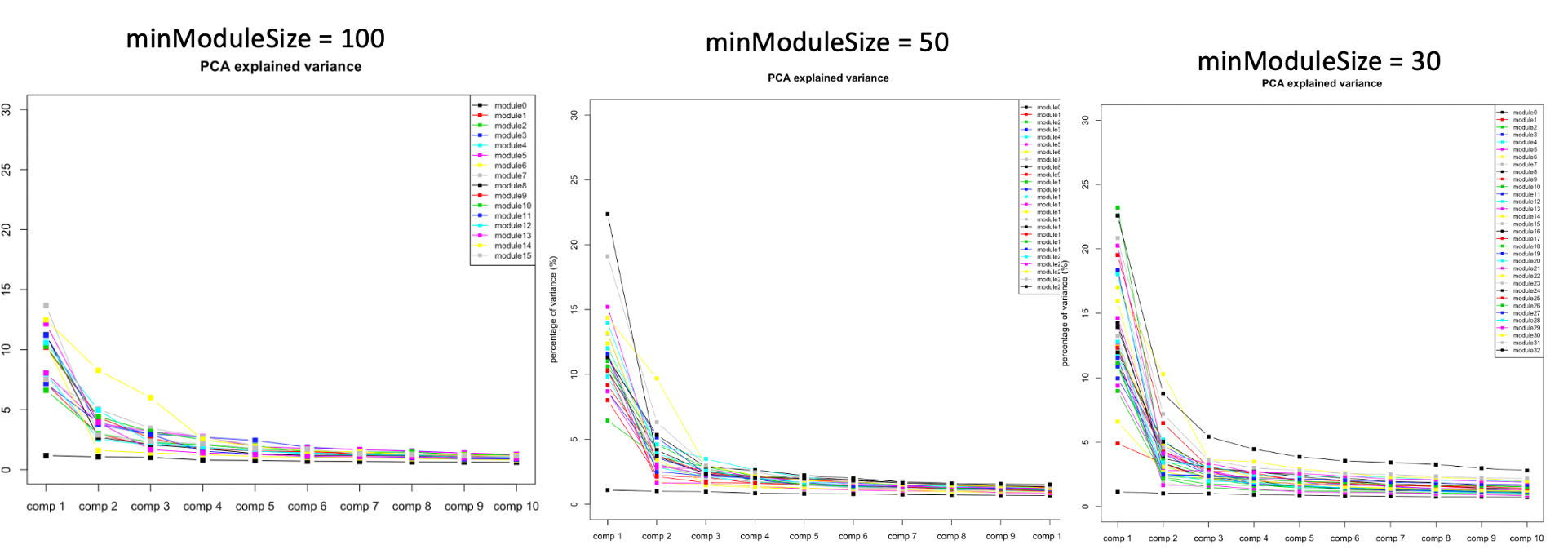
Why use minModuleSize=30 in WGCNA for TCGA?
There are three reasons why I set the minimum number of genes in modules to be 30.
1. DGN used this setting.
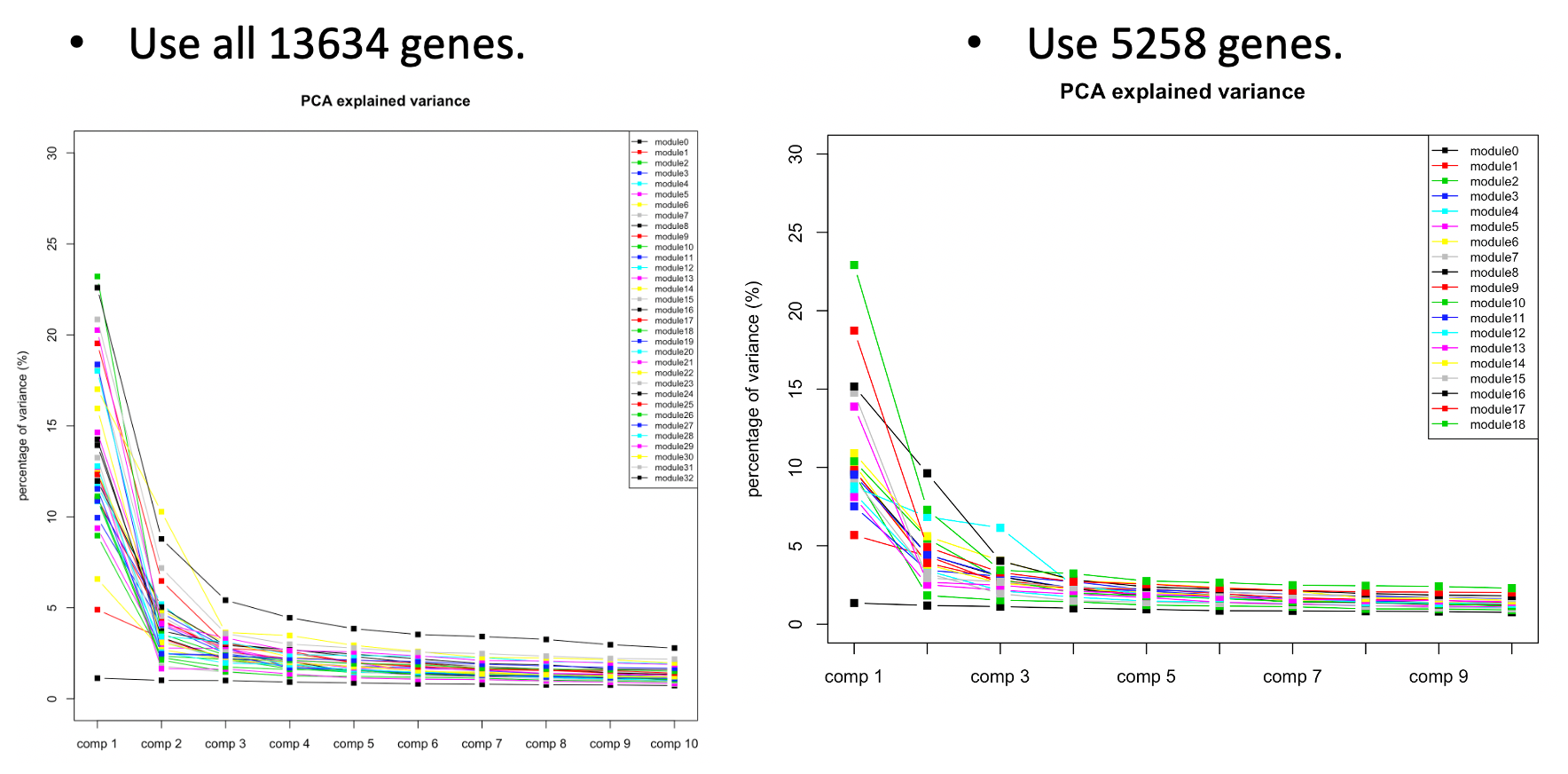
At first, we looked at the variance explained by the top three PC of each modules under different settings, i.e. minModuleSize=100, 50, 30. We found that under setting of 30, the top three PC’s explained more variance, so we tended to use 30.
| Version | Author | Date |
|---|---|---|
| 8fe4184 | Lili Wang | 2020-11-03 |
The above plots used all 13634 genes without removing any poorly mapped genes. Next, I removed the poorly mapped genes, with 5258 genes left. I used 30 to cluster these 5258 genes and resulted in 18 modules. We then looked at the explained variance and found nothing seemed wrong. So we decided to use 30 for WGCNA and these 18 modules for downstream analysis.
| Version | Author | Date |
|---|---|---|
| 8fe4184 | Lili Wang | 2020-11-03 |
2. 30 is the default module size in WGCNA tutorial, and also used by the elife paper.
WGCNA tutorial used 30 as default. The elife method also used the default parameters. (Correction: elife method used the default parameters in the R package, where minClusterSize = 20.)
3. I tried other parameters, e.g. 100. 50, which both increase the unclassified genes.
| minModuleSize | Num.unclassified.genes | Num.modules | Max.num.genes |
|---|---|---|---|
| 100 | 5247 | 4 | 1972 |
| 50 | 3251 | 33 | 397 |
| 30 | 2908 | 57 | 356 |
| 20 | 2813 | 81 | 326 |
Look into enrichment of TCGA modules.
Here is the complete enrichment result.
KEGG pathway enrichment
| source | term_name | sig_module | p_adjusted |
|---|---|---|---|
| KEGG | ErbB signaling pathway | 21 | 0.008964903 |
| KEGG | Neuroactive ligand-receptor interaction | 3 | 0.015524997 |
| KEGG | Mucin type O-glycan biosynthesis | 20 | 0.016931426 |
| KEGG | Human papillomavirus infection | 2 | 0.019400355 |
| KEGG | Prolactin signaling pathway | 2 | 0.041320205 |
| KEGG | Cocaine addiction | 2;26 | 0.04269822;0.049447144 |
| KEGG | PI3K-Akt signaling pathway | 21 | 0.048894331 |
ErbB signaling pathway: "ErbB family members and some of their ligands are often over-expressed, amplified, or mutated in many forms of cancer, making them important therapeutic targets. For example, researchers have found EGFR to be amplified and/or mutated in gliomas and NSCLC while ErbB2 amplifications are seen in breast, ovarian, bladder, NSCLC, as well as several other tumor types. [source]
Neuroactive ligand-receptor interaction:
Mucin type O-glycan biosynthesis: “Changes in mucin-type O-linked glycosylation are seen in over 90% of breast cancers” [source] [source]
Human papillomavirus infection: “We demonstrated that HPV is associated with breast cancer development, although the role of HPV in breast cancers is still questionable and further research is required to investigate, in more detail, the role of HPV infection in breast cancer.” [source]
Prolactin signaling pathway: “elevated PRL levels are correlated with increased breast cancer risk and metastasis” “In vitro studies have indicated a role for PRL in breast cancer proliferation and survival.” [source]
Cocaine addiction: ???
PI3K-Akt signaling pathway: “PI3K/Akt signaling pathway is key in the development of BC” (breast cancer) [source]
Debug code for TruncPCO.
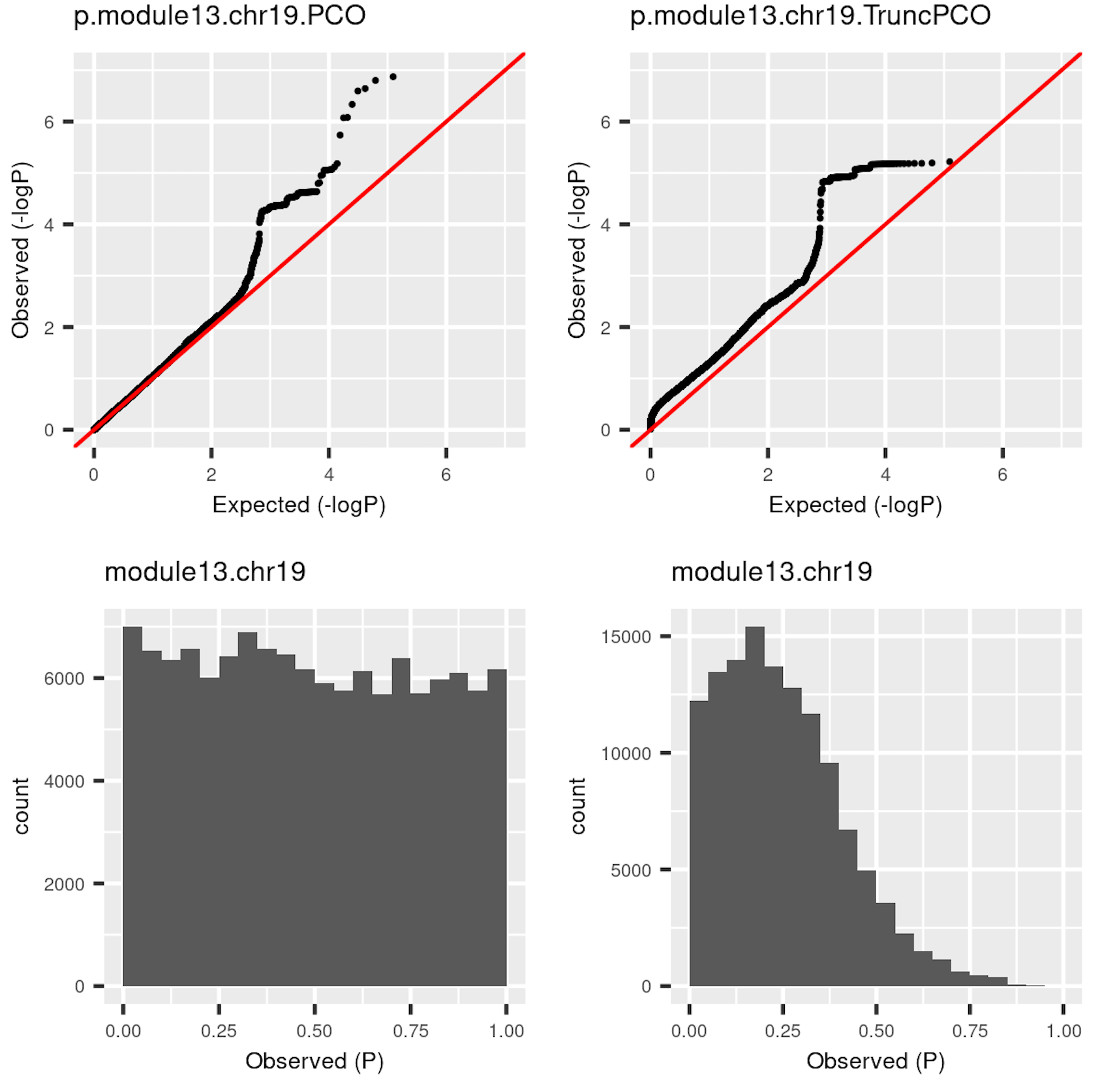
I was doubting that TruncPCO (using only \(\lambda>1\)) code may have bugs because of the following weird qqplot and histogram of pvalues.
| Version | Author | Date |
|---|---|---|
| 58f14e8 | Lili Wang | 2020-11-05 |
Rows are qqplot and histogram of pvalues. These pvalues are observed pvalues rather than null pvalues. Left column is for standard PCO (using all \(\lambda\)’s); right is for TruncPCO. I thought TruncPCO is weird because a histogram of pvalues shouldn’t be as skewed as the lower right one. This skewed plot means pvalues by TruncPCO are overall smaller than PCO. We thought this may be due to LD among snps, i.e. the tests are not independent. However, even with the LD complication, the histogram should be approximately flat as in the lower left plot, where the tests are not independent either.
So I looked into the code for TruncPCO and see if there are bugs I didn’t notice. (This paragraph explains what the bug is. See the histogram by the debugged code in next paragraph.) PCO uses the minimum pvalue of six tests as the test statistic, i.e. \[T_{PCO}=min(p_{PCMinP}, p_{PCFisher}, p_{PCLC}, p_{WI}, p_{Wald}, p_{VC})\]
Then use a inverse normal distribution to calculate pvalue of \(T_{PCO}\). So the key step is to compute the six pvalues. The bug happens in the step of computing \(p_{WI}\). The test statistic for this pvalus is, \[T_{WI}=\sum_{k=1}^K {z_k^2} = \sum_{k=1}^K {PC_k^2}=\sum_{k=1}^K {\lambda_k \chi_{1k}^2}\] ,where \(K\) is number of all PC’s of expression matrix, \(PC_k=u_k^Tz \sim N(0, \lambda_k)\), \(u_k\) is k-th eigenvector with eigenvalue \(\lambda_k\); \(z\) is zscore vector for one snp to \(K\) genes, \(\chi_{1k}\) is chi-square distribution with DF 1. If we only use \(\lambda>1\) for TruncPCO, i.e. \(T_{WI}^{Trunc}=\sum_{k=1}^{k_0} {PC_k^2}=\sum_{k=1}^{k_0} {\lambda_k \chi_{1k}^2}\), what I only need to do is to subset \(\lambda\)’s and \(PC_k\)’s. That is what I did for other five tests. However, in the original PCO package, \(T_{WI}\) is calculated using \(\sum_{k=1}^K {z_k^2}\) and I should have changed \(z_k\)’s to \(PC_k\)’s. But I missed this. So, \(T_{WI}\) actually used all \(K\) \(z_k\)’s, and it’s larger than the real \(T_{WI}^{Trunc}\), therefore the pvalue is smaller than the real \(p_{WI}^{Trunc}\). That is why in the above plot, TruncPCO has many small pvalues and its histogram skews to the left.
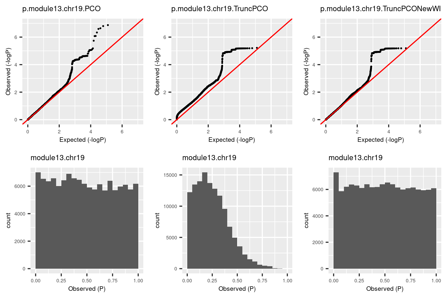
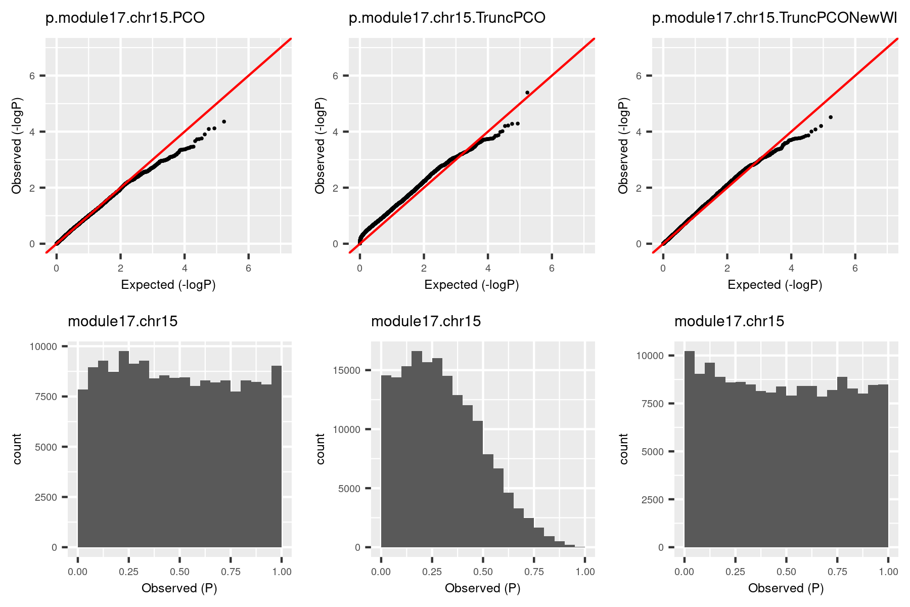
So I used the debuged code and re-computed pvalues for the same (module, chr). The result is in the third column.
| Version | Author | Date |
|---|---|---|
| 58f14e8 | Lili Wang | 2020-11-05 |
The histogram became approximately flat. For this (module13, chr19), there seems to be some signals. Next, I give another example (module, chr), where there seems no signals.
| Version | Author | Date |
|---|---|---|
| 58f14e8 | Lili Wang | 2020-11-05 |
The histogram by the debugged TruncPCO is still almost flat in this cese, which makes sense.
Now I have the updated pvalues. Next, I rerun TruncPCO for the null zscore, and use the null p’s to adjust for these updated pvalues. Then see how many snps are significant (\(p_{adj}<\frac{0.05}{18\times22}\)). I do this because I want to see how are the signals by this debugged TruncPCO compared with those by the previous TruncPCO. For now, I checked for the above two (module, chr) and the signals are almost the same.
From now on, I will use this correct version of TruncPCO to compute p’s for other datasets and update p’s for datasets I’ve analyzed.
Use tensorQTL do more permutation?
So far, the way we use to adjust p is to permute samples once, calculate null z, then null p, then using this null p distribution to adjust the observe p’s. This one-time permutation procedure should work. We do the permutation once because multiple permutation is computation-time heavy. So can we use tensorQTL to make permutation faster?
As far as I understand, tensorQTL is like FastQTL, which does fast permutation to provide the adjusted minimum pvalues for each gene. This is gene-level adjustment, not the snp-level adjustment as we want. So we can’t have more faster permutations by tensorQTL.
Do another round of permutation.
To see how stable the signals are, I do another round of permutation for the above two (module, chr). Here I use TruncPCO for pvalues and empirical null for p adjustment. The following table gives the results.
| example | oldTruncPCO.perm.1 | TruncPCO.perm.1 | TruncPCO.perm.2 |
|---|---|---|---|
| (module13,chr19) | 157 | 159 | 155 |
| (module17,chr15) | 1 | 0 | 1 |
Notation table
To make it clear, the following table is for notations of different methods.
| data | PCO | TruncPCO.old | TruncPCO |
|---|---|---|---|
| observe | p.PCO | NA | p.TruncPCO |
| null | p.null.PCO | NA | p.null.TruncPCO |
- “data” is for the data used. “observe” means pvalues are calculated from the observed data. “null” means pvalues are computed from permutation data. This is needed because we need to adjust pvalues in the downstream FDR analysis using the empirical null distribution of pvalues.
- We use empirical null because snps are in LD, so the tests are not independent and therefore the null distribution of p is not necessarily uniform.
- Why not using BH? BH assumes independent tests and uniform null.
- Why not using Bonferroni? Conservative for snp-level FDR correction, particularly for the trans snp-level FDR.
Approaches to deal with the multiple testing in QTL studies, cis and trans. (???)
- “PCO” is the standard PCO using all \(\lambda\)’s. “TruncPCO.old” is PCO using only \(\lambda>1\). This is the method used for all results obtained before 11/02/2020. I added “.old” because the code of this TruncPCO has bugs. “TruncPCO” uses the debugded code.
Signals we have so far.
| Version | Author | Date |
|---|---|---|
| 58f14e8 | Lili Wang | 2020-11-05 |
R version 3.6.3 (2020-02-29)
Platform: x86_64-apple-darwin15.6.0 (64-bit)
Running under: macOS Catalina 10.15.6

Matrix products: default
BLAS:   /Library/Frameworks/R.framework/Versions/3.6/Resources/lib/libRblas.0.dylib
LAPACK: /Library/Frameworks/R.framework/Versions/3.6/Resources/lib/libRlapack.dylib

locale:
[1] en_US.UTF-8/en_US.UTF-8/en_US.UTF-8/C/en_US.UTF-8/en_US.UTF-8

attached base packages:
[1] stats     graphics  grDevices utils     datasets  methods   base

other attached packages:
[1] workflowr_1.6.2

loaded via a namespace (and not attached):
 [1] Rcpp_1.0.4      rprojroot_1.3-2 digest_0.6.25   later_1.0.0
 [5] R6_2.4.1        backports_1.1.5 git2r_0.27.1    magrittr_1.5
 [9] evaluate_0.14   highr_0.8       stringi_1.4.6   rlang_0.4.7
[13] fs_1.3.2        promises_1.1.0  whisker_0.4     rmarkdown_2.1
[17] tools_3.6.3     stringr_1.4.0   glue_1.3.2      httpuv_1.5.2
[21] xfun_0.12       yaml_2.2.1      compiler_3.6.3  htmltools_0.4.0
[25] knitr_1.28