Log2021
Last updated: 2021-06-29
Checks: 7 0
Knit directory: GradLog/
This reproducible R Markdown analysis was created with workflowr (version 1.6.2). The Checks tab describes the reproducibility checks that were applied when the results were created. The Past versions tab lists the development history.
Great! Since the R Markdown file has been committed to the Git repository, you know the exact version of the code that produced these results.
Great job! The global environment was empty. Objects defined in the global environment can affect the analysis in your R Markdown file in unknown ways. For reproduciblity it’s best to always run the code in an empty environment.
The command set.seed(20201014) was run prior to running the code in the R Markdown file. Setting a seed ensures that any results that rely on randomness, e.g. subsampling or permutations, are reproducible.
Great job! Recording the operating system, R version, and package versions is critical for reproducibility.
Nice! There were no cached chunks for this analysis, so you can be confident that you successfully produced the results during this run.
Great job! Using relative paths to the files within your workflowr project makes it easier to run your code on other machines.
Great! You are using Git for version control. Tracking code development and connecting the code version to the results is critical for reproducibility.
The results in this page were generated with repository version 1b79abb. See the Past versions tab to see a history of the changes made to the R Markdown and HTML files.
Note that you need to be careful to ensure that all relevant files for the analysis have been committed to Git prior to generating the results (you can use wflow_publish or wflow_git_commit). workflowr only checks the R Markdown file, but you know if there are other scripts or data files that it depends on. Below is the status of the Git repository when the results were generated:
Ignored files:
    Ignored:    .DS_Store
    Ignored:    .Rhistory
    Ignored:    .Rproj.user/
    Ignored:    analysis/.DS_Store
    Ignored:    code/.DS_Store
    Ignored:    data/.DS_Store
    Ignored:    output/.DS_Store
Note that any generated files, e.g. HTML, png, CSS, etc., are not included in this status report because it is ok for generated content to have uncommitted changes.
These are the previous versions of the repository in which changes were made to the R Markdown (analysis/Log2021.Rmd) and HTML (docs/Log2021.html) files. If you’ve configured a remote Git repository (see ?wflow_git_remote), click on the hyperlinks in the table below to view the files as they were in that past version.
| File | Version | Author | Date | Message |
|---|---|---|---|---|
| Rmd | 1b79abb | liliw-w | 2021-06-29 | Add ‘estimate eQTLGen sigma by indepdent null eQTLGen zscores’ |
| html | 15631a8 | liliw-w | 2021-06-25 | Build site. |
| Rmd | bdc8aec | liliw-w | 2021-06-25 | minor edits |
| html | ea89d4f | liliw-w | 2021-06-25 | Build site. |
| Rmd | 0f60720 | liliw-w | 2021-06-25 | Replication of eQTLGen results in trans-PCO of eQTLGen summary stats |
| html | 25a87c0 | liliw-w | 2021-06-14 | Build site. |
| Rmd | 4fc3dff | liliw-w | 2021-06-14 | Add eQTLGen’s pvalues QQplot |
| html | 7ca8ec5 | liliw-w | 2021-06-11 | Build site. |
| Rmd | 170be38 | liliw-w | 2021-06-11 | revise ‘comparison with univariate’ |
| html | 8ab02f2 | liliw-w | 2021-06-10 | Build site. |
| Rmd | 52166c0 | liliw-w | 2021-06-10 | update Snakemake file with python lines |
| html | 04c44fc | liliw-w | 2021-05-26 | Build site. |
| Rmd | 1f02e91 | liliw-w | 2021-05-26 | edits |
| html | 096ef88 | liliw-w | 2021-05-24 | Build site. |
| Rmd | f509189 | liliw-w | 2021-05-24 | edit |
| html | 94425ca | liliw-w | 2021-05-24 | Build site. |
| Rmd | d7396a4 | liliw-w | 2021-05-24 | Add ‘Are trans-eQTLs cis-eQTLs?’ |
| html | c54b15b | Lili Wang | 2021-03-08 | Build site. |
| Rmd | 93bcb5b | Lili Wang | 2021-03-08 | wflow_publish("analysis/Log2021.Rmd") |
| html | c884100 | Lili Wang | 2021-03-01 | Build site. |
| Rmd | da50130 | Lili Wang | 2021-03-01 | wflow_publish("analysis/Log2021.Rmd") |
| html | 40088b2 | Lili Wang | 2021-02-23 | Build site. |
| Rmd | cbbe319 | Lili Wang | 2021-02-23 | wflow_publish(c("analysis/Log2021.Rmd", "docs/power.lambda0.1.png", |
| html | 85072fc | Lili Wang | 2021-02-16 | Build site. |
| Rmd | 8960692 | Lili Wang | 2021-02-16 | Update simulation. |
| html | 5f143be | Lili Wang | 2021-02-06 | Build site. |
| Rmd | 912acee | Lili Wang | 2021-02-06 | wflow_publish(c("analysis/Log2021.Rmd", "docs/N.png", "docs/caus.png", |
| html | e15b1db | Lili Wang | 2021-02-06 | Build site. |
| Rmd | 74c629e | Lili Wang | 2021-02-06 | wflow_publish(c("analysis/Log2021.Rmd", "docs/power.png", "docs/Muscle_Skeleta.p.funcExplorer.png")) |
| html | 86b2e82 | Lili Wang | 2021-02-02 | Build site. |
| Rmd | 0b5d8d3 | Lili Wang | 2021-02-02 | wflow_publish(c("analysis/Log2021.Rmd", "docs/modules.png", "docs/Muscle_Skeleta.p.WGCNA.png", |
| html | bb3c016 | Lili Wang | 2021-01-30 | Build site. |
| html | 83d3f1d | Lili Wang | 2021-01-30 | Build site. |
| Rmd | 3017262 | Lili Wang | 2021-01-30 | wflow_publish(c("analysis/Log2021.Rmd", "data/signals.all.txt", |
| html | a753e96 | Lili Wang | 2021-01-26 | Build site. |
| Rmd | b7111b2 | Lili Wang | 2021-01-26 | wflow_publish(c("analysis/Log2021.Rmd", "docs/signalsv.s.FDR.png")) |
| html | 1b48368 | Lili Wang | 2021-01-26 | Build site. |
| Rmd | 9526e7a | Lili Wang | 2021-01-26 | wflow_publish(c("analysis/Log2021.Rmd", "docs/signalsv.s.FDR.png")) |
| html | 9b6da5c | Lili Wang | 2021-01-26 | Build site. |
| Rmd | 16f7005 | Lili Wang | 2021-01-26 | wflow_publish(c("analysis/Log2021.Rmd", "data/signals.all.txt")) |
| html | 82152fd | Lili Wang | 2021-01-19 | Build site. |
| html | a364419 | Lili Wang | 2021-01-19 | Build site. |
| Rmd | b8815e3 | Lili Wang | 2021-01-19 | docs/nCross.png |
| html | 0611c35 | Lili Wang | 2021-01-19 | Build site. |
| Rmd | 11c79eb | Lili Wang | 2021-01-19 | Add simulation. |
| html | 51465ae | Lili Wang | 2021-01-17 | Build site. |
| Rmd | cc5fc28 | Lili Wang | 2021-01-17 | wflow_publish("analysis/Log2021.Rmd") |
| html | 1f9d60f | Lili Wang | 2021-01-17 | Build site. |
| Rmd | b4ce27b | Lili Wang | 2021-01-17 | Update GTEx. |
| html | 51b1a4c | Lili Wang | 2021-01-04 | Build site. |
| Rmd | 23d78aa | Lili Wang | 2021-01-04 | wflow_git_commit(c("analysis/_site.yml", "analysis/index.Rmd", |
June 29
“Try using zscores to build sigma, plot of number of SNPs with low zscores”
- plot of number of SNPs with low zscores
In this section, I am going to check how the estimated Sigma \(\hat{\Sigma}_{K}\) (correlation matrix of zscores/residule expression across genes) can affect PCO’s pvalues. Use eQTLGen zscores. Consider two \(\hat{\Sigma}\)’s. (1) \(\hat{\Sigma}_{DGN}\), computed by \(cor(\tilde{Y}_{n \times K}^{DGN})\), where \(\tilde{Y}\) is the residual expression data from DGN, n is sample size, K is gene module size. (2) \(\hat{\Sigma}_{nullz}\), computed by \(cor(\tilde{Z}_{m \times K}^{eQTLGen})\), where z is genome-wide independent null zscores from eQTLGen, m is the number of null SNPs (m is in fact much less than genome-wide, but should be sufficient?).
Since for each null SNP, we should have its zscores on all genes (or at least all genes in the module we consider), but eQTLGen doesn’t provide zscores for all genome-wide SNPs (only disease-related variants for trans-eQTLs and close-to-gene variants for cis-eQTLs). Therefore, I will first extract the common SNPs for each module. Main steps include:
Combine the zscores of all the significant/non-significant gene-SNP pairs in both eQTLGen cis-eQTL and trans-eQTL results.
For each module, extract the common SNPs that have zscores available for all genes in the module.
For each module, further extract the common SNPs that are “NULL SNPs”. A snp for a module is defined as a “null snp” if its z-scores for all genes in this module are below some z-score cutoff (i.e. all z-scores are small z’s").
Among these common null SNPs, check how many of them are independent. (Use DGN genotype ‘plink –indep-pairwise 50 5 0.2’ ??? in this case, some SNPs not included in DGN are also considered as "independent. ref panel including all eQTLGen snps?)
| Version | Author | Date |
|---|---|---|
| 1b79abb | liliw-w | 2021-06-29 |
Here I explain the above figure. x-axis is for each module (75), y-axis is for number of SNPs under various scenarios that can be used for computing \(\hat{\Sigma}_{nullz}\). Color is for various z-scores cutoff for defining “NULL SNPs”. The cutoff is pvalue of z. Smaller cutoff, more insignificant z. Point shape is for unique SNPs and independent SNPs. The barplot in the lower panel gives the number of genes in each module.
Observations
For larger gene module, the common null SNPs (unique and independent) are fewer.
The average number of the unique null SNPs is ~8000 (under pvalue of z > 0.001). The independent null SNPs is ~4000.
Since we were particularly interested at eQTLGen’s module1, (as all eQTLGen trans-variants are significant for module1,) next I will focus on module1. I use the 2282 independent null SNPs (under pvalue of z > 0.001) for module1 to calculate \(\hat{\Sigma}_{nullz}(module1)\).
Build Sigma \(\hat{\Sigma}_{DGN}\) and \(\hat{\Sigma}_{nullz}\) and check PCO pvalues.
eQTLGen’s module1. Run PCO based on two Sigmas, \(\hat{\Sigma}_{DGN}\) and \(\hat{\Sigma}_{nullz}\) built on 2282 independent null SNPs. Calculate pvalues of 9918 SNPs across chromosomes.
| Version | Author | Date |
|---|---|---|
| 1b79abb | liliw-w | 2021-06-29 |
In the above figure, x-axis is for snp across chromosomes, y-axis is for log(p) for the module1, color is for different \(\hat{\Sigma}\), grey dashed line is the Bonferroni pvalue threshold (~1e-8).
| Version | Author | Date |
|---|---|---|
| 1b79abb | liliw-w | 2021-06-29 |
The above figure gives QQ-plot for all pvalues across 22 chr’s of module1.
Observations
- Using \(\hat{\Sigma}_{nullz}\) gives larger PCO pvalues, than using \(\hat{\Sigma}_{DGN}\). Number of signals decreases. Under Bonferroni pvalue threshold (~1e-8), when using \(\hat{\Sigma}_{nullz}\), there are 790 out of 9918 SNPs are significant, compared to 9794 significant SNPs using \(\hat{\Sigma}_{DGN}\).
June 25
Replication of eQTLGen results in trans-PCO of eQTLGen summary stats?
I first give some data statistics here.
| Dataset | Method | #(gene, SNP)/(module, SNP) | #unique genes/modules | unique SNPs |
|---|---|---|---|---|
| eQTGen | FDR<0.05 | 59786 | 6298 | 3853 |
| eQTGen | filter | 20394 | 1857 | 2469 |
| eQTLGen_trans-PCO | qvalue | 406729 | 75 | 9918 |
| eQTLGen_trans-PCO | Bonferroni | 55634 | 74 | 9915 |
The eQTGen’s original result here gives 59786 (gene, trans-eQTL) pairs under FDR \(<0.05\), corresponding to 6298 unique genes and 3853 unique SNPs.
After some filtering, to make sure the eQTGen trans-eQTLs and genes are included in out trans-PCO result using eQTLGen summary stats. There are 20394 (gene, trans-eQTL) pairs left, corresponding to 1857 unique genes and 2469 unique SNPs.
Orignal eQTLGen_trans-PCO result (under qvalue FDR correction): 406729 (module, trans-eQTL) pairs, corresponding to all 75 unique modules and 9918 unique SNPs.
Under Bonferroni correction (p<6.721785e-08): 55634, 74, 9915.
Next, I will check how eQTGen signals are replicated in eQTLGen_trans-PCO results (see bold text above). The basic idea is, for an eQTGen trans-eQTL, find its trans-target genes, then look at how these genes are distributed in each gene modules we used for eQTLGen_trans-PCO, and whether the corresponding (module, trans-eQTL) are identified by eQTLGen_trans-PCO. Specifically, I will check two things.
For a trans-eQTL whose trans-target genes are included in one of our PCO module, is this (module, trans-eQTL) identified by eQTLGen_trans-PCO? (Power)
Since in previous analysis, the intuition is PCO tends to pick modules where there are multiple trans-target genes for a SNP. Therefore, in the below figure, I picked out all the eQTGen trans-eQTLs that have >2 target genes and plotted them on x-axis. The target genes are distributed on the Y-axis for each PCO module. Number/color is for #target genes. These (module, SNP) pairs should be significant in eQTLGen_trans-PCO. I circled out (red) those (module, SNP) pairs that are missed by eQTLGen_trans-PCO. As a result, 11 (module, SNP) (11 unique SNPs) are missed.
Power
| Version | Author | Date |
|---|---|---|
| 0f60720 | liliw-w | 2021-06-25 |
Check here for clearer version.
For a trans-eQTL whose trans-target genes are not included in any PCO modules (or only 1 or 2), is this (module, trans-eQTL) identified by eQTLGen_trans-PCO? (TIE)
Similar plot, except Number/color is SNP with 0, 1, or 2 target genes in each module. These (module, SNP) pairs are less likely to be identified by eQTLGen_trans-PCO. Yet, I circled out (green) those (module, SNP) pairs that are still identified by eQTLGen_trans-PCO.
TIE
| Version | Author | Date |
|---|---|---|
| 0f60720 | liliw-w | 2021-06-25 |
Check here for clearer version.
Observation
Almost all eQTGen trans-eQTLs with >2 target genes and their corresponding module are identified by eQTLGen_trans-PCO. This may suggest a good power of eQTLGen_trans-PCO.
However, the false positiva rate may be inflated, as a large amount of SNPs that has no target genes in the modules are also identified. (Maybe although none of the genes in the module are target genes for the SNPs, the genes may be cross-mappable with the SNP’s other traget genes that are filter out?)
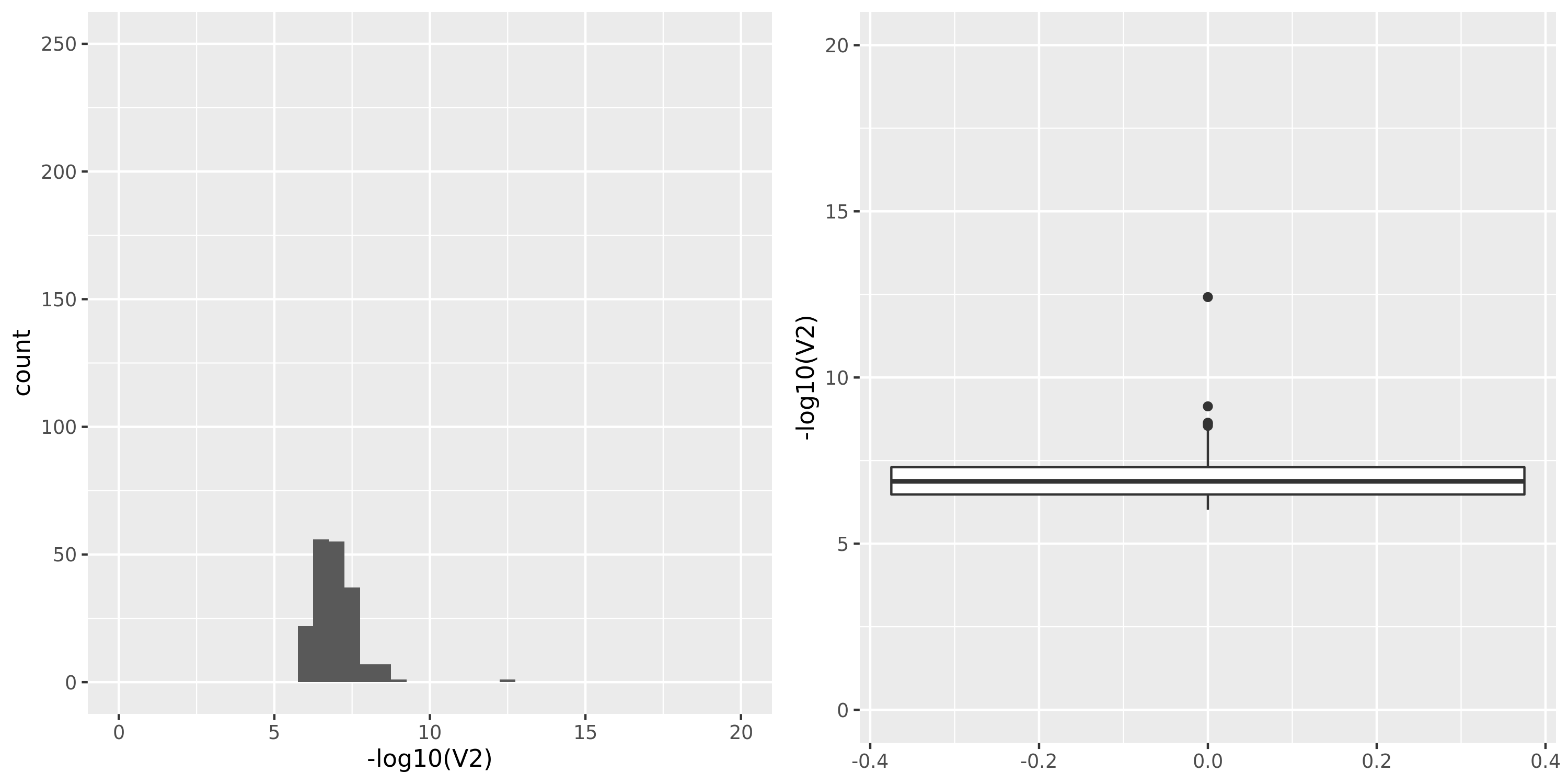
How does zero values affect qvalue?
Short answer:
June 14
Why there are so many eQTLGen signals using PCO_\({\lambda<0.1}\)?
Check the QQ-plot of the observed pvalues from eQTLGen using PCO_\({\lambda<0.1}\) (9918 unique SNPs, all eQTLGen variants) and PCO_\({\lambda<1}\) (909 unique SNPs).
| Version | Author | Date |
|---|---|---|
| 4fc3dff | liliw-w | 2021-06-14 |
June 11
Compare with truncated ‘DGN_transeQTL_battle2014’
In this section, I removed trans-eGenes from Battle’s result that are not included in our analysis for being cross-mappable or poorly mapped. I do this to makes sure univariate and multivariate are based on the same set of genes. I go through the same analysis as below.
- Summary of the new version Battle trans-eQTL signals
After filter our some trans-eGenes, there are 157 (v.s. 736) significant (gene, SNP) pairs left, corresponding to 84 unique trans-eQTLs and 47 unique trans-eGenes.
The following is a a table of the number of trans-target genes of these 84 unique trans-eQTLs.
 1  2  3  4  5 15 16 29
75  1  1  3  1  1  1  1
We have identified 313 unique trans-eQTLs, among which 24 are also detected by Battle’s univariate method. The above table gives which Battle’s signals are replicated by trans-PCO.
Among 84 Battle’s trans-eQTLs, 24 (~28.57%) are also detected by trans-PCO. For 9 signals with more than one trans-target genes included in our analysis, all of them are detected by trans-PCO. Trans-PCO also detected other 15 signals with only one trans-target gene used in our analysis. For the other 60 univariate signals that are missed by trans-PCO, they have only one trans-target gene included in trans-PCO.
            sig N_transeGene if_transPCO num_included
 1:  3:56849749           29        TRUE           29
 2:  3:56858686           16        TRUE           16
 3:  3:56865776           15        TRUE           15
 4:  3:56880444            5        TRUE            5
 5:  3:56871432            4        TRUE            4
 6:  3:56874033            4        TRUE            4
 7:  7:50366637            4        TRUE            4
 8:  3:56851387            3        TRUE            3
 9:  7:50428445            2        TRUE            2
10: 7:106337250            1       FALSE            1
11: 12:54723028            1       FALSE            1
12: 12:54729872            1       FALSE            1
13: 4:103432974            1       FALSE            1
14: 4:103443569            1       FALSE            1
15: 4:103448582            1       FALSE            1
16: 4:103511114            1       FALSE            1
17: 1:118147675            1       FALSE            1
18: 1:118158079            1       FALSE            1
19: 19:37441365            1       FALSE            1
20: 19:37469098            1       FALSE            1
21: 19:37503899            1       FALSE            1
22: 19:37504596            1       FALSE            1
23: 19:37507729            1       FALSE            1
24: 19:37516220            1       FALSE            1
25: 19:37520927            1       FALSE            1
26: 19:37547219            1       FALSE            1
27: 19:37563211            1       FALSE            1
28: 19:37573074            1       FALSE            1
29: 19:37582471            1       FALSE            1
30: 19:37584650            1       FALSE            1
31: 19:37597395            1       FALSE            1
32: 19:37620248            1       FALSE            1
33: 19:37627113            1       FALSE            1
34: 19:37632877            1       FALSE            1
35: 19:37634291            1       FALSE            1
36: 19:37642165            1       FALSE            1
37: 19:37649577            1       FALSE            1
38: 19:37650929            1       FALSE            1
39: 19:37684966            1       FALSE            1
40: 17:33875262            1       FALSE            1
41: 1:248039451            1        TRUE            1
42: 1:248039713            1       FALSE            1
43: 1:248041182            1       FALSE            1
44: 1:248058265            1       FALSE            1
45: 19:44889660            1       FALSE            1
46: 19:44930738            1        TRUE            1
47: 19:44931995            1       FALSE            1
48: 19:44932972            1        TRUE            1
49: 19:44933947            1        TRUE            1
50: 19:44938980            1        TRUE            1
51: 19:44947050            1       FALSE            1
52: 19:44947184            1        TRUE            1
53: 19:44959866            1       FALSE            1
54: 19:44973969            1       FALSE            1
55: 19:44978298            1       FALSE            1
56: 19:44979443            1       FALSE            1
57: 19:44995990            1       FALSE            1
58: 19:45001346            1       FALSE            1
59: 19:45001619            1       FALSE            1
60: 14:35523266            1       FALSE            1
61: 14:35571651            1        TRUE            1
62: 14:35624831            1       FALSE            1
63: 21:44473062            1       FALSE            1
64: 21:44473425            1       FALSE            1
65: 21:44473446            1       FALSE            1
66:  12:8142798            1        TRUE            1
67:  12:8143483            1        TRUE            1
68:  12:8161503            1        TRUE            1
69:  12:8179891            1       FALSE            1
70:  12:8185853            1       FALSE            1
71:  12:8190206            1       FALSE            1
72: 6:159498130            1       FALSE            1
73: 15:80260554            1        TRUE            1
74: 15:80263217            1        TRUE            1
75: 15:80263345            1        TRUE            1
76: 15:80263406            1        TRUE            1
77:  7:50435777            1       FALSE            1
78: 6:169749100            1       FALSE            1
79: 14:20811332            1        TRUE            1
80: 17:33902635            1       FALSE            1
81: 17:34019488            1       FALSE            1
82: 17:34043021            1       FALSE            1
83: 17:34051176            1       FALSE            1
84:  9:99288951            1       FALSE            1
            sig N_transeGene if_transPCO num_included
Compare with ‘DGN_transeQTL_battle2014’
- Summary of Battle trans-eQTL signals
They gave 736 significant (gene, SNP) pairs, corresponding to 350 unique trans-eQTLs and 138 unique trans-eGenes.
The following is a a table of the number of trans-target genes of these 350 unique trans-eQTLs. We can see most of the trans-eQTLs have only 1 or 2 trans-target genes (\(283+34=317, \approx 91\%\)).
  1   2   3   4   5   6   7   8  11  13  14  22  23  24  29  33  59
283  34   3   1  12   1   2   2   2   1   2   1   2   1   1   1   1
Let’s take a look at the trans-eQTLs with more than 2 target genes. We can see these trans-eQTLs are mainly located around the regions 3:56849749, 3:101043565, 7:50366637, 17:33875262.
            sig N_transeGene if_transPCO num_included
 1:  3:56849749           59        TRUE           29
 2:  3:56858686           33        TRUE           16
 3:  3:56865776           29        TRUE           15
 4: 3:101242751           24       FALSE            0
 5: 3:101043565           23       FALSE            0
 6: 3:101106527           23       FALSE            0
 7: 3:101232736           22       FALSE            0
 8: 3:100963761           14       FALSE            0
 9: 3:100970240           14       FALSE            0
10: 3:100994497           13       FALSE            0
11:  3:56851387           11        TRUE            3
12:  3:56880444           11        TRUE            5
13: 3:100915962            8       FALSE            0
14:  7:50366637            8        TRUE            4
15:  3:56874033            7        TRUE            4
16: 3:101068620            7       FALSE            0
17:  3:56871432            6        TRUE            4
18: 3:101042594            5       FALSE            0
19: 3:101080694            5       FALSE            0
20: 3:101085413            5       FALSE            0
21: 3:101135210            5       FALSE            0
22: 3:101160339            5       FALSE            0
23: 3:101184134            5       FALSE            0
24: 3:101191663            5       FALSE            0
25: 3:101231921            5       FALSE            0
26: 3:101237307            5       FALSE            0
27: 3:101252514            5       FALSE            0
28: 3:101253091            5       FALSE            0
29: 3:101253605            5       FALSE            0
30:  7:50428445            4        TRUE            2
31:  7:50435777            3       FALSE            1
32: 17:33875262            3       FALSE            1
33: 17:33902635            3       FALSE            1
sig N_transeGene if_transPCO num_included- As for our results from trans-PCO
We have identified 313 unique trans-eQTLs, among which 24 are also detected by Battle’s univariate method. The above table gives which Battle’s signals are replicated by trans-PCO.
Table of the number of target genes for replicated trans-eQTLs.
 1  2  4  6  7  8 11 29 33 59
12  3  1  1  1  1  2  1  1  1
Signals detected by univariate but missed by trans-PCO.
Since trans-PCO tends to identify SNPs that have effects on multiple genes, I will focus on the univariate trans-eQTLs that correspond to multiple genes (\(>2\)). For this type of signals, there are 33 trans-eQTLs in total, among which 9 are detected by trans-PCO. For the rest of 24 missed trans-eQTLs, there are basically three types: (1) 21 near the region “3:101043565”, (2) 1 at “7:50435777”, (3) 2 at “17:33875262” and “17:33875262”.
Even though the 20 missed trans-eQTLs correspond to multiple genes, ranging from 5 ~ 24, they are still missed by trans-PCO. So I checked their trans-target genes, and it turns out that all of the target genes are filtered out at the beginning of our analysis for being cross-mappable or poorly mapped.
As for the rest of three trans-eQTLs that are missed by trans-PCO, only one of their 3 trans-target genes are included in our analysis.
Take-aways
Trans-PCO tends to be more likely to detect trans-eQTLs with effects on multiple target genes.
Some signals could be missed at the step of filtering out genes.
May 26
Are trans-eQTLs cis-eQTLs?
Updated the way to define cis-eQTLs. Previously, cis-eQTL signals are gene-based (from Pheonix using fastQTL). In this section, I compare trans signals with SNP-based cis-eQTLs from two datasets, i.e. GTEx_v7 (whole blood) and DGN.
GTEx_v7. Here provides all significant variant-gene associations.
DGN. Two steps to obtain SNP-based significant associations.
Gene-based associations. (eGenes using fastQTL, result from Pheonix)
Find all cis-eQTLs for each gene.
See “4.2 cis-eQTL mapping” described here. (p.s. I checked GTEx source code and turns out that the actual code GTEx used is a bit different. See below for key lines.)
pt = mean(c(max(eGene$bpval), min(eGene$bpval)))
eGene$pval_nominal_threshold = signif(qbeta(pt,
eGene$shape1, eGene$shape2, ncp=0, lower.tail=TRUE, log.p=FALSE), 6)| Dataset | #signal | GTEx_v7_is_ciseQTL(SNP-based) | GTEx_v7_cis-eGene | DGN_is_ciseQTL(SNP-based) | DGN_cis-eGene | DGN_is_cissQTL(SNP-based) | DGN_cis-sIntro | DGN_cis-e/sQTL |
|---|---|---|---|---|---|---|---|---|
| DGN | 313 | 51 | 16 | 156 | 39 | 101 | 71 | 182 |
| eQTLGen_DGN | 784 | 221 | 32 | 502 | 83 | 381 | 182 | 551 |
A diagram version:
Are trans-eQTLs cis-e/sQTLs?
| Version | Author | Date |
|---|---|---|
| 1f02e91 | liliw-w | 2021-05-26 |
Observations:
- For DGN, among 313 trans signals, 156 (~49.8%) are also cis-eQTLs, corresponding to 39 eGenes, including:
AC016753.7, BECN1, C17orf50, C2orf68, CFL2, CTD-2562J15.6, ERN1, FAM177A1, FIGNL1, FKRP, GGCX, HABP4, HSD17B1P1, ICAM2, KIAA0391, MAT2A, MLX, NEK6, NFE2, NFKBIA, OR2W3, PARP2, PEX12, PPP2R3C, PRKD2, PSMC3IP, RETSAT, RNF181, RP11-1094M14.8, RP11-69M1.4, RP11-85K15.2, SLC1A5, SLC2A3, SLFN12L, SYMPK, TMEM150A, TTC5, VAMP8, ZNF782
For DGN, 101 (~32.3%) out of 313 trans signals are cis-sQTLs, corresponding to 71 introns. 26 trans-eQTLs are only sQTLs but not eQTLs. These signals are located on chromosome 15 and 19.
Among 313 trans signals, 182 (~58.1%) are either cis-eQTLs or cis-sQTLs.
May 19
How many trans-eQTLs detected in DGN/GTEx whole blood are replicated in eQTLGen?
Replication of DGN signals in eQTLGen. Based on updated results, i.e. smaller and more gene modules & PCO\(_{\lambda>0.1}\).
Are trans-eQTLs cis-eQTLs?
- Dataset: DGN
| Dataset | #signal | is_ciseQTL(gene-based) | is_cissQTL(SNP-based) | is_cise(s)QTL(gene-based) |
|---|---|---|---|---|
| DGN | 313 | 7 | 9 | 15 |
| eQTLGen_DGN | 784 | 17 | 30 | 45 |
Observations:
1.1 DGN
Among 313 trans signals, 7 are also (gene-based) cis-eQTLs, corresponding to 5~7 independent SNPs. The cis-eGenes include SLC2A3, NFE2, KIAA0391, NFKBIA, ERN1, AC016753.7, MAT2A.
Among 313 unique trans signals, 229 (~73%) have a neareset gene that are eGenes (with cis-eQTLs). Among 28 independent trans signals, 19 (~68%) have a neareset gene that are eGenes (with cis-eQTLs).
Among 313 trans signals, 9 are also cis-sQTLs, corresponding to 6 independent SNPs.
1.2 eQTLGen_DGN
Among 784 trans signals, 17 are also (gene-based) cis-eQTLs, corresponding to 9 independent SNPs. The cis-eGenes include AC016753.7, CPEB4, KIAA0391, MAT2A, MRFAP1, NFKBIA, PAQR6, PWP1, RNF181, RP11-539L10.2, RP11-69M1.4, S100P, SENP7, SLC25A44, SLC2A3, SMG5, TMEM79, ZNF782.
Among 784 unique trans signals, 590 (~75%) have a neareset gene that are eGenes (with cis-eQTLs). Among 50 independent trans signals, 29 (~58%) have a neareset gene that are eGenes (with cis-eQTLs).
Among 784 trans signals, 30 are also cis-sQTLs, corresponding to 10 independent SNPs.
Dataset: TCGA
eQTLGen?
March 8
Muscle
Less modules, PCO\(_{\{\lambda: \lambda>0.1\}}\). 1 independent signal, large p.
More modules, PCO\(_{\{\lambda: \lambda>0.1\}}\). 5 independent signal, small p.
More modules, PCO\(_{\{\lambda: \lambda>1\}}\). 5 independent signal, relatively large p.
March 1
Real data analysis by PCO using more \(\lambda\)’s
Dataset: Muscle_Skeletal.
Fewer (independent) signals. \(PCO_{\{\lambda: \lambda>0.1\}}\) (1 signal) v.s. \(PCO_{\{\lambda: \lambda>1\}}\) (3 signals).
proteomics data
See the google doc here.
Other stuff
- RCC account storage
Feb 23
Updated simulation
- Adjusted variance of effects
tests
Oracle: \(\beta^T \Sigma^{-1}Z \approx \beta^T \hat\Sigma^{-1}Z = \beta^T (\sum_{\{\lambda_k: \lambda_k>0.1\}}\lambda_k u_k u_k^T) Z\)
PCO: Use \(\{\lambda_k: \lambda_k>0.1\}\).
scenerios (\(K=100,K=105\))
N: var.b = 0.003; caus = 30%; N.seq = c(200, 400, 600, 800, 1000)
caus: var.b = 0.003; N = 500; caus.seq = c(1, 5, 10, 30, 50, 70, 100)
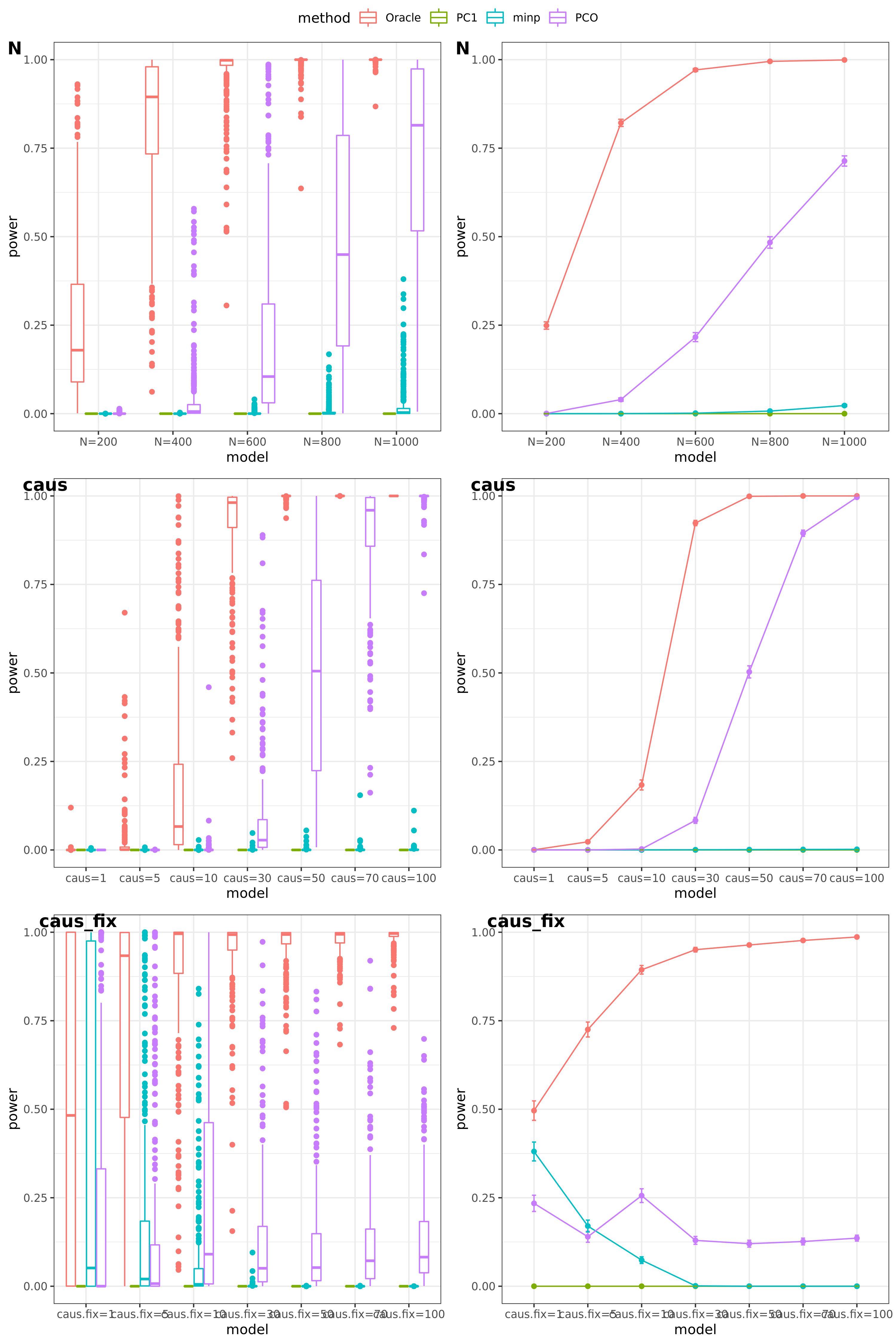
caus_fix: var.b.fix = 0.1; N = 500; caus.seq = c(1, 5, 10, 30, 50, 70, 100)
Run for other \(\Sigma\)’s. \(K=100,K=105\)
FDR level
The minimum null pvalue of PCO is \(\ge 10^{-9}\), similar as the significance threshold we use here \(10^{-9}\).
- Results
power under Bonferroni corretion cutoff
| Version | Author | Date |
|---|---|---|
| cbbe319 | Lili Wang | 2021-02-23 |
Another Sigma (K=105)
| Version | Author | Date |
|---|---|---|
| cbbe319 | Lili Wang | 2021-02-23 |
Feb 16
simulation
tests
Oracle: \(\beta^T \Sigma^{-1}Z \approx \beta^T \hat\Sigma^{-1}Z = \beta^T (\sum_{\{\lambda_k: \lambda_k>1\}}\lambda_k u_k u_k^T) Z\)
PC1;
minp = \(min\{p_1, \dots, p_K \} \times K\)
PCO: Use \(\{\lambda_k: \lambda_k>1\}\).
Multiple testing
The significance threshold is set based on the Bofferroni correction as the \(\frac{0.05}{50\times10^6} = 10^{-9}\) for univariate test and PC-based tests.
scenerios (\(K=100\))
N: var.b = 0.01; caus = 100 (100%); N.seq = c(200, 400, 600, 800, 1000)
caus: var.b = 0.02; N = 500; caus.seq = c(1, 10, 30, 50, 70, 100)
caus_fix: var.b.fix = 0.2; N = 500; caus.seq = c(1, 10, 30, 50, 70, 100)
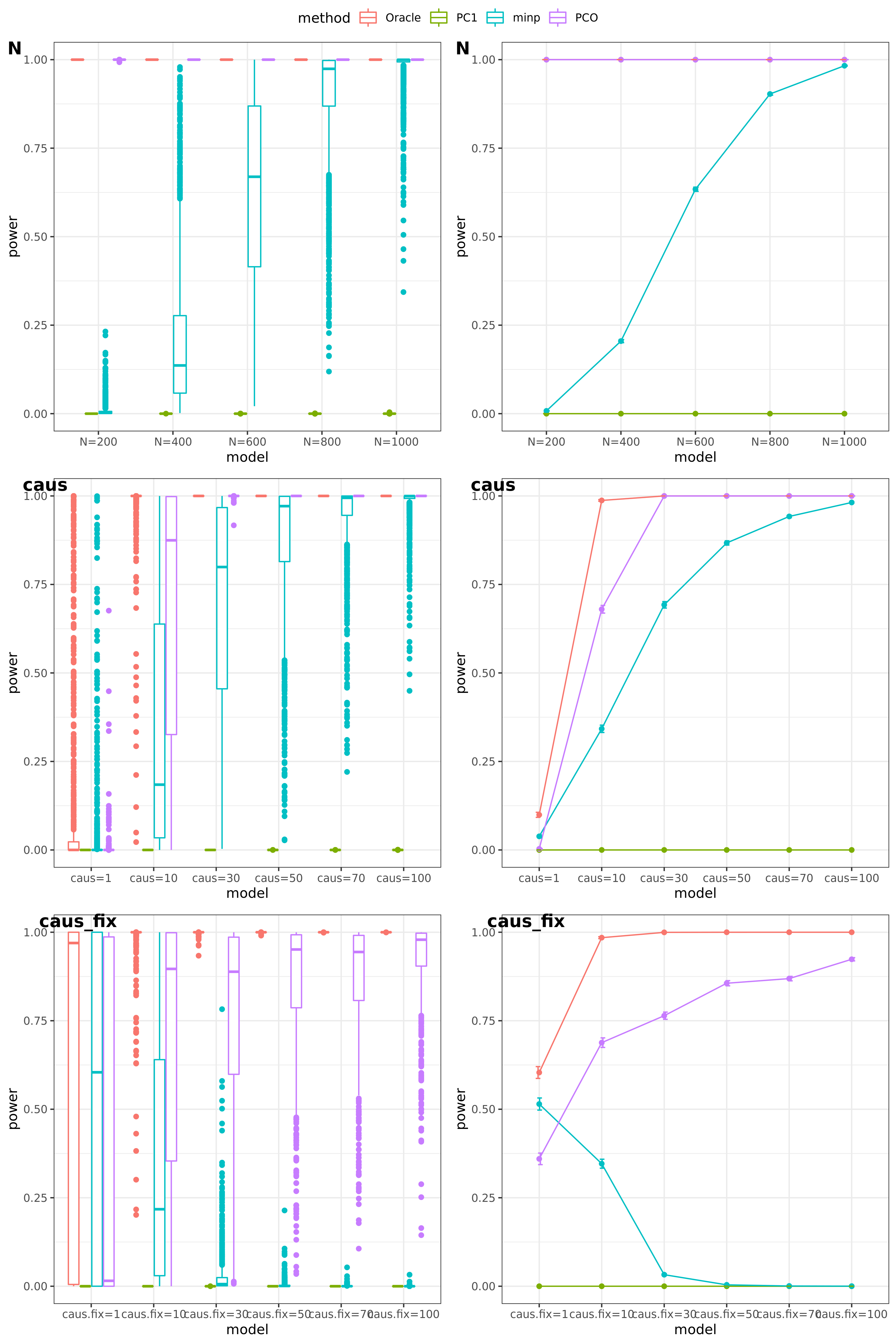
results
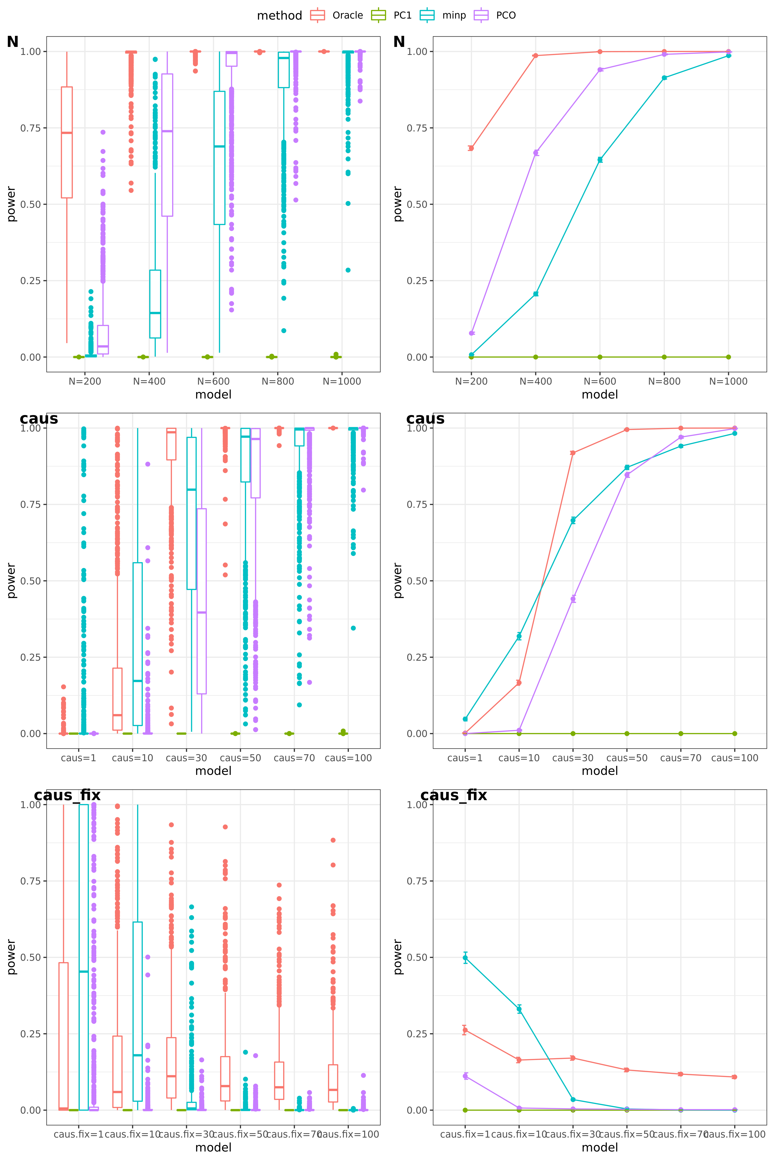
power under Bonferroni corretion cutoff
Try other tests
Oracle: \(\beta^T \Sigma^{-1}Z \approx \beta^T \hat\Sigma^{-1}Z = \beta^T (\sum_{\{\lambda_k: \lambda_k>0.1\}}\lambda_k u_k u_k^T) Z\)
PCO: Use \(\{\lambda_k: \lambda_k>0.1\}\).
power under Bonferroni corretion cutoff
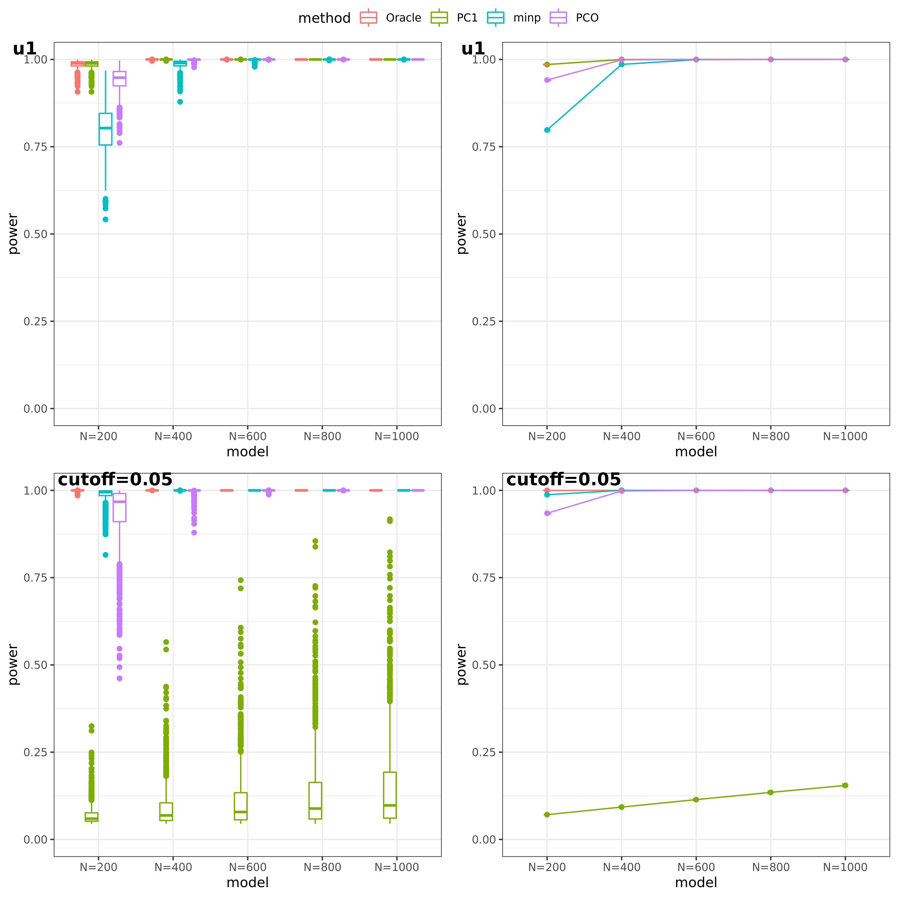
- For talk
(This figure should be updated as for the case of ‘u1’, the threshold is falsely set as 0.05, which should be \(10^{-9}\).)
PC1 v.s. PCO
Jan 26
simulation
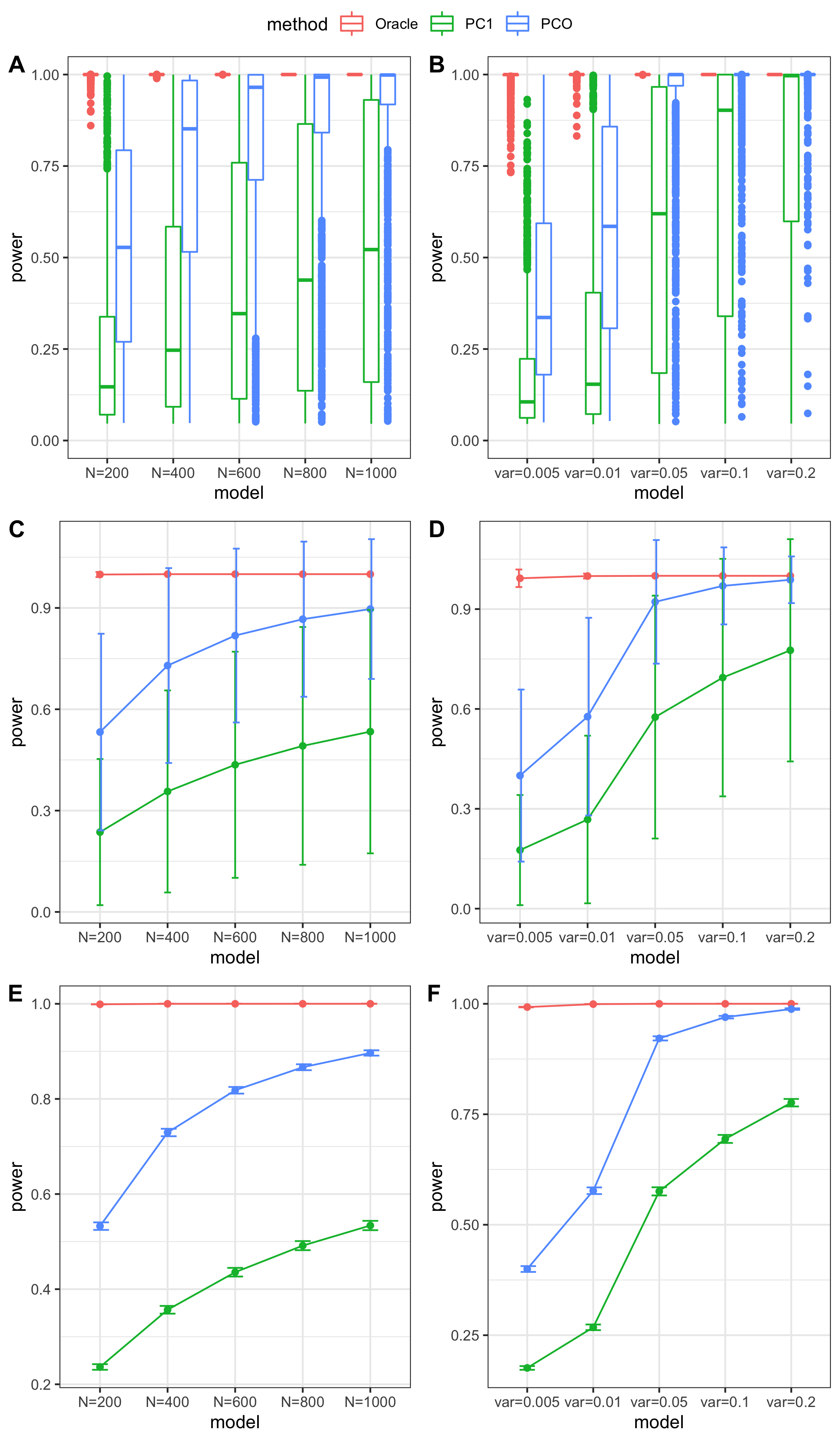
Methods: Oracle, PC1, PCO, MinP, minp.
Models: \(z \sim N(\sqrt{N} \beta, \Sigma)\). \(\beta \sim N(0, \sigma_{b}^2 I_{K \times K})\).
various sample size \(N\). 200, 400, 600, 800, 1000.
various \(\sigma_{b}^2\). 0.005, 0.01, 0.05, 0.1, 0.2.
various causality percentage. ???
simulation.
Generate \(10^4\) zscores under each model. \(10^4\) simulations.
The following plot gives the boxplot, mean plot with standard deviation, and mean plot with standard error of the mean. Which one to use?
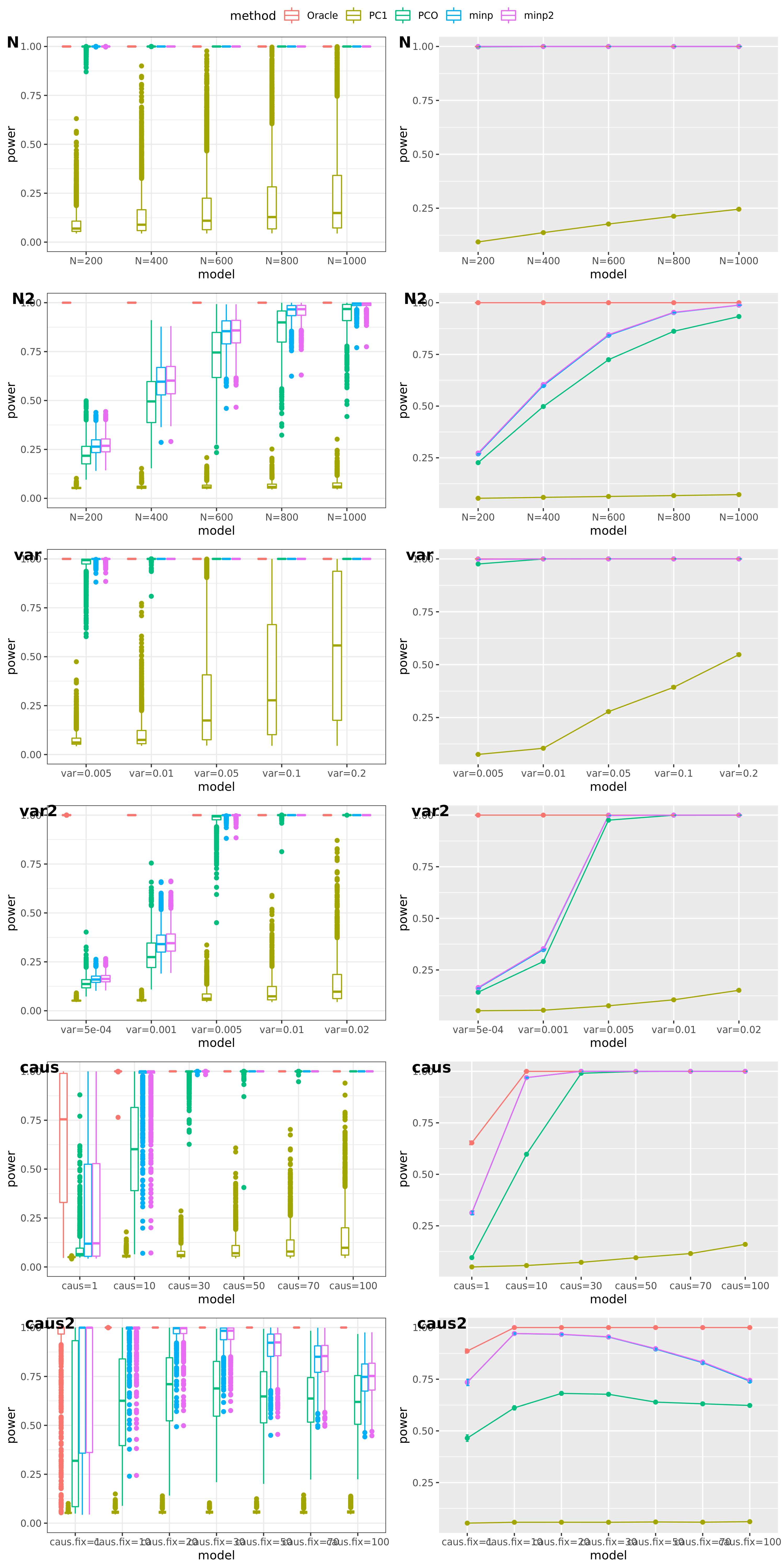
power under cutoff 0.05
| Version | Author | Date |
|---|---|---|
| 8960692 | Lili Wang | 2021-02-16 |
power comparison
| Version | Author | Date |
|---|---|---|
| 8960692 | Lili Wang | 2021-02-16 |
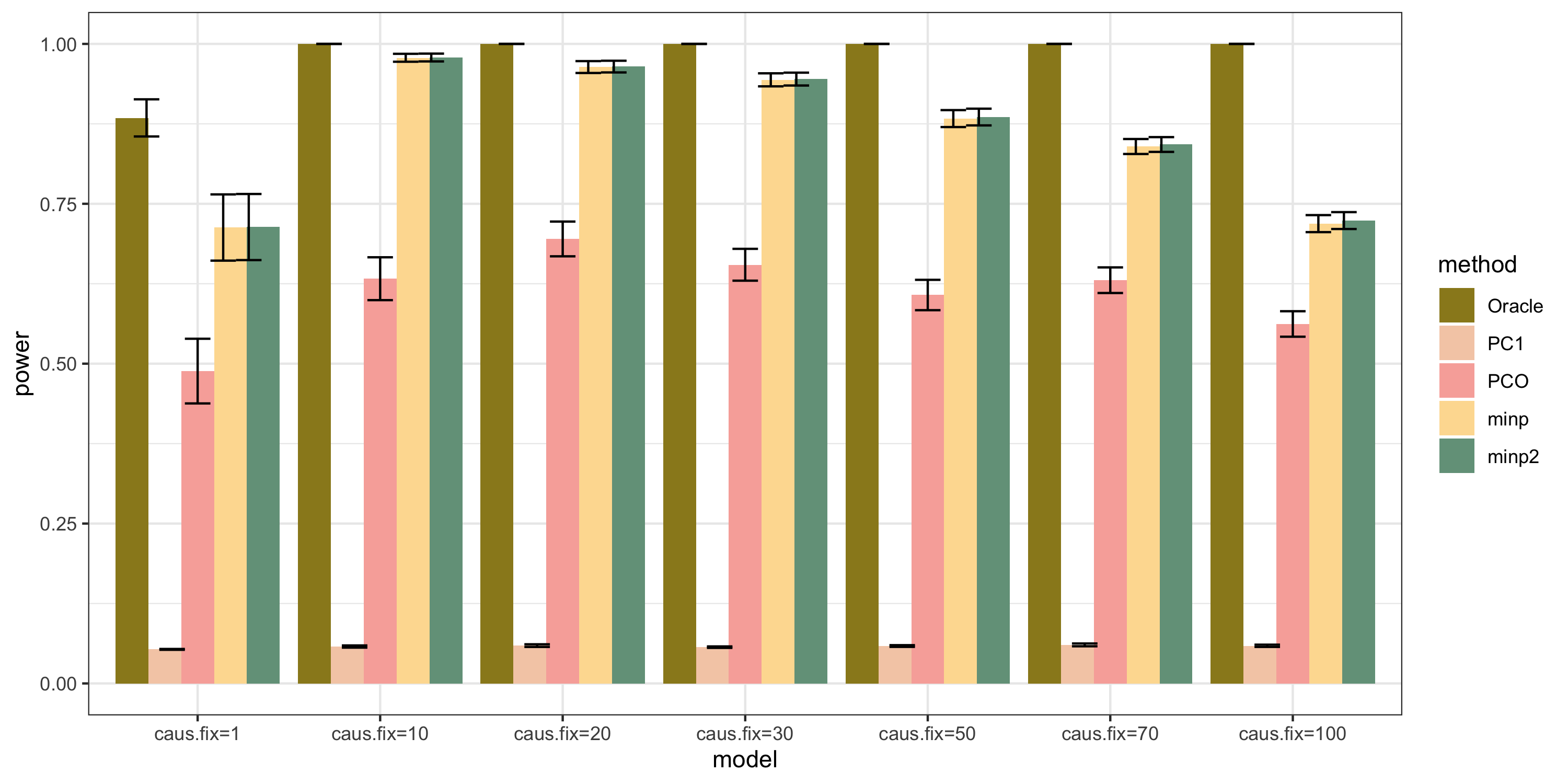
bar plot
| Version | Author | Date |
|---|---|---|
| 912acee | Lili Wang | 2021-02-06 |
Larger FDR level, #signals in large and small module?
Here I will look at how the number of signals changes in the original large and current small modules when I increase the FDR level.
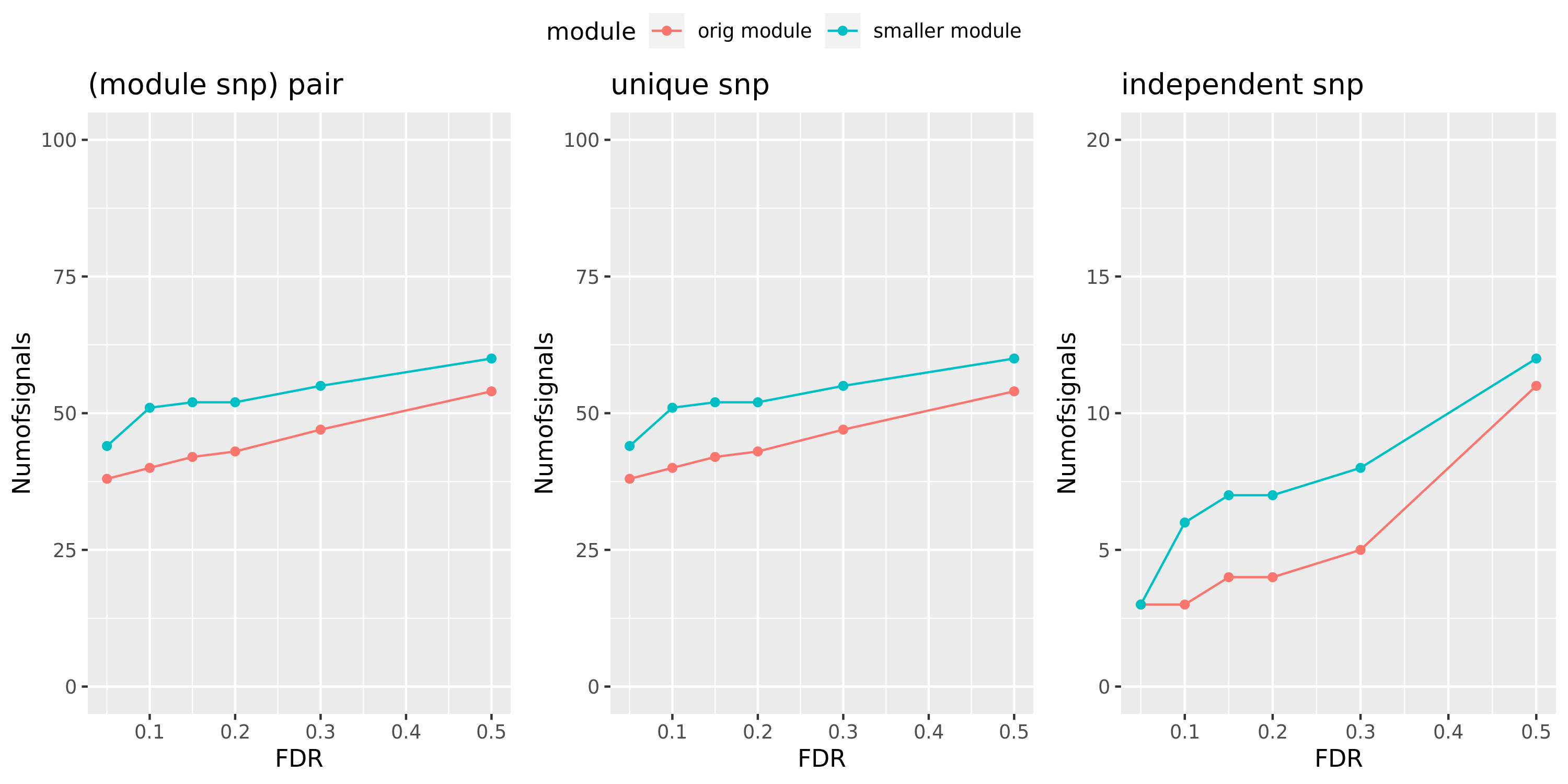
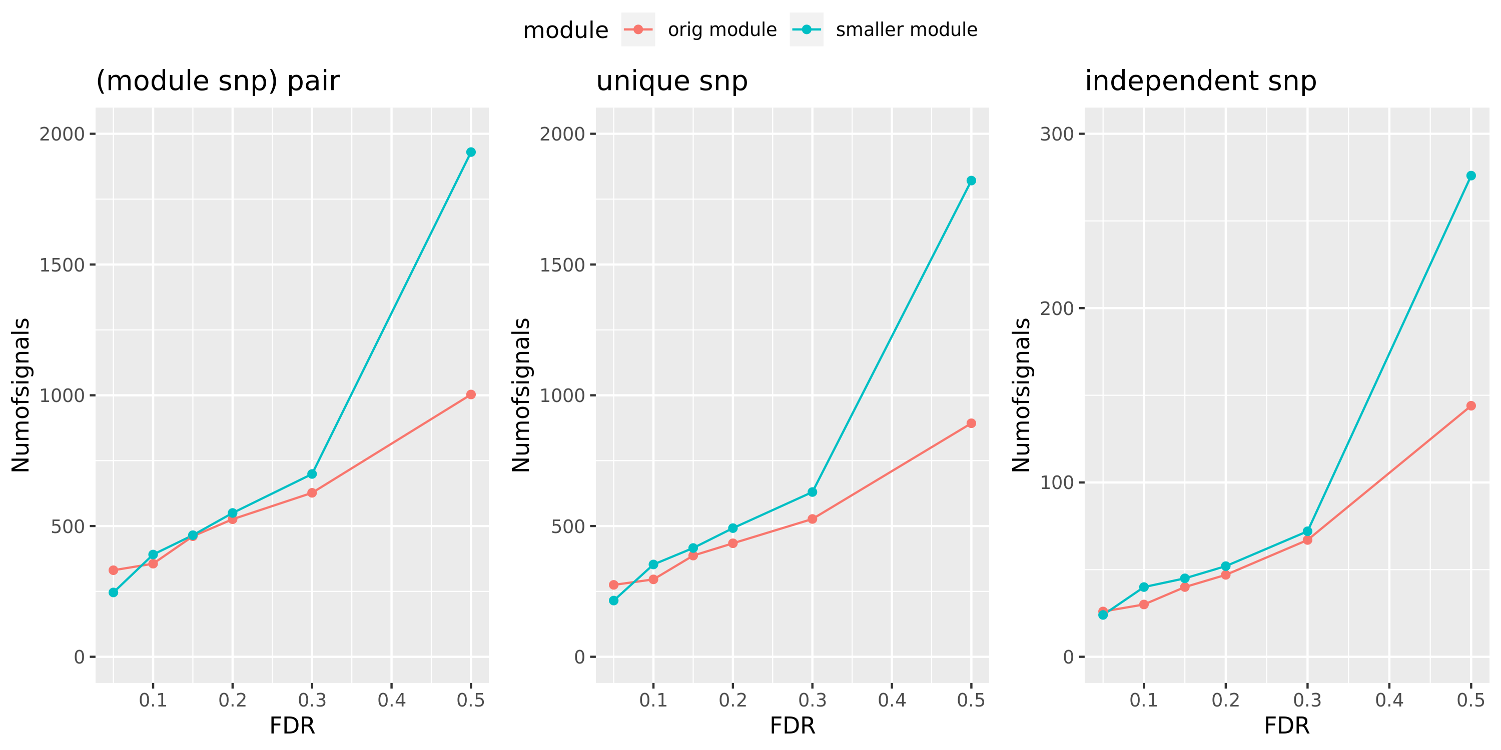
The plot below is based on Muscle tissue from GTEx_v8. The x-axis is for various FDR levels, including 5%, 10%, 15%, and 20%. The y-axis is for the number of signals under these FDR levels. I plot three types of signals, i.e. module and SNP pairs (left subplot), unique SNPs (middle subplot), independent SNPs (right subplot). The two colors represent our previous WGCNA modules (red) and current smaller WGCNA modules (blue).
We can observe (1) When increasing FDR levels, number of signals only increase a little bit, say 3-5 more signals. This means that the corrected pvalues are bipolar, i.e. either very small or very large. (2) Signals based on smaller modules are similar to that of previous standard modules.
Muscle: #signals v.s.FDR
| Version | Author | Date |
|---|---|---|
| 0b5d8d3 | Lili Wang | 2021-02-02 |
DGN: #signals v.s.FDR
| Version | Author | Date |
|---|---|---|
| 0b5d8d3 | Lili Wang | 2021-02-02 |
Smaller gene modules, more signals?
I changed the parameter deepSplit in function cutreeDynamic from package WGCNA to get modules with smaller size. I run it on the Muscle tissue from GTEx (see GTEx_v8.Muscle_Skeletal.WGCNA in the GTEx results table). Compared to GTEx_v8.Muscle_Skeletal, though more modules (32 v.s. 18), they have same independent signals (3), located on chr5, chr10, and chr22.
The corresponding modules of these signals from small and large WGCNA share a large proportion of genes.
| signal.Chr | module.small (#genes) | module.big (#genes) | #overlapped genes |
|---|---|---|---|
| chr5 | module21 (89) | module15 (114) | 88 |
| chr10 | module21 (89) | module15 (114) | 88 |
| chr22 | module2 (297) | module4 (350) | 257 |
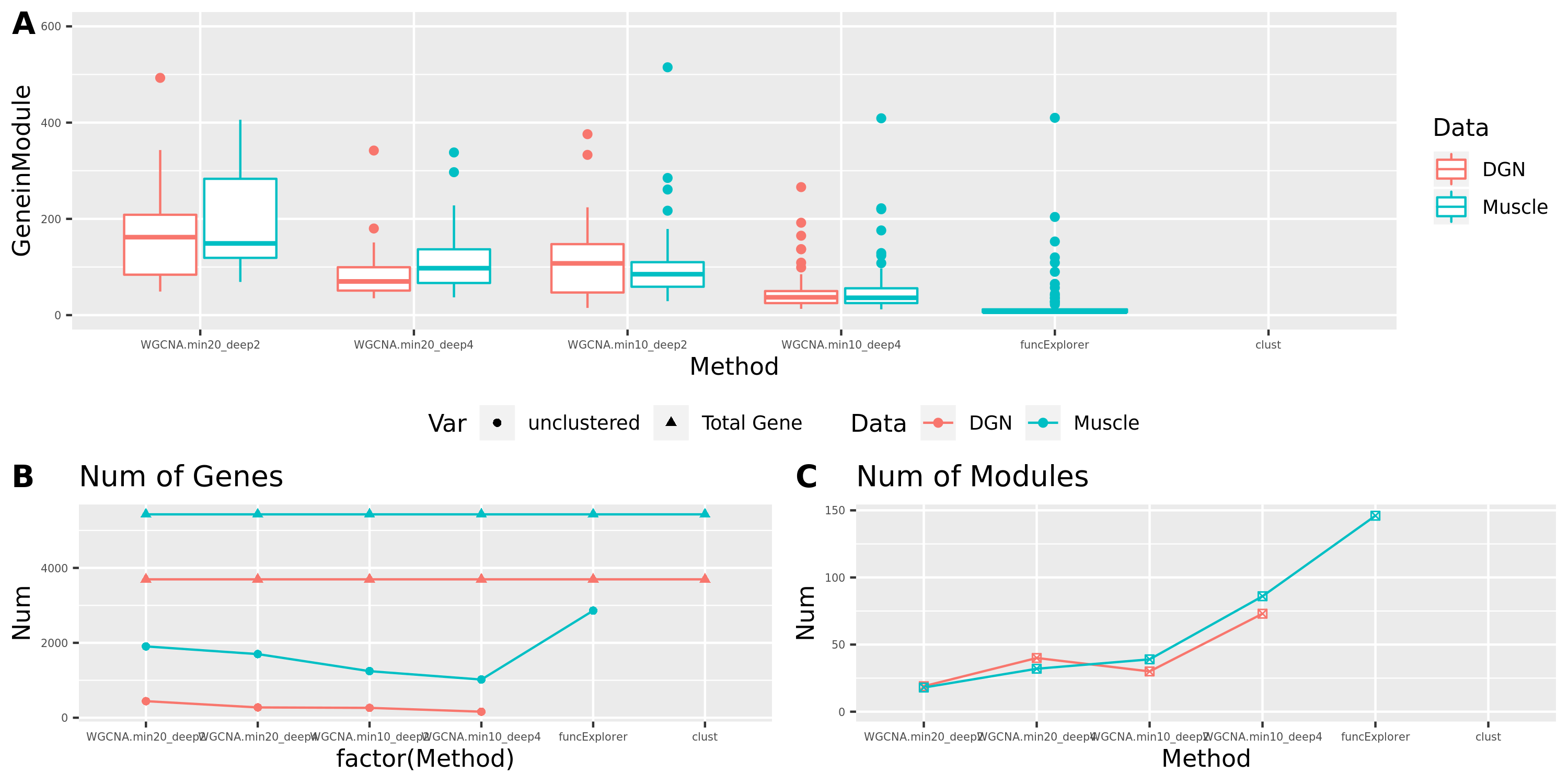
The above table is for clusters obtained by method ‘WGCNA.min20_deep2’ (big) and ‘WGCNA.min20_deep4’ (small). Next, I give more info about the clusters by more methods, i.e. #genes in modules (A), #unclassfied genes (B), and #modules (C) by the six methods. I also give the pvalue distribution corresponding to these clusters below.
Generally, funcExplorer gives more modules, smaller module, and much more unclassified genes. Though the smaller modules, there aren’t many extreme pvalues. Say, the minimum p of all is about \(10^{-9}\), as compared to \(10^{-14}\) by other methods.
From the pvalue plot, it looks like ‘WGCNA.min10_deep4’ gives smaller clusters and some extreme pvalues. So next step I will run the whole pipleline for this setting.
Modules v.s. methods/parameters
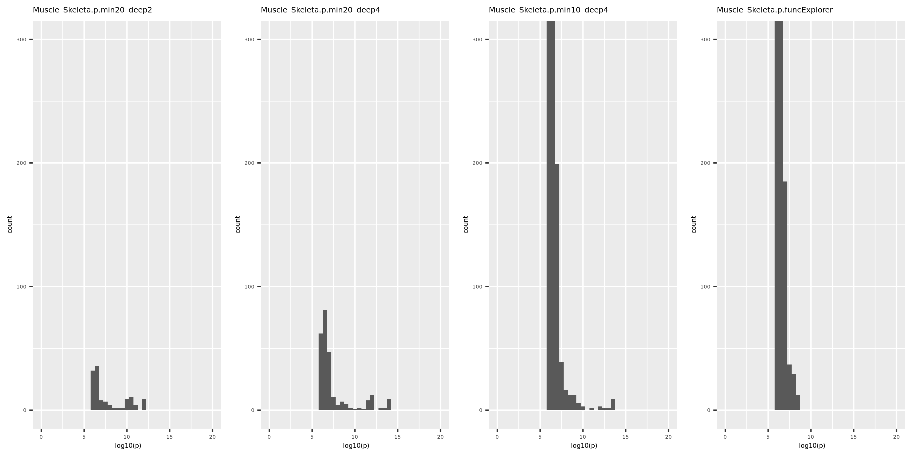
p distribution of Muscle
| Version | Author | Date |
|---|---|---|
| 74c629e | Lili Wang | 2021-02-06 |
Jan 05, Jan 19
Simulation
The simulations here aim to compare the power of PC-based tests including PC1 (using only the primary PC) and PCO (using combined PC’s), and non-PC based test MinP. The simulations consist of two parts: (1) verify that type 1 error is well controlled; (2) compare power of tests. At this time, I simply assume there is no LD among SNPs, i.e. tests are independent.
- Verify that type 1 error is well controlled.
Since the tests are assumed to be independent, the null pvalues should be uniformly distributed. To verify that, I estimate the null pvalues by empirical p’s obtained from the following steps.
Step1. Generate \(z_0 \sim N(0, \Sigma) | H_0\).
Step2. Run tests including PC1, PCO, MinP for \(10^6\) times and obtain \(10^6\) p’s for each test.
Step3. Compute the empirical T1E at significance \(\alpha\) by \(\frac{I\{p<\alpha\}}{10^6}\). Draw qqplot of \(-log_{10}p\).
The correlation matrix \(\Sigma\) is the correlation of genes in module15 of GTEx dataset Muscle_Skeletal (Sigma.Muscle_Skeletal.module15.chr7.rds).
| alpha | PC1 | PCO | MinP |
|---|---|---|---|
| 5e-02 | 0.050356 | 0.053584 | |
| 1e-04 | 0.000093 | 0.000114 |
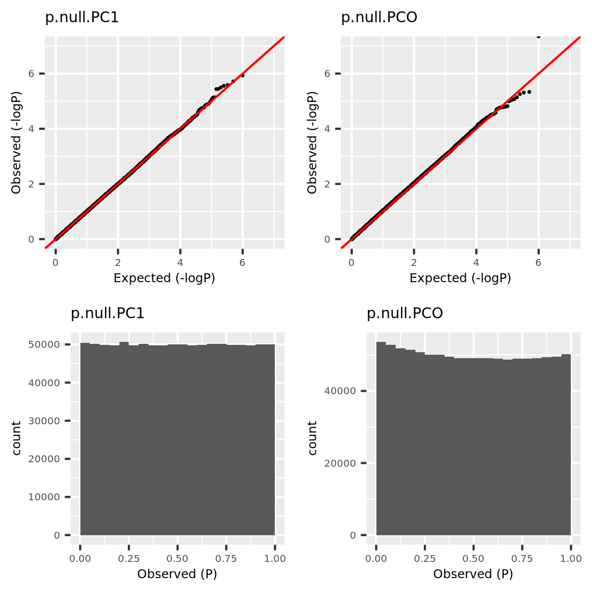
qqplot.simulation.null
| Version | Author | Date |
|---|---|---|
| 11c79eb | Lili Wang | 2021-01-19 |
- Compare power of tests.
To compare the power of non-/PC-based tests, I will run the oracle test in addition to PC1, PCO, and MinP to benchmark the power. It’s mentioned in the PCO paper that given a fixed correlation relationship among the phenotypes, the power of a test depends on the relationship bewteen the true effects (\(\beta\)) and the phenotype correlation (\(\Sigma\)). Therefore, to see which tests perform well in what cases, I will consider different models, including (1) \(\beta=10 u_1\); (2) \(\beta=4 u_k\); (3) \(\beta=1.5 u_K\); (4) \(\beta=rnorm(K)\); (5) \(\beta=rnorm(0.7K)\); (6) \(\beta=rnorm(0.3K)\).
Step1. Generate \(z_0 \sim N(\beta, \Sigma) | H_1\).
Step2. Run tests including Oracle, PC1, PCO, MinP for \(10^6\) times and obtain \(10^6\) p’s for each test.
Step3. Compute the power at significance \(\alpha\) by \(\frac{I\{p<\alpha\}}{10^6}\).
| Model | Oracle | PC1 | PCO | MinP |
|---|---|---|---|---|
| u1 | 0.946341 | 0.902540 | 0.746301 | |
| uPCO | 0.989835 | 0.050178 | 0.713434 | |
| uK | 0.953727 | 0.049719 | 0.054140 | |
| 100% | 1.000000 | 0.058867 | 0.945918 | |
| 70% | 1.000000 | 0.058910 | 0.580368 | |
| 30% | 0.999995 | 0.050201 | 0.149904 |
GTEx
Results
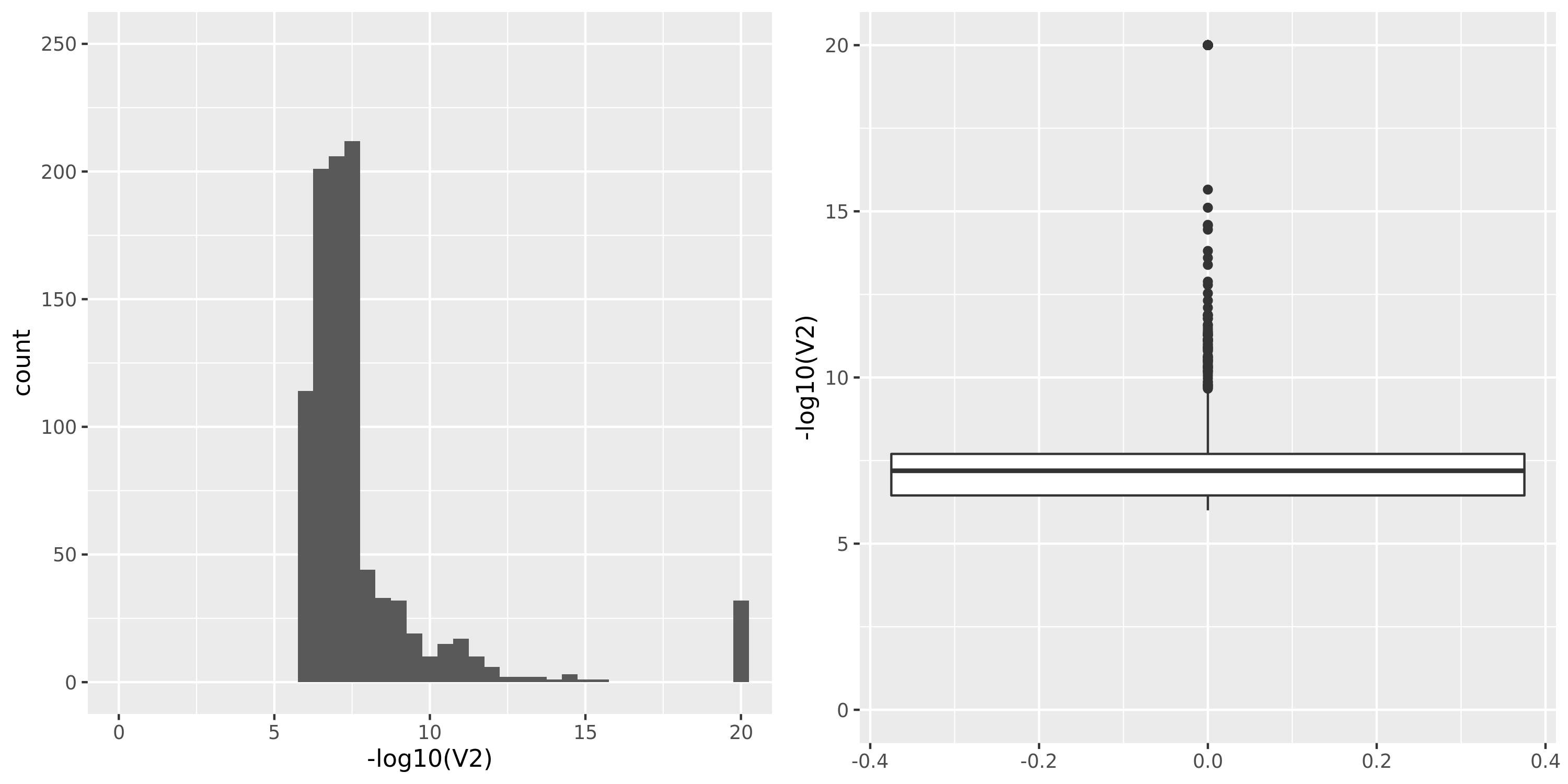
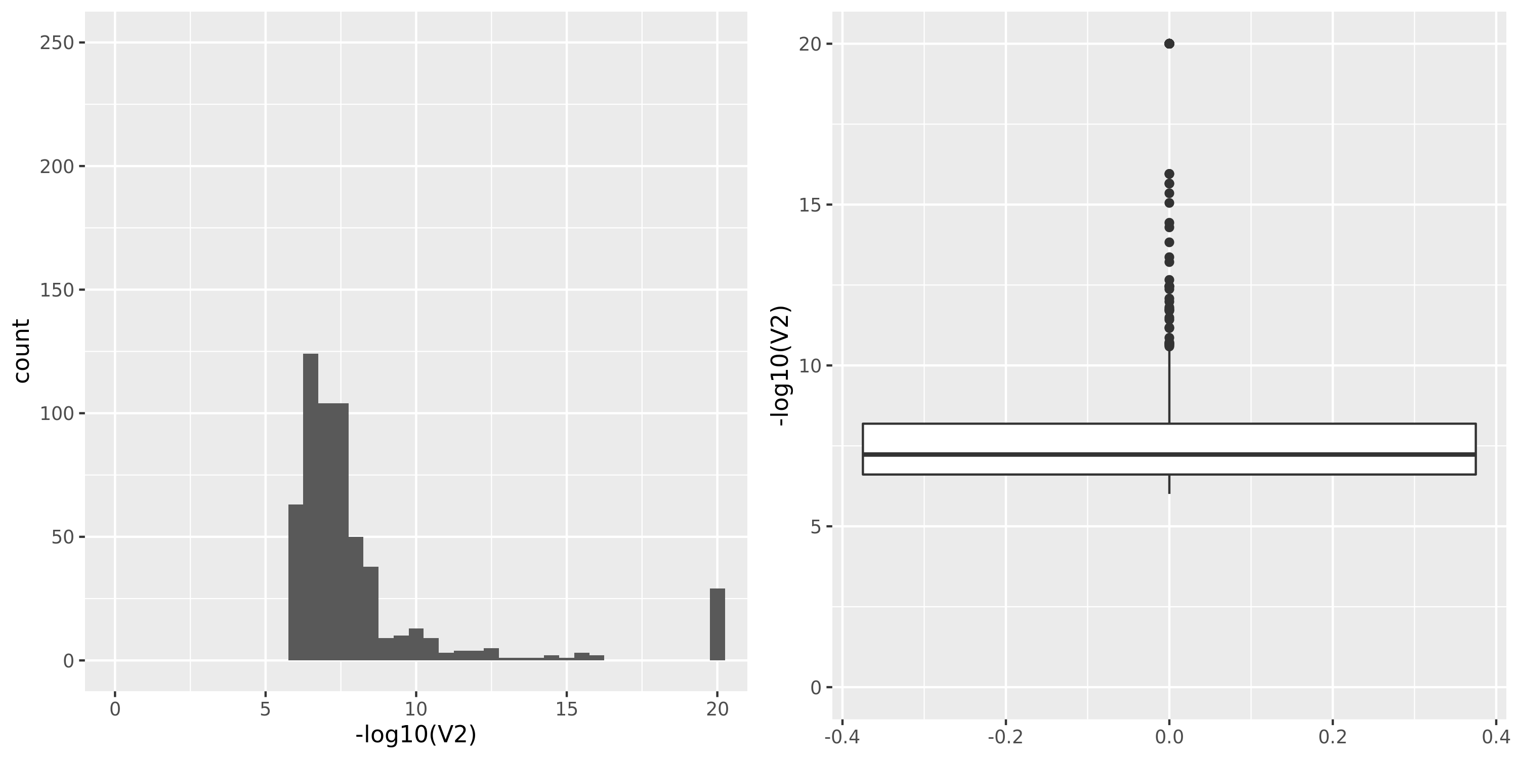
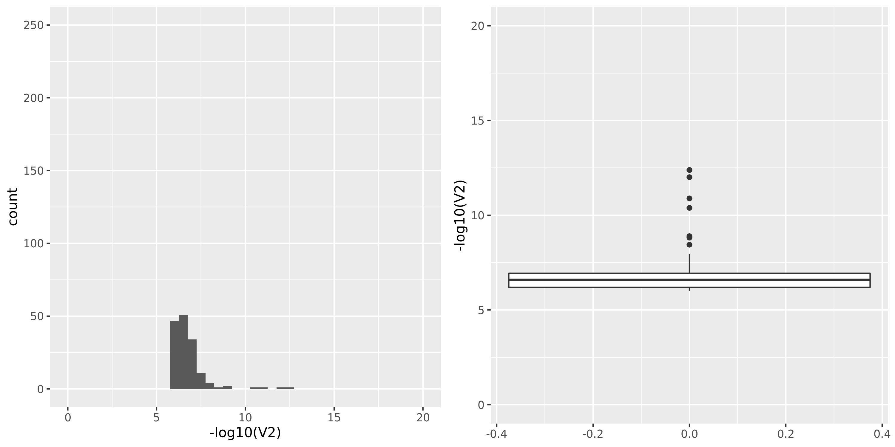
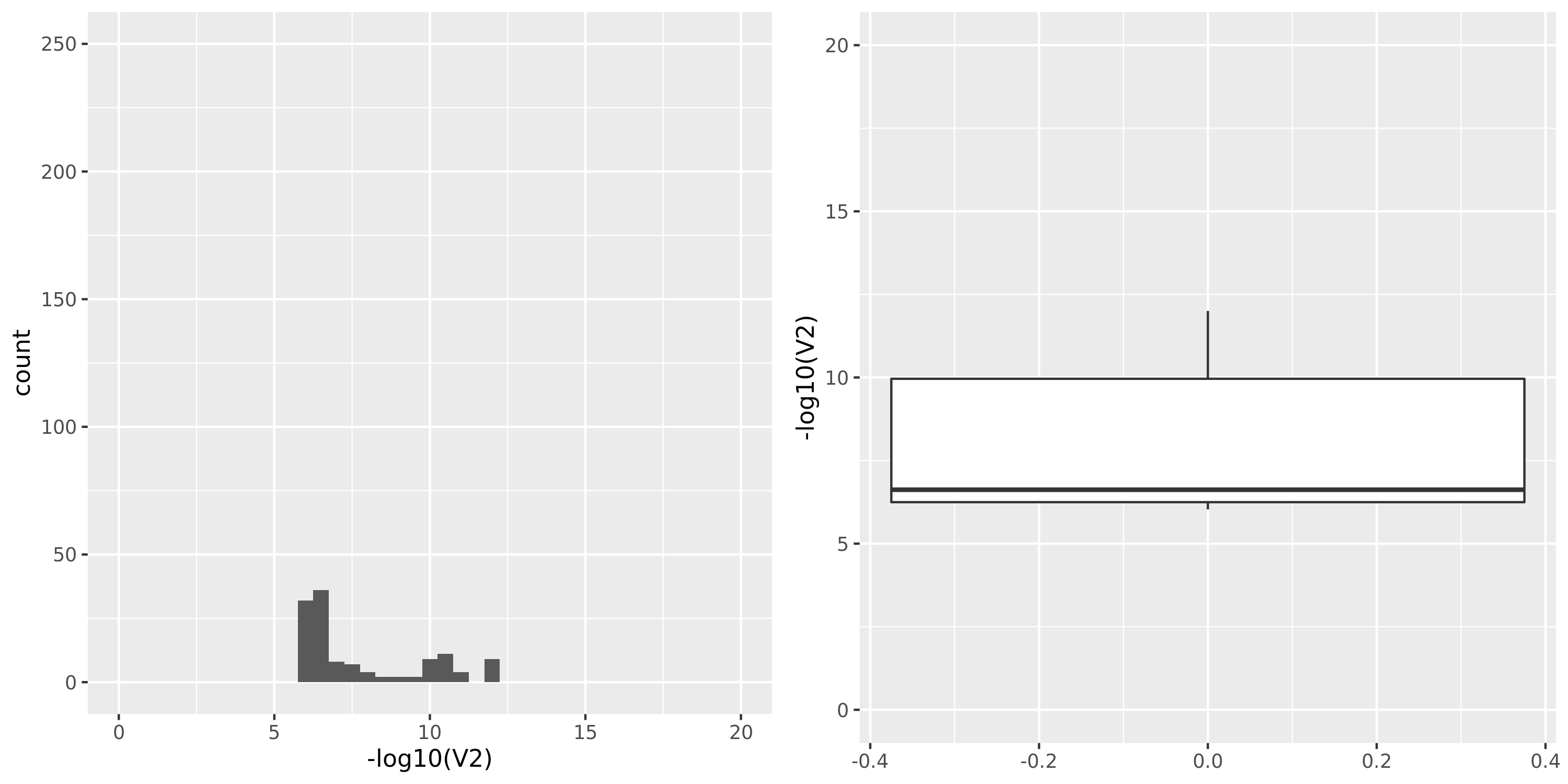
The table below summarizes all results I have so far, followed by figures of the distributions of pvalues in various datasets.
| Dataset | Nsample | All | Annotated | Filtered | Filtered_info | Final | Nmodule | FDR | Nperm | QTL_Module | unique_QTL | independent_QTL |
|---|---|---|---|---|---|---|---|---|---|---|---|---|
| DGN | 913 | 13634 | 11979 | 8120 | 0;165;1663;8073 | 3859 | 21 | combined chr+module | 20 | 659 | 623 | 40 |
| DGN_new | 913 | 13634 | 12585 | 9939 | 1;453;1798;8705 | 3695 | 19 | combined chr+module | 10 | 331 | 275 | 26 |
| TCGA | 788 | 17656 | 15994 | 12694 | 336;3504;10697;598 | 4962 | ||||||
| GTEx_v8.Whole_Blood | 670 | 20315 | 20315 | 15245 | 619;4544;3677;13096 | 5070 | 22 | combined chr+module | 10 | 4 | 4 | 2 |
| GTEx_v8.Muscle_Skeletal | 706 | 21031 | 21031 | 15601 | 675;4447;3631;13490 | 5430 | 18 | combined chr+module | 10 | 38 | 38 | 3 |
| GTEx_v8.Skin_Sun_Exposed_Lower_leg | 605 | 25196 | 25196 | 18801 | 807;6458;4557;15650 | 6395 | 30 | combined chr+module | 10 | 1 | 1 | 1 |
| GTEx_v8.Artery_Tibial | 584 | 23304 | 23304 | 17390 | 795;5588;4202;14730 | 5914 | 20 | combined chr+module | 10 | 0 | 0 | 0 |
| GTEx_v8.Muscle_Skeletal.cross | 706 | 21031 | 21031 | 7141 | 675;4447;3631;0 | 13890 | 39 | combined chr+module | 10 | 43 | 43 | 4 |
| GTEx_v8.Muscle_Skeletal.WGCNA | 706 | 21031 | 21031 | 15601 | 675;4447;3631;13490 | 5430 | 32 | combined chr+module | 10 | 44 | 44 | 3 |
| DGN_new.WGCNA | 913 | 13634 | 12585 | 9939 | 1;453;1798;8705 | 3695 | 40 | combined chr+module | 10 | |||
| TCGA_new |
DGN
| Version | Author | Date |
|---|---|---|
| b110975 | Lili Wang | 2020-12-17 |
DGN_new
| Version | Author | Date |
|---|---|---|
| 361c43e | Lili Wang | 2021-01-04 |
Whole_Blood
| Version | Author | Date |
|---|---|---|
| 361c43e | Lili Wang | 2021-01-04 |
Muscle_Skeletal
| Version | Author | Date |
|---|---|---|
| 361c43e | Lili Wang | 2021-01-04 |
Skin_Sun_Exposed_Lower_leg
| Version | Author | Date |
|---|---|---|
| 361c43e | Lili Wang | 2021-01-04 |
Artery_Tibial
| Version | Author | Date |
|---|---|---|
| 361c43e | Lili Wang | 2021-01-04 |
Muscle_Skeletal.cross
| Version | Author | Date |
|---|---|---|
| 60cf10e | Lili Wang | 2021-01-17 |
Remarks
The dataset “DGN_new” represents DGN through the standard filtering (see “Gene filter” on Dec 10).
GTEx datasets generally have few significant signals and relatively large pvalues (compared to DGN).
The dataset “GTEx_v8.Muscle_Skeletal.cross” uses Muscle_Skeletal samples from GTEx_v8 (similar as GTEx_v8.Muscle_Skeletal), but without removing cross-mapped genes before constructing gene modules. Therefore, there are 13890 genes (v.s. 5430 in GTEx_v8.Muscle_Skeletal) in total which result in 39 modules (v.s. 18 in GTEx_v8.Muscle_Skeletal). We do this step because we observed that there are relatively few signals using our original pipeline and we wonder if the reason to this observation is us filtering too many genes in the first step and leaving too few signals. To check on this, we put the “filtering” to the last step, i.e. including potentially cross-mapped genes into the analysis and generate significant variant-module pairs. We then exclude those where target eGene in the module is cross-mappable with any gene within 1Mb of the variant. Hopefully we could have more signals.
However, though the increased genes and modules, the number of identified signals (43) is similar as that using the original pipeline (38). Next, I will look into these signals.
| variant-module | p | q |
|---|---|---|
| module15:10:48930105 | 8.63e-10 | 8.33e-03 |
| module15:5:132440814 | 1.56e-09 | 2.16e-02 |
| module15:5:132448891 | 3.36e-09 | 4.74e-02 |
| module15:5:132450078 | 5.81e-12 | 0.00e+00 |
| module15:5:132450726 | 5.96e-12 | 0.00e+00 |
| module15:5:132450916 | 8.89e-12 | 0.00e+00 |
| module15:5:132451361 | 5.97e-11 | 0.00e+00 |
| module15:5:132451586 | 1.11e-11 | 0.00e+00 |
| module15:5:132453865 | 1.05e-12 | 0.00e+00 |
| module15:5:132454053 | 9.94e-13 | 0.00e+00 |
| module15:5:132454171 | 1.03e-12 | 0.00e+00 |
| module15:5:132454631 | 1.44e-12 | 0.00e+00 |
| module15:5:132454724 | 1.08e-12 | 0.00e+00 |
| module15:5:132455672 | 1.07e-12 | 0.00e+00 |
| module15:5:132455979 | 1.04e-12 | 0.00e+00 |
| module15:5:132456154 | 9.96e-13 | 0.00e+00 |
| module15:5:132456710 | 6.04e-11 | 0.00e+00 |
| module15:5:132458606 | 5.33e-11 | 0.00e+00 |
| module15:5:132459905 | 4.84e-11 | 0.00e+00 |
| module15:5:132459971 | 5.04e-11 | 0.00e+00 |
| module15:5:132460190 | 5.05e-11 | 0.00e+00 |
| module15:5:132460375 | 5.56e-11 | 0.00e+00 |
| module15:5:132460917 | 5.03e-11 | 0.00e+00 |
| module15:5:132461111 | 5.17e-11 | 0.00e+00 |
| module15:5:132463834 | 5.47e-11 | 0.00e+00 |
| module15:5:132464413 | 3.90e-11 | 0.00e+00 |
| module15:5:132464907 | 1.01e-12 | 0.00e+00 |
| module15:5:132466034 | 4.56e-11 | 0.00e+00 |
| module15:5:132468333 | 1.32e-10 | 0.00e+00 |
| module15:5:132468353 | 5.74e-11 | 0.00e+00 |
| module15:5:132468564 | 8.53e-11 | 0.00e+00 |
| module15:5:132469724 | 5.63e-11 | 0.00e+00 |
| module15:5:132469899 | 6.96e-11 | 0.00e+00 |
| module15:5:132470043 | 1.03e-10 | 0.00e+00 |
| module15:5:132470796 | 5.42e-11 | 0.00e+00 |
| module15:5:132471932 | 8.01e-11 | 0.00e+00 |
| module15:5:132474927 | 2.71e-10 | 2.94e-03 |
| module4:22:23508295 | 3.76e-10 | 5.71e-03 |
| variant-module | p | q |
|---|---|---|
| module8:1:123955560 | 9.97e-12 | 0.00e+00 |
| module8:1:123955561 | 1.06e-11 | 0.00e+00 |
| module8:16:36353041 | 3.49e-11 | 6.67e-03 |
| module8:16:36353056 | 8.29e-11 | 1.25e-02 |
| module8:5:132453865 | 1.56e-09 | 3.12e-02 |
| module8:5:132454053 | 1.59e-09 | 2.86e-02 |
| module8:5:132454171 | 1.52e-09 | 3.33e-02 |
| module8:5:132454631 | 1.43e-09 | 3.57e-02 |
| module8:5:132454724 | 1.53e-09 | 3.23e-02 |
| module8:5:132455672 | 1.50e-09 | 3.45e-02 |
| module8:5:132455979 | 1.56e-09 | 3.03e-02 |
| module8:5:132456154 | 1.78e-09 | 3.42e-02 |
| module8:5:132456710 | 1.36e-09 | 3.33e-02 |
| module8:5:132458606 | 3.37e-10 | 1.76e-02 |
| module8:5:132459905 | 6.50e-10 | 1.74e-02 |
| module8:5:132459971 | 3.92e-10 | 1.43e-02 |
| module8:5:132460190 | 3.50e-10 | 1.58e-02 |
| module8:5:132460375 | 3.37e-10 | 1.67e-02 |
| module8:5:132460917 | 3.98e-10 | 1.36e-02 |
| module8:5:132461111 | 3.57e-10 | 1.50e-02 |
| module8:5:132463834 | 8.21e-10 | 2.40e-02 |
| module8:5:132464413 | 9.93e-10 | 2.69e-02 |
| module8:5:132466034 | 6.75e-10 | 1.67e-02 |
| module8:5:132468333 | 1.86e-09 | 3.50e-02 |
| module8:5:132468353 | 1.69e-09 | 3.06e-02 |
| module8:5:132468564 | 2.43e-09 | 4.19e-02 |
| module8:5:132469724 | 1.93e-09 | 3.66e-02 |
| module8:5:132469899 | 1.73e-09 | 3.24e-02 |
| module8:5:132470043 | 1.56e-09 | 2.94e-02 |
| module8:5:132470796 | 1.85e-09 | 3.33e-02 |
| module8:5:132471932 | 2.37e-09 | 4.29e-02 |
| module8:5:46659000 | 9.86e-13 | 0.00e+00 |
| module8:5:46906585 | 2.34e-11 | 7.14e-03 |
| module8:5:47027928 | 0.00e+00 | 0.00e+00 |
| module8:5:47068540 | 0.00e+00 | 0.00e+00 |
| module8:5:47166316 | 3.33e-16 | 0.00e+00 |
| module8:5:47210790 | 0.00e+00 | 0.00e+00 |
| module8:5:47210990 | 0.00e+00 | 0.00e+00 |
| module8:5:47258679 | 4.44e-16 | 0.00e+00 |
| module8:5:47258917 | 3.33e-16 | 0.00e+00 |
| module8:5:49809727 | 2.70e-13 | 0.00e+00 |
| module8:5:49930686 | 0.00e+00 | 0.00e+00 |
| module8:5:49936394 | 1.10e-11 | 0.00e+00 |
For GTEx_v8.Muscle_Skeletal, there are 38 variant-module pairs, corresponding to 2 module (module 15, module4) and 3 independent loci on (chr5, chr10, chr22). GTEx_v8.Muscle_Skeletal.cross has 43 variant-module pairs, corresponding to 1 module (module 8) and 4 independent loci on (chr1, chr5, chr16).
The signal on chr5 is significant for both module 15 (114 genes) and module 8 (394 genes) in two datasets, which have 82 shared genes. Take SNP [rs2706381][rs2706381 GTEx ref] (chr5:132474927) for example. It is ["in cis with IRF1 ($P \le 2\times10^{-10}$; Fig. 6c), a transcription factor that facilitates regulation of the interferon-induced immune response"][rs2706381 GTEx ref]. It is also ["associated in trans with PSME1 ($P \le 1.1\times10^{-11}$) and PARP10 ($P \le 7.8\times10^{-10}$)"][rs2706381 GTEx ref]. These two genes are included in module 15. The reference also gives additional results to "suggest that cis-regulatory loci affecting IRF1 are regulators of interferon-responsive inflammatory processes involving genes including PSME1 and PARP10, with implications for complex traits specific to muscle tissue".
I also looked at the enrichment of the genes in module 15. These genes are mainly enriched in immunity-related terms and tuberculosis. To reproduce, use the gene list [here](./gene.GTEx_v8.Muscle_Skeletal.module15.txt).
SNP 10:48930105. module 15.
module4:22:23508295
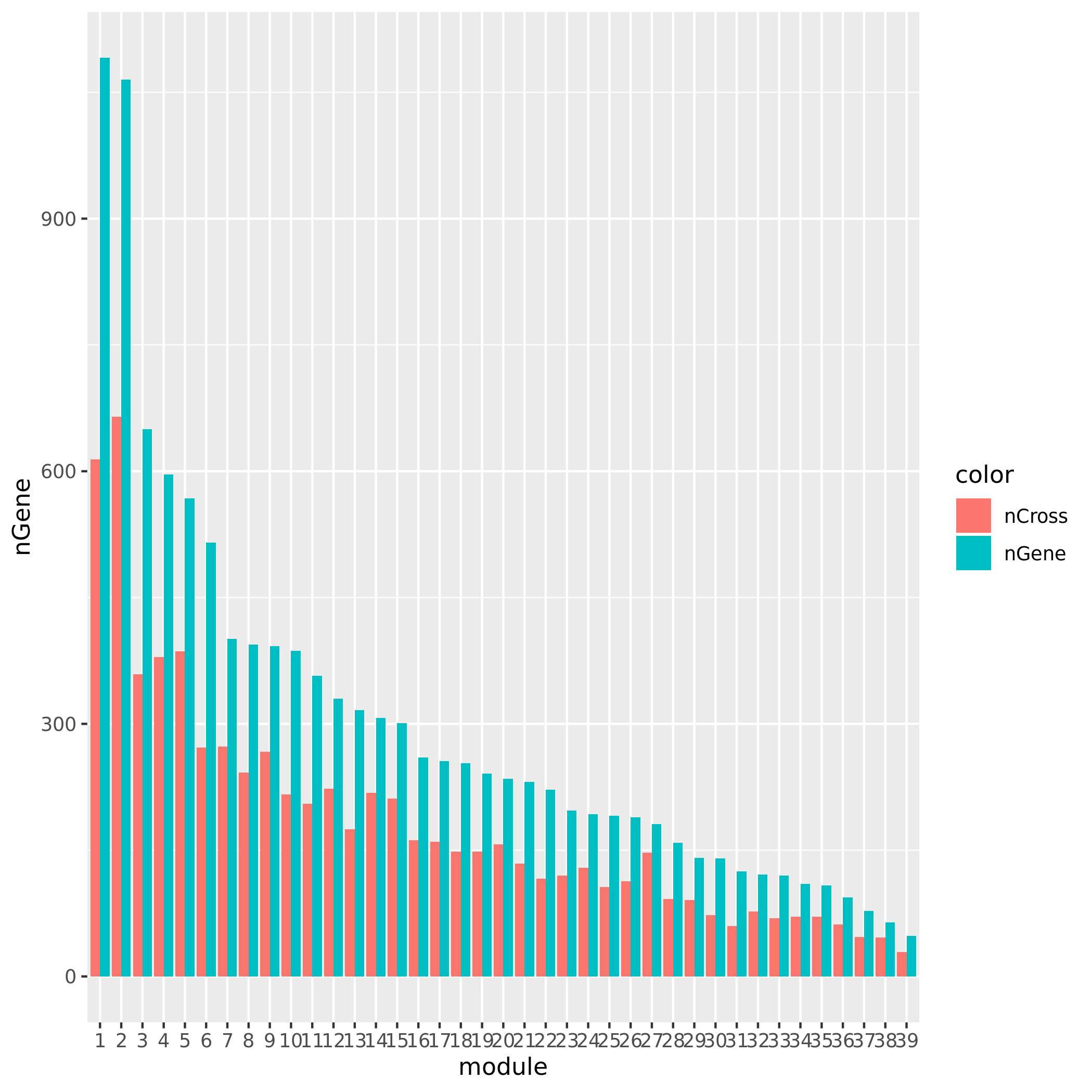
+ Check if the signals' nearby genes are cross-mapped with genes in their corresponding module. The signal on chr5 corresponding to module8 has 20 genes +/- 500Kb away from its TSS. Many of them are crosspable with genes in the module 8. The number of of genes in the module crossmapped with each of the 20 genes are: `1, 144, 0, 62, 54, 0, 63, 4, 0, 0, 0, 59, 145, 0, 0, 128, 0, 23, 53`, where the nearest gene is crossmappable with 1 gene in the module.The other signals on chr1, chr16, and chr5:47210790 don’t have any nearby genes around its TSS.
See the following plot for number of cross-mapped genes in each module.
| Version | Author | Date |
|---|---|---|
| d22021e | Lili Wang | 2021-01-19 |
New TCGA by the standard filtering
eQTLGen
eQTLGen description
This full dataset includes 19942 genes that showed expression in blood tested and 10317 SNPs that are trait-associated SNPs based on GWAS Catalog.
After gene filter steps described in
Dec 10, there are 4963 genes left. Applying the same filtering to 13634 DGN genes, there are 3695 genes left, among which 3642 are also included in eQTLGen. So, I will use these genes to do the downstream analysis, e.g. constructing co-expressed gene modules. These 3642 genes result in 19 gene modules.Replication of DGN signals in eQTLGen
The table below gives the signals found in eQTLGen and DGN.
The first two rows give results based on eQTLGen zscores, with row 1 using
qvaluefor FDR correction (threshold \(0.05\)) and row 2 using \(\frac{0.05}{\#DGN signals}\) as significance threshold. The third row is based on the same gene modules and SNPs but tensorQTL zscores using DGN expression data. The FDR correction uses the empirical distribution of pvalues from the combined chr’s and modules (10 permutations).
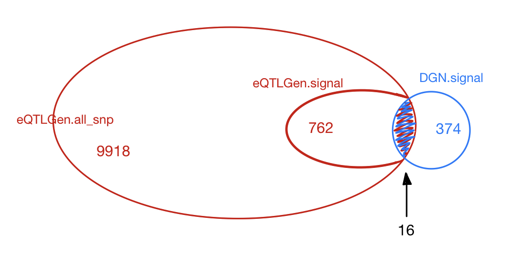
| Dataset | FDR | minp | (QTL, module) | unique QTL | independent QTL |
|---|---|---|---|---|---|
| eQTLGen | qvalue | 5.82e-04 | 2195 | 909 | 348 |
| eQTLGen | 0.05/#DGN signals | 1.18e-04 | 1707 | 762 | 286 |
| eQTLGen_DGN | combined chr+module #10-perms | 1.00e-07 | 420 | 374 | 28 |
Among 374 eQTLGen_DGN signals, 16 are replicated in 762 eQTLGen signals. These 16 replicated signals consists of 6 independent SNPs, including (based on GRCh37),
- rs12485738 : 3:56865776, intron variant of ARHGEF3.
- rs643381 : 6:139839423. (rs590856, 6:139844429).
- rs149007767 7:50370254: , intron variant of IKZF1.
- rs12718597 : 7:50428428, intron variant of IKZF1.
- rs35979828 : 12:54685880, 500B downstream variant of NFE2.
- rs7210990 : 17:16170764, intron variant of PIGL.
- Replication of DGN signals in eQTLGen
DGN
| Version | Author | Date |
|---|---|---|
| 60cf10e | Lili Wang | 2021-01-17 |
R version 4.1.0 (2021-05-18)
Platform: x86_64-apple-darwin17.0 (64-bit)
Running under: macOS Catalina 10.15.6

Matrix products: default
BLAS:   /Library/Frameworks/R.framework/Versions/4.1/Resources/lib/libRblas.dylib
LAPACK: /Library/Frameworks/R.framework/Versions/4.1/Resources/lib/libRlapack.dylib

locale:
[1] en_US.UTF-8/en_US.UTF-8/en_US.UTF-8/C/en_US.UTF-8/en_US.UTF-8

attached base packages:
[1] stats     graphics  grDevices utils     datasets  methods   base

other attached packages:
[1] data.table_1.14.0 workflowr_1.6.2

loaded via a namespace (and not attached):
 [1] Rcpp_1.0.6        whisker_0.4       knitr_1.33        magrittr_2.0.1
 [5] R6_2.5.0          rlang_0.4.11      fansi_0.5.0       highr_0.9
 [9] stringr_1.4.0     tools_4.1.0       xfun_0.23         utf8_1.2.1
[13] git2r_0.28.0      htmltools_0.5.1.1 ellipsis_0.3.2    rprojroot_2.0.2
[17] yaml_2.2.1        digest_0.6.27     tibble_3.1.2      lifecycle_1.0.0
[21] crayon_1.4.1      later_1.2.0       vctrs_0.3.8       promises_1.2.0.1
[25] fs_1.5.0          glue_1.4.2        evaluate_0.14     rmarkdown_2.8
[29] stringi_1.6.2     compiler_4.1.0    pillar_1.6.1      httpuv_1.6.1
[33] pkgconfig_2.0.3