Metabolite composition
Last updated: 2020-12-11
Checks: 7 0
Knit directory: exp_evol_respiration/
This reproducible R Markdown analysis was created with workflowr (version 1.6.2). The Checks tab describes the reproducibility checks that were applied when the results were created. The Past versions tab lists the development history.
Great! Since the R Markdown file has been committed to the Git repository, you know the exact version of the code that produced these results.
Great job! The global environment was empty. Objects defined in the global environment can affect the analysis in your R Markdown file in unknown ways. For reproduciblity it’s best to always run the code in an empty environment.
The command set.seed(20190703) was run prior to running the code in the R Markdown file. Setting a seed ensures that any results that rely on randomness, e.g. subsampling or permutations, are reproducible.
Great job! Recording the operating system, R version, and package versions is critical for reproducibility.
Nice! There were no cached chunks for this analysis, so you can be confident that you successfully produced the results during this run.
Great job! Using relative paths to the files within your workflowr project makes it easier to run your code on other machines.
Great! You are using Git for version control. Tracking code development and connecting the code version to the results is critical for reproducibility.
The results in this page were generated with repository version 9d65fc7. See the Past versions tab to see a history of the changes made to the R Markdown and HTML files.
Note that you need to be careful to ensure that all relevant files for the analysis have been committed to Git prior to generating the results (you can use wflow_publish or wflow_git_commit). workflowr only checks the R Markdown file, but you know if there are other scripts or data files that it depends on. Below is the status of the Git repository when the results were generated:
Ignored files:
    Ignored:    .DS_Store
    Ignored:    .Rproj.user/
    Ignored:    analysis/.DS_Store

Unstaged changes:
    Modified:   output/brms_metabolite_SEM.rds
Note that any generated files, e.g. HTML, png, CSS, etc., are not included in this status report because it is ok for generated content to have uncommitted changes.
These are the previous versions of the repository in which changes were made to the R Markdown (analysis/metabolites.Rmd) and HTML (docs/metabolites.html) files. If you’ve configured a remote Git repository (see ?wflow_git_remote), click on the hyperlinks in the table below to view the files as they were in that past version.
| File | Version | Author | Date | Message |
|---|---|---|---|---|
| Rmd | 9d65fc7 | lukeholman | 2020-12-11 | Tweaks |
| html | 2911fb9 | lukeholman | 2020-12-10 | Build site. |
| Rmd | 184b0a4 | lukeholman | 2020-12-10 | Tweaks |
| html | a361e42 | lukeholman | 2020-12-10 | Build site. |
| Rmd | 98c43b5 | lukeholman | 2020-12-10 | Tweaks |
| html | 7fca240 | lukeholman | 2020-12-10 | Build site. |
| Rmd | 125d4a2 | lukeholman | 2020-12-10 | Tweaks |
| html | 31ed22a | lukeholman | 2020-12-10 | Build site. |
| Rmd | 8464a7f | lukeholman | 2020-12-10 | Tweaks |
| html | 901053c | lukeholman | 2020-12-10 | Build site. |
| Rmd | 904af31 | lukeholman | 2020-12-10 | Tweaks |
| html | f7c88a2 | lukeholman | 2020-12-10 | Build site. |
| Rmd | 68780f6 | lukeholman | 2020-12-10 | Tweaks |
| html | deb7183 | lukeholman | 2020-12-09 | Build site. |
| Rmd | 720eb6d | lukeholman | 2020-12-09 | Tweaks |
| html | b731971 | lukeholman | 2020-12-09 | Build site. |
| Rmd | 398d963 | lukeholman | 2020-12-09 | Tweaks |
| html | b449eb3 | lukeholman | 2020-12-09 | Build site. |
| Rmd | 15f3c92 | lukeholman | 2020-12-09 | Tweaks |
| html | 43cc270 | lukeholman | 2020-12-09 | Build site. |
| Rmd | 2642c27 | lukeholman | 2020-12-09 | More work |
| html | 4f5ee28 | lukeholman | 2020-12-04 | Build site. |
| Rmd | d441b69 | lukeholman | 2020-12-04 | Luke metabolites analysis |
| Rmd | c8feb2d | lukeholman | 2020-11-30 | Same page with Martin |
| html | 3fdbcb2 | lukeholman | 2020-11-30 | Tweaks Nov 2020 |
Load packages
library(tidyverse)
library(GGally)
library(gridExtra)
library(ggridges)
library(brms)
library(tidybayes)
library(DT)
library(kableExtra)
library(knitrhooks) # install with devtools::install_github("nathaneastwood/knitrhooks")
output_max_height() # a knitrhook option

options(stringsAsFactors = FALSE)
Load metabolite composition data
This analysis set out to test whether sexual selection treatment had an effect on metabolite composition of flies. We measured fresh and dry fly weight in milligrams, plus the weights of five metabolites which together equal the dry weight. These are:
Lipid_conc(i.e. the weight of the hexane fraction, divided by the full dry weight),Carbohydrate_conc(i.e. the weight of the aqueous fraction, divided by the full dry weight),Protein_conc(i.e. \(\mu\)g of protein per milligram as measured by the bicinchoninic acid protein assay),Glycogen_conc(i.e. \(\mu\)g of glycogen per milligram as measured by the hexokinase assay), andChitin_conc(estimated as the difference between the initial and final dry weights)
We expect body weight to vary between the sexes and potentially between treatments. In turn, we expect body weight to affect our five response variables of interest. Larger flies will have more lipids, carbs, etc., and this may vary by sex and treatment both directly and indirectly.
metabolites <- read_csv('data/3.metabolite_data.csv') %>%
  mutate(sex = ifelse(sex == "m", "Male", "Female"),
         line = paste(treatment, line, sep = ""),
         treatment = ifelse(treatment == "M", "Monogamy", "Polyandry")) %>%
  # log transform glycogen since it shows a long tail (others are reasonably normal-looking)
  mutate(Glycogen_ug_mg = log(Glycogen_ug_mg)) %>%
  # There was a technical error with flies collected on day 1,
  # so they are excluded from the whole paper. All the measurements analysed are of 3d-old flies
  filter(time == '2') %>%
  select(-time)

scaled_metabolites <- metabolites %>%
  # Find proportional metabolites as a proportion of total dry weight
  mutate(
    Dry_weight = dwt_mg,
    Lipid_conc = Hex_frac / Dry_weight,
    Carbohydrate_conc = Aq_frac / Dry_weight,
    Protein_conc = Protein_ug_mg,
    Glycogen_conc = Glycogen_ug_mg,
    Chitin_conc = Chitin_mg_mg) %>%
  select(sex, treatment, line, Dry_weight, ends_with("conc")) %>%
  mutate_at(vars(ends_with("conc")), ~ as.numeric(scale(.x))) %>%
  mutate(Dry_weight = as.numeric(scale(Dry_weight))) %>%
  mutate(sextreat = paste(sex, treatment),
         sextreat = replace(sextreat, sextreat == "Male Monogamy", "M males"),
         sextreat = replace(sextreat, sextreat == "Male Polyandry", "P males"),
         sextreat = replace(sextreat, sextreat == "Female Monogamy", "M females"),
         sextreat = replace(sextreat, sextreat == "Female Polyandry", "P females"),
         sextreat = factor(sextreat, c("M males", "P males", "M females", "P females")))
Inspect the raw data
Raw numbers
All variables are shown in standard units (i.e. mean = 0, SD = 1).
my_data_table <- function(df){
  datatable(
    df, rownames=FALSE,
    autoHideNavigation = TRUE,
    extensions = c("Scroller",  "Buttons"),
    options = list(
      dom = 'Bfrtip',
      deferRender=TRUE,
      scrollX=TRUE, scrollY=400,
      scrollCollapse=TRUE,
      buttons =
        list('csv', list(
          extend = 'pdf',
          pageSize = 'A4',
          orientation = 'landscape',
          filename = 'Apis_methylation')),
      pageLength = 50
    )
  )
}

scaled_metabolites %>%
  select(-sextreat) %>%
  mutate_if(is.numeric, ~ format(round(.x, 3), nsmall = 3)) %>%
  my_data_table()
Simple plots
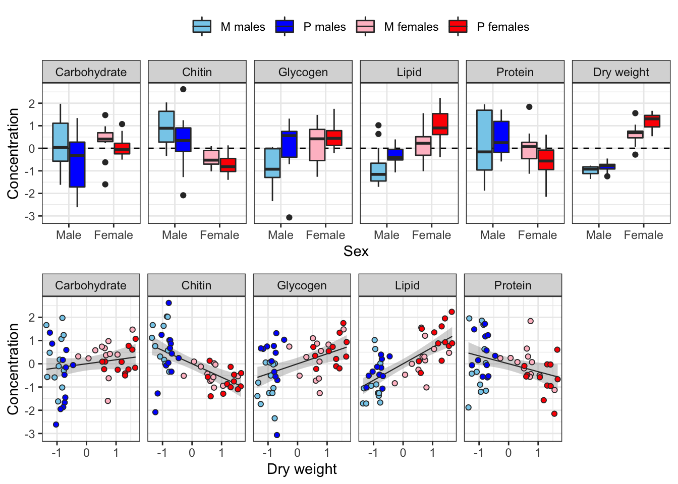
The following plot shows how each metabolite varies between sexes and treatments, and how the consecration of each metabolite co-varies with dry weight across individuals.
levels <- c("Carbohydrate", "Chitin", "Glycogen", "Lipid", "Protein", "Dry weight")

cols <- c("M females" = "pink",
          "P females" = "red",
          "M males" = "skyblue",
          "P males" = "blue")

grid.arrange(
  scaled_metabolites %>%
    rename_all(~ str_remove_all(.x, "_conc")) %>%
    rename(`Dry weight` = Dry_weight) %>%
    mutate(sex = factor(sex, c("Male", "Female"))) %>%
    reshape2::melt(id.vars = c('sex', 'treatment', 'sextreat', 'line')) %>%
    mutate(variable = factor(variable, levels)) %>%
    ggplot(aes(x = sex, y = value,  fill  = sextreat)) +
    geom_hline(yintercept = 0, linetype = 2) +
    geom_boxplot() +
    facet_grid( ~ variable) +
    theme_bw() +
    xlab("Sex") + ylab("Concentration") +
    theme(legend.position = 'top') +
    scale_fill_manual(values = cols, name = ""),

  arrangeGrob(
    scaled_metabolites %>%
      rename_all(~ str_remove_all(.x, "_conc")) %>%
      reshape2::melt(id.vars = c('sex', 'treatment', 'sextreat', 'line', 'Dry_weight')) %>%
      mutate(variable = factor(variable, levels)) %>%
      ggplot(aes(x = Dry_weight, y = value, colour = sextreat, fill = sextreat)) +
      geom_smooth(method = 'lm', se = TRUE, aes(colour = NULL, fill = NULL), colour = "grey20", size = .4) +
      geom_point(pch = 21, colour = "grey20") +
      facet_grid( ~ variable) +
      theme_bw() +
      xlab("Dry weight") + ylab("Concentration") +
      theme(legend.position = 'none') +
      scale_colour_manual(values = cols, name = "") +
      scale_fill_manual(values = cols, name = ""),
    scaled_metabolites %>%
      rename_all(~ str_remove_all(.x, "_conc")) %>%
      reshape2::melt(id.vars = c('sex', 'treatment', 'sextreat', 'line', 'Dry_weight')) %>%
      mutate(variable = factor(variable, levels)) %>%
      ggplot(aes(x = Dry_weight, y = value, colour = sextreat, fill = sextreat)) +
      theme_void() + ylab(NULL), nrow = 1, widths = c(0.84, 0.16)),
  heights = c(0.55, 0.45)
)
Plot of correlations between variables
Some of the metabolites, especially lipid concentration, are correlated with dry weight. There is also a large difference in dry weight between sexes (and treatments, to a less extent), and sex and treatment effects are evident for some of the metabolites in the raw data. Some of the metabolites are weakly correlated with other metabolites, e.g. lipid and glycogen concentration.
modified_densityDiag <- function(data, mapping, ...) {
  ggally_densityDiag(data, mapping, colour = "grey10", ...) +
    scale_fill_manual(values = cols) +
  scale_x_continuous(guide = guide_axis(check.overlap = TRUE))
}

modified_points <- function(data, mapping, ...) {
  ggally_points(data, mapping, pch = 21, colour = "grey10", ...) +
    scale_fill_manual(values = cols) +
    scale_x_continuous(guide = guide_axis(check.overlap = TRUE))
}

modified_facetdensity <- function(data, mapping, ...) {
  ggally_facetdensity(data, mapping, ...) +
    scale_colour_manual(values = cols)
}

modified_box_no_facet <- function(data, mapping, ...) {
  ggally_box_no_facet(data, mapping, colour = "grey10", ...) +
    scale_fill_manual(values = cols)
}

pairs_plot <- scaled_metabolites %>%
  arrange(sex, treatment) %>%
  select(-line, -sex, -treatment) %>%
  rename(`Sex and treatment` = sextreat) %>%
  rename_all(~ str_replace_all(.x, "_", " ")) %>%
  ggpairs(aes(colour = `Sex and treatment`, fill = `Sex and treatment`),
          diag = list(continuous = wrap(modified_densityDiag, alpha = 0.7),
                      discrete = wrap("blank")),
          lower = list(continuous = wrap(modified_points, alpha = 0.7, size = 1.1),
                       discrete = wrap("blank"),
                       combo = wrap(modified_box_no_facet, alpha = 0.7)),
          upper = list(continuous = wrap(modified_points, alpha = 0.7, size = 1.1),
                       discrete = wrap("blank"),
                       combo = wrap(modified_box_no_facet, alpha = 0.7, size = 0.5)))
pairs_plot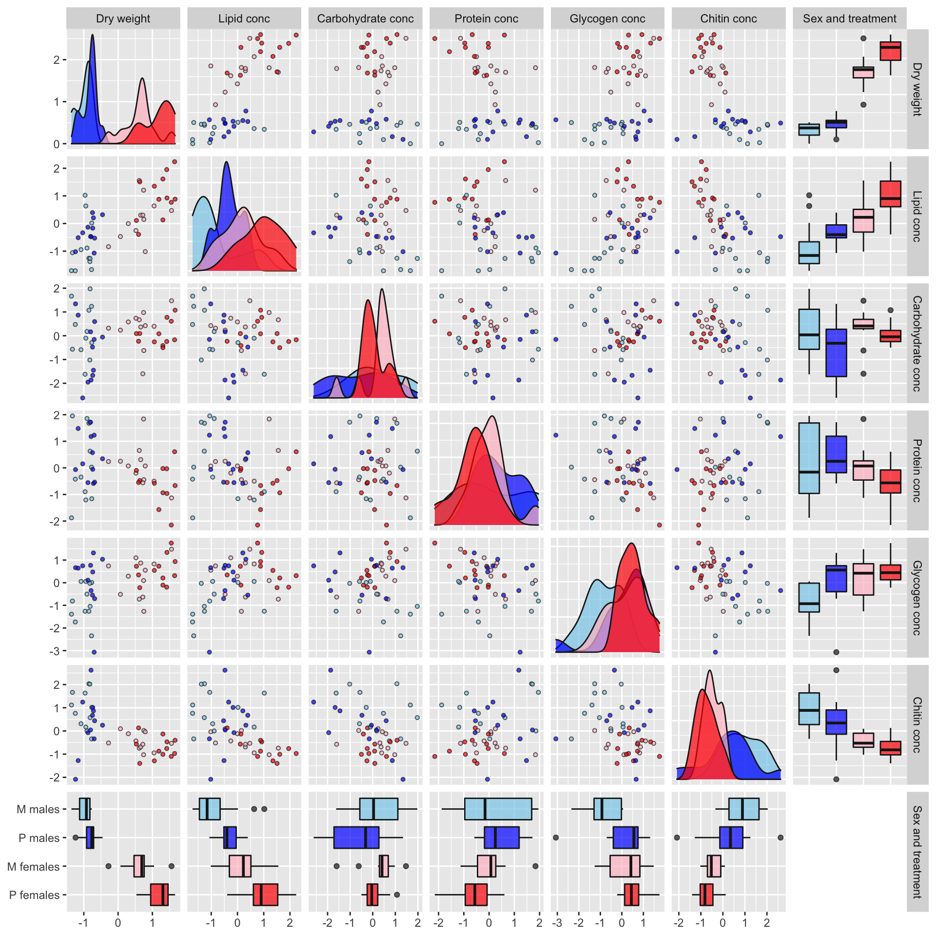
| Version | Author | Date |
|---|---|---|
| 43cc270 | lukeholman | 2020-12-09 |
Mean dry weight
se <- function(x) sd(x) / sqrt(length(x))
metabolites %>%
  group_by(sex, treatment) %>%
  summarise(mean_dwt = mean(dwt_mg),
            SE = se(dwt_mg),
            n = n()) %>%
kable(digits = 3) %>% kable_styling(full_width = FALSE)| sex | treatment | mean_dwt | SE | n |
|---|---|---|---|---|
| Female | Monogamy | 0.562 | 0.019 | 12 |
| Female | Polyandry | 0.644 | 0.017 | 12 |
| Male | Monogamy | 0.330 | 0.009 | 12 |
| Male | Polyandry | 0.353 | 0.009 | 12 |
Directed acyclic graph (DAG)
This directed acyclic graph (DAG) illustrates the causal pathways that we observed between the experimental or measured variables (square boxes) and latent variables (ovals). We hypothesise that sex and mating system potentially influence dry weight as well as the metabolite composition (which we assessed by estimating the concentrations of carbohydrates, chitin, glycogen, lipids and protein). Additionally, dry weight is likely correlated with metabolite composition, and so dry weight acts as a ‘mediator variable’ between metabolite composition, and sex and treatment. The structural equation model below is built with this DAG in mind.
DiagrammeR::grViz('digraph {

graph [layout = dot, rankdir = LR]

# define the global styles of the nodes. We can override these in box if we wish
node [shape = rectangle, style = filled, fillcolor = Linen]

"Metabolite\ncomposition" [shape = oval, fillcolor = Beige]

# edge definitions with the node IDs
"Mating system\ntreatment (M vs P)" -> {"Dry weight"}
"Mating system\ntreatment (M vs P)" -> {"Metabolite\ncomposition"}

"Sex\n(Female vs Male)" -> {"Dry weight"} -> {"Metabolite\ncomposition"}
"Sex\n(Female vs Male)" -> {"Metabolite\ncomposition"}

{"Metabolite\ncomposition"} -> "Carbohydrates"
{"Metabolite\ncomposition"} -> "Chitin"
{"Metabolite\ncomposition"} -> "Glycogen"
{"Metabolite\ncomposition"} -> "Lipids"
{"Metabolite\ncomposition"} -> "Protein"
}')
Fit brms structural equation model
Here we fit a model of the five metabolites, which includes dry body weight as a mediator variable. That is, our model estimates the effect of treatment, sex and line (and all the 2- and 3-way interactions) on dry weight, and then estimates the effect of those some predictors (plus dry weight) on the five metabolites. The model assumes that although the different sexes, treatment groups, and lines may differ in their dry weight, the relationship between dry weight and the metabolites does not vary by sex/treatment/line. This assumption was made to constrain the number of parameters in the model, and to reflect out prior beliefs about allometric scaling of metabolites.
Define Priors
We use set fairly tight Normal priors on all fixed effect parameters, which ‘regularises’ the estimates towards zero – this is conservative (because it ensures that a stronger signal in the data is needed to produce a given posterior effect size estimate), and it also helps the model to converge. Similarly, we set a somewhat conservative half-cauchy prior (mean 0, scale 0.01) on the random effects for line (i.e. we consider large differences between lines – in terms of means and treatment effects – to be possible but improbable). We leave all other priors at the defaults used by brms. Note that the Normal priors are slightly wider in the model of dry weight, because we expect larger effect sizes of sex and treatment on dry weight than on the metabolite composition.
prior1 <- c(set_prior("normal(0, 0.5)", class = "b", resp = 'Lipid'),
            set_prior("normal(0, 0.5)", class = "b", resp = 'Carbohydrate'),
            set_prior("normal(0, 0.5)", class = "b", resp = 'Protein'),
            set_prior("normal(0, 0.5)", class = "b", resp = 'Glycogen'),
            set_prior("normal(0, 0.5)", class = "b", resp = 'Chitin'),
            set_prior("normal(0, 1)", class = "b", resp = 'Dryweight'),
            set_prior("cauchy(0, 0.01)", class = "sd", resp = 'Lipid', group = "line"),
            set_prior("cauchy(0, 0.01)", class = "sd", resp = 'Carbohydrate', group = "line"),
            set_prior("cauchy(0, 0.01)", class = "sd", resp = 'Protein', group = "line"),
            set_prior("cauchy(0, 0.01)", class = "sd", resp = 'Glycogen', group = "line"),
            set_prior("cauchy(0, 0.01)", class = "sd", resp = 'Chitin', group = "line"),
            set_prior("cauchy(0, 0.01)", class = "sd", resp = 'Dryweight', group = "line"))

prior1
prior class coef group resp dpar nlpar bound source
normal(0, 0.5) b Lipid user
normal(0, 0.5) b Carbohydrate user
normal(0, 0.5) b Protein user
normal(0, 0.5) b Glycogen user
normal(0, 0.5) b Chitin user
normal(0, 1) b Dryweight user
cauchy(0, 0.01) sd line Lipid user
cauchy(0, 0.01) sd line Carbohydrate user
cauchy(0, 0.01) sd line Protein user
cauchy(0, 0.01) sd line Glycogen user
cauchy(0, 0.01) sd line Chitin user
cauchy(0, 0.01) sd line Dryweight user
Define the six sub-models
The fixed effects formula is sex * treatment + Dryweight (or sex * treatment in the case of the model of dry weight). The random effects part of the formula indicates that the 8 independent selection lines may differ in their means, and that the treatment effect may vary in sign/magnitude between lines. The notation | p | means that the model estimates the correlations in line effects (both slopes and intercepts) between the 6 response variables. Finally, the notation set_rescor(TRUE) means that the model should estimate the residual correlations between the response variables.
brms_formula <-

  # Sub-models of the 5 metabolites
  bf(mvbind(Lipid, Carbohydrate, Protein, Glycogen, Chitin) ~
       sex*treatment + Dryweight + (treatment | p | line)) +

  # dry weight sub-model
   bf(Dryweight ~ sex*treatment + (treatment | p | line)) +

  # Allow for (and estimate) covariance between the residuals of the difference response variables
  set_rescor(TRUE)

brms_formula
Lipid ~ sex * treatment + Dryweight + (treatment | p | line) Carbohydrate ~ sex * treatment + Dryweight + (treatment | p | line) Protein ~ sex * treatment + Dryweight + (treatment | p | line) Glycogen ~ sex * treatment + Dryweight + (treatment | p | line) Chitin ~ sex * treatment + Dryweight + (treatment | p | line) Dryweight ~ sex * treatment + (treatment | p | line)
Running the model
The model is run over 4 chains with 5000 iterations each (with the first 2500 discarded as burn-in), for a total of 2500*4 = 10,000 posterior samples.
if(!file.exists("output/brms_metabolite_SEM.rds")){
  brms_metabolite_SEM <- brm(
    brms_formula,
    data = scaled_metabolites %>% # brms does not like underscores in variable names
      rename(Dryweight = Dry_weight) %>%
      rename_all(~ gsub("_conc", "", .x)),
    iter = 5000, chains = 4, cores = 1,
    prior = prior1,
    control = list(max_treedepth = 20,
                   adapt_delta = 0.99)
  )

  saveRDS(brms_metabolite_SEM, "output/brms_metabolite_SEM.rds")
} else {
  brms_metabolite_SEM <- readRDS('output/brms_metabolite_SEM.rds')
}
Posterior predictive check of model fit
The plot below shows that the fitted model is able to produce posterior predictions that have a similar distribution to the original data, for each of the response variables, which is a necessary condition for the model to be used for statistical inference.
grid.arrange(
  pp_check(brms_metabolite_SEM, resp = "Dryweight") +
    ggtitle("Dry weight") + theme(legend.position = "none"),
  pp_check(brms_metabolite_SEM, resp = "Lipid") +
    ggtitle("Lipid") + theme(legend.position = "none"),
  pp_check(brms_metabolite_SEM, resp = "Carbohydrate") +
    ggtitle("Carbohydrate") + theme(legend.position = "none"),
  pp_check(brms_metabolite_SEM, resp = "Protein") +
    ggtitle("Protein") + theme(legend.position = "none"),
  pp_check(brms_metabolite_SEM, resp = "Glycogen") +
    ggtitle("Glycogen") + theme(legend.position = "none"),
  pp_check(brms_metabolite_SEM, resp = "Chitin") +
    ggtitle("Chitin") + theme(legend.position = "none"),
  nrow = 2
)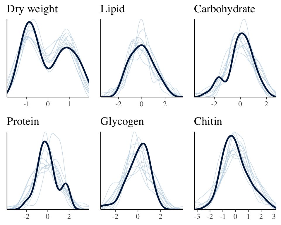
Table of model parameter estimates
Formatted table
This tables shows the fixed effects estimates for the treatment, sex, their interaction, as well as the slope associated with dry weight (where relevant), for each of the six response variables. The p column shows 1 - minus the “probability of direction”, i.e. the posterior probability that the reported sign of the estimate is correct given the data and the prior; subtracting this value from one gives a Bayesian equivalent of a one-sided p-value. For brevity, we have omitted all the parameter estimates involving the predictor variable line, as well as the estimates of residual (co)variance. Click the next tab to see a complete summary of the model and its output.
vars <- c("Lipid", "Carbohydrate", "Glycogen", "Protein", "Chitin")
tests <- c('_Dryweight', '_sexMale',
           '_sexMale:treatmentPolyandry',
           '_treatmentPolyandry')

hypSEM <- data.frame(expand_grid(vars, tests) %>%
                       mutate(est = NA,
                              err = NA,
                              lwr = NA,
                              upr = NA) %>%
                       # bind body weight on the end
                       rbind(data.frame(
                         vars = rep('Dryweight', 3),
                         tests = c('_sexMale',
                                   '_treatmentPolyandry',
                                   '_sexMale:treatmentPolyandry'),
                         est = NA,
                         err = NA,
                         lwr = NA,
                         upr = NA)))

for(i in 1:nrow(hypSEM)) {

  result = hypothesis(brms_metabolite_SEM,
                      paste0(hypSEM[i, 1], hypSEM[i, 2], ' = 0'))$hypothesis

  hypSEM[i, 3] = round(result$Estimate, 3)
  hypSEM[i, 4] = round(result$Est.Error, 3)
  hypSEM[i, 5] = round(result$CI.Lower, 3)
  hypSEM[i, 6] = round(result$CI.Upper, 3)

}

pvals <- bayestestR::p_direction(brms_metabolite_SEM) %>%
  as.data.frame() %>%
  mutate(vars = map_chr(str_split(Parameter, "_"), ~ .x[2]),
         tests = map_chr(str_split(Parameter, "_"), ~ .x[3]),
         tests = str_c("_", str_remove_all(tests, "[.]")),
         tests = replace(tests, tests == "_sexMaletreatmentPolyandry", "_sexMale:treatmentPolyandry")) %>%
  filter(!str_detect(tests, "line")) %>%
  mutate(p_val = 1 - pd, star = ifelse(p_val < 0.05, "\\*", "")) %>%
  select(vars, tests, p_val, star)


hypSEM <- hypSEM %>% left_join(pvals, by = c("vars", "tests"))

hypSEM  %>%
  mutate(Parameter = c(rep(c('Dry weight', 'Sex (M)',
                             'Sex (M) x Treatment (P)',
                             'Treatment (P)'), 5),
                       'Sex (M)', 'Treatment (P)', 'Sex (M) x Treatment (P)'))  %>%
  mutate(Parameter = factor(Parameter, c("Dry weight", "Sex (M)", "Treatment (P)", "Sex (M) x Treatment (P)")),
         vars = factor(vars, c("Carbohydrate", "Chitin", "Glycogen", "Lipid", "Protein", "Dryweight"))) %>%
  arrange(vars, Parameter) %>%
  select(Parameter, Estimate = est, `Est. error` = err,
         `CI lower` = lwr, `CI upper` = upr, `p` = p_val, star) %>%
  rename(` ` = star) %>%
  kable() %>%
  kable_styling(full_width = FALSE) %>%
  group_rows("Carbohydrates", 1, 4) %>%
  group_rows("Chitin", 5, 8) %>%
  group_rows("Glycogen", 9, 12) %>%
  group_rows("Lipids", 13, 16) %>%
  group_rows("Protein", 17, 20) %>%
group_rows("Dry weight", 21, 23)| Parameter | Estimate | Est. error | CI lower | CI upper | p | |
|---|---|---|---|---|---|---|
| Carbohydrates | ||||||
| Dry weight | 0.098 | 0.269 | -0.432 | 0.626 | 0.3544 | |
| Sex (M) | 0.016 | 0.423 | -0.814 | 0.849 | 0.4847 | |
| Treatment (P) | -0.245 | 0.302 | -0.834 | 0.353 | 0.2049 | |
| Sex (M) x Treatment (P) | -0.418 | 0.350 | -1.095 | 0.269 | 0.1189 | |
| Chitin | ||||||
| Dry weight | -0.483 | 0.263 | -1.001 | 0.030 | 0.0324 | * |
| Sex (M) | 0.400 | 0.428 | -0.440 | 1.227 | 0.1722 | |
| Treatment (P) | -0.115 | 0.283 | -0.667 | 0.456 | 0.3355 | |
| Sex (M) x Treatment (P) | -0.316 | 0.327 | -0.953 | 0.324 | 0.1683 | |
| Glycogen | ||||||
| Dry weight | 0.334 | 0.266 | -0.187 | 0.854 | 0.1066 | |
| Sex (M) | -0.270 | 0.423 | -1.094 | 0.560 | 0.2596 | |
| Treatment (P) | 0.219 | 0.294 | -0.366 | 0.795 | 0.2241 | |
| Sex (M) x Treatment (P) | 0.391 | 0.349 | -0.305 | 1.065 | 0.1340 | |
| Lipids | ||||||
| Dry weight | 0.543 | 0.255 | 0.041 | 1.041 | 0.0180 | * |
| Sex (M) | -0.109 | 0.411 | -0.915 | 0.692 | 0.3932 | |
| Treatment (P) | 0.388 | 0.273 | -0.157 | 0.916 | 0.0742 | |
| Sex (M) x Treatment (P) | -0.052 | 0.308 | -0.640 | 0.557 | 0.4311 | |
| Protein | ||||||
| Dry weight | -0.216 | 0.267 | -0.743 | 0.301 | 0.2086 | |
| Sex (M) | -0.019 | 0.428 | -0.860 | 0.808 | 0.4831 | |
| Treatment (P) | -0.212 | 0.306 | -0.801 | 0.394 | 0.2456 | |
| Sex (M) x Treatment (P) | 0.344 | 0.363 | -0.371 | 1.050 | 0.1706 | |
| Dry weight | ||||||
| Sex (M) | -1.613 | 0.141 | -1.892 | -1.341 | 0.0000 | * |
| Treatment (P) | 0.528 | 0.159 | 0.217 | 0.839 | 0.0015 | * |
| Sex (M) x Treatment (P) | -0.359 | 0.198 | -0.748 | 0.029 | 0.0354 | * |
Complete output from summary.brmsfit()
- ‘Group-Level Effects’ (also called random effects): This shows the (co)variances associated with the line-specific intercepts (which have names like
sd(Lipid_Intercept)) and slopes (e.g.sd(Dryweight_treatmentPolyandry)), as well as the correlations between these effects (e.g.cor(Lipid_Intercept,Protein_Intercept)is the correlation in line effects on lipids and proteins) - ‘Population-Level Effects:’ (also called fixed effects): These give the estimates of the intercept (i.e. for female M flies) and the effects of treatment, sex, dry weight, and the treatment \(\times\) sex interaction, for each response variable.
- ‘Family Specific Parameters’: This is the parameter sigma for the residual variance for each response variable
- ‘Residual Correlations:’ This give the correlations between the residuals for each pairs of response variables.
Note that the model has converged (Rhat = 1) and the posterior is adequately samples (high ESS values).
brms_metabolite_SEM Family: MV(gaussian, gaussian, gaussian, gaussian, gaussian, gaussian)
Links: mu = identity; sigma = identity
mu = identity; sigma = identity
mu = identity; sigma = identity
mu = identity; sigma = identity
mu = identity; sigma = identity
mu = identity; sigma = identity
Formula: Lipid ~ sex * treatment + Dryweight + (treatment | p | line)
Carbohydrate ~ sex * treatment + Dryweight + (treatment | p | line)
Protein ~ sex * treatment + Dryweight + (treatment | p | line)
Glycogen ~ sex * treatment + Dryweight + (treatment | p | line)
Chitin ~ sex * treatment + Dryweight + (treatment | p | line)
Dryweight ~ sex * treatment + (treatment | p | line)
Data: scaled_metabolites %>% rename(Dryweight = Dry_weig (Number of observations: 48)
Samples: 4 chains, each with iter = 5000; warmup = 2500; thin = 1;
total post-warmup samples = 10000
Group-Level Effects:
~line (Number of levels: 8)
Estimate Est.Error l-95% CI u-95% CI Rhat Bulk_ESS Tail_ESS
sd(Lipid_Intercept) 0.09 0.15 0.00 0.52 1.00 2205 3122
sd(Lipid_treatmentPolyandry) 0.03 0.09 0.00 0.26 1.00 10416 5634
sd(Carbohydrate_Intercept) 0.07 0.14 0.00 0.49 1.00 4009 3563
sd(Carbohydrate_treatmentPolyandry) 0.05 0.14 0.00 0.47 1.00 6147 3091
sd(Protein_Intercept) 0.05 0.12 0.00 0.46 1.00 5474 3122
sd(Protein_treatmentPolyandry) 0.03 0.07 0.00 0.23 1.00 14351 6537
sd(Glycogen_Intercept) 0.03 0.07 0.00 0.23 1.00 11763 5625
sd(Glycogen_treatmentPolyandry) 0.03 0.06 0.00 0.17 1.00 17080 6554
sd(Chitin_Intercept) 0.07 0.13 0.00 0.45 1.00 4045 3642
sd(Chitin_treatmentPolyandry) 0.04 0.10 0.00 0.32 1.00 10529 5452
sd(Dryweight_Intercept) 0.05 0.07 0.00 0.26 1.00 3499 4233
sd(Dryweight_treatmentPolyandry) 0.03 0.05 0.00 0.18 1.00 9771 6085
cor(Lipid_Intercept,Lipid_treatmentPolyandry) 0.00 0.28 -0.53 0.53 1.00 21961 6563
cor(Lipid_Intercept,Carbohydrate_Intercept) 0.01 0.28 -0.53 0.54 1.00 21503 6928
cor(Lipid_treatmentPolyandry,Carbohydrate_Intercept) -0.00 0.28 -0.52 0.52 1.00 13932 7502
cor(Lipid_Intercept,Carbohydrate_treatmentPolyandry) 0.00 0.28 -0.53 0.53 1.00 21292 7123
cor(Lipid_treatmentPolyandry,Carbohydrate_treatmentPolyandry) 0.00 0.28 -0.54 0.54 1.00 16111 7114
cor(Carbohydrate_Intercept,Carbohydrate_treatmentPolyandry) -0.00 0.28 -0.53 0.52 1.00 11393 7217
cor(Lipid_Intercept,Protein_Intercept) 0.00 0.27 -0.53 0.52 1.00 19726 6371
cor(Lipid_treatmentPolyandry,Protein_Intercept) 0.00 0.27 -0.51 0.52 1.00 15406 7396
cor(Carbohydrate_Intercept,Protein_Intercept) -0.00 0.28 -0.54 0.53 1.00 12967 6678
cor(Carbohydrate_treatmentPolyandry,Protein_Intercept) -0.00 0.28 -0.53 0.53 1.00 11298 7158
cor(Lipid_Intercept,Protein_treatmentPolyandry) 0.00 0.28 -0.53 0.54 1.00 20488 7090
cor(Lipid_treatmentPolyandry,Protein_treatmentPolyandry) 0.00 0.28 -0.53 0.54 1.00 15638 6415
cor(Carbohydrate_Intercept,Protein_treatmentPolyandry) 0.00 0.27 -0.52 0.53 1.00 12822 7402
cor(Carbohydrate_treatmentPolyandry,Protein_treatmentPolyandry) 0.01 0.27 -0.51 0.54 1.00 9969 6797
cor(Protein_Intercept,Protein_treatmentPolyandry) -0.00 0.28 -0.55 0.54 1.00 9096 7764
cor(Lipid_Intercept,Glycogen_Intercept) 0.01 0.28 -0.53 0.54 1.00 20387 6844
cor(Lipid_treatmentPolyandry,Glycogen_Intercept) 0.00 0.27 -0.52 0.52 1.00 15710 7288
cor(Carbohydrate_Intercept,Glycogen_Intercept) 0.00 0.27 -0.52 0.53 1.00 12027 7551
cor(Carbohydrate_treatmentPolyandry,Glycogen_Intercept) -0.00 0.28 -0.53 0.52 1.00 10155 6478
cor(Protein_Intercept,Glycogen_Intercept) -0.00 0.27 -0.53 0.53 1.00 8457 7573
cor(Protein_treatmentPolyandry,Glycogen_Intercept) -0.00 0.28 -0.53 0.53 1.00 7939 7545
cor(Lipid_Intercept,Glycogen_treatmentPolyandry) -0.00 0.28 -0.53 0.53 1.00 24265 6764
cor(Lipid_treatmentPolyandry,Glycogen_treatmentPolyandry) -0.00 0.28 -0.54 0.53 1.00 15931 6498
cor(Carbohydrate_Intercept,Glycogen_treatmentPolyandry) -0.00 0.27 -0.53 0.52 1.00 12481 7007
cor(Carbohydrate_treatmentPolyandry,Glycogen_treatmentPolyandry) -0.00 0.28 -0.54 0.53 1.00 10235 7304
cor(Protein_Intercept,Glycogen_treatmentPolyandry) -0.00 0.28 -0.54 0.53 1.00 9399 6972
cor(Protein_treatmentPolyandry,Glycogen_treatmentPolyandry) 0.00 0.28 -0.54 0.54 1.00 7546 6992
cor(Glycogen_Intercept,Glycogen_treatmentPolyandry) 0.00 0.28 -0.54 0.54 1.00 5830 6824
cor(Lipid_Intercept,Chitin_Intercept) -0.00 0.27 -0.54 0.52 1.00 18378 7300
cor(Lipid_treatmentPolyandry,Chitin_Intercept) -0.00 0.28 -0.53 0.53 1.00 15157 7133
cor(Carbohydrate_Intercept,Chitin_Intercept) -0.00 0.28 -0.54 0.54 1.00 12651 7259
cor(Carbohydrate_treatmentPolyandry,Chitin_Intercept) -0.00 0.28 -0.53 0.54 1.00 9382 7490
cor(Protein_Intercept,Chitin_Intercept) -0.00 0.27 -0.52 0.52 1.00 8910 7562
cor(Protein_treatmentPolyandry,Chitin_Intercept) -0.01 0.28 -0.54 0.52 1.00 8730 7568
cor(Glycogen_Intercept,Chitin_Intercept) 0.00 0.28 -0.53 0.55 1.00 6749 7815
cor(Glycogen_treatmentPolyandry,Chitin_Intercept) -0.00 0.28 -0.53 0.54 1.00 6389 7418
cor(Lipid_Intercept,Chitin_treatmentPolyandry) -0.00 0.28 -0.53 0.52 1.00 19844 6699
cor(Lipid_treatmentPolyandry,Chitin_treatmentPolyandry) -0.00 0.28 -0.54 0.53 1.00 15244 6811
cor(Carbohydrate_Intercept,Chitin_treatmentPolyandry) -0.00 0.27 -0.53 0.54 1.00 12465 7063
cor(Carbohydrate_treatmentPolyandry,Chitin_treatmentPolyandry) -0.00 0.28 -0.54 0.53 1.00 10408 7174
cor(Protein_Intercept,Chitin_treatmentPolyandry) -0.00 0.28 -0.53 0.53 1.00 8816 7344
cor(Protein_treatmentPolyandry,Chitin_treatmentPolyandry) -0.00 0.28 -0.54 0.54 1.00 7606 6910
cor(Glycogen_Intercept,Chitin_treatmentPolyandry) -0.00 0.27 -0.52 0.52 1.00 6873 7088
cor(Glycogen_treatmentPolyandry,Chitin_treatmentPolyandry) 0.00 0.28 -0.53 0.54 1.00 5843 6996
cor(Chitin_Intercept,Chitin_treatmentPolyandry) 0.00 0.28 -0.52 0.53 1.00 6069 7815
cor(Lipid_Intercept,Dryweight_Intercept) -0.00 0.27 -0.53 0.52 1.00 18667 7391
cor(Lipid_treatmentPolyandry,Dryweight_Intercept) 0.00 0.28 -0.53 0.54 1.00 13660 7205
cor(Carbohydrate_Intercept,Dryweight_Intercept) 0.01 0.28 -0.53 0.53 1.00 12763 7849
cor(Carbohydrate_treatmentPolyandry,Dryweight_Intercept) 0.01 0.27 -0.52 0.53 1.00 10423 8523
cor(Protein_Intercept,Dryweight_Intercept) 0.00 0.28 -0.52 0.54 1.00 8603 7815
cor(Protein_treatmentPolyandry,Dryweight_Intercept) 0.01 0.27 -0.52 0.52 1.00 7465 7701
cor(Glycogen_Intercept,Dryweight_Intercept) -0.00 0.28 -0.54 0.54 1.00 7282 7419
cor(Glycogen_treatmentPolyandry,Dryweight_Intercept) -0.00 0.28 -0.54 0.53 1.00 6136 7728
cor(Chitin_Intercept,Dryweight_Intercept) -0.01 0.27 -0.54 0.52 1.00 5978 7957
cor(Chitin_treatmentPolyandry,Dryweight_Intercept) 0.00 0.28 -0.54 0.54 1.00 5792 7394
cor(Lipid_Intercept,Dryweight_treatmentPolyandry) 0.00 0.28 -0.53 0.54 1.00 22796 7188
cor(Lipid_treatmentPolyandry,Dryweight_treatmentPolyandry) -0.00 0.28 -0.53 0.53 1.00 16207 6282
cor(Carbohydrate_Intercept,Dryweight_treatmentPolyandry) 0.00 0.28 -0.54 0.54 1.00 12835 6715
cor(Carbohydrate_treatmentPolyandry,Dryweight_treatmentPolyandry) 0.00 0.28 -0.53 0.53 1.00 9358 7304
cor(Protein_Intercept,Dryweight_treatmentPolyandry) -0.00 0.28 -0.54 0.53 1.00 9625 7476
cor(Protein_treatmentPolyandry,Dryweight_treatmentPolyandry) -0.00 0.28 -0.53 0.53 1.00 7337 6920
cor(Glycogen_Intercept,Dryweight_treatmentPolyandry) -0.00 0.28 -0.54 0.52 1.00 6819 7728
cor(Glycogen_treatmentPolyandry,Dryweight_treatmentPolyandry) 0.00 0.28 -0.53 0.54 1.00 6067 6988
cor(Chitin_Intercept,Dryweight_treatmentPolyandry) -0.01 0.28 -0.54 0.51 1.00 5833 7200
cor(Chitin_treatmentPolyandry,Dryweight_treatmentPolyandry) -0.00 0.28 -0.54 0.54 1.00 5239 7139
cor(Dryweight_Intercept,Dryweight_treatmentPolyandry) -0.00 0.28 -0.54 0.53 1.00 5400 7475
Population-Level Effects:
Estimate Est.Error l-95% CI u-95% CI Rhat Bulk_ESS Tail_ESS
Lipid_Intercept -0.13 0.24 -0.60 0.36 1.00 10469 7864
Carbohydrate_Intercept 0.22 0.27 -0.32 0.76 1.00 13115 8654
Protein_Intercept 0.03 0.28 -0.52 0.57 1.00 13448 9004
Glycogen_Intercept -0.07 0.26 -0.59 0.44 1.00 13458 8253
Chitin_Intercept -0.06 0.25 -0.56 0.44 1.00 11535 8165
Dryweight_Intercept 0.63 0.11 0.42 0.85 1.00 9568 8052
Lipid_sexMale -0.11 0.41 -0.92 0.69 1.00 9335 7441
Lipid_treatmentPolyandry 0.39 0.27 -0.16 0.92 1.00 10103 8009
Lipid_Dryweight 0.54 0.26 0.04 1.04 1.00 8351 7680
Lipid_sexMale:treatmentPolyandry -0.05 0.31 -0.64 0.56 1.00 13230 8425
Carbohydrate_sexMale 0.02 0.42 -0.81 0.85 1.00 12437 8601
Carbohydrate_treatmentPolyandry -0.25 0.30 -0.83 0.35 1.00 12018 8871
Carbohydrate_Dryweight 0.10 0.27 -0.43 0.63 1.00 10119 7625
Carbohydrate_sexMale:treatmentPolyandry -0.42 0.35 -1.09 0.27 1.00 14229 8368
Protein_sexMale -0.02 0.43 -0.86 0.81 1.00 12360 7390
Protein_treatmentPolyandry -0.21 0.31 -0.80 0.39 1.00 14839 8231
Protein_Dryweight -0.22 0.27 -0.74 0.30 1.00 11135 8313
Protein_sexMale:treatmentPolyandry 0.34 0.36 -0.37 1.05 1.00 15653 8652
Glycogen_sexMale -0.27 0.42 -1.09 0.56 1.00 12139 7957
Glycogen_treatmentPolyandry 0.22 0.29 -0.37 0.79 1.00 13292 7366
Glycogen_Dryweight 0.33 0.27 -0.19 0.85 1.00 10481 8175
Glycogen_sexMale:treatmentPolyandry 0.39 0.35 -0.31 1.07 1.00 14732 7645
Chitin_sexMale 0.40 0.43 -0.44 1.23 1.00 10733 7764
Chitin_treatmentPolyandry -0.12 0.28 -0.67 0.46 1.00 11418 8230
Chitin_Dryweight -0.48 0.26 -1.00 0.03 1.00 9206 7424
Chitin_sexMale:treatmentPolyandry -0.32 0.33 -0.95 0.32 1.00 13831 8148
Dryweight_sexMale -1.61 0.14 -1.89 -1.34 1.00 11838 6854
Dryweight_treatmentPolyandry 0.53 0.16 0.22 0.84 1.00 10285 7734
Dryweight_sexMale:treatmentPolyandry -0.36 0.20 -0.75 0.03 1.00 11158 8445
Family Specific Parameters:
Estimate Est.Error l-95% CI u-95% CI Rhat Bulk_ESS Tail_ESS
sigma_Lipid 0.74 0.09 0.59 0.93 1.00 8507 7563
sigma_Carbohydrate 1.00 0.11 0.80 1.25 1.00 10276 7344
sigma_Protein 1.02 0.12 0.82 1.28 1.00 11893 7864
sigma_Glycogen 0.95 0.11 0.76 1.18 1.00 15966 7829
sigma_Chitin 0.84 0.10 0.67 1.06 1.00 9460 8187
sigma_Dryweight 0.36 0.04 0.29 0.46 1.00 10797 8042
Residual Correlations:
Estimate Est.Error l-95% CI u-95% CI Rhat Bulk_ESS Tail_ESS
rescor(Lipid,Carbohydrate) -0.33 0.14 -0.59 -0.03 1.00 7334 7461
rescor(Lipid,Protein) -0.06 0.15 -0.35 0.23 1.00 14149 7543
rescor(Carbohydrate,Protein) 0.04 0.14 -0.24 0.31 1.00 12497 8434
rescor(Lipid,Glycogen) 0.04 0.15 -0.26 0.33 1.00 8500 7024
rescor(Carbohydrate,Glycogen) -0.00 0.14 -0.28 0.28 1.00 13776 8306
rescor(Protein,Glycogen) -0.14 0.14 -0.40 0.15 1.00 10458 7699
rescor(Lipid,Chitin) -0.06 0.15 -0.36 0.24 1.00 11747 8231
rescor(Carbohydrate,Chitin) -0.42 0.13 -0.64 -0.15 1.00 11948 8547
rescor(Protein,Chitin) 0.07 0.15 -0.22 0.35 1.00 11094 8636
rescor(Glycogen,Chitin) -0.03 0.14 -0.32 0.25 1.00 11076 7900
rescor(Lipid,Dryweight) 0.16 0.18 -0.21 0.49 1.00 8099 8284
rescor(Carbohydrate,Dryweight) 0.00 0.18 -0.35 0.35 1.00 7164 8051
rescor(Protein,Dryweight) -0.04 0.17 -0.36 0.29 1.00 8687 8025
rescor(Glycogen,Dryweight) 0.01 0.17 -0.33 0.35 1.00 8311 7984
rescor(Chitin,Dryweight) 0.25 0.18 -0.11 0.57 1.00 6236 7132
Samples were drawn using sampling(NUTS). For each parameter, Bulk_ESS
and Tail_ESS are effective sample size measures, and Rhat is the potential
scale reduction factor on split chains (at convergence, Rhat = 1).
Posterior effect size of treatment on metabolite abundance, for each sex
Here, we use the model to predict the mean concentration of each metabolite (in standard units) in each treatment and sex (averaged across the eight replicate selection lines). We then calculate the effect size of treatment by subtracting the (sex-specific) mean for the M treatment from the mean for the P treatment; thus a value of 1 would mean that the P treatment has a mean that is larger by 1 standard deviation. Thus, the y-axis in the following graphs essentially shows the posterior estimate of standardised effect size (Cohen’s d), from the model shown above.
Because the model contains dry weight as a mediator variable, we created these predictions two different ways, and display the answer for both using tabs in the following figures/tables. Firstly, we predicted the means controlling for differences in dry weight between sexes and treatments; this was done by deriving the predictions dry weight set to its global mean, for both sexes and treatments. Secondly, we derived predictions without controlling for dry weight. This was done by deriving the predictions with dry weight set to its average value for the appropriate treatment-sex combination.
By clicking the tabs and comparing, one can see that the estimates of the treatment effect hardly change when differences in dry weight are controlled for. This indicates that dry mass does not have an important role in mediating the effect of treatment on metabolite composition, even though body size differs between treatments. Thus, we conclude that the M vs P treatments caused metabolite composition to evolve, through mechanisms other than the evolution of dry weight.
Figure
Not controlling for differences in dry weight between treatments
new <- expand_grid(sex = c("Male", "Female"),
                   treatment = c("Monogamy", "Polyandry"),
                   Dryweight = NA, line = NA) %>%
  mutate(type = 1:n())

levels <- c("Carbohydrate", "Chitin", "Glycogen", "Lipid", "Protein", "Dryweight")

# Estimate mean dry weight for each of the 4 sex/treatment combinations
evolved_mean_dryweights <- data.frame(
  new[,1:2],
  fitted(brms_metabolite_SEM, re_formula = NA,
         newdata = new %>% select(-Dryweight),
         summary = TRUE, resp = "Dryweight")) %>%
  as_tibble()

# Find the mean dry weight for males and females (across treatments)
male_dryweight <- mean(evolved_mean_dryweights$Estimate[1:2])
female_dryweight <- mean(evolved_mean_dryweights$Estimate[3:4])

new_metabolites <- bind_rows(
  expand_grid(sex = c("Male", "Female"),
              treatment = c("Monogamy", "Polyandry"),
              Dryweight = c(male_dryweight, female_dryweight), line = NA) %>%
    filter(sex == "Male" & Dryweight == male_dryweight |
             sex == "Female" & Dryweight == female_dryweight) %>%
    mutate(type = 1:4),
  evolved_mean_dryweights %>% select(sex, treatment, Dryweight = Estimate) %>%
    mutate(line = NA, type = 5:8)
)


# Predict data from the SEM of metabolites...

# Because we use sum contrasts for "line" and line=NA in the new data,
# this function predicts at the global means across the 4 lines (see ?posterior_epred)
fitted_values <- posterior_epred(
  brms_metabolite_SEM, newdata = new_metabolites, re_formula = NA,
  summary = FALSE, resp = c("Carbohydrate", "Chitin", "Glycogen", "Lipid", "Protein")) %>%
  reshape2::melt() %>% rename(draw = Var1, type = Var2, variable = Var3) %>%
  as_tibble() %>%
  left_join(new_metabolites, by = "type") %>%
  select(draw, variable, value, sex, treatment, Dryweight) %>%
  mutate(variable = factor(variable, levels))


treat_diff_standard_dryweight <- fitted_values %>%
  filter(Dryweight %in% c(male_dryweight, female_dryweight)) %>%
  spread(treatment, value) %>%
  mutate(`Difference in means (Poly - Mono)` = Polyandry - Monogamy)

treat_diff_actual_dryweight <- fitted_values %>%
  filter(!(Dryweight %in% c(male_dryweight, female_dryweight))) %>%
  select(-Dryweight) %>%
  spread(treatment, value) %>%
  mutate(`Difference in means (Poly - Mono)` = Polyandry - Monogamy)


summary_dat1 <- treat_diff_standard_dryweight %>%
  filter(variable != 'Dryweight') %>%
  rename(x = `Difference in means (Poly - Mono)`) %>%
  group_by(variable, sex)  %>%
  summarise(`Difference in means (Poly - Mono)` = median(x),
            `Lower 95% CI` = quantile(x, probs = 0.025),
            `Upper 95% CI` = quantile(x, probs = 0.975),
            p = 1 - as.numeric(bayestestR::p_direction(x)),
            ` ` = ifelse(p < 0.05, "\\*", ""),
            .groups = "drop")

summary_dat2 <- treat_diff_actual_dryweight %>%
  filter(variable != 'Dryweight') %>%
  rename(x = `Difference in means (Poly - Mono)`) %>%
  group_by(variable, sex)  %>%
  summarise(`Difference in means (Poly - Mono)` = median(x),
            `Lower 95% CI` = quantile(x, probs = 0.025),
            `Upper 95% CI` = quantile(x, probs = 0.975),
            p = 1 - as.numeric(bayestestR::p_direction(x)),
            ` ` = ifelse(p < 0.05, "\\*", ""),
            .groups = "drop")

sampled_draws <- sample(unique(fitted_values$draw), 100)
ylims <- c(-1.8, 1.8)

treat_diff_actual_dryweight %>%
  filter(variable != 'Dryweight') %>%
  ggplot(aes(x = sex, y = `Difference in means (Poly - Mono)`,fill = sex)) +
  geom_hline(yintercept = 0, linetype = 2) +
  stat_halfeye() +
  geom_line(data = treat_diff_actual_dryweight %>%
              filter(draw %in% sampled_draws) %>%
              filter(variable != 'Dryweight'),
            alpha = 0.8, size = 0.12, colour = "black", aes(group = draw)) +
  geom_point(data = summary_dat2, pch = 21, colour = "black", size = 3.1) +
  scale_fill_brewer(palette = 'Pastel1', direction = 1, name = "") +
  scale_colour_brewer(palette = 'Pastel1', direction = 1, name = "") +
  facet_wrap( ~ variable,  nrow = 1) +
  theme_bw() +
  theme(legend.position = 'none',
        strip.background = element_blank(),
        panel.grid.major.x = element_blank()) +
  coord_cartesian(ylim = ylims) +
  ylab("Difference in means between\nselection treatments (P - M)") + xlab("Sex")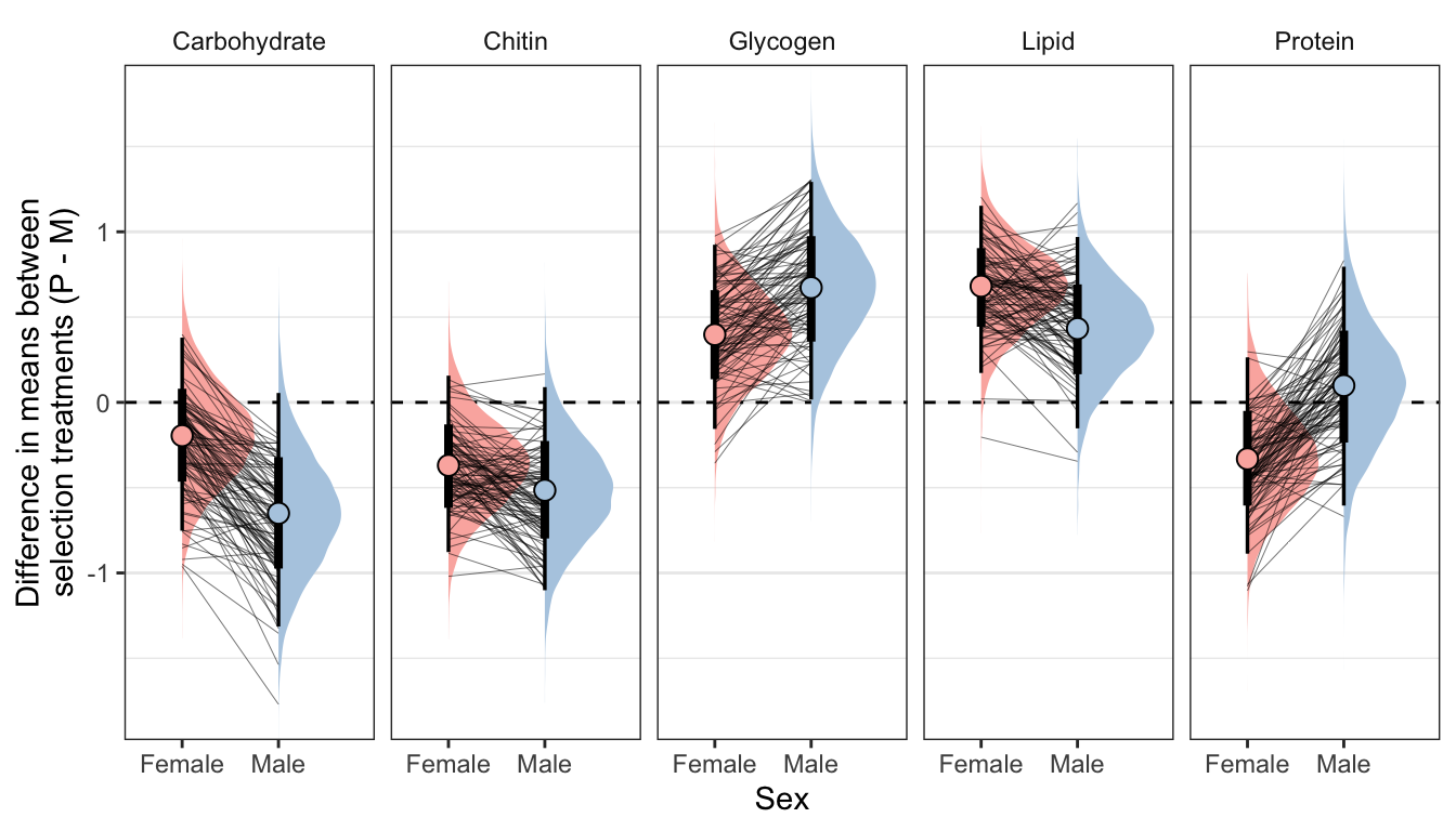
Controlling for differences in dry weight between treatments
treat_diff_standard_dryweight %>%
  filter(variable != 'Dryweight') %>%
  ggplot(aes(x = sex, y = `Difference in means (Poly - Mono)`,fill = sex)) +
  geom_hline(yintercept = 0, linetype = 2) +
  stat_halfeye() +
  geom_line(data = treat_diff_standard_dryweight %>%
              filter(draw %in% sampled_draws) %>%
              filter(variable != 'Dryweight'),
            alpha = 0.8, size = 0.12, colour = "black", aes(group = draw)) +
  geom_point(data = summary_dat1, pch = 21, colour = "black", size = 3.1) +
  scale_fill_brewer(palette = 'Pastel1', direction = 1, name = "") +
  scale_colour_brewer(palette = 'Pastel1', direction = 1, name = "") +
  facet_wrap( ~ variable,  nrow = 1) +
  theme_bw() +
  theme(legend.position = 'none',
        strip.background = element_blank(),
        panel.grid.major.x = element_blank()) +
  coord_cartesian(ylim = ylims) +
  ylab("Difference in means between\nselection treatments (P - M)") + xlab("Sex")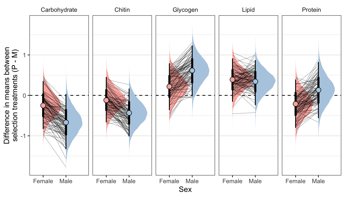
Table
Controlling for differences in dry weight between treatments
summary_dat1 %>%
  kable(digits = 3) %>%
kable_styling(full_width = FALSE)| variable | sex | Difference in means (Poly - Mono) | Lower 95% CI | Upper 95% CI | p | |
|---|---|---|---|---|---|---|
| Carbohydrate | Female | -0.250 | -0.834 | 0.353 | 0.205 | |
| Carbohydrate | Male | -0.668 | -1.326 | 0.036 | 0.031 | * |
| Chitin | Female | -0.119 | -0.667 | 0.456 | 0.336 | |
| Chitin | Male | -0.434 | -1.014 | 0.169 | 0.078 | |
| Glycogen | Female | 0.220 | -0.366 | 0.795 | 0.224 | |
| Glycogen | Male | 0.616 | -0.024 | 1.233 | 0.031 | * |
| Lipid | Female | 0.390 | -0.157 | 0.916 | 0.074 | |
| Lipid | Male | 0.342 | -0.241 | 0.872 | 0.111 | |
| Protein | Female | -0.211 | -0.801 | 0.394 | 0.246 | |
| Protein | Male | 0.132 | -0.562 | 0.826 | 0.347 |
Not controlling for differences in dry weight between treatments
summary_dat2 %>%
  kable(digits = 3) %>%
kable_styling(full_width = FALSE)| variable | sex | Difference in means (Poly - Mono) | Lower 95% CI | Upper 95% CI | p | |
|---|---|---|---|---|---|---|
| Carbohydrate | Female | -0.195 | -0.752 | 0.380 | 0.247 | |
| Carbohydrate | Male | -0.650 | -1.314 | 0.055 | 0.034 | * |
| Chitin | Female | -0.369 | -0.878 | 0.157 | 0.078 | |
| Chitin | Male | -0.515 | -1.101 | 0.089 | 0.047 | * |
| Glycogen | Female | 0.397 | -0.156 | 0.924 | 0.077 | |
| Glycogen | Male | 0.673 | 0.017 | 1.293 | 0.022 | * |
| Lipid | Female | 0.681 | 0.172 | 1.153 | 0.006 | * |
| Lipid | Male | 0.433 | -0.152 | 0.969 | 0.066 | |
| Protein | Female | -0.331 | -0.887 | 0.264 | 0.132 | |
| Protein | Male | 0.099 | -0.605 | 0.795 | 0.386 |
Posterior difference in treatment effect size between sexes
This section essentially examines the treatment \(\times\) sex interaction term, by calculating the difference in the effect size of the P/M treatment between sexes, for each of the five metabolites. We find no strong evidence for a treatment \(\times\) sex interaction, i.e. the treatment effects did not differ detectably between sexes.
Figure
Not controlling for differences in dry weight between treatments
treatsex_interaction_data1 <- treat_diff_actual_dryweight %>%
  select(draw, variable, sex, d =  `Difference in means (Poly - Mono)`) %>%
  arrange(draw, variable, sex) %>%
  group_by(draw, variable) %>%
  summarise(`Difference in effect size between sexes (male - female)` = d[2] - d[1],
            .groups = "drop") # males - females


treatsex_interaction_data1 %>%
  filter(variable != 'Dryweight') %>%
  ggplot(aes(x = `Difference in effect size between sexes (male - female)`, y = 1, fill = stat(x < 0))) +
  geom_vline(xintercept = 0, linetype = 2) +
  stat_halfeyeh() +
  facet_wrap( ~ variable) +
  scale_fill_brewer(palette = 'Pastel2', direction = 1, name = "") +
  theme_bw() +
  theme(legend.position = 'none',
        strip.background = element_blank()) +
  ylab("Posterior density")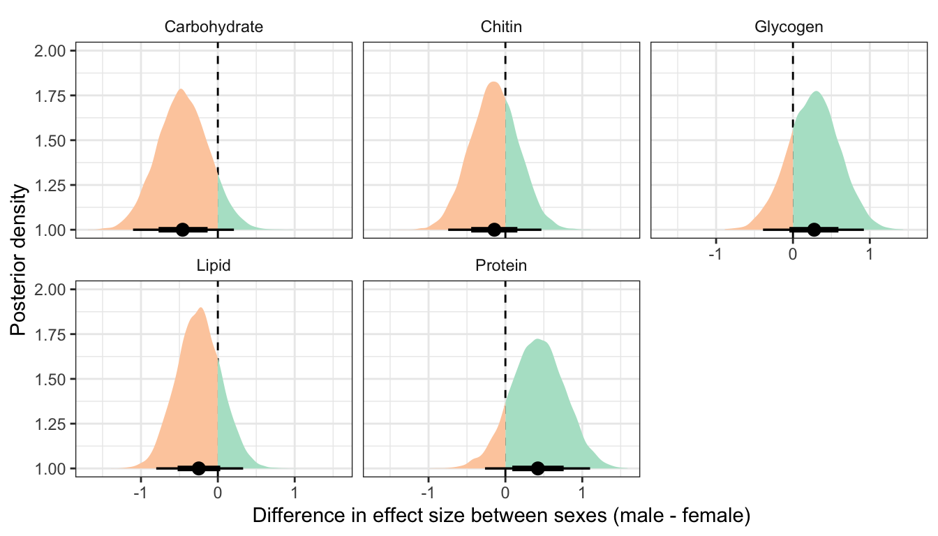
Controlling for differences in dry weight between treatments
treatsex_interaction_data2 <- treat_diff_standard_dryweight %>%
  select(draw, variable, sex, d =  `Difference in means (Poly - Mono)`) %>%
  arrange(draw, variable, sex) %>%
  group_by(draw, variable) %>%
  summarise(`Difference in effect size between sexes (male - female)` = d[2] - d[1],
            .groups = "drop") # males - females

treatsex_interaction_data2 %>%
  filter(variable != 'Dryweight') %>%
  ggplot(aes(x = `Difference in effect size between sexes (male - female)`, y = 1, fill = stat(x < 0))) +
  geom_vline(xintercept = 0, linetype = 2) +
  stat_halfeyeh() +
  facet_wrap( ~ variable) +
  scale_fill_brewer(palette = 'Pastel2', direction = 1, name = "") +
  theme_bw() +
  theme(legend.position = 'none',
        strip.background = element_blank()) +
  ylab("Posterior density")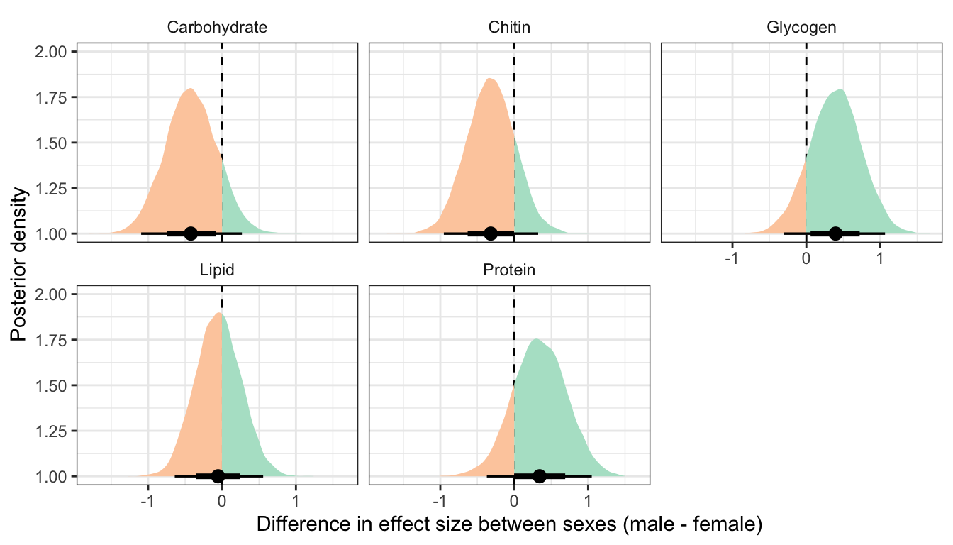
| Version | Author | Date |
|---|---|---|
| f7c88a2 | lukeholman | 2020-12-10 |
Table
Not controlling for differences in dry weight between treatments
treatsex_interaction_data1 %>%
  filter(variable != 'Dryweight') %>%
  rename(x = `Difference in effect size between sexes (male - female)`) %>%
  group_by(variable)  %>%
  summarise(`Difference in effect size between sexes (male - female)` = median(x),
            `Lower 95% CI` = quantile(x, probs = 0.025),
            `Upper 95% CI` = quantile(x, probs = 0.975),
            p = 1 - as.numeric(bayestestR::p_direction(x)),
            ` ` = ifelse(p < 0.05, "\\*", ""),
            .groups = "drop") %>%
  kable(digits=3) %>%
kable_styling(full_width = FALSE)| variable | Difference in effect size between sexes (male - female) | Lower 95% CI | Upper 95% CI | p | |
|---|---|---|---|---|---|
| Carbohydrate | -0.458 | -1.103 | 0.209 | 0.089 | |
| Chitin | -0.143 | -0.744 | 0.469 | 0.326 | |
| Glycogen | 0.276 | -0.390 | 0.922 | 0.208 | |
| Lipid | -0.248 | -0.802 | 0.329 | 0.199 | |
| Protein | 0.423 | -0.265 | 1.102 | 0.113 |
Controlling for differences in dry weight between treatments
treatsex_interaction_data2 %>%
  filter(variable != 'Dryweight') %>%
  rename(x = `Difference in effect size between sexes (male - female)`) %>%
  group_by(variable)  %>%
  summarise(`Difference in effect size between sexes (male - female)` = median(x),
            `Lower 95% CI` = quantile(x, probs = 0.025),
            `Upper 95% CI` = quantile(x, probs = 0.975),
            p = 1 - as.numeric(bayestestR::p_direction(x)),
            ` ` = ifelse(p < 0.05, "\\*", ""),
            .groups = "drop") %>%
  kable(digits=3) %>%
kable_styling(full_width = FALSE)| variable | Difference in effect size between sexes (male - female) | Lower 95% CI | Upper 95% CI | p | |
|---|---|---|---|---|---|
| Carbohydrate | -0.422 | -1.095 | 0.269 | 0.119 | |
| Chitin | -0.317 | -0.953 | 0.324 | 0.168 | |
| Glycogen | 0.397 | -0.305 | 1.065 | 0.134 | |
| Lipid | -0.054 | -0.640 | 0.557 | 0.431 | |
| Protein | 0.344 | -0.371 | 1.050 | 0.171 |
sessionInfo()R version 4.0.3 (2020-10-10) Platform: x86_64-apple-darwin17.0 (64-bit) Running under: macOS Catalina 10.15.4 Matrix products: default BLAS: /Library/Frameworks/R.framework/Versions/4.0/Resources/lib/libRblas.dylib LAPACK: /Library/Frameworks/R.framework/Versions/4.0/Resources/lib/libRlapack.dylib locale: [1] en_AU.UTF-8/en_AU.UTF-8/en_AU.UTF-8/C/en_AU.UTF-8/en_AU.UTF-8 attached base packages: [1] stats graphics grDevices utils datasets methods base other attached packages: [1] knitrhooks_0.0.4 knitr_1.30 kableExtra_1.1.0 DT_0.13 tidybayes_2.0.3 brms_2.14.4 Rcpp_1.0.4.6 ggridges_0.5.2 gridExtra_2.3 [10] GGally_1.5.0 forcats_0.5.0 stringr_1.4.0 dplyr_1.0.0 purrr_0.3.4 readr_1.3.1 tidyr_1.1.0 tibble_3.0.1 ggplot2_3.3.2 [19] tidyverse_1.3.0 workflowr_1.6.2 loaded via a namespace (and not attached): [1] readxl_1.3.1 backports_1.1.7 plyr_1.8.6 igraph_1.2.5 svUnit_1.0.3 splines_4.0.3 crosstalk_1.1.0.1 [8] TH.data_1.0-10 rstantools_2.1.1 inline_0.3.15 digest_0.6.25 htmltools_0.5.0 rsconnect_0.8.16 fansi_0.4.1 [15] magrittr_2.0.1 modelr_0.1.8 RcppParallel_5.0.1 matrixStats_0.56.0 xts_0.12-0 sandwich_2.5-1 prettyunits_1.1.1 [22] colorspace_1.4-1 blob_1.2.1 rvest_0.3.5 haven_2.3.1 xfun_0.19 callr_3.4.3 crayon_1.3.4 [29] jsonlite_1.7.0 lme4_1.1-23 survival_3.2-7 zoo_1.8-8 glue_1.4.2 gtable_0.3.0 emmeans_1.4.7 [36] webshot_0.5.2 V8_3.4.0 pkgbuild_1.0.8 rstan_2.21.2 abind_1.4-5 scales_1.1.1 mvtnorm_1.1-0 [43] DBI_1.1.0 miniUI_0.1.1.1 viridisLite_0.3.0 xtable_1.8-4 stats4_4.0.3 StanHeaders_2.21.0-3 htmlwidgets_1.5.1 [50] httr_1.4.1 DiagrammeR_1.0.6.1 threejs_0.3.3 arrayhelpers_1.1-0 RColorBrewer_1.1-2 ellipsis_0.3.1 farver_2.0.3 [57] pkgconfig_2.0.3 reshape_0.8.8 loo_2.3.1 dbplyr_1.4.4 labeling_0.3 tidyselect_1.1.0 rlang_0.4.6 [64] reshape2_1.4.4 later_1.0.0 visNetwork_2.0.9 munsell_0.5.0 cellranger_1.1.0 tools_4.0.3 cli_2.0.2 [71] generics_0.0.2 broom_0.5.6 evaluate_0.14 fastmap_1.0.1 yaml_2.2.1 processx_3.4.2 fs_1.4.1 [78] nlme_3.1-149 whisker_0.4 mime_0.9 projpred_2.0.2 xml2_1.3.2 compiler_4.0.3 bayesplot_1.7.2 [85] shinythemes_1.1.2 rstudioapi_0.11 gamm4_0.2-6 curl_4.3 reprex_0.3.0 statmod_1.4.34 stringi_1.5.3 [92] highr_0.8 ps_1.3.3 Brobdingnag_1.2-6 lattice_0.20-41 Matrix_1.2-18 nloptr_1.2.2.1 markdown_1.1 [99] shinyjs_1.1 vctrs_0.3.0 pillar_1.4.4 lifecycle_0.2.0 bridgesampling_1.0-0 estimability_1.3 insight_0.8.4 [106] httpuv_1.5.3.1 R6_2.4.1 promises_1.1.0 codetools_0.2-16 boot_1.3-25 colourpicker_1.0 MASS_7.3-53 [113] gtools_3.8.2 assertthat_0.2.1 rprojroot_1.3-2 withr_2.2.0 shinystan_2.5.0 multcomp_1.4-13 bayestestR_0.6.0 [120] mgcv_1.8-33 parallel_4.0.3 hms_0.5.3 grid_4.0.3 coda_0.19-3 minqa_1.2.4 rmarkdown_2.5 [127] git2r_0.27.1 shiny_1.4.0.2 lubridate_1.7.8 base64enc_0.1-3 dygraphs_1.1.1.6