Analysis of Experiment 1
Last updated: 2020-04-21
Checks: 7 0
Knit directory: social_immunity/
This reproducible R Markdown analysis was created with workflowr (version 1.6.0). The Checks tab describes the reproducibility checks that were applied when the results were created. The Past versions tab lists the development history.
Great! Since the R Markdown file has been committed to the Git repository, you know the exact version of the code that produced these results.
Great job! The global environment was empty. Objects defined in the global environment can affect the analysis in your R Markdown file in unknown ways. For reproduciblity it’s best to always run the code in an empty environment.
The command set.seed(20191017) was run prior to running the code in the R Markdown file. Setting a seed ensures that any results that rely on randomness, e.g. subsampling or permutations, are reproducible.
Great job! Recording the operating system, R version, and package versions is critical for reproducibility.
Nice! There were no cached chunks for this analysis, so you can be confident that you successfully produced the results during this run.
Great job! Using relative paths to the files within your workflowr project makes it easier to run your code on other machines.
These are the previous versions of the R Markdown and HTML files. If you’ve configured a remote Git repository (see ?wflow_git_remote), click on the hyperlinks in the table below to view them.
| File | Version | Author | Date | Message |
|---|---|---|---|---|
| Rmd | 1ce9e19 | lukeholman | 2020-04-21 | First commit 2020 |
| html | 1ce9e19 | lukeholman | 2020-04-21 | First commit 2020 |
| Rmd | aae65cf | lukeholman | 2019-10-17 | First commit |
| html | aae65cf | lukeholman | 2019-10-17 | First commit |
Load data and R packages
# All but 1 of these packages can be easily installed from CRAN.
# However it was harder to install the showtext package. On Mac, I did this:
# installed 'homebrew' using Terminal: ruby -e "$(curl -fsSL https://raw.githubusercontent.com/Homebrew/install/master/install)"
# installed 'libpng' using Terminal: brew install libpng
# installed 'showtext' in R using: devtools::install_github("yixuan/showtext")
library(showtext)

library(brms)
library(bayesplot)
library(tidyverse)
library(gridExtra)
library(kableExtra)
library(bayestestR)
library(tidybayes)
library(cowplot)
source("code/helper_functions.R")

# set up nice font for figure
nice_font <- "PT Serif"
font_add_google(name = nice_font, family = nice_font, regular.wt = 400, bold.wt = 700)
showtext_auto()

exp1_treatments <- c("Intact control", "Ringers", "Heat-treated LPS", "LPS")

durations <- read_csv("data/data_collection_sheets/experiment_durations.csv") %>%
  filter(experiment == 1) %>% select(-experiment)

outcome_tally <- read_csv(file = "data/clean_data/experiment_1_outcome_tally.csv") %>%
  mutate(outcome = replace(outcome, outcome == "Left of own volition", "Left voluntarily")) %>%
  mutate(outcome   = factor(outcome, levels = c("Stayed inside the hive", "Left voluntarily", "Forced out")),
         treatment = factor(treatment, levels = exp1_treatments))

# Re-formatted version of the same data, where each row is an individual bee. We need this format to run the brms model.
data_for_categorical_model <- outcome_tally %>%
  mutate(id = 1:n()) %>%
  split(.$id) %>%
  map(function(x){
    if(x$n[1] == 0) return(NULL)
    data.frame(
      treatment = x$treatment[1],
      hive = x$hive[1],
      colour = x$colour[1],
      outcome = rep(x$outcome[1], x$n))
  }) %>% do.call("rbind", .) %>% as_tibble() %>%
  arrange(hive, treatment) %>%
  mutate(outcome_numeric = as.numeric(outcome),
         hive = as.character(hive),
         treatment = factor(treatment, levels = exp1_treatments)) %>%
  left_join(durations, by = "hive") %>%
  mutate(hive = C(factor(hive), sum)) # use sum coding for the factor levels of "hive"
Inspect the raw data
Sample sizes by treatment
data_for_categorical_model %>%
  group_by(treatment) %>%
  summarise(n = n()) %>%
kable() %>% kable_styling(full_width = FALSE)| treatment | n |
|---|---|
| Intact control | 321 |
| Ringers | 153 |
| Heat-treated LPS | 186 |
| LPS | 182 |
Sample sizes by treatment and hive
data_for_categorical_model %>%
  group_by(hive, treatment) %>%
  summarise(n = n()) %>%
kable() %>% kable_styling(full_width = FALSE)| hive | treatment | n |
|---|---|---|
| Garden | Intact control | 77 |
| Garden | Ringers | 41 |
| Garden | Heat-treated LPS | 34 |
| Garden | LPS | 37 |
| SkyLab | Intact control | 105 |
| SkyLab | Heat-treated LPS | 58 |
| SkyLab | LPS | 43 |
| Zoology | Intact control | 106 |
| Zoology | Ringers | 80 |
| Zoology | Heat-treated LPS | 67 |
| Zoology | LPS | 67 |
| Zoology_2 | Intact control | 33 |
| Zoology_2 | Ringers | 32 |
| Zoology_2 | Heat-treated LPS | 27 |
| Zoology_2 | LPS | 35 |
Inspect the results
outcome_tally %>%
  select(-colour) %>%
  kable(digits = 3) %>% kable_styling(full_width = FALSE) %>%
scroll_box(height = "380px")| hive | treatment | outcome | n |
|---|---|---|---|
| Garden | Heat-treated LPS | Stayed inside the hive | 34 |
| Garden | Heat-treated LPS | Left voluntarily | 0 |
| Garden | Heat-treated LPS | Forced out | 0 |
| Garden | Intact control | Stayed inside the hive | 75 |
| Garden | Intact control | Left voluntarily | 0 |
| Garden | Intact control | Forced out | 2 |
| Garden | LPS | Stayed inside the hive | 37 |
| Garden | LPS | Left voluntarily | 0 |
| Garden | LPS | Forced out | 0 |
| Garden | Ringers | Stayed inside the hive | 41 |
| Garden | Ringers | Left voluntarily | 0 |
| Garden | Ringers | Forced out | 0 |
| SkyLab | Heat-treated LPS | Stayed inside the hive | 47 |
| SkyLab | Heat-treated LPS | Left voluntarily | 6 |
| SkyLab | Heat-treated LPS | Forced out | 5 |
| SkyLab | Intact control | Stayed inside the hive | 102 |
| SkyLab | Intact control | Left voluntarily | 3 |
| SkyLab | Intact control | Forced out | 0 |
| SkyLab | LPS | Stayed inside the hive | 35 |
| SkyLab | LPS | Left voluntarily | 6 |
| SkyLab | LPS | Forced out | 2 |
| Zoology | Heat-treated LPS | Stayed inside the hive | 59 |
| Zoology | Heat-treated LPS | Left voluntarily | 1 |
| Zoology | Heat-treated LPS | Forced out | 7 |
| Zoology | Intact control | Stayed inside the hive | 105 |
| Zoology | Intact control | Left voluntarily | 0 |
| Zoology | Intact control | Forced out | 1 |
| Zoology | LPS | Stayed inside the hive | 60 |
| Zoology | LPS | Left voluntarily | 2 |
| Zoology | LPS | Forced out | 5 |
| Zoology | Ringers | Stayed inside the hive | 74 |
| Zoology | Ringers | Left voluntarily | 1 |
| Zoology | Ringers | Forced out | 5 |
| Zoology_2 | Heat-treated LPS | Stayed inside the hive | 16 |
| Zoology_2 | Heat-treated LPS | Left voluntarily | 1 |
| Zoology_2 | Heat-treated LPS | Forced out | 10 |
| Zoology_2 | Intact control | Stayed inside the hive | 24 |
| Zoology_2 | Intact control | Left voluntarily | 1 |
| Zoology_2 | Intact control | Forced out | 8 |
| Zoology_2 | LPS | Stayed inside the hive | 21 |
| Zoology_2 | LPS | Left voluntarily | 2 |
| Zoology_2 | LPS | Forced out | 12 |
| Zoology_2 | Ringers | Stayed inside the hive | 23 |
| Zoology_2 | Ringers | Left voluntarily | 1 |
| Zoology_2 | Ringers | Forced out | 8 |
Raw results as a bar chart
all_hives <- outcome_tally %>%
  group_by(treatment, outcome) %>%
  summarise(n = sum(n)) %>%
  ungroup() %>% mutate(hive = "All hives")

outcome_tally %>%
  group_by(treatment, hive, outcome, .drop = FALSE) %>%
  summarise(n = sum(n)) %>%
  ungroup() %>%
  mutate(hive = paste(hive, "hive")) %>%
  full_join(all_hives, by = c("treatment", "hive", "outcome", "n")) %>%
  split(paste(.$treatment, .$hive)) %>%
  map(~ .x %>% mutate(percent = 100 * n / sum(n))) %>%
  bind_rows()
# A tibble: 57 x 5
treatment hive outcome n percent
<fct> <chr> <fct> <dbl> <dbl>
1 Heat-treated LPS All hives Stayed inside the hive 156 83.9
2 Heat-treated LPS All hives Left voluntarily 8 4.30
3 Heat-treated LPS All hives Forced out 22 11.8
4 Heat-treated LPS Garden hive Stayed inside the hive 34 100
5 Heat-treated LPS Garden hive Left voluntarily 0 0
6 Heat-treated LPS Garden hive Forced out 0 0
7 Heat-treated LPS SkyLab hive Stayed inside the hive 47 81.0
8 Heat-treated LPS SkyLab hive Left voluntarily 6 10.3
9 Heat-treated LPS SkyLab hive Forced out 5 8.62
10 Heat-treated LPS Zoology hive Stayed inside the hive 59 88.1
# … with 47 more rowspd <- position_dodge(.3)
outcome_tally %>%
group_by(treatment, outcome) %>%
summarise(n = sum(n)) %>% mutate() %>%
group_by(treatment) %>%
mutate(total_n = sum(n),
percent = 100 * n / sum(n),
SE = sqrt(total_n * (percent/100) * (1-(percent/100)))) %>%
ungroup() %>%
mutate(lowerCI = map_dbl(1:n(), ~ 100 * binom.test(n[.x], total_n[.x])$conf.int[1]),
upperCI = map_dbl(1:n(), ~ 100 * binom.test(n[.x], total_n[.x])$conf.int[2])) %>%
filter(outcome != "Stayed inside the hive") %>%
ggplot(aes(treatment, percent, fill = outcome)) +
geom_errorbar(aes(ymin=lowerCI, ymax=upperCI), position = pd, width = 0) +
geom_point(stat = "identity", position = pd, colour = "grey15", pch = 21, size = 4) +
scale_fill_brewer(palette = "Pastel1", name = "Outcome", direction = -1) +
xlab("Treatment") + ylab("% bees (+95% CIs)") +
theme(legend.position = "top") +
coord_flip()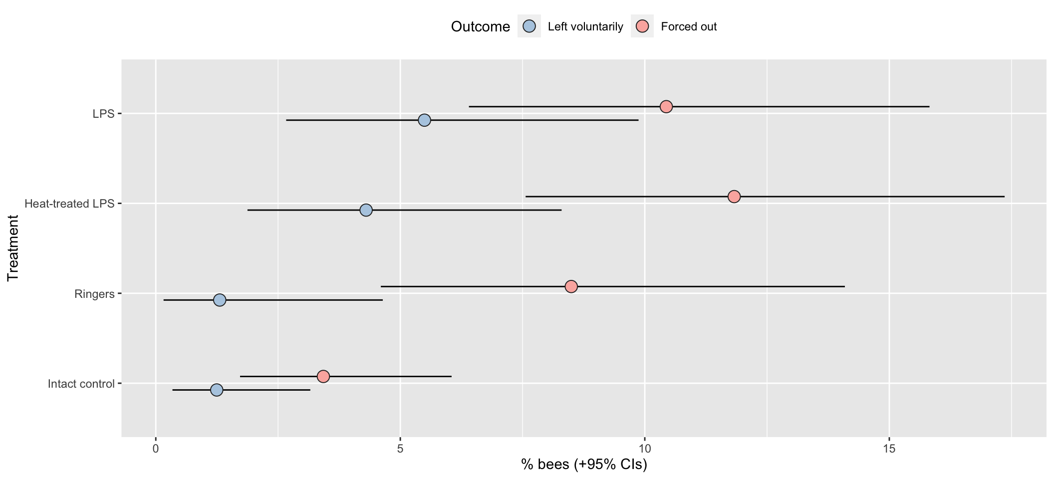
| Version | Author | Date |
|---|---|---|
| 1ce9e19 | lukeholman | 2020-04-21 |
Multinomial model of outcome
Run the models
Fit a multinomial logisitic model, with 3 possible outcomes describing what happened to each bee introduced to the hive: stayed inside, left of its own volition, or forced out by the other workers. To assess the effects of our predictor variables, we compare 5 models with different fixed factors, ranking them by posterior model probability.
if(!file.exists("output/exp1_model.rds")){

  exp1_model_v1 <- brm(
    outcome_numeric ~ treatment * hive + observation_time_minutes,
    data = data_for_categorical_model,
    prior = c(set_prior("normal(0, 3)", class = "b", dpar = "mu2"),
              set_prior("normal(0, 3)", class = "b", dpar = "mu3")),
    family = "categorical", save_all_pars = TRUE, sample_prior = TRUE,
    chains = 4, cores = 1, iter = 5000, seed = 1)

  exp1_model_v2 <- brm(
    outcome_numeric ~ treatment + hive + observation_time_minutes,
    data = data_for_categorical_model,
    prior = c(set_prior("normal(0, 3)", class = "b", dpar = "mu2"),
              set_prior("normal(0, 3)", class = "b", dpar = "mu3")),
    family = "categorical", save_all_pars = TRUE, sample_prior = TRUE,
    chains = 4, cores = 1, iter = 5000, seed = 1)

  exp1_model_v3 <- brm(
    outcome_numeric ~ hive + observation_time_minutes,
    data = data_for_categorical_model,
    prior = c(set_prior("normal(0, 3)", class = "b", dpar = "mu2"),
              set_prior("normal(0, 3)", class = "b", dpar = "mu3")),
    family = "categorical",  save_all_pars = TRUE, sample_prior = TRUE,
    chains = 4, cores = 1, iter = 5000, seed = 1)

  posterior_model_probabilities <- tibble(
    Model = c("treatment * hive + observation_time_minutes",
              "treatment + hive + observation_time_minutes",
              "hive + observation_time_minutes"),
    post_prob = as.numeric(post_prob(exp1_model_v1,
                                     exp1_model_v2,
                                     exp1_model_v3))) %>%
    arrange(-post_prob)

  saveRDS(exp1_model_v2, "output/exp1_model.rds") # save the top model, treatment + hive
  saveRDS(posterior_model_probabilities, "output/exp1_post_prob.rds")
}

exp1_model <- readRDS("output/exp1_model.rds")
posterior_model_probabilities <- readRDS("output/exp1_post_prob.rds")
Fixed effects from the full model
The code chunk below wrangles the raw output of the summary() functions for brms models into a more readable table of results, and also adds ‘Bayesian p-values’ (i.e. the posterior probability that the true effect size has the same sign as the reported effect).
tableS1 <- get_fixed_effects_with_p_values(exp1_model) %>%
  mutate(mu = map_chr(str_extract_all(Parameter, "mu[:digit:]"), ~ .x[1]),
         Parameter = str_remove_all(Parameter, "mu[:digit:]_"),
         Parameter = str_replace_all(Parameter, "treatment", "Treatment: "),
         Parameter = str_replace_all(Parameter, "HeatMtreatedLPS", "Heat-treated LPS"),
         Parameter = str_replace_all(Parameter, "observation_time_minutes", "Observation duration (minutes)")) %>%
  arrange(mu) %>%
  select(-mu, -Rhat, -Bulk_ESS, -Tail_ESS)

names(tableS1)[3:5] <- c("Est. Error", "Lower 95% CI", "Upper 95% CI")

saveRDS(tableS1, file = "figures/tableS1.rds")

tableS1 %>%
  kable(digits = 3) %>%
  kable_styling(full_width = FALSE) %>%
  pack_rows("% bees leaving voluntarily", 1, 8) %>%
pack_rows("% bees forced out", 9, 16)| Parameter | Estimate | Est. Error | Lower 95% CI | Upper 95% CI | p | |
|---|---|---|---|---|---|---|
| % bees leaving voluntarily | ||||||
| Intercept | -14.866 | 9.431 | -35.346 | 2.072 | 0.045 | * |
| Treatment: Ringers | 0.658 | 0.970 | -1.395 | 2.433 | 0.232 | |
| Treatment: Heat-treated LPS | 1.298 | 0.612 | 0.126 | 2.530 | 0.015 | * |
| Treatment: LPS | 1.681 | 0.602 | 0.532 | 2.902 | 0.002 | ** |
| hive1 | -1.514 | 2.617 | -6.596 | 3.576 | 0.281 | |
| hive2 | 3.127 | 1.480 | 0.836 | 6.624 | 0.001 | ** |
| hive3 | -1.520 | 1.602 | -4.785 | 1.564 | 0.172 | |
| Observation duration (minutes) | 0.091 | 0.090 | -0.073 | 0.284 | 0.148 | |
| % bees forced out | ||||||
| Intercept | -7.403 | 6.705 | -20.821 | 5.738 | 0.134 | |
| Treatment: Ringers | 0.552 | 0.453 | -0.341 | 1.445 | 0.114 | |
| Treatment: Heat-treated LPS | 1.298 | 0.406 | 0.520 | 2.097 | 0.000 | *** |
| Treatment: LPS | 0.965 | 0.419 | 0.161 | 1.797 | 0.011 | * |
| hive1 | -0.394 | 2.523 | -5.315 | 4.675 | 0.437 | |
| hive2 | -0.115 | 0.654 | -1.392 | 1.160 | 0.431 | |
| hive3 | -0.762 | 1.518 | -3.826 | 2.200 | 0.309 | |
| Observation duration (minutes) | 0.038 | 0.068 | -0.095 | 0.176 | 0.288 | |
Table S1: Table summarising the posterior estimates of each fixed effect in the best-fitting model of Experiment 1. This was a multinomial model with three possible outcomes (stay inside, leave voluntarily, be forced out), and so there are two parameter estimates for the intercept and for each predictor in the model. ‘Treatment’ is a fixed factor with four levels, and the effects shown here are expressed relative to the ‘Intact control’ group. ‘Hive’ was also a fixed factor with four levels; unlike for treatment, we modelled hive using deviation coding, such that the intercept term represents the mean across all hives (in the intact control treatment), and the three hive terms represent the deviation from this mean for three of the four hives. Lastly, observation duration was a continuous variable expressed to the nearest minute. The \(p\) column gives the posterior probability that the true effect size is opposite in sign to what is reported in the Estimate column, similarly to a p-value.
Plotting estimates from the model
Derive prediction from the posterior
new <- expand.grid(treatment = levels(data_for_categorical_model$treatment),
                   hive = NA,
                   observation_time_minutes = 120)

preds <- fitted(exp1_model, newdata = new, summary = FALSE)
dimnames(preds) <- list(NULL, new[,1], NULL)

plotting_data <- rbind(
  as.data.frame(preds[,, 1]) %>% mutate(outcome = "Stayed inside the hive", posterior_sample = 1:n()),
  as.data.frame(preds[,, 2]) %>% mutate(outcome = "Left voluntarily", posterior_sample = 1:n()),
  as.data.frame(preds[,, 3]) %>% mutate(outcome = "Forced out", posterior_sample = 1:n())) %>%
  gather(treatment, prop, `Intact control`, Ringers, `Heat-treated LPS`, LPS) %>%
  mutate(outcome = factor(outcome, c("Stayed inside the hive", "Left voluntarily", "Forced out"))) %>%
  as_tibble() %>% arrange(treatment, outcome)

stats_data <- plotting_data
plotting_data$treatment <- factor(plotting_data$treatment, c("Intact control", "Ringers", "Heat-treated LPS", "LPS"))
Make Figure 1
cols <- c("#34558b", "#4ec5a5", "#ffaf12")

dot_plot <- plotting_data %>%
  mutate(outcome = str_replace_all(outcome, "Stayed inside the hive", "Stayed inside"),
         outcome = factor(outcome, c("Stayed inside", "Left voluntarily", "Forced out"))) %>%
  ggplot(aes(100 * prop, treatment)) +
  stat_dotsh(quantiles = 100, fill = "grey40", colour = "grey40") + # aes(fill = treatment),
  stat_pointintervalh(aes(colour = outcome, fill = outcome),
                      .width = c(0.5, 0.95),
                      position = position_nudge(y = -0.07),
                      point_colour = "grey26", pch = 21, stroke = 0.4) +
  scale_colour_manual(values = cols) +
  scale_fill_manual(values = cols) +
  facet_wrap( ~ outcome, scales = "free_x") +
  xlab("% bees (posterior estimate)") + ylab("Treatment") +
  theme_bw() +
  coord_cartesian(ylim=c(1.4, 4)) +
  theme(
    text = element_text(family = nice_font),
    strip.background = element_rect(fill = "#eff0f1"),
    panel.grid.major.y = element_blank(),
    legend.position = "none"
  )


get_log_odds <- function(trt1, trt2){ # positive effect = odds of this outcome are higher for trt2 than trt1 (put control as trt1)
  log((trt2 / (1 - trt2) / (trt1 / (1 - trt1))))
}

LOR <- stats_data %>%
  spread(treatment, prop) %>%
  mutate(LOR_intact_Ringers = get_log_odds(`Intact control`, Ringers),
         LOR_intact_heat = get_log_odds(`Intact control`, `Heat-treated LPS`),
         LOR_intact_LPS = get_log_odds(`Intact control`, LPS),
         LOR_Ringers_heat = get_log_odds(Ringers, `Heat-treated LPS`),
         LOR_Ringers_LPS = get_log_odds(Ringers, LPS),
         LOR_heat_LPS = get_log_odds(`Heat-treated LPS`, LPS)) %>%
  select(posterior_sample, outcome, starts_with("LOR")) %>%
  gather(LOR, comparison, starts_with("LOR")) %>%
  mutate(LOR = str_remove_all(LOR, "LOR_"),
         LOR = str_replace_all(LOR, "heat_LPS", "LPS\n(Heat-treated LPS)"),
         LOR = str_replace_all(LOR, "Ringers_LPS", "LPS\n(Ringers)"),
         LOR = str_replace_all(LOR, "Ringers_heat", "Heat-treated LPS\n(Ringers)"),
         LOR = str_replace_all(LOR, "intact_Ringers", "Ringers\n(Intact control)"),
         LOR = str_replace_all(LOR, "intact_heat", "Heat-treated LPS\n(Intact control)"),
         LOR = str_replace_all(LOR, "intact_LPS", "LPS\n(Intact control)"))

levs <- LOR$LOR %>% unique() %>% sort()
LOR$LOR <- factor(LOR$LOR, rev(levs[c(3,5,4,2,1,6)]))

LOR_plot <- LOR %>%
  mutate(outcome = str_replace_all(outcome, "Stayed inside the hive", "Stayed inside"),
         outcome = factor(outcome, levels = rev(c("Forced out", "Left voluntarily", "Stayed inside")))) %>%
  # filter(outcome != "Stayed inside the hive") %>%
  ggplot(aes(comparison, y = LOR, colour = outcome)) +
  geom_vline(xintercept = 0, linetype = 2) +
  geom_vline(xintercept = 0.6931472, linetype = 2, colour = "pink") +
  geom_vline(xintercept = -0.6931472, linetype = 2, colour = "pink") +
  stat_pointintervalh(aes(colour = outcome, fill = outcome),
                      .width = c(0.5, 0.95),
                      position = position_dodge(0.5),
                      point_colour = "grey26", pch = 21, stroke = 0.4) +
  scale_colour_manual(values = cols) +
  scale_fill_manual(values = cols) +
  xlab("Effect size (posterior log odds ratio)") + ylab("Treatment (reference)") +
  theme_bw() +
  theme(
    text = element_text(family = nice_font),
    panel.grid.major.y = element_blank(),
    legend.position = "none"
  )


p <- cowplot::plot_grid(plotlist = list(dot_plot, LOR_plot), labels = c("A", "B"),
                   nrow = 2, align = 'v', axis = 'l', rel_heights = c(1.4, 1))
ggsave(plot = p, filename = "figures/fig1.pdf", height = 7, width = 4.7)
p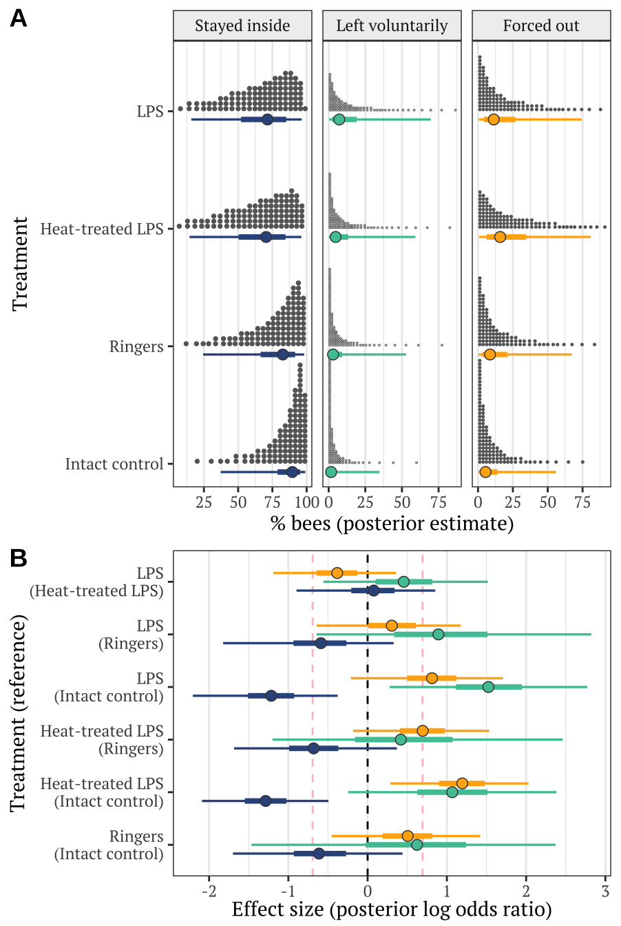
| Version | Author | Date |
|---|---|---|
| 1ce9e19 | lukeholman | 2020-04-21 |
Figure 1: Panel A shows the posterior estimate of the mean % bees staying inside the hive (left), leaving voluntarily (middle), or being forced out (right), in each of the four treatments. The quantile dot plot shows 100 approximately equally likely estimates of the true % bees, and the bars mark the median and the 50% and 95% credible intervals. Panel B gives the posterior estimates of the effect size of each treatment, relative to one of the ‘controls’ (the name of which appears in parentheses), and expressed as a log odds ratio (LOR). Positive LOR indicates that the % bees showing this particular outcome is higher in the treatment than the control, while negative LOR indicates higer % bees in the control. For example, we see that a higher % bees left voluntarily (green) or were forced out (orange) in the LPS treatment relative to the intact control, while the controls were more likely to stay inside the hive (blue). Estimates of LOR for which the 95% credible intervals do not overlap zero are statistically significant in the conventional sense. The dashed red lines indicate LOR = log(\(\pm\) 2), i.e. the point at which the odds are twice as high in one treatment as the other. The model used to derive this figure is described in Tables XX-XX.
Hypothesis testing and effect sizes
This section calculates the posterior difference in treatment group means, in order to perform some null hypothesis testing, calculate effect size, and calculate the 95% credible intervals on the effect size.
We regard both the “Intact control” treatment, and the “Ringers injection” treatment as control groups. The heat-treated LPS group was intended as a control, but post-hoc inspection of the results suggests that the heat-treated LPS had a similar effect on behaviour as did regular LPS (this might explain why heat-treated LPS is very seldom used as a control in insect studies). Therefore, we computed the effect sizes and “Bayesian p-values” (i.e. the fraction of the posterior difference in means that lies on the opposite side of zero from the median) for comparisons between each control and each LPS treatment. We do this three times, once for each of the 3 possible outcomes.
% bees exiting the hive
my_summary <- function(df, columns) {
  lapply(columns, function(x){

    p <- 1 - (df %>% pull(!! x) %>%
                bayestestR::p_direction() %>% as.numeric())

    df %>% pull(!! x) %>% posterior_summary() %>% as_tibble() %>%
      mutate(p=p) %>% mutate(Metric = x) %>% select(Metric, everything()) %>%
      mutate(` ` = ifelse(p < 0.1, "~", ""),
             ` ` = replace(` `, p < 0.05, "\\*"),
             ` ` = replace(` `, p < 0.01, "**"),
             ` ` = replace(` `, p < 0.001, "***"),
             ` ` = replace(` `, p == " ", ""))
  }) %>% do.call("rbind", .)
}


make_stats_table <- function(
  dat, groupA, groupB, comparison,
  metric = "Absolute difference in % bees exiting the hive"){

  output <- dat %>%
    spread(treatment, prop) %>%
    mutate(
      metric_here = 100 * (!! enquo(groupA) - !! enquo(groupB)),
      `Log odds ratio` = get_log_odds(!! enquo(groupB), !! enquo(groupA))) %>%
    my_summary(c("metric_here", "Log odds ratio")) %>%
    mutate(p = c(" ", format(round(p[2], 4), nsmall = 4)),
           ` ` = c(" ", ` `[2]),
           Comparison = comparison) %>%
    select(Comparison, everything()) %>%
    mutate(Metric = replace(Metric, Metric == "metric_here", metric))

  names(output)[names(output) == "metric_here"] <- metric
  output
}

stats_table <- rbind(
  stats_data %>%
    filter(outcome == "Stayed inside the hive") %>%
    make_stats_table(`Intact control`, `Heat-treated LPS`, "Heat-treated LPS (Intact control)"),

  stats_data %>%
    filter(outcome == "Stayed inside the hive") %>%
    make_stats_table(`Ringers`, `Heat-treated LPS`, "Heat-treated LPS (Ringers)"),

  stats_data %>%
    filter(outcome == "Stayed inside the hive") %>%
    make_stats_table(`Intact control`, `LPS`, "LPS (Intact control)"),

  stats_data %>%
    filter(outcome == "Stayed inside the hive") %>%
    make_stats_table(`Ringers`, `LPS`, "LPS (Ringers control)")
) %>% as_tibble()

stats_table[c(2,4,6,8), 1] <- " "

stats_table %>%
  kable(digits = 3) %>% kable_styling(full_width = FALSE) %>%
row_spec(c(0,2,4,6,8), extra_css = "border-bottom: solid;")| Comparison | Metric | Estimate | Est.Error | Q2.5 | Q97.5 | p | |
|---|---|---|---|---|---|---|---|
| Heat-treated LPS (Intact control) | Absolute difference in % bees exiting the hive | 18.252 | 10.719 | 2.128 | 40.405 | ||
| Log odds ratio | 1.286 | 0.405 | 0.495 | 2.091 | 0.0021 | ** | |
| Heat-treated LPS (Ringers) | Absolute difference in % bees exiting the hive | 10.520 | 9.660 | -5.765 | 31.873 | ||
| Log odds ratio | 0.677 | 0.512 | -0.370 | 1.685 | 0.0840 | ~ | |
| LPS (Intact control) | Absolute difference in % bees exiting the hive | 17.269 | 10.862 | 1.887 | 42.029 | ||
| Log odds ratio | 1.233 | 0.458 | 0.377 | 2.205 | 0.0021 | ** | |
| LPS (Ringers control) | Absolute difference in % bees exiting the hive | 9.538 | 9.871 | -5.345 | 33.805 | ||
| Log odds ratio | 0.624 | 0.542 | -0.328 | 1.823 | 0.1047 |
% bees that were forced out
stats_table2 <- rbind(
  stats_data %>%
    filter(outcome == "Forced out") %>%
    make_stats_table(`Intact control`, `Heat-treated LPS`,
                     "Heat-treated LPS (Intact control)",
                     metric = "Absolute difference in % bees that were forced out"),

  stats_data %>%
    filter(outcome == "Forced out") %>%
    make_stats_table(`Ringers`, `Heat-treated LPS`,
                     "Heat-treated LPS (Ringers)",
                     metric = "Absolute difference in % bees that were forced out"),

  stats_data %>%
    filter(outcome == "Forced out") %>%
    make_stats_table(`Intact control`, `LPS`,
                     "LPS (Intact control)",
                     metric = "Absolute difference in % bees that were forced out"),

  stats_data %>%
    filter(outcome == "Forced out") %>%
    make_stats_table(`Ringers`, `LPS`,
                     "LPS (Ringers)",
                     metric = "Absolute difference in % bees that were forced out")
) %>% as_tibble()

stats_table2[c(2,4,6,8), 1] <- " "

stats_table2 %>%
  kable(digits = 3) %>% kable_styling(full_width = FALSE) %>%
row_spec(c(0,2,4,6,8), extra_css = "border-bottom: solid;")| Comparison | Metric | Estimate | Est.Error | Q2.5 | Q97.5 | p | |
|---|---|---|---|---|---|---|---|
| Heat-treated LPS (Intact control) | Absolute difference in % bees that were forced out | -12.381 | 10.494 | -36.953 | -0.321 | ||
| Log odds ratio | -1.185 | 0.445 | -2.031 | -0.285 | 0.0078 | ** | |
| Heat-treated LPS (Ringers) | Absolute difference in % bees that were forced out | -7.884 | 7.865 | -27.155 | 1.338 | ||
| Log odds ratio | -0.689 | 0.438 | -1.534 | 0.183 | 0.0556 | ~ | |
| LPS (Intact control) | Absolute difference in % bees that were forced out | -7.762 | 8.266 | -28.688 | 0.831 | ||
| Log odds ratio | -0.795 | 0.484 | -1.707 | 0.213 | 0.0535 | ~ | |
| LPS (Ringers) | Absolute difference in % bees that were forced out | -3.265 | 6.309 | -19.169 | 7.385 | ||
| Log odds ratio | -0.299 | 0.460 | -1.175 | 0.643 | 0.2446 |
% bees that left voluntarily
stats_table3 <- rbind(
  stats_data %>%
    filter(outcome == "Left voluntarily") %>%
    make_stats_table(`Intact control`, `Heat-treated LPS`,
                     "Heat-treated LPS (Intact control)",
                     metric = "Absolute difference in % bees that left voluntarily"),

  stats_data %>%
    filter(outcome == "Left voluntarily") %>%
    make_stats_table(`Ringers`, `Heat-treated LPS`,
                     "Heat-treated LPS (Ringers control)",
                     metric = "Absolute difference in % bees that left voluntarily"),

  stats_data %>%
    filter(outcome == "Left voluntarily") %>%
    make_stats_table(`Intact control`, `LPS`,
                     "LPS (Intact control)",
                     metric = "Absolute difference in % bees that left voluntarily"),

  stats_data %>%
    filter(outcome == "Left voluntarily") %>%
    make_stats_table(`Ringers`, `LPS`,
                     "LPS (Ringers)",
                     metric = "Absolute difference in % bees that left voluntarily")
) %>% as_tibble()

stats_table3[c(2,4,6,8), 1] <- " "

stats_table3 %>%
  kable(digits = 3) %>% kable_styling(full_width = FALSE) %>%
row_spec(c(0,2,4,6,8), extra_css = "border-bottom: solid;")| Comparison | Metric | Estimate | Est.Error | Q2.5 | Q97.5 | p | |
|---|---|---|---|---|---|---|---|
| Heat-treated LPS (Intact control) | Absolute difference in % bees that left voluntarily | -5.870 | 8.330 | -30.993 | 0.477 | ||
| Log odds ratio | -1.068 | 0.665 | -2.384 | 0.245 | 0.0546 | ~ | |
| Heat-treated LPS (Ringers control) | Absolute difference in % bees that left voluntarily | -2.636 | 8.405 | -25.565 | 11.877 | ||
| Log odds ratio | -0.487 | 0.941 | -2.461 | 1.201 | 0.3086 | ||
| LPS (Intact control) | Absolute difference in % bees that left voluntarily | -9.507 | 11.023 | -40.613 | -0.130 | ||
| Log odds ratio | -1.528 | 0.632 | -2.771 | -0.278 | 0.0091 | ** | |
| LPS (Ringers) | Absolute difference in % bees that left voluntarily | -6.273 | 10.014 | -35.002 | 5.239 | ||
| Log odds ratio | -0.947 | 0.905 | -2.822 | 0.645 | 0.1396 |
sessionInfo()R version 3.6.3 (2020-02-29)
Platform: x86_64-apple-darwin15.6.0 (64-bit)
Running under: macOS Catalina 10.15.4
Matrix products: default
BLAS: /Library/Frameworks/R.framework/Versions/3.6/Resources/lib/libRblas.0.dylib
LAPACK: /Library/Frameworks/R.framework/Versions/3.6/Resources/lib/libRlapack.dylib
locale:
[1] en_AU.UTF-8/en_AU.UTF-8/en_AU.UTF-8/C/en_AU.UTF-8/en_AU.UTF-8
attached base packages:
[1] stats graphics grDevices utils datasets methods base
other attached packages:
[1] cowplot_1.0.0 tidybayes_2.0.1 bayestestR_0.5.1 kableExtra_1.1.0
[5] gridExtra_2.3 forcats_0.5.0 stringr_1.4.0 dplyr_0.8.5
[9] purrr_0.3.3 readr_1.3.1 tidyr_1.0.2 tibble_3.0.0
[13] ggplot2_3.3.0 tidyverse_1.3.0 bayesplot_1.7.1 brms_2.12.0
[17] Rcpp_1.0.3 showtext_0.7-1 showtextdb_2.0 sysfonts_0.8
[21] workflowr_1.6.0
loaded via a namespace (and not attached):
[1] colorspace_1.4-1 ellipsis_0.3.0 ggridges_0.5.2
[4] rsconnect_0.8.16 rprojroot_1.3-2 markdown_1.1
[7] base64enc_0.1-3 fs_1.3.1 rstudioapi_0.11
[10] farver_2.0.3 rstan_2.19.3 svUnit_0.7-12
[13] DT_0.13 fansi_0.4.1 mvtnorm_1.1-0
[16] lubridate_1.7.8 xml2_1.3.1 bridgesampling_1.0-0
[19] knitr_1.28 shinythemes_1.1.2 jsonlite_1.6.1
[22] broom_0.5.4 dbplyr_1.4.2 shiny_1.4.0
[25] compiler_3.6.3 httr_1.4.1 backports_1.1.6
[28] assertthat_0.2.1 Matrix_1.2-18 fastmap_1.0.1
[31] cli_2.0.2 later_1.0.0 htmltools_0.4.0
[34] prettyunits_1.1.1 tools_3.6.3 igraph_1.2.5
[37] coda_0.19-3 gtable_0.3.0 glue_1.4.0
[40] reshape2_1.4.4 cellranger_1.1.0 vctrs_0.2.4
[43] nlme_3.1-147 crosstalk_1.1.0.1 insight_0.8.1
[46] xfun_0.13 ps_1.3.0 rvest_0.3.5
[49] mime_0.9 miniUI_0.1.1.1 lifecycle_0.2.0
[52] gtools_3.8.2 zoo_1.8-7 scales_1.1.0
[55] colourpicker_1.0 hms_0.5.3 promises_1.1.0
[58] Brobdingnag_1.2-6 parallel_3.6.3 inline_0.3.15
[61] RColorBrewer_1.1-2 shinystan_2.5.0 curl_4.3
[64] yaml_2.2.1 loo_2.2.0 StanHeaders_2.19.2
[67] stringi_1.4.6 highr_0.8 dygraphs_1.1.1.6
[70] pkgbuild_1.0.6 rlang_0.4.5 pkgconfig_2.0.3
[73] matrixStats_0.56.0 evaluate_0.14 lattice_0.20-41
[76] labeling_0.3 rstantools_2.0.0 htmlwidgets_1.5.1
[79] processx_3.4.2 tidyselect_1.0.0 plyr_1.8.6
[82] magrittr_1.5 R6_2.4.1 generics_0.0.2
[85] DBI_1.1.0 pillar_1.4.3 haven_2.2.0
[88] whisker_0.4 withr_2.1.2 xts_0.12-0
[91] abind_1.4-5 modelr_0.1.5 crayon_1.3.4
[94] arrayhelpers_1.1-0 utf8_1.1.4 rmarkdown_2.1
[97] grid_3.6.3 readxl_1.3.1 callr_3.4.3
[100] git2r_0.26.1 threejs_0.3.3 reprex_0.3.0
[103] digest_0.6.25 webshot_0.5.2 xtable_1.8-4
[106] httpuv_1.5.2 stats4_3.6.3 munsell_0.5.0
[109] viridisLite_0.3.0 shinyjs_1.1