PS05_Prelim_results
Liam and Charlotte
2026-03-04
Last updated: 2026-03-25
Checks: 7 0
Knit directory: dickinson_power/
This reproducible R Markdown analysis was created with workflowr (version 1.7.2). The Checks tab describes the reproducibility checks that were applied when the results were created. The Past versions tab lists the development history.
Great! Since the R Markdown file has been committed to the Git repository, you know the exact version of the code that produced these results.
Great job! The global environment was empty. Objects defined in the global environment can affect the analysis in your R Markdown file in unknown ways. For reproduciblity it’s best to always run the code in an empty environment.
The command set.seed(20260107) was run prior to running
the code in the R Markdown file. Setting a seed ensures that any results
that rely on randomness, e.g. subsampling or permutations, are
reproducible.
Great job! Recording the operating system, R version, and package versions is critical for reproducibility.
Nice! There were no cached chunks for this analysis, so you can be confident that you successfully produced the results during this run.
Great job! Using relative paths to the files within your workflowr project makes it easier to run your code on other machines.
Great! You are using Git for version control. Tracking code development and connecting the code version to the results is critical for reproducibility.
The results in this page were generated with repository version 474aa52. See the Past versions tab to see a history of the changes made to the R Markdown and HTML files.
Note that you need to be careful to ensure that all relevant files for
the analysis have been committed to Git prior to generating the results
(you can use wflow_publish or
wflow_git_commit). workflowr only checks the R Markdown
file, but you know if there are other scripts or data files that it
depends on. Below is the status of the Git repository when the results
were generated:
Ignored files:
    Ignored:    .DS_Store
    Ignored:    .Rhistory
    Ignored:    .Rproj.user/
    Ignored:    analysis/.DS_Store
    Ignored:    analysis_to-fix/.DS_Store
    Ignored:    data/.DS_Store
    Ignored:    data/FY25 Main Meter Data.xlsx
    Ignored:    data/building_list_FY25_updated.xlsx
    Ignored:    data/graph_data_life_exp.csv
    Ignored:    data/housing_counts.csv
    Ignored:    keys/.DS_Store
    Ignored:    output/annual_kwh.csv
    Ignored:    output/building_check.csv
    Ignored:    output/building_check.xlsx
    Ignored:    output/daily_kwh.csv
    Ignored:    output/kwh_academic_2026-03-16.csv
    Ignored:    output/kwh_academic_2026-03-17.csv
    Ignored:    output/kwh_academic_2026-03-18.csv
    Ignored:    output/kwh_academic_2026-03-22.csv
    Ignored:    output/kwh_academic_2026-03-23.csv
    Ignored:    output/kwh_academic_2026-03-25.csv
    Ignored:    output/kwh_annual.csv
    Ignored:    output/kwh_annual_2026-03-04.csv
    Ignored:    output/kwh_annual_2026-03-12.csv
    Ignored:    output/kwh_annual_2026-03-16.csv
    Ignored:    output/kwh_annual_2026-03-17.csv
    Ignored:    output/kwh_annual_2026-03-18.csv
    Ignored:    output/kwh_annual_2026-03-22.csv
    Ignored:    output/kwh_annual_2026-03-23.csv
    Ignored:    output/kwh_annual_2026-03-25.csv
    Ignored:    output/kwh_annual_20260225.csv
    Ignored:    output/kwh_annual_20260226.csv
    Ignored:    output/kwh_daily.csv
    Ignored:    output/kwh_daily_2026-03-04.csv
    Ignored:    output/kwh_daily_2026-03-12.csv
    Ignored:    output/kwh_daily_2026-03-16.csv
    Ignored:    output/kwh_daily_2026-03-17.csv
    Ignored:    output/kwh_daily_2026-03-18.csv
    Ignored:    output/kwh_daily_2026-03-22.csv
    Ignored:    output/kwh_daily_2026-03-23.csv
    Ignored:    output/kwh_daily_2026-03-25.csv
    Ignored:    output/kwh_daily_20260225.csv
    Ignored:    output/kwh_daily_20260226.csv
    Ignored:    output/kwh_main_annual.csv
    Ignored:    output/kwh_main_daily.csv
Note that any generated files, e.g. HTML, png, CSS, etc., are not included in this status report because it is ok for generated content to have uncommitted changes.
These are the previous versions of the repository in which changes were
made to the R Markdown
(analysis/PS05_prelim_results_Res_Hall_M.Rmd) and HTML
(docs/PS05_prelim_results_Res_Hall_M.html) files. If you’ve
configured a remote Git repository (see ?wflow_git_remote),
click on the hyperlinks in the table below to view the files as they
were in that past version.
| File | Version | Author | Date | Message |
|---|---|---|---|---|
| html | 4ab0c63 | maggiedouglas | 2026-03-23 | Build site. |
| Rmd | 38132bb | maggiedouglas | 2026-03-11 | add student draft results |
| html | 38132bb | maggiedouglas | 2026-03-11 | add student draft results |
Data Preparation
Conversion Factors
dol_per_kWh <- 0.081385
MTCO2_per_kWh <- 0.00030082405
Libraries
library(tidyverse)
library(DT)
Annual Electricity Data
annual_kwh.df<-read.csv('./output/kwh_annual_2026-03-04.csv', strip.white=TRUE) #load data

str(annual_kwh.df) #check data

med_res_annual_kwh<-annual_kwh.df %>% #wrangle for building group annually
  filter(type=="Res Hall - M")


transform_med<-med_res_annual_kwh%>%
  mutate(
    cost=round(kwh_corr*dol_per_kWh, digits=0),
    GHG_emis=round(kwh_corr*MTCO2_per_kWh, digits=0),
    kWh_per_sqft=round(kwh_corr/sqft, digits=1),
    kWh_per_person= round(kwh_corr/occupants, digits=0)
    )

  building_results<-transform_med %>%
    select(NAME, kwh_corr, kWh_per_sqft, cost, GHG_emis, kWh_per_person, meter, days_perc) %>%
  arrange(desc(kwh_corr))
Daily Electricity Data
med_res_daily_kwh <- read.csv("./output/kwh_daily_2026-03-04.csv")
str(med_res_daily_kwh)
med_res_daily_kwh <- med_res_daily_kwh %>%
  filter(type == "Res Hall - M") %>%
  mutate(date = ymd(date),
         month = month(date, label= TRUE),
         day = wday(date, label = TRUE)) %>%
  mutate(kwh_sqft_year = kwh/sqft*365, kwh_person_year = kwh/occupants*365) %>%
  arrange(desc(kwh))
Building Type Summary
Descriptive Table
datatable(building_results,
          filter='top',
          rownames=FALSE,
          colnames = c("Building", "kWh", "kWh per sqft","Cost-$", "CO2e - MT", "kWh per person", "Meter", "Days of data (%)"),
          caption='Table 1. Annual Electricity Use Indicators by Medium Residence Hall in Fiscal Year 2025')
Electrcity Use Over the Year ’
ggplot() +
  annotate("rect", xmin = -Inf, xmax = Inf, ymin = 7.4, ymax = 14.3, color = "lightgray", alpha = 0.3) +
  geom_hline(yintercept = 10.3, linetype = "dashed", color = "white") +
  geom_boxplot(data = med_res_daily_kwh, aes(x = reorder(NAME, kwh_sqft_year, FUN = median), y = kwh_sqft_year, fill = NAME), show.legend = FALSE) +
  coord_flip() +
  labs(
    x = "",
    y = "Electricity Intensity (kWh/sqft/year)",
    title = "Electricity Intensity in Medium Residential Halls \nin the Fiscal Year 2025",
    subtitle = "Buildings ordered by median energy intensity") +
  theme_bw()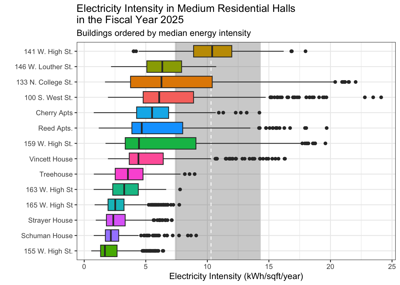
| Version | Author | Date |
|---|---|---|
| 38132bb | maggiedouglas | 2026-03-11 |
Electricity Intensity
ggplot(med_res_daily_kwh , aes(x=month, y=kwh, fill=NAME))+
  geom_bar(position="stack", stat="identity")+
  theme_bw()+
  labs(x="",
       y="Electricity Use (kWh)",
       fill= "Building",
       title= "Monthly Electricity Use by Medium Residence Hall in Fiscal Year 2025")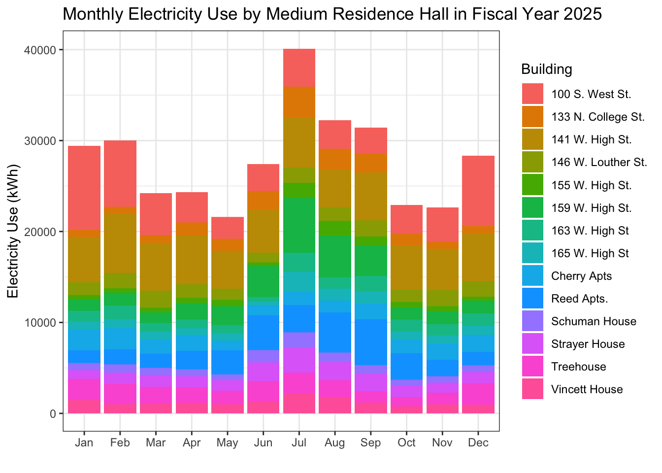
| Version | Author | Date |
|---|---|---|
| 38132bb | maggiedouglas | 2026-03-11 |
Partner Contributions
Charlotte prepared the annual electricity data for this problem set while Liam prepared the daily electricity data. For the building type summary, Charlotte adapted a table she had made last lab to create the summarizing table for annual electricity use indicators by building, Liam created the ranked box plot of daily electricity intensity by building, and Charlotte created the stacked bar graph to show electricity use by month. The data seems to have no issues or problems, all the data is individually metered and clear. There is no missing data. There is occupancy data for all buildings and 100% of the days in the 2025 Fiscal Year were measured.
sessionInfo()R version 4.5.2 (2025-10-31)
Platform: x86_64-apple-darwin20
Running under: macOS Ventura 13.7.8
Matrix products: default
BLAS: /Library/Frameworks/R.framework/Versions/4.5-x86_64/Resources/lib/libRblas.0.dylib
LAPACK: /Library/Frameworks/R.framework/Versions/4.5-x86_64/Resources/lib/libRlapack.dylib; LAPACK version 3.12.1
locale:
[1] en_US.UTF-8/en_US.UTF-8/en_US.UTF-8/C/en_US.UTF-8/en_US.UTF-8
time zone: America/New_York
tzcode source: internal
attached base packages:
[1] stats graphics grDevices utils datasets methods base
other attached packages:
[1] DT_0.34.0 lubridate_1.9.5 forcats_1.0.1 stringr_1.6.0
[5] dplyr_1.2.0 purrr_1.2.1 readr_2.2.0 tidyr_1.3.2
[9] tibble_3.3.1 ggplot2_4.0.2 tidyverse_2.0.0 workflowr_1.7.2
loaded via a namespace (and not attached):
[1] sass_0.4.10 generics_0.1.4 stringi_1.8.7 hms_1.1.4
[5] digest_0.6.39 magrittr_2.0.4 timechange_0.4.0 evaluate_1.0.5
[9] grid_4.5.2 RColorBrewer_1.1-3 fastmap_1.2.0 rprojroot_2.1.1
[13] jsonlite_2.0.0 processx_3.8.6 whisker_0.4.1 ps_1.9.1
[17] promises_1.5.0 httr_1.4.8 crosstalk_1.2.2 scales_1.4.0
[21] jquerylib_0.1.4 cli_3.6.5 rlang_1.1.7 withr_3.0.2
[25] cachem_1.1.0 yaml_2.3.12 otel_0.2.0 tools_4.5.2
[29] tzdb_0.5.0 httpuv_1.6.16 vctrs_0.7.1 R6_2.6.1
[33] lifecycle_1.0.5 git2r_0.36.2 htmlwidgets_1.6.4 fs_1.6.7
[37] pkgconfig_2.0.3 callr_3.7.6 pillar_1.11.1 bslib_0.10.0
[41] later_1.4.8 gtable_0.3.6 glue_1.8.0 Rcpp_1.1.1
[45] xfun_0.56 tidyselect_1.2.1 rstudioapi_0.18.0 knitr_1.51
[49] farver_2.1.2 htmltools_0.5.9 labeling_0.4.3 rmarkdown_2.30
[53] compiler_4.5.2 getPass_0.2-4 S7_0.2.1