E. coli K12 analysis
Last updated: 2022-04-06
Checks: 7 0
Knit directory: rare-mutation-detection/
This reproducible R Markdown analysis was created with workflowr (version 1.6.2). The Checks tab describes the reproducibility checks that were applied when the results were created. The Past versions tab lists the development history.
Great! Since the R Markdown file has been committed to the Git repository, you know the exact version of the code that produced these results.
Great job! The global environment was empty. Objects defined in the global environment can affect the analysis in your R Markdown file in unknown ways. For reproduciblity it’s best to always run the code in an empty environment.
The command set.seed(20210916) was run prior to running the code in the R Markdown file. Setting a seed ensures that any results that rely on randomness, e.g. subsampling or permutations, are reproducible.
Great job! Recording the operating system, R version, and package versions is critical for reproducibility.
Nice! There were no cached chunks for this analysis, so you can be confident that you successfully produced the results during this run.
Great job! Using relative paths to the files within your workflowr project makes it easier to run your code on other machines.
Great! You are using Git for version control. Tracking code development and connecting the code version to the results is critical for reproducibility.
The results in this page were generated with repository version 5dcf0e9. See the Past versions tab to see a history of the changes made to the R Markdown and HTML files.
Note that you need to be careful to ensure that all relevant files for the analysis have been committed to Git prior to generating the results (you can use wflow_publish or wflow_git_commit). workflowr only checks the R Markdown file, but you know if there are other scripts or data files that it depends on. Below is the status of the Git repository when the results were generated:
Ignored files:
    Ignored:    .DS_Store
    Ignored:    .Rapp.history
    Ignored:    .Rhistory
    Ignored:    .Rproj.user/
    Ignored:    analysis/.DS_Store
    Ignored:    scripts/

Untracked files:
    Untracked:  ._.DS_Store
    Untracked:  ._metrics.rds
    Untracked:  DOCNAME
    Untracked:  analysis/._.DS_Store
    Untracked:  analysis/cache/
    Untracked:  analysis/calc_nanoseq_metrics.Rmd
    Untracked:  data/
    Untracked:  metrics.rds
    Untracked:  prototype_code/
Note that any generated files, e.g. HTML, png, CSS, etc., are not included in this status report because it is ok for generated content to have uncommitted changes.
These are the previous versions of the repository in which changes were made to the R Markdown (analysis/ecoli_K12.Rmd) and HTML (docs/ecoli_K12.html) files. If you’ve configured a remote Git repository (see ?wflow_git_remote), click on the hyperlinks in the table below to view the files as they were in that past version.
| File | Version | Author | Date | Message |
|---|---|---|---|---|
| Rmd | 5dcf0e9 | Marek Cmero | 2022-04-06 | Added relationship plots |
| html | 81272b2 | Marek Cmero | 2022-04-05 | Build site. |
| Rmd | 43c95e3 | Marek Cmero | 2022-04-05 | Fix figures |
| html | f13e13a | Marek Cmero | 2022-04-05 | Build site. |
| Rmd | db75aa7 | Marek Cmero | 2022-04-05 | Added statistical tests |
| html | def2130 | Marek Cmero | 2022-04-05 | Build site. |
| Rmd | 1e5e696 | Marek Cmero | 2022-04-05 | Added descriptions for metrics. General plot improvements. |
| html | 953b83e | Marek Cmero | 2022-03-31 | Build site. |
| html | 05412f6 | Marek Cmero | 2022-03-28 | Build site. |
| Rmd | ea0ad82 | Marek Cmero | 2022-03-28 | Added singleton comparison + facet summary plots |
| html | 51aba0e | Marek Cmero | 2022-03-25 | Build site. |
| Rmd | a3895f7 | Marek Cmero | 2022-03-25 | Bug fix |
| html | ea4faf4 | Marek Cmero | 2022-03-25 | Build site. |
| Rmd | 5964f14 | Marek Cmero | 2022-03-25 | Added more comparison plots for ecoli K12 data |
| html | e5b39ad | Marek Cmero | 2022-03-25 | Build site. |
| Rmd | 1926d3d | Marek Cmero | 2022-03-25 | added K12 ecoli metrics |
Metrics for E. coli K12 data
MultiQC reports:
library(ggplot2)
library(data.table)
library(dplyr)
library(here)
library(tibble)
library(stringr)
library(Rsamtools)
library(GenomicRanges)
library(seqinr)
library(parallel)
library(readxl)
library(patchwork)
library(RColorBrewer)
source(here('code/load_data.R'))
source(here('code/plot.R'))
source(here('code/efficiency_nanoseq_functions.R'))# Ecoli genome max size
# genome_max <- 4528118
genome_max <- c('2e914854fabb46b9_1' = 4661751,
'2e914854fabb46b9_2' = 67365)
cores = 8genomeFile <- here('data/ref/Escherichia_coli_ATCC_10798.fasta')
rinfo_dir <- here('data/ecoli/AGRF_CAGRF22029764_HJK2GDSX3/QC/read_info')
markdup_dir <- here('data/ecoli/AGRF_CAGRF22029764_HJK2GDSX3/QC/mark_duplicates')
qualimap_dir <- here('data/ecoli/AGRF_CAGRF22029764_HJK2GDSX3/QC/qualimap')
qualimap_cons_dir <- here('data/ecoli/AGRF_CAGRF22029764_HJK2GDSX3/QC/consensus/qualimap')
metadata_file <- here('data/metadata/NovaSeq data E coli.xlsx')sample_names <- list.files(rinfo_dir) %>%
str_split('\\.txt.gz') %>%
lapply(., dplyr::first) %>%
unlist() %>%
str_split('_') %>%
lapply(., head, 2) %>%
lapply(., paste, collapse='-') %>%
unlist()
# load and fetch duplicate rate from MarkDuplicates output
mdup <- load_markdup_data(markdup_dir, sample_names)
# get mean coverage for pre and post-consensus reads
qmap_cov <- get_qmap_coverage(qualimap_dir, sample_names)
qmap_cons_cov <- get_qmap_coverage(qualimap_cons_dir, sample_names)
# calculate metrics for nanoseq
rlen <- 151; skips <- 5
metrics_nano <- calc_metrics_new_rbs(rinfo_dir, pattern = 'Nano', cores = cores)
# calculate metrics for xGen
rlen <- 151; skips <- 8
metrics_xgen <- calc_metrics_new_rbs(rinfo_dir, pattern = 'xGEN', cores = cores)
metrics <- c(metrics_nano, metrics_xgen) %>% bind_rows()
metrics$duplicate_rate <- as.numeric(mdup)
metrics$duplex_coverage_ratio <- qmap_cov$coverage / qmap_cons_cov$coverage
metrics$duplex_coverage_ratio[qmap_cons_cov$coverage < 1] <- 0 # fix when < 1 duplex cov
metrics$sample <- gsub('-HJK2GDSX3', '', sample_names)
# cache metrics object
# saveRDS(metrics, file = 'metrics.rds')
# metrics <- readRDS(here('metrics.rds'))
# load metadata
metadata <- read_excel(metadata_file)
metadata$`sample name` <- gsub('_', '-', metadata$`sample name`)
# prepare for plotting
mm <- data.frame(melt(metrics))
mm$protocol <- 'NanoSeq'
mm$protocol[grep('xGEN', mm$sample)] <- 'xGen'
mm <- inner_join(mm, metadata, by=c('sample' = 'sample name'))
colnames(mm)[2] <- 'metric'
mm$nuclease <- paste(mm$`Mung bean unit`, mm$`S1 unit`, sep='+')Metric comparison plots
Duplicate rate
Fraction of duplicate reads calculated by Picard’s MarkDuplicates. This is based on barcode-aware aligned duplicates mapping to the same 5’ positions for both read pairs. The NanoSeq Analysis pipeline states the optimal empirical duplicate rate is 75-76% (marked in the plot).
metric <- 'duplicate_rate'
ggplot(mm[mm$metric == metric,], aes(sample, value)) +
        geom_histogram(stat = 'identity', position = 'dodge') +
        theme_bw() +
        coord_flip() +
        geom_hline(yintercept = c(0.75, 0.76), alpha = 0.4)  +
        ggtitle(metric)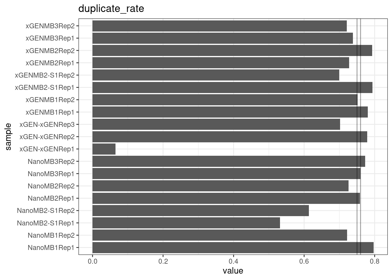
Fraction of single-read families
Shows the number of single-read families divided by the total number of reads. As suggested by Stoler et al. 2016, this metric can server as a proxy for error rate, as (uncorrected) barcode mismatches will manifest as single-read families. The lower the fraction of singletons, the better.
metric <- 'frac_singletons'
ggplot(mm[mm$metric == metric,], aes(sample, value)) +
        geom_histogram(stat = 'identity', position = 'dodge') +
        theme_bw() +
        coord_flip() +
        ggtitle(metric)
Drop-out rate
This is the same calculation as F-EFF in the NanoSeq Analysis pipeline:
“This shows the fraction of read bundles missing one of the two original strands beyond what would be expected under random sampling (assuming a binomial process). Good values are between 0.10-0.30, and larger values are likely due to DNA damage such as modified bases or internal nicks that prevent amplification of one of the two strands. Larger values do not impact the quality of the results, just reduce the efficiency of the protocol.”
This is similar to the singleton fraction, but taking into account loss of pairs due to sampling. The optimal range is shown by the lines.
metric <- 'drop_out_rate'
ggplot(mm[mm$metric == metric,], aes(sample, value)) +
        geom_histogram(stat = 'identity', position = 'dodge') +
        theme_bw() +
        coord_flip() +
        geom_hline(yintercept = c(0.1, 0.3), alpha = 0.4)  +
        ggtitle(metric)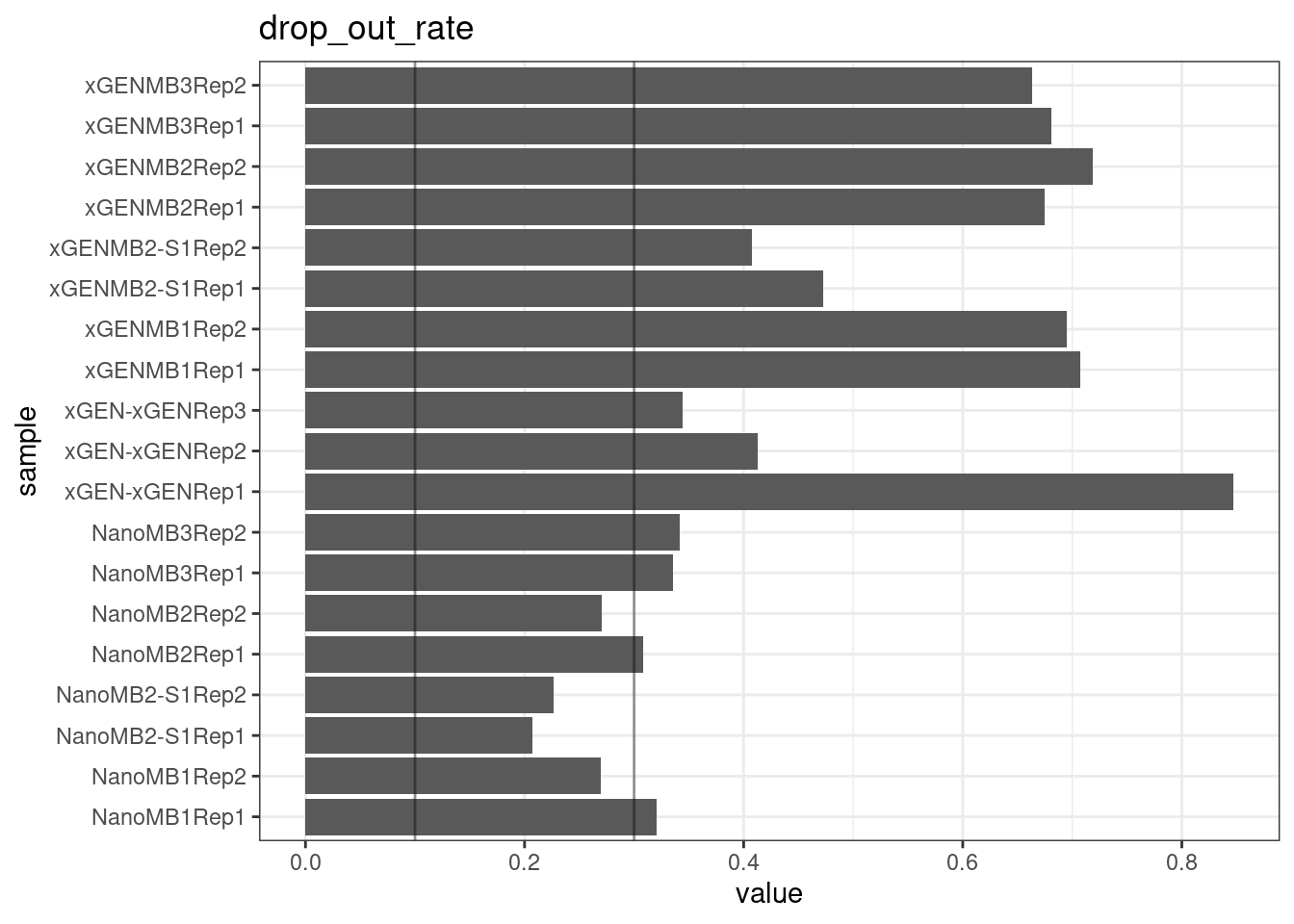
Efficiency
Efficiency is the number of duplex bases divided by the number of sequenced bases. According the NanoSeq Analysis pipeline, this value is maximised at ~0.07 when duplicate rates and strand drop-outs are optimal.
metric <- 'efficiency'
ggplot(mm[mm$metric == metric,], aes(sample, value)) +
        geom_histogram(stat = 'identity', position = 'dodge') +
        theme_bw() +
        coord_flip() +
        geom_hline(yintercept = c(0.07), alpha = 0.4)  +
        ggtitle(metric)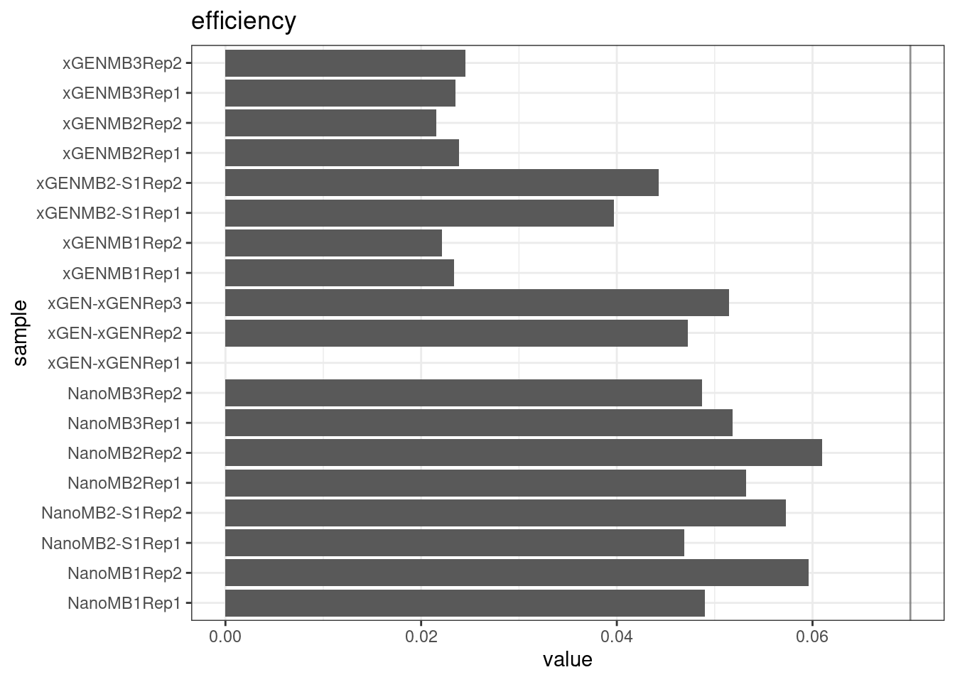
GC deviation
GC deviation is the absolute difference between GC_BOTH and GC_SINGLE calculated by the NanoSeq Analysis pipeline. The lower this deviation, the better.
“GC_BOTH and GC_SINGLE: the GC content of RBs with both strands and with just one strand. The two values should be similar between them and similar to the genome average. If there are large deviations that is possibly due to biases during PCR amplification. If GC_BOTH is substantially larger than GC_SINGLE, DNA denaturation before dilution may have taken place.”
metric <- 'gc_deviation'
ggplot(mm[mm$metric == metric,], aes(sample, value)) +
        geom_histogram(stat = 'identity', position = 'dodge') +
        theme_bw() +
        coord_flip() +
        geom_hline(yintercept = c(0.07), alpha = 0.4)  +
        ggtitle(metric)
Duplex Coverage ratio
The mean sequence (pre-duplex) coverage divided by mean duplex coverage. Indicates the yield of how much duplex coverage we get at each sample’s sequence coverage. Abascal et al. report that their yield was approximately 30x (marked on the plot).
metric <- 'duplex_coverage_ratio'
ggplot(mm[mm$metric == metric,], aes(sample, value)) +
        geom_histogram(stat = 'identity', position = 'dodge') +
        theme_bw() +
        coord_flip() +
        geom_hline(yintercept = 30, alpha = 0.4)  +
        ggtitle(metric)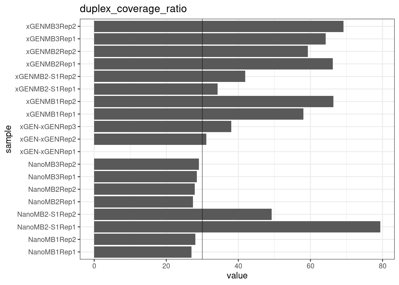
Compare metrics side-by-side
Compare protocols and nucleases directly.
# duplicate rate
p1 <- plot_metric_boxplot(mm, 'protocol', 'duplicate_rate', 'Duplicate rate (line = optimal)') +
    geom_jitter(width=0.1, aes(protocol, value, colour = nuclease)) +
    geom_hline(yintercept = 0.81) +
    theme(legend.position = 'bottom')

p2 <- plot_metric_boxplot(mm, 'nuclease', 'duplicate_rate', 'Duplicate rate (line = optimal)') +
    geom_jitter(width=0.1, aes(nuclease, value, colour = protocol)) +
    geom_hline(yintercept = 0.81) +
    theme(legend.position = 'bottom')

show(p1 + p2)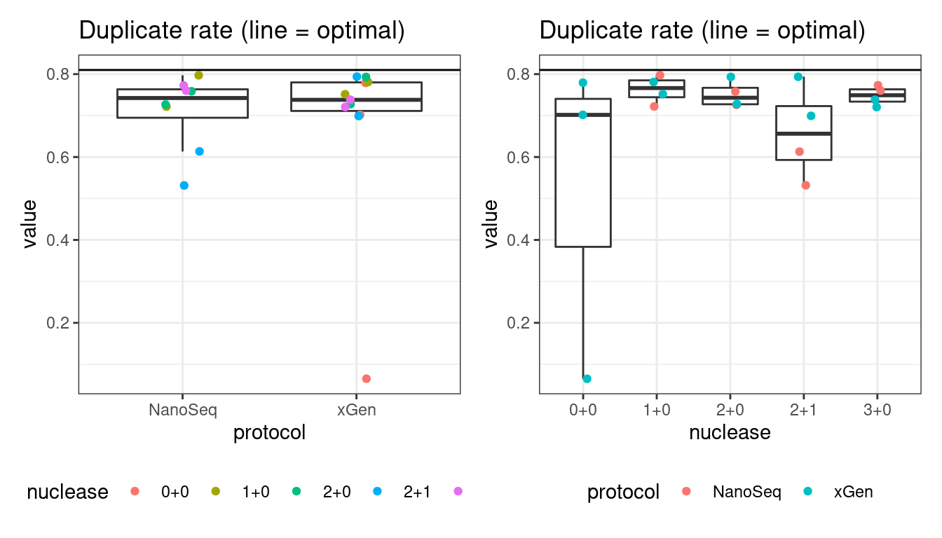
# singletons
p1 <- plot_metric_boxplot(mm, 'protocol', 'frac_singletons', 'Fraction of singleton reads') +
    geom_jitter(width=0.1, aes(protocol, value, colour = nuclease)) +
    theme(legend.position = 'bottom') +
    ylim(c(0,1))

p2 <- plot_metric_boxplot(mm, 'nuclease', 'frac_singletons', 'Fraction of singleton reads') +
    geom_jitter(width=0.1, aes(nuclease, value, colour = protocol))  +
    theme(legend.position = 'bottom') +
    ylim(c(0,1))

show(p1 + p2)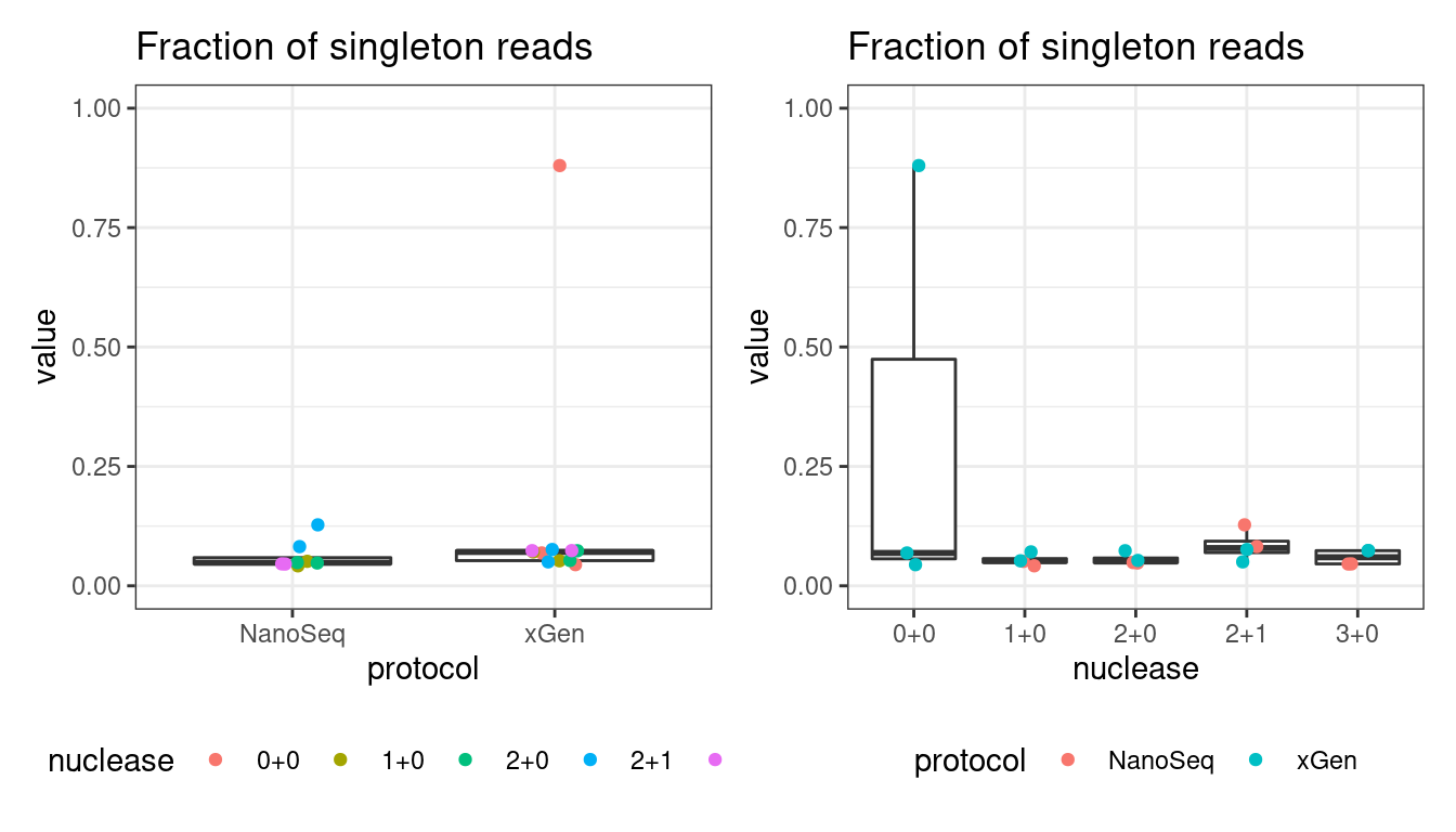
# drop out rate
p1 <- plot_metric_boxplot(mm, 'protocol', 'drop_out_rate', 'Strand drop-out fraction (lines = optimal range)') +
    geom_jitter(width=0.1, aes(protocol, value, colour = nuclease)) +
    geom_hline(yintercept = c(0.1, 0.3)) +
    theme(legend.position = 'bottom') +
    ylim(c(0,1))


p2 <- plot_metric_boxplot(mm, 'nuclease', 'drop_out_rate', 'Strand drop-out fraction (lines = optimal range)') +
    geom_jitter(width=0.1, aes(nuclease, value, colour = protocol)) +
    geom_hline(yintercept = c(0.1, 0.3)) +
    theme(legend.position = 'bottom') +
    ylim(c(0,1))

show(p1 + p2)
# efficiency
p1 <- plot_metric_boxplot(mm, 'protocol', 'efficiency', 'Efficiency (line = optimal)') +
    geom_jitter(width=0.1, aes(protocol, value, colour = nuclease)) +
    geom_hline(yintercept = 0.07) +
    theme(legend.position = 'bottom')

p2 <- plot_metric_boxplot(mm, 'nuclease', 'efficiency', 'Efficiency (line = optimal)') +
    geom_jitter(width=0.1, aes(nuclease, value, colour = protocol)) +
    geom_hline(yintercept = 0.07) +
    theme(legend.position = 'bottom')

show(p1 + p2)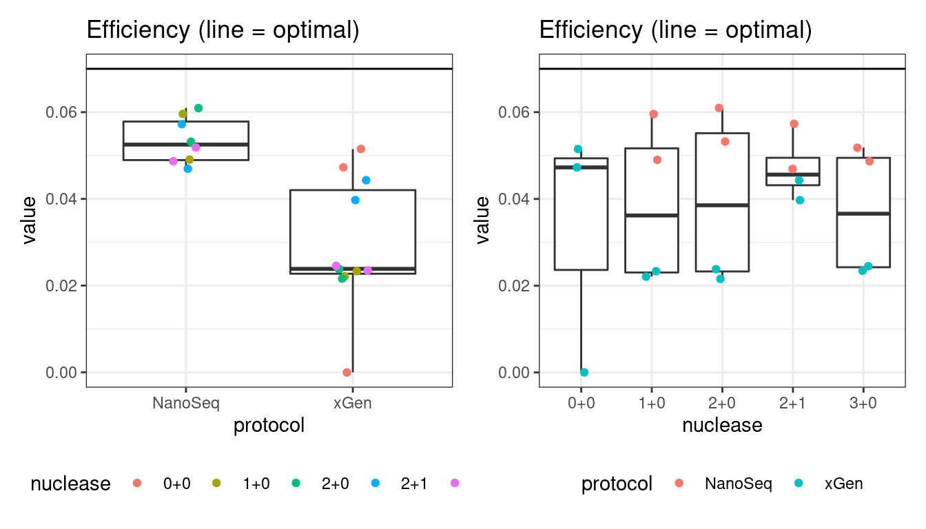
# GC deviation between strands
p1 <- plot_metric_boxplot(mm, 'protocol', 'gc_deviation', 'GC deviation (both strands vs. one)') +
    geom_jitter(width=0.1, aes(protocol, value, colour = nuclease)) +
    theme(legend.position = 'bottom')

p2 <- plot_metric_boxplot(mm, 'nuclease', 'gc_deviation', 'GC deviation (both strands vs. one)') +
    geom_jitter(width=0.1, aes(nuclease, value, colour = protocol)) +
    theme(legend.position = 'bottom')

show(p1 + p2)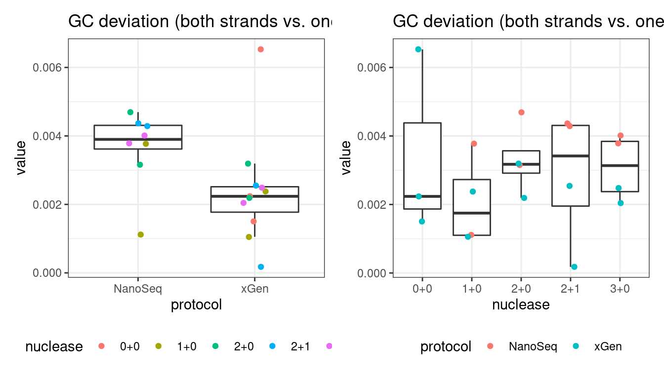
# duplex coverage ratio
p1 <- plot_metric_boxplot(mm, 'protocol', 'duplex_coverage_ratio', 'Duplex coverage ratio (total cov / duplex cov)') +
    geom_jitter(width=0.1, aes(protocol, value, colour = nuclease)) +
    geom_hline(yintercept = 30) +
    theme(legend.position = 'bottom')

p2 <- plot_metric_boxplot(mm, 'nuclease', 'duplex_coverage_ratio', 'Duplex coverage ratio (total cov / duplex cov)') +
    geom_jitter(width=0.1, aes(nuclease, value, colour = protocol)) +
    geom_hline(yintercept = 30) +
    theme(legend.position = 'bottom')

show(p1 + p2)
Facet summary plots
Facet boxplots by nuclease and protocol to show overall results.
ggplot(mm, aes(protocol, value)) +
    geom_boxplot() +
    theme_bw() +
    facet_wrap(~metric, scales = 'free') +
    ggtitle('by protocol')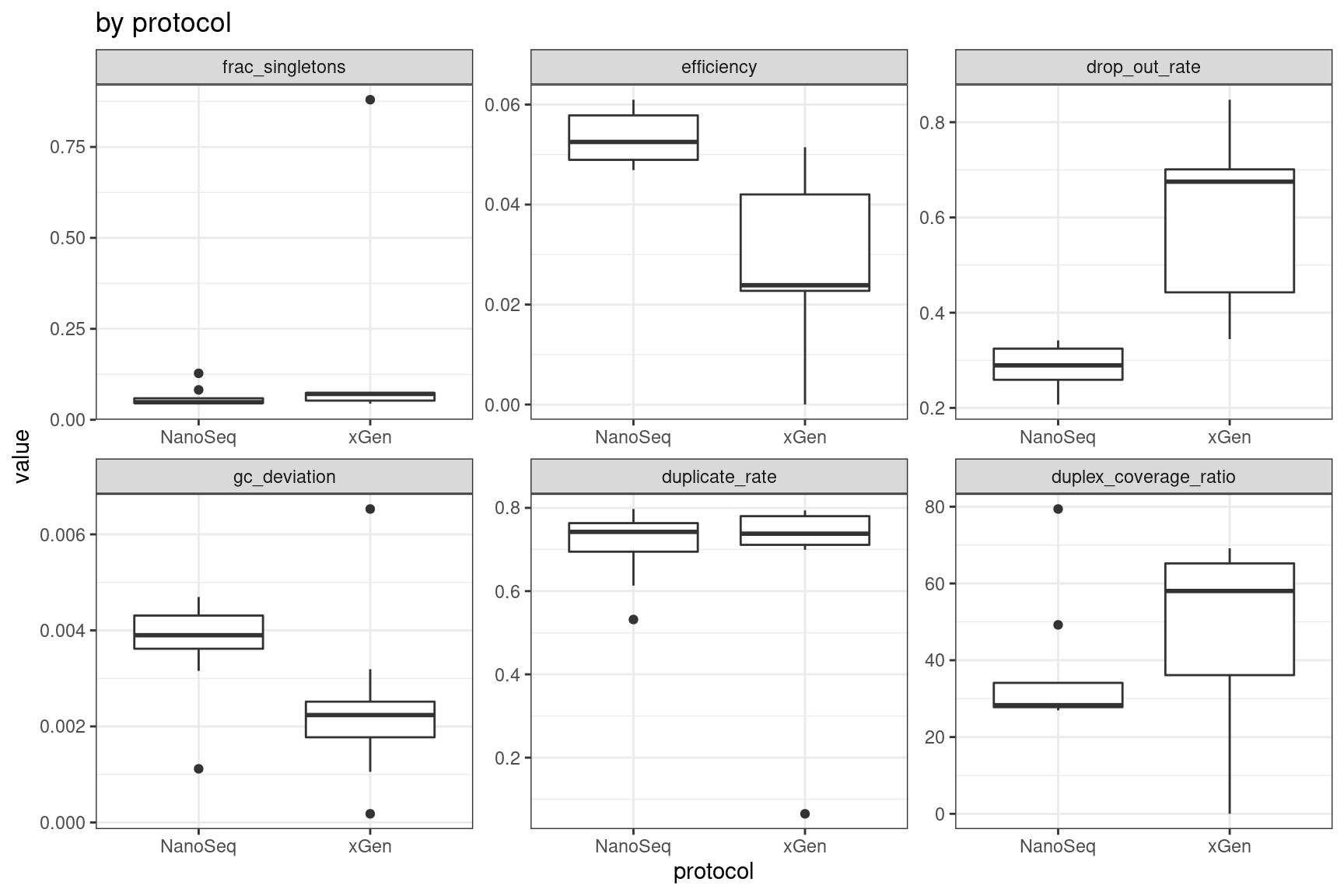
ggplot(mm, aes(nuclease, value)) +
    geom_boxplot() +
    theme_bw() +
    facet_wrap(~metric, scales = 'free') +
    ggtitle('by nuclease')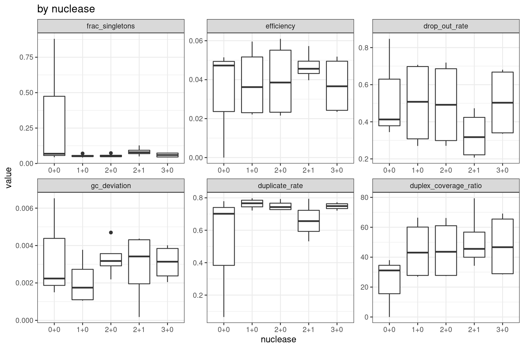
Statistical test results by protocol
For each metric, take the average of each replicate and perform a two-sided, unpaired T-test between protocols.
stats <- NULL
metric_names <- unique(mm$metric) %>% as.character()
for(metric_name in metric_names) {
    nano <- mm[mm$metric == metric_name & mm$protocol == 'NanoSeq',]
    xgen <- mm[mm$metric == metric_name & mm$protocol == 'xGen',]
    nano_vals <- data.table(nano)[, mean(value), by = nuclease]$V1
    xgen_vals <- data.table(xgen)[, mean(value), by = nuclease]$V1
    wtest <- t.test(nano_vals, xgen_vals)
    stats <- rbind(stats,
                   data.frame(metric = metric_name, pvalue = wtest$p.value))
}
stats$significant <- stats$pvalue < 0.05
print(stats)
metric pvalue significant
1 frac_singletons 0.350920599 FALSE
2 efficiency 0.001645545 TRUE
3 drop_out_rate 0.001656330 TRUE
4 gc_deviation 0.045504038 TRUE
5 duplicate_rate 0.922536682 FALSE
6 duplex_coverage_ratio 0.316697444 FALSETwo-way ANOVA analysis
We consider a two-way ANOVA, modelling the protocol, Mung Bean Unit and S1 Unit variables, as well as the interaction effect between the units and the protocol.
stats <- NULL
metric_names <- unique(mm$metric) %>% as.character()
for(metric_name in metric_names) {
    x <- mm[mm$metric == metric_name,]
    x$MungBeanUnit <- as.factor(x$`Mung bean unit`)
    x$S1Unit <- as.factor(x$`S1 unit`)
    x <- x[,c('MungBeanUnit', 'S1Unit', 'protocol', 'nuclease', 'value')]
    x_aov <- aov(value ~ MungBeanUnit * protocol + S1Unit * protocol, data = x) %>% summary() %>% dplyr::first()
    stats <- rbind(stats,
                   data.frame(metric = metric_name,
                              variable = rownames(x_aov)[1:5],
                              pvalue = x_aov[['Pr(>F)']][1:5]))
}
stats$significant <- stats$pvalue < 0.05
print(stats)
metric variable pvalue significant
1 frac_singletons MungBeanUnit 0.3179447536 FALSE
2 frac_singletons protocol 0.9702278541 FALSE
3 frac_singletons S1Unit 0.8553539457 FALSE
4 frac_singletons MungBeanUnit:protocol 0.9858376372 FALSE
5 frac_singletons protocol:S1Unit 0.8540792709 FALSE
6 efficiency MungBeanUnit 0.6743588660 FALSE
7 efficiency protocol 0.0033776091 TRUE
8 efficiency S1Unit 0.4674622674 FALSE
9 efficiency MungBeanUnit:protocol 0.8509682597 FALSE
10 efficiency protocol:S1Unit 0.2278366157 FALSE
11 drop_out_rate MungBeanUnit 0.4118682293 FALSE
12 drop_out_rate protocol 0.0002566346 TRUE
13 drop_out_rate S1Unit 0.0904262242 FALSE
14 drop_out_rate MungBeanUnit:protocol 0.8387881526 FALSE
15 drop_out_rate protocol:S1Unit 0.3182162279 FALSE
16 gc_deviation MungBeanUnit 0.6632789428 FALSE
17 gc_deviation protocol 0.0591657318 FALSE
18 gc_deviation S1Unit 0.6799659214 FALSE
19 gc_deviation MungBeanUnit:protocol 0.7726060695 FALSE
20 gc_deviation protocol:S1Unit 0.4452940513 FALSE
21 duplicate_rate MungBeanUnit 0.3209743574 FALSE
22 duplicate_rate protocol 0.6617113407 FALSE
23 duplicate_rate S1Unit 0.4855983121 FALSE
24 duplicate_rate MungBeanUnit:protocol 0.8160371321 FALSE
25 duplicate_rate protocol:S1Unit 0.5516726318 FALSE
26 duplex_coverage_ratio MungBeanUnit 0.0515969116 FALSE
27 duplex_coverage_ratio protocol 0.0059993368 TRUE
28 duplex_coverage_ratio S1Unit 0.4875101164 FALSE
29 duplex_coverage_ratio MungBeanUnit:protocol 0.0621558351 FALSE
30 duplex_coverage_ratio protocol:S1Unit 0.0041291841 TRUERelationships between variables
mm$replicate <- str_split(mm$sample, 'Rep') %>% lapply(., dplyr::last) %>% unlist() %>% as.numeric()
mm$sample <- str_split(mm$sample, 'Rep') %>% lapply(., dplyr::first) %>% unlist()

mm <- mm[,c('sample', 'metric', 'value', 'protocol', 'nuclease', 'replicate')]
dm <- reshape2::dcast(mm, sample + protocol + nuclease + replicate ~ metric)

cols <- c(brewer.pal(5, 'Greens')[2:5],
          brewer.pal(6, 'Blues')[2:6])
names(cols) <- as.factor(dm$sample) %>% levels()

ggplot(dm, aes(frac_singletons, drop_out_rate, colour=sample)) +
    geom_point() +
    theme_bw() +
    scale_colour_manual(values = cols) +
    ggtitle('Singletons vs. drop-out rate')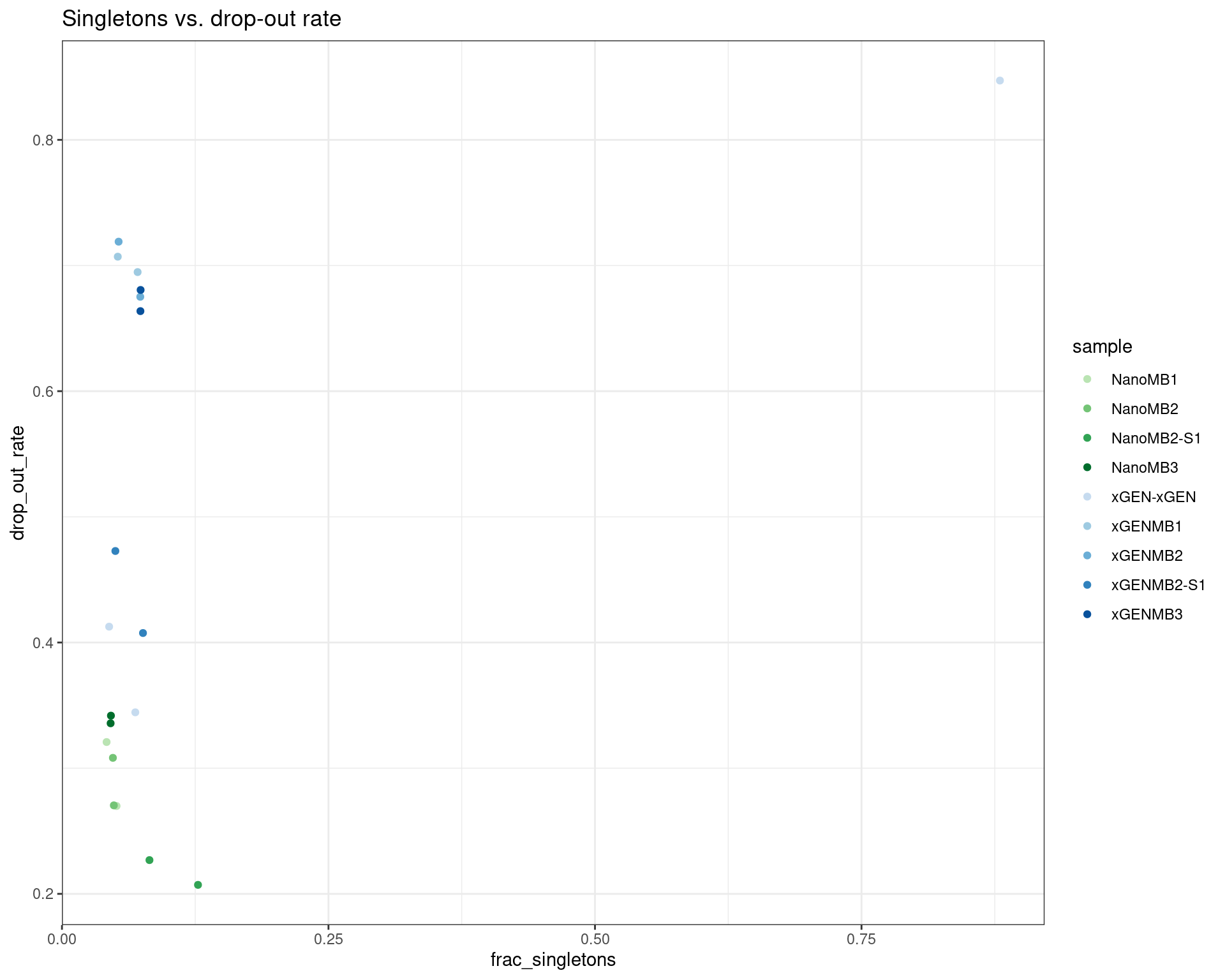
ggplot(dm, aes(efficiency, duplicate_rate, colour=sample)) +
    geom_point() +
    theme_bw() +
    scale_colour_manual(values = cols) +
    ggtitle('Efficiency vs. duplicate rate')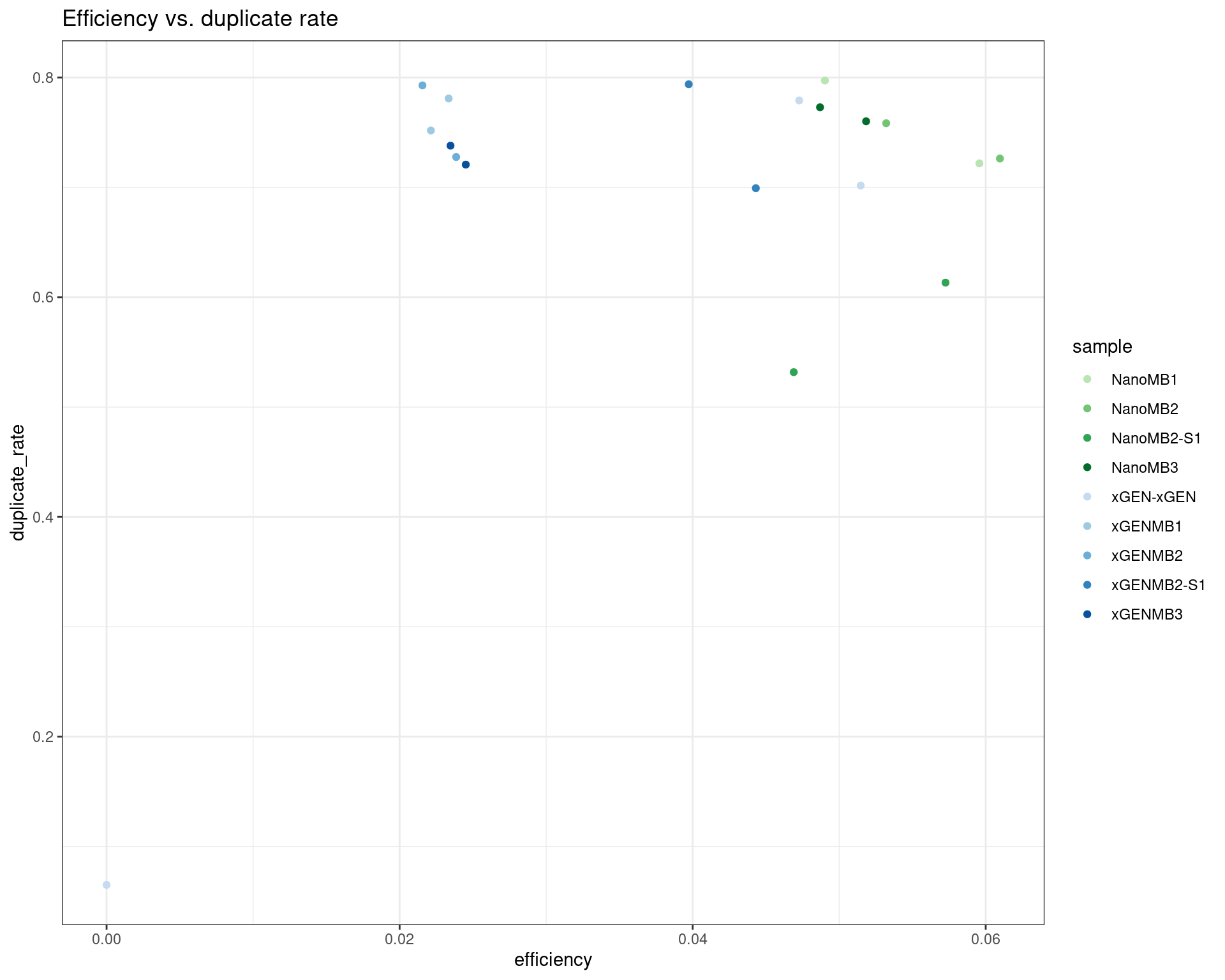
ggplot(dm, aes(efficiency, drop_out_rate, colour=sample)) +
    geom_point() +
    theme_bw() +
    scale_colour_manual(values = cols) +
    ggtitle('Efficiency vs. drop-out rate')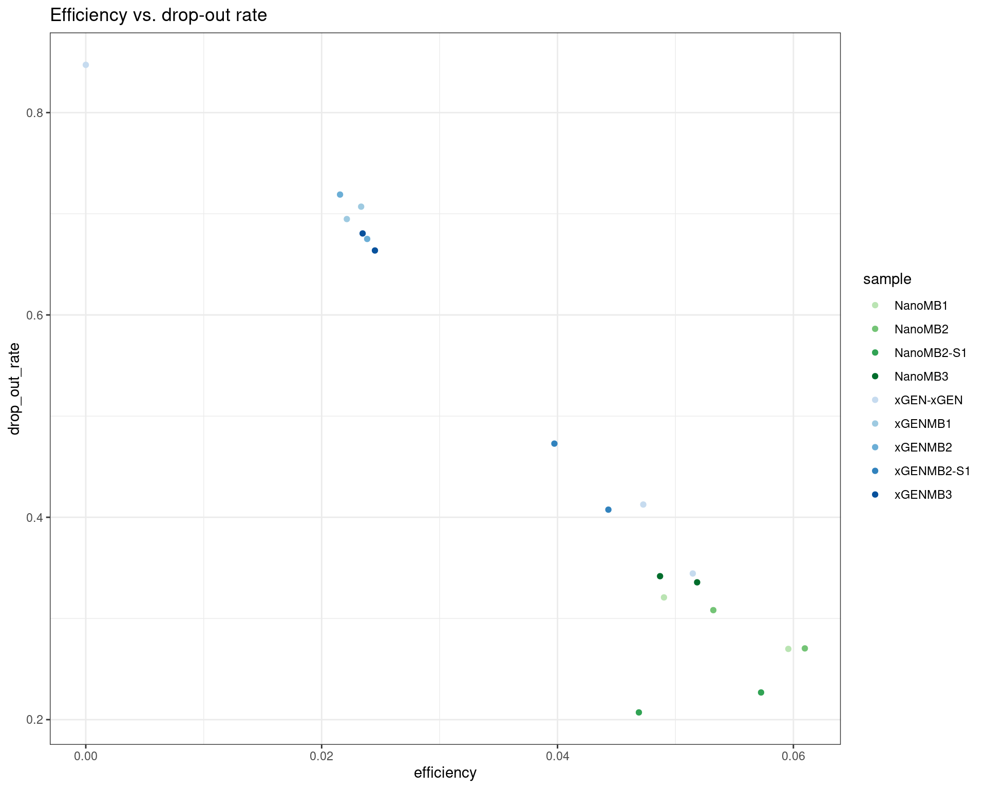
ggplot(dm, aes(efficiency, duplex_coverage_ratio, colour=sample)) +
    geom_point() +
    theme_bw() +
    scale_colour_manual(values = cols) +
    ggtitle('Efficiency vs. duplex coverage ratio')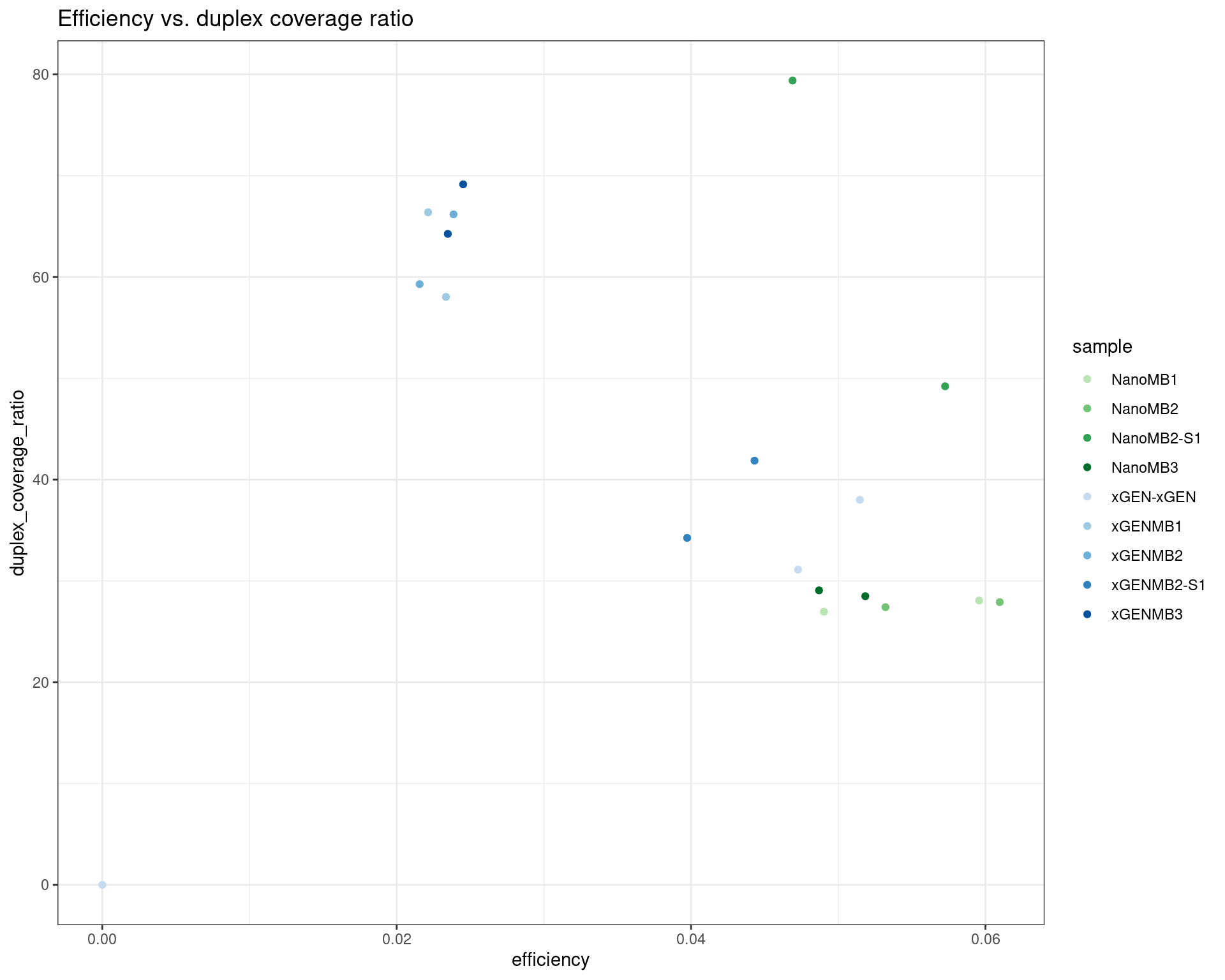
ggplot(dm, aes(duplicate_rate, duplex_coverage_ratio, colour=sample)) +
    geom_point() +
    theme_bw() +
    scale_colour_manual(values = cols) +
    ggtitle('Duplicate rate vs. duplex coverage ratio')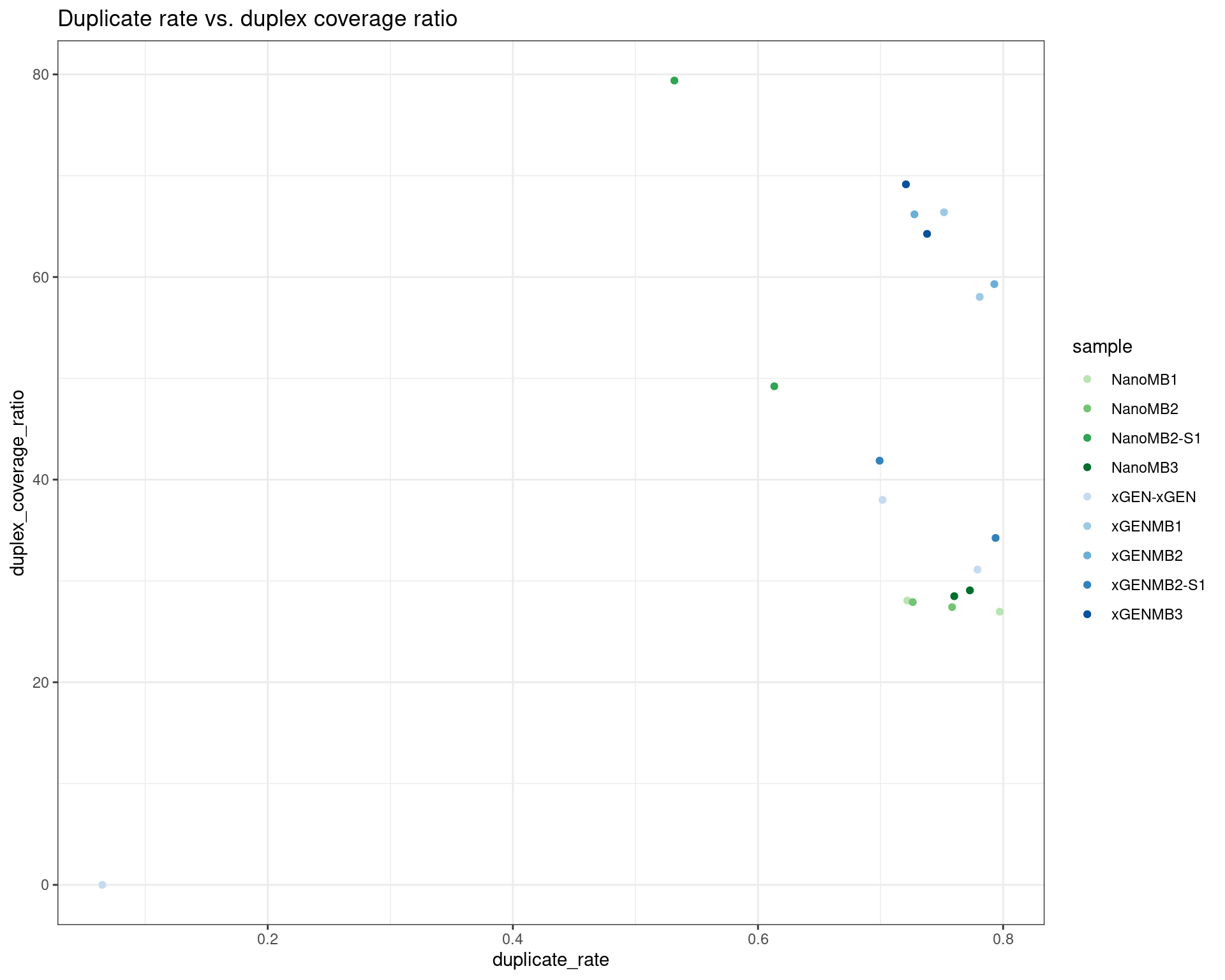
sessionInfo()R version 4.0.5 (2021-03-31)
Platform: x86_64-pc-linux-gnu (64-bit)
Running under: CentOS Linux 7 (Core)
Matrix products: default
BLAS: /stornext/System/data/apps/R/R-4.0.5/lib64/R/lib/libRblas.so
LAPACK: /stornext/System/data/apps/R/R-4.0.5/lib64/R/lib/libRlapack.so
locale:
[1] LC_CTYPE=en_US.UTF-8 LC_NUMERIC=C
[3] LC_TIME=en_US.UTF-8 LC_COLLATE=en_US.UTF-8
[5] LC_MONETARY=en_US.UTF-8 LC_MESSAGES=en_US.UTF-8
[7] LC_PAPER=en_US.UTF-8 LC_NAME=C
[9] LC_ADDRESS=C LC_TELEPHONE=C
[11] LC_MEASUREMENT=en_US.UTF-8 LC_IDENTIFICATION=C
attached base packages:
[1] stats4 parallel stats graphics grDevices utils datasets
[8] methods base
other attached packages:
[1] RColorBrewer_1.1-2 patchwork_1.1.1 readxl_1.3.1
[4] seqinr_4.2-8 Rsamtools_2.6.0 Biostrings_2.58.0
[7] XVector_0.30.0 GenomicRanges_1.42.0 GenomeInfoDb_1.26.7
[10] IRanges_2.24.1 S4Vectors_0.28.1 BiocGenerics_0.36.1
[13] stringr_1.4.0 tibble_3.1.5 here_1.0.1
[16] dplyr_1.0.7 data.table_1.14.0 ggplot2_3.3.5
[19] workflowr_1.6.2
loaded via a namespace (and not attached):
[1] Rcpp_1.0.7 assertthat_0.2.1 rprojroot_2.0.2
[4] digest_0.6.27 utf8_1.2.2 plyr_1.8.6
[7] cellranger_1.1.0 R6_2.5.1 evaluate_0.14
[10] highr_0.9 pillar_1.6.4 zlibbioc_1.36.0
[13] rlang_0.4.12 whisker_0.4 jquerylib_0.1.4
[16] rmarkdown_2.11 labeling_0.4.2 BiocParallel_1.24.1
[19] RCurl_1.98-1.3 munsell_0.5.0 compiler_4.0.5
[22] httpuv_1.6.3 xfun_0.22 pkgconfig_2.0.3
[25] htmltools_0.5.2 tidyselect_1.1.1 GenomeInfoDbData_1.2.4
[28] fansi_0.5.0 crayon_1.4.2 withr_2.4.2
[31] later_1.3.0 MASS_7.3-53.1 bitops_1.0-7
[34] grid_4.0.5 jsonlite_1.7.2 gtable_0.3.0
[37] lifecycle_1.0.1 DBI_1.1.1 git2r_0.28.0
[40] magrittr_2.0.1 scales_1.1.1 stringi_1.7.5
[43] farver_2.1.0 reshape2_1.4.4 fs_1.5.0
[46] promises_1.2.0.1 bslib_0.3.0 ellipsis_0.3.2
[49] generics_0.1.1 vctrs_0.3.8 tools_4.0.5
[52] ade4_1.7-18 glue_1.4.2 purrr_0.3.4
[55] fastmap_1.1.0 yaml_2.2.1 colorspace_2.0-0
[58] knitr_1.33 sass_0.4.0