Supplementary figures
ERM
2023-08-10
Last updated: 2023-08-10
Checks: 7 0
Knit directory: Cardiotoxicity/
This reproducible R Markdown analysis was created with workflowr (version 1.7.0). The Checks tab describes the reproducibility checks that were applied when the results were created. The Past versions tab lists the development history.
Great! Since the R Markdown file has been committed to the Git repository, you know the exact version of the code that produced these results.
Great job! The global environment was empty. Objects defined in the global environment can affect the analysis in your R Markdown file in unknown ways. For reproduciblity it’s best to always run the code in an empty environment.
The command set.seed(20230109) was run prior to running
the code in the R Markdown file. Setting a seed ensures that any results
that rely on randomness, e.g. subsampling or permutations, are
reproducible.
Great job! Recording the operating system, R version, and package versions is critical for reproducibility.
Nice! There were no cached chunks for this analysis, so you can be confident that you successfully produced the results during this run.
Great job! Using relative paths to the files within your workflowr project makes it easier to run your code on other machines.
Great! You are using Git for version control. Tracking code development and connecting the code version to the results is critical for reproducibility.
The results in this page were generated with repository version b30e0e4. See the Past versions tab to see a history of the changes made to the R Markdown and HTML files.
Note that you need to be careful to ensure that all relevant files for
the analysis have been committed to Git prior to generating the results
(you can use wflow_publish or
wflow_git_commit). workflowr only checks the R Markdown
file, but you know if there are other scripts or data files that it
depends on. Below is the status of the Git repository when the results
were generated:
Ignored files:
    Ignored:    .RData
    Ignored:    .Rhistory
    Ignored:    .Rproj.user/
    Ignored:    data/41588_2018_171_MOESM3_ESMeQTL_ST2_for paper.csv
    Ignored:    data/Arr_GWAS.txt
    Ignored:    data/Arr_geneset.RDS
    Ignored:    data/BC_cell_lines.csv
    Ignored:    data/BurridgeDOXTOX.RDS
    Ignored:    data/CADGWASgene_table.csv
    Ignored:    data/CAD_geneset.RDS
    Ignored:    data/CALIMA_Data/
    Ignored:    data/Clamp_Summary.csv
    Ignored:    data/Cormotif_24_k1-5_raw.RDS
    Ignored:    data/DAgostres24.RDS
    Ignored:    data/DAtable1.csv
    Ignored:    data/DDEMresp_list.csv
    Ignored:    data/DDE_reQTL.txt
    Ignored:    data/DDEresp_list.csv
    Ignored:    data/DEG-GO/
    Ignored:    data/DEG_cormotif.RDS
    Ignored:    data/DF_Plate_Peak.csv
    Ignored:    data/DRC48hoursdata.csv
    Ignored:    data/Da24counts.txt
    Ignored:    data/Dx24counts.txt
    Ignored:    data/Dx_reQTL_specific.txt
    Ignored:    data/Ep24counts.txt
    Ignored:    data/Full_LD_rep.csv
    Ignored:    data/GOIsig.csv
    Ignored:    data/GOplots.R
    Ignored:    data/GTEX_setsimple.csv
    Ignored:    data/GTEX_sig24.RDS
    Ignored:    data/GTEx_gene_list.csv
    Ignored:    data/HFGWASgene_table.csv
    Ignored:    data/HF_geneset.RDS
    Ignored:    data/Heart_Left_Ventricle.v8.egenes.txt
    Ignored:    data/Heatmap_mat.RDS
    Ignored:    data/Heatmap_sig.RDS
    Ignored:    data/Hf_GWAS.txt
    Ignored:    data/K_cluster
    Ignored:    data/K_cluster_kisthree.csv
    Ignored:    data/K_cluster_kistwo.csv
    Ignored:    data/LD50_05via.csv
    Ignored:    data/LDH48hoursdata.csv
    Ignored:    data/Mt24counts.txt
    Ignored:    data/NoRespDEG_final.csv
    Ignored:    data/RINsamplelist.txt
    Ignored:    data/Seonane2019supp1.txt
    Ignored:    data/TMMnormed_x.RDS
    Ignored:    data/TOP2Bi-24hoursGO_analysis.csv
    Ignored:    data/TR24counts.txt
    Ignored:    data/Top2biresp_cluster24h.csv
    Ignored:    data/Var_test_list.RDS
    Ignored:    data/Var_test_list24.RDS
    Ignored:    data/Var_test_list24alt.RDS
    Ignored:    data/Var_test_list3.RDS
    Ignored:    data/Viabilitylistfull.csv
    Ignored:    data/allexpressedgenes.txt
    Ignored:    data/allfinal3hour.RDS
    Ignored:    data/allgenes.txt
    Ignored:    data/allmatrix.RDS
    Ignored:    data/allmymatrix.RDS
    Ignored:    data/annotation_data_frame.RDS
    Ignored:    data/averageviabilitytable.RDS
    Ignored:    data/avgLD50.RDS
    Ignored:    data/avg_LD50.RDS
    Ignored:    data/backGL.txt
    Ignored:    data/burr_genes.RDS
    Ignored:    data/calcium_data.RDS
    Ignored:    data/clamp_summary.RDS
    Ignored:    data/cormotif_3hk1-8.RDS
    Ignored:    data/cormotif_initalK5.RDS
    Ignored:    data/cormotif_initialK5.RDS
    Ignored:    data/cormotif_initialall.RDS
    Ignored:    data/counts24hours.RDS
    Ignored:    data/cpmcount.RDS
    Ignored:    data/cpmnorm_counts.csv
    Ignored:    data/crispr_genes.csv
    Ignored:    data/ctnnt_results.txt
    Ignored:    data/cvd_GWAS.txt
    Ignored:    data/dat_cpm.RDS
    Ignored:    data/data_outline.txt
    Ignored:    data/drug_noveh1.csv
    Ignored:    data/efit2.RDS
    Ignored:    data/efit2_final.RDS
    Ignored:    data/efit2results.RDS
    Ignored:    data/ensembl_backup.RDS
    Ignored:    data/ensgtotal.txt
    Ignored:    data/filcpm_counts.RDS
    Ignored:    data/filenameonly.txt
    Ignored:    data/filtered_cpm_counts.csv
    Ignored:    data/filtered_raw_counts.csv
    Ignored:    data/filtermatrix_x.RDS
    Ignored:    data/folder_05top/
    Ignored:    data/geneDoxonlyQTL.csv
    Ignored:    data/gene_corr_df.RDS
    Ignored:    data/gene_corr_frame.RDS
    Ignored:    data/gene_prob_tran3h.RDS
    Ignored:    data/gene_probabilityk5.RDS
    Ignored:    data/geneset_24.RDS
    Ignored:    data/gostresTop2bi_ER.RDS
    Ignored:    data/gostresTop2bi_LR
    Ignored:    data/gostresTop2bi_LR.RDS
    Ignored:    data/gostresTop2bi_TI.RDS
    Ignored:    data/gostrescoNR
    Ignored:    data/gtex/
    Ignored:    data/heartgenes.csv
    Ignored:    data/hsa_kegg_anno.RDS
    Ignored:    data/individualDRCfile.RDS
    Ignored:    data/individual_DRC48.RDS
    Ignored:    data/individual_LDH48.RDS
    Ignored:    data/indv_noveh1.csv
    Ignored:    data/kegglistDEG.RDS
    Ignored:    data/kegglistDEG24.RDS
    Ignored:    data/kegglistDEG3.RDS
    Ignored:    data/knowfig4.csv
    Ignored:    data/knowfig5.csv
    Ignored:    data/label_list.RDS
    Ignored:    data/ld50_table.csv
    Ignored:    data/mean_vardrug1.csv
    Ignored:    data/mean_varframe.csv
    Ignored:    data/mymatrix.RDS
    Ignored:    data/new_ld50avg.RDS
    Ignored:    data/nonresponse_cluster24h.csv
    Ignored:    data/norm_LDH.csv
    Ignored:    data/norm_counts.csv
    Ignored:    data/old_sets/
    Ignored:    data/organized_drugframe.csv
    Ignored:    data/plan2plot.png
    Ignored:    data/plot_intv_list.RDS
    Ignored:    data/plot_list_DRC.RDS
    Ignored:    data/qval24hr.RDS
    Ignored:    data/qval3hr.RDS
    Ignored:    data/qvalueEPItemp.RDS
    Ignored:    data/raw_counts.csv
    Ignored:    data/response_cluster24h.csv
    Ignored:    data/sigVDA24.txt
    Ignored:    data/sigVDA3.txt
    Ignored:    data/sigVDX24.txt
    Ignored:    data/sigVDX3.txt
    Ignored:    data/sigVEP24.txt
    Ignored:    data/sigVEP3.txt
    Ignored:    data/sigVMT24.txt
    Ignored:    data/sigVMT3.txt
    Ignored:    data/sigVTR24.txt
    Ignored:    data/sigVTR3.txt
    Ignored:    data/siglist.RDS
    Ignored:    data/siglist_final.RDS
    Ignored:    data/siglist_old.RDS
    Ignored:    data/slope_table.csv
    Ignored:    data/supp10_24hlist.RDS
    Ignored:    data/supp10_3hlist.RDS
    Ignored:    data/supp_normLDH48.RDS
    Ignored:    data/supp_pca_all_anno.RDS
    Ignored:    data/table3a.omar
    Ignored:    data/testlist.txt
    Ignored:    data/toplistall.RDS
    Ignored:    data/trtonly_24h_genes.RDS
    Ignored:    data/trtonly_3h_genes.RDS
    Ignored:    data/tvl24hour.txt
    Ignored:    data/tvl24hourw.txt
    Ignored:    data/venn_code.R
    Ignored:    data/viability.RDS

Untracked files:
    Untracked:  .RDataTmp
    Untracked:  .RDataTmp1
    Untracked:  .RDataTmp2
    Untracked:  Doxorubicin_vehicle_3_24.csv
    Untracked:  Doxtoplist.csv
    Untracked:  GWAS_list_of_interest.xlsx
    Untracked:  KEGGpathwaylist.R
    Untracked:  OmicNavigator_learn.R
    Untracked:  SigDoxtoplist.csv
    Untracked:  analysis/DRC_analysist.Rmd
    Untracked:  analysis/ciFIT.R
    Untracked:  analysis/enricher.Rmd
    Untracked:  analysis/export_to_excel.R
    Untracked:  analysis/untitled1.R
    Untracked:  code/DRC_plotfigure1.png
    Untracked:  code/constantcode.R
    Untracked:  code/cpm_boxplot.R
    Untracked:  code/extracting_ggplot_data.R
    Untracked:  code/fig1plot.png
    Untracked:  code/figurelegeddrc.png
    Untracked:  code/movingfilesto_ppl.R
    Untracked:  code/pearson_extract_func.R
    Untracked:  code/pearson_tox_extract.R
    Untracked:  code/plot1C.fun.R
    Untracked:  code/spearman_extract_func.R
    Untracked:  code/venndiagramcolor_control.R
    Untracked:  cormotif_probability_genelist.csv
    Untracked:  individual-legenddark2.png
    Untracked:  installed_old.rda
    Untracked:  motif_ER.txt
    Untracked:  motif_LR.txt
    Untracked:  motif_NR.txt
    Untracked:  motif_TI.txt
    Untracked:  output/DNRvenn.RDS
    Untracked:  output/DOXvenn.RDS
    Untracked:  output/EPIvenn.RDS
    Untracked:  output/Figures/
    Untracked:  output/MTXvenn.RDS
    Untracked:  output/Volcanoplot_10
    Untracked:  output/Volcanoplot_10.RDS
    Untracked:  output/allfinal_sup10.RDS
    Untracked:  output/gene_corr_fig9.RDS
    Untracked:  output/legend_b.RDS
    Untracked:  output/motif_ERrep.RDS
    Untracked:  output/motif_LRrep.RDS
    Untracked:  output/motif_NRrep.RDS
    Untracked:  output/motif_TI_rep.RDS
    Untracked:  output/output-old/
    Untracked:  output/rank24genes.csv
    Untracked:  output/rank3genes.csv
    Untracked:  output/supplementary_motif_list_GO.RDS
    Untracked:  output/toptablebydrug.RDS
    Untracked:  output/x_counts.RDS
    Untracked:  reneebasecode.R

Unstaged changes:
    Modified:   analysis/Figure5.Rmd
    Modified:   analysis/Knowles2019.Rmd
    Modified:   analysis/variance_scrip.Rmd
    Modified:   output/TNNI_LDH_RNAnormlist.txt
    Modified:   output/daplot.RDS
    Modified:   output/dxplot.RDS
    Modified:   output/epplot.RDS
    Modified:   output/mtplot.RDS
    Modified:   output/plan2plot.png
    Modified:   output/toplistall.csv
    Modified:   output/trplot.RDS
    Modified:   output/veplot.RDS
Note that any generated files, e.g. HTML, png, CSS, etc., are not included in this status report because it is ok for generated content to have uncommitted changes.
These are the previous versions of the repository in which changes were
made to the R Markdown (analysis/Supplementary_figures.Rmd)
and HTML (docs/Supplementary_figures.html) files. If you’ve
configured a remote Git repository (see ?wflow_git_remote),
click on the hyperlinks in the table below to view the files as they
were in that past version.
| File | Version | Author | Date | Message |
|---|---|---|---|---|
| Rmd | b30e0e4 | reneeisnowhere | 2023-08-10 | adding fig3 |
| html | 021ae6d | reneeisnowhere | 2023-08-08 | Build site. |
| Rmd | 04026ce | reneeisnowhere | 2023-08-08 | adding svglite |
| Rmd | b0c1fb8 | reneeisnowhere | 2023-08-01 | updated code but not published yet |
| html | fa4c610 | reneeisnowhere | 2023-07-28 | Build site. |
| Rmd | b2ef59a | reneeisnowhere | 2023-07-28 | new figures update |
| html | b31f596 | reneeisnowhere | 2023-07-28 | Build site. |
| Rmd | fdb94fb | reneeisnowhere | 2023-07-28 | new figures update |
| Rmd | 62286c3 | reneeisnowhere | 2023-07-28 | Updateing figure code |
| html | 680af3a | reneeisnowhere | 2023-06-26 | Build site. |
| Rmd | d7b9ff1 | reneeisnowhere | 2023-06-26 | Adding supplementary figures |
| html | 537bc2e | reneeisnowhere | 2023-06-26 | Build site. |
| Rmd | 6e50959 | reneeisnowhere | 2023-06-26 | Adding supplementary figures |
| html | dace8ba | reneeisnowhere | 2023-06-23 | Build site. |
| Rmd | 2b109c3 | reneeisnowhere | 2023-06-23 | adding some supp graphs |
| Rmd | c1d667f | reneeisnowhere | 2023-06-23 | updating the codes at Friday start. |
library(tidyverse)
library(ggpubr)
library(rstatix)
library(zoo)
library(ggsignif)
library(RColorBrewer)
library(grid)
library(scales)
library(ComplexHeatmap)
library(gridExtra)
library(cowplot)
library(drc)

library(kableExtra)
Error: package or namespace load failed for 'kableExtra':
.onLoad failed in loadNamespace() for 'kableExtra', details:
call: !is.null(rmarkdown::metadata$output) && rmarkdown::metadata$output %in%
error: 'length = 3' in coercion to 'logical(1)'library(broom)
library(ggVennDiagram)cpm_boxplot_time <-function(cpmcounts,timex, GOI,brewer_palette, fill_colors, ylab) {
##GOI needs to be ENTREZID
df <- cpmcounts
df_plot <- df %>%
dplyr::filter(rownames(.)==GOI) %>%
pivot_longer(everything(),
names_to = "treatment",
values_to = "counts") %>%
separate(treatment, c("drug","indv","time")) %>%
dplyr::filter(time == paste(timex)) %>%
mutate(time=factor(time, levels =c("3h", "24h"), labels=c("3 hours", "24 hours"))) %>%
mutate(indv=factor(indv, levels = c(1,2,3,4,5,6))) %>%
mutate(drug =case_match(drug, "Da"~"DNR",
"Do"~"DOX",
"Ep"~"EPI",
"Mi"~"MTX",
"Tr"~"TRZ",
"Ve"~"VEH", .default = drug)) %>%
mutate(drug=factor(drug, levels = c('DOX','EPI','DNR','MTX','TRZ','VEH')))
plot <- ggplot2::ggplot(df_plot, aes(x=drug, y=counts))+
geom_boxplot(position="identity",aes(fill=drug))+
geom_point(aes(col=indv, size=1.5, alpha=0.5))+
guides(alpha= "none", size= "none")+
scale_color_brewer(palette = brewer_palette, guide = "none")+
scale_fill_manual(values=fill_colors)+
# try(facet_wrap("time", nrow=1, ncol=2))+
theme_bw()+
ylab(ylab)+
xlab("")+
theme(strip.background = element_rect(fill = "white",linetype=1, linewidth = 0.5),
plot.title = element_text(size=10,hjust = 0.5,face="bold"),
axis.title = element_text(size = 10, color = "black"),
axis.ticks = element_line(linewidth = 1.0),
axis.line = element_line(linewidth = 1.0),
axis.text.x = element_blank(),
strip.text.x = element_text(margin = margin(2,0,2,0, "pt"),face = "bold"))
print(plot)
}Fig. S1
ctnnt <- read.csv("data/ctnnt_results.txt", row.names = 1)
ctnnt %>%
  mutate(Individual=fct_inorder(Individual)) %>%
  ggplot(., aes(Individual,Percent , fill=Individual))+
  geom_boxplot()+
  geom_point()+
  geom_hline(yintercept =70,linetype="dashed", alpha=0.75)+###adds a line indicating high positivity +
coord_cartesian(ylim = c(0,105))+ ##set those limits
  theme_bw()+  ##white background
  labs(title="Cardiomyocyte Purity")+ #subtitle = "from  n>3 differentiations")+
  geom_boxplot(color="black",alpha =0.2, fill=NA, fatten=0, show.legend = FALSE)+
  scale_fill_brewer(palette = "Dark2",name="" )+
  xlab(NULL)+
  ylab("% cTNNT+ ")+
  guides(fill = NULL)+
  theme(plot.title = element_text(hjust = 0.5, size =20, face= "bold"),
        axis.title.x=element_blank(),
        axis.text.x=element_blank(),###removes all axis names and tick names etc.####
        axis.ticks.x=element_blank(),
        # legend.text=element_text(size=15),
        axis.title.y=element_text(size=15),
        axis.ticks.y=element_line(size =2),
        axis.text.y=element_text(size=10, face = "bold"),
       panel.grid.major = element_line(colour = 'grey'),
       panel.border=element_rect(fill = NA, size = 3),
plot.subtitle=element_text(size=18, hjust=0.5, face="italic", color="black")) 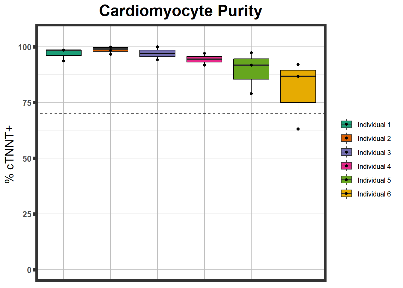
# ctnnt %>%
#   summary() %>%
#   kable(., caption= "Stats summary of cTNNT+ FACs readings") %>%
#   kable_paper("striped", full_width = FALSE) #%>%
#   kable_styling(full_width = FALSE,font_size = 18) #%>%
#   # scroll_box(width = "60%", height = "400px")
Fig. S2
drug_pal_fact <- c("#8B006D","#DF707E","#F1B72B", "#3386DD","#707031","#41B333")
library(data.table)
conf_int <- readRDS("data/plot_intv_list.RDS")
DRC_list <- readRDS("data/plot_list_DRC.RDS")
pull_drc2 <- data.frame("ind1", "ind2","ind3","ind4","ind5","ind6")
doubl_plot <- data.frame("ind3a", "ind3b", "ind5a", "ind5b")
lvl_order <- c('1','2','3','4','5','6')
intervals <- rbindlist(conf_int,idcol="trt")
drug_list <- c("DNR","DOX","EPI","MTX", "TRZ", "VEH")
# GeomRibbon$handle_na <- function(data, params) {  data }

# brewer.pal(n=6,"Dark2")
# [1] "#1B9E77" "#D95F02" "#7570B3" "#E7298A" "#66A61E" "#E6AB02"
# > display.brewer.pal(n=6,"Dark2")
for (each in 1:6){
  newdata <- intervals %>%
    separate("trt", into=c("sDrug",NA)) %>%
    dplyr::filter(sDrug ==drug_list[each]) %>%
    mutate(SampleID=indv) %>%
    mutate(indv=substr(indv,4,4)) %>%
    mutate(indv=factor(indv, levels=lvl_order)) %>%
    dplyr::filter(SampleID %in% doubl_plot)


  # newdata <- sub_intv %>%
  #  filter(indv %in% doubl_plot) %>%
  #   mutate(sub_ind=substr(indv,4,4)) %>%
  #   mutate(sub_ind=factor(sub_ind,levels=lvl_order))
  drug_plot <- DRC_list[[each]]
     f <-
       drug_plot %>%
         filter(SampleID %in% doubl_plot) %>%
         ggplot(., aes(x=Conc, y= Percent, group=SampleID,linetype=SampleID, color= indv,alpha =0.6 )) +
         guides(color="none", alpha = "none")+
         stat_smooth(method = "drm",
                     method.args = list(fct = L.4(c(NA,NA,1,NA))),
                     se = FALSE)+
         geom_ribbon(data = newdata,
                     aes(x = Conc, y = Prediction,
                         ymin = Lower,
                         ymax = Upper,
                         fill=indv),
                         alpha = 0.1,
                         color = "transparent")+
         # ylim(-.2,1.5)+
        coord_cartesian(ylim = c(-0.1, 1.5)) +
         scale_linetype_manual(values = c("dotted","solid","dotted","solid"),
                               name="replicate",
                               labels=c("Rep 1", "Rep 2","Rep 1", "Rep 2"))+
         scale_color_brewer(palette = "Dark2")+
         scale_fill_brewer(palette = "Dark2")+
         scale_x_log10() +  # Change the x-axis scale to log 10 scale
         theme_classic() +
         xlab(NULL)+
         ylab(NULL)+
        # scale_y_continuous(oob=scales::rescale_max, limits = -.4, 1.5)+
        ggtitle(drug_list[each])+
      theme(plot.title = element_text(hjust = 0.5, size =15, face ="bold"),
            axis.title=element_text(size=10),
            axis.ticks=element_line(linewidth = 2),
            axis.text=element_text(size=10, face = "bold", color="black"),
            panel.grid.major = element_line(colour = 'lightgrey'),
            panel.border=element_rect(fill = NA, linewidth = 2),
            plot.background = element_rect(fill = "white", colour = NA))

  print(f)
} 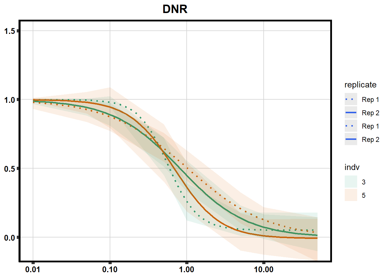
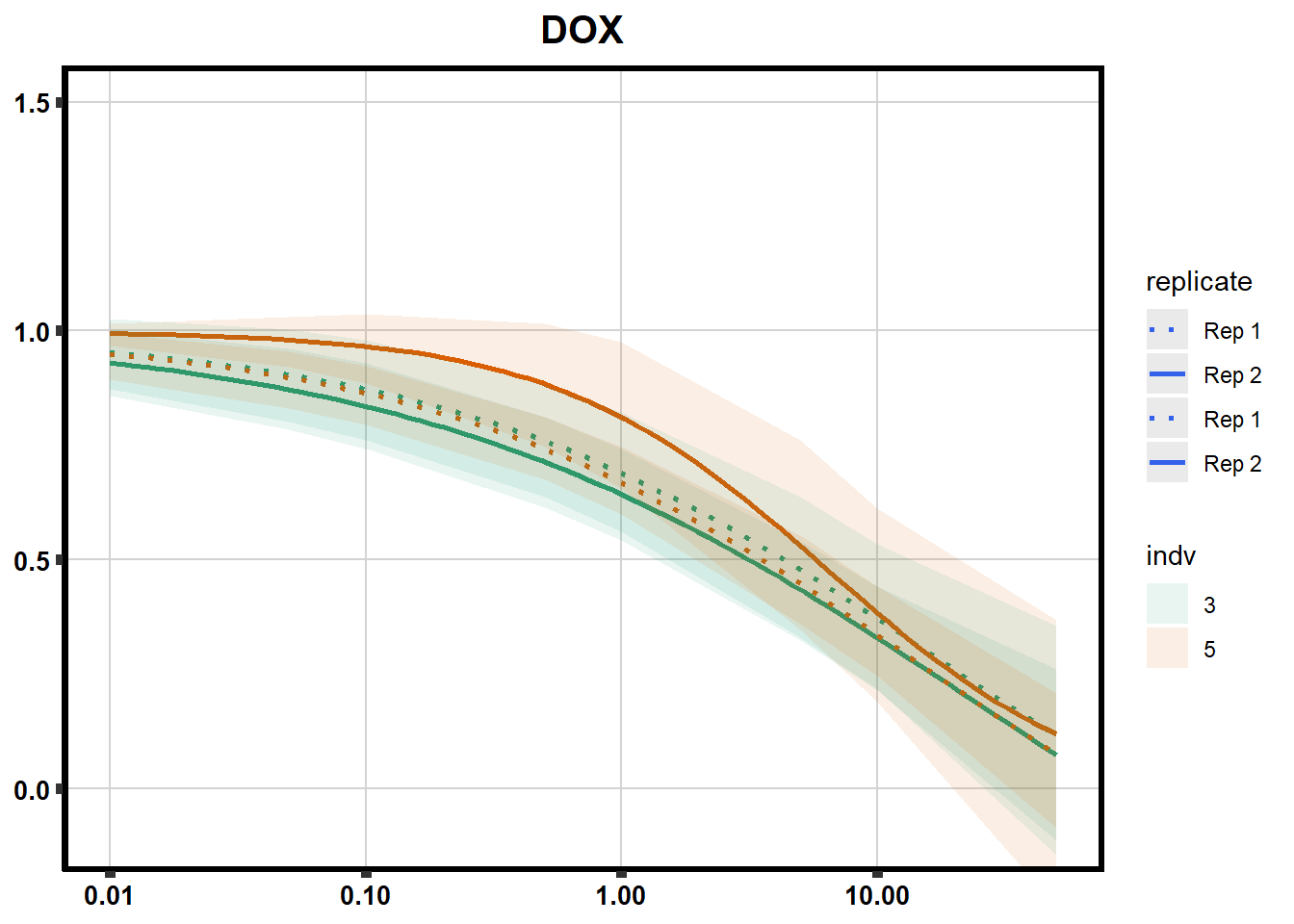
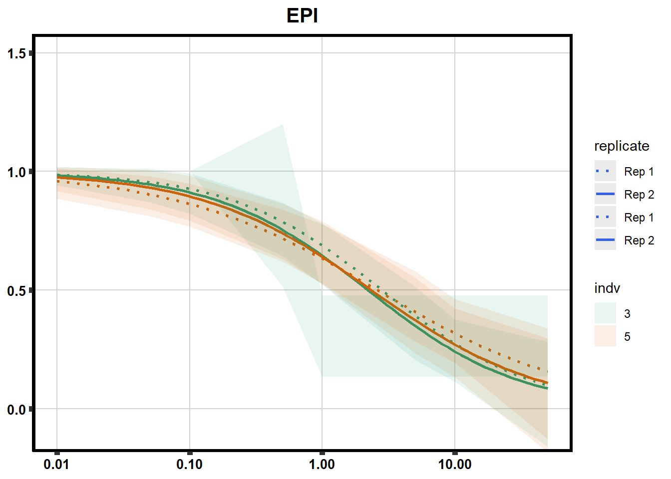
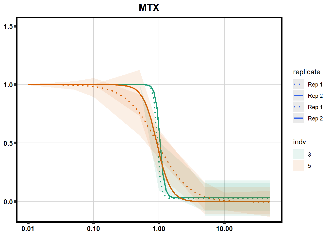
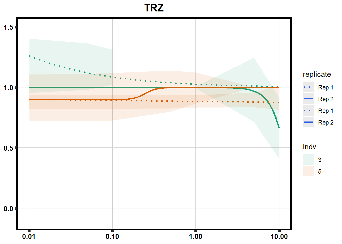
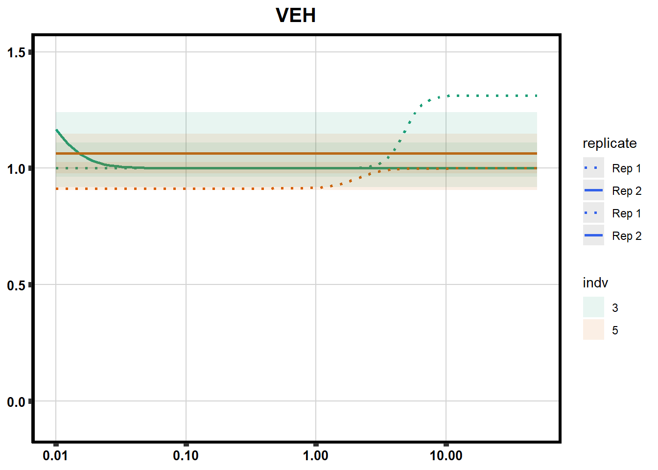
Fig. S3
viability <- readRDS("data/viability.RDS")
norm_LDH48 <- readRDS("data/supp_normLDH48.RDS")
viability %>%
  left_join(., norm_LDH48,by = c("indv","Drug","Conc")) %>%
  ggplot(., aes(x=per.live, y=ldh))+
  geom_point(aes(col=indv))+
  geom_smooth(method="lm")+
  facet_wrap(~Drug)+
  theme_bw()+
  xlab("Average viability of cardiomyocytes/100") +
  ylab("Average LDH") +
  ggtitle("Cell stress and viability correlation")+
  scale_color_brewer(palette = "Dark2",name = "Individual", label = c("1","2","3","4","5","6"))+
  ggpubr::stat_cor(method="pearson",
                   aes(label = paste(..r.label.., ..p.label.., sep = "*`,`~")),
           color = "red")+

  theme(plot.title = element_text(size = rel(1), hjust = 0.5,face = "bold"),
        axis.title = element_text(size = 12, color = "black"),
        axis.ticks = element_line(size = 1.5),
        axis.text = element_text(size = 8, color = "black", angle = 0),
        strip.text.x = element_text(size = 12, color = "black", face = "bold"),
strip.background = element_rect(fill = "transparent")) 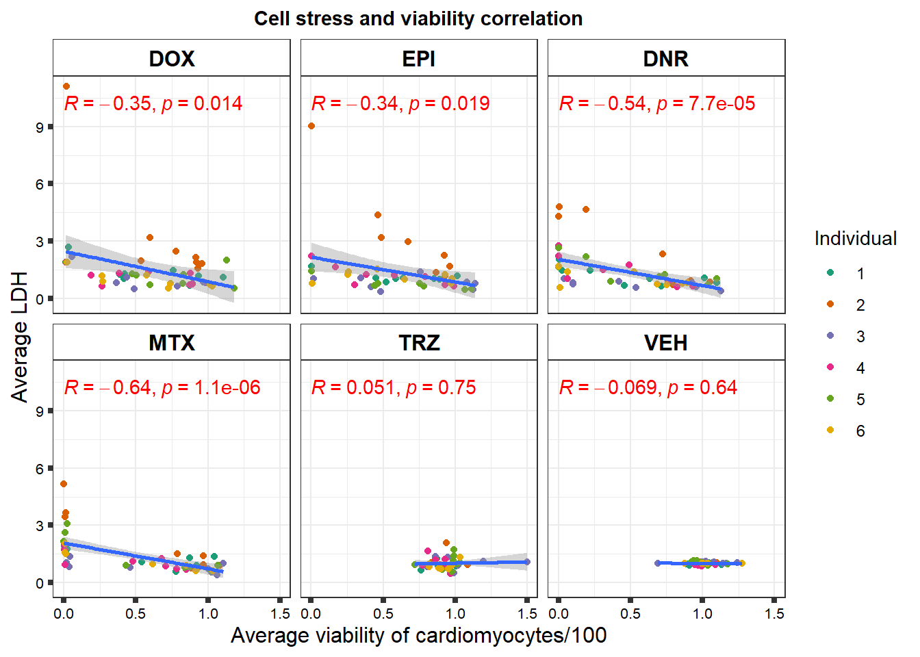
Fig. S4
viabilitytable <- readRDS("data/averageviabilitytable.RDS")


viabilitytable %>%
  ungroup() %>%
  mutate(indv=substr(SampleID,4,4)) %>%
  mutate(indv=factor(indv, levels= c('1','2','3','4','5','6'))) %>%
  dplyr::filter(Conc <5) %>%
  mutate(Conc= factor(as.numeric(Conc))) %>%
  group_by(indv,sDrug,Conc) %>%
  dplyr::summarize(Viability=mean(Mean)) %>%
  ggplot(.,  aes(x=sDrug, y= Viability*100 )) +
  geom_boxplot(position="dodge",
                 aes(fill=sDrug))+
  geom_point(aes(color=indv))+
  guides(alpha = "none")+
  ylim(0,150.5)+
  scale_color_brewer(palette = "Dark2",
                       guide="legend",
                       name ="individual",
                       labels(c(1,2,3,4,5,6)))+
  scale_fill_manual(values=drug_pal_fact, name ="treatment")+
  theme_classic() +
  xlab("")+
  ylab("% Viability") +
  facet_wrap(~Conc)+
  theme(axis.title=element_text(size=10),
        axis.ticks=element_line(size =2),
        axis.text.y=element_text(size=9, face = "bold"),
        axis.text.x=element_blank(),
        panel.grid.major = element_line(colour = 'darkgrey'),
        panel.border=element_rect(fill = NA, size = 2),
        plot.title = element_text(hjust = 0.5, size =15, face = "bold"))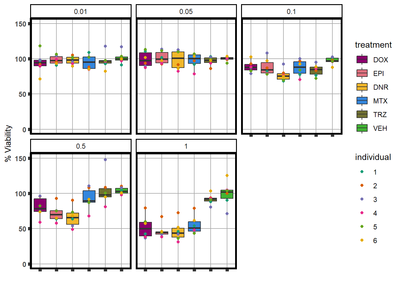
Fig. S5
library(limma)
library(edgeR)
library(cowplot)
filcpm_matrix <- readRDS("data/filcpm_counts.RDS")


x <- readRDS("data/filtermatrix_x.RDS")
x$samples %>%
  mutate(drug=case_match(drug, "Daunorubicin"~"DNR",
                        "Doxorubicin"~"DOX",
                        "Epirubicin"~"EPI",
                        "Mitoxantrone"~"MTX",
                        "Trastuzumab"~"TRZ",
                        "Vehicle"~"VEH", .default = drug)) %>%
   mutate(drug=factor(drug, levels = c('DOX','EPI','DNR','MTX','TRZ','VEH'))) %>%
  mutate(time=factor(time, labels= c("3 hours","24 hours"))) %>%
 ggplot(., aes(x = as.factor(time), y = RIN)) +
  geom_boxplot(aes(fill=as.factor(time)))+
  theme_bw()+
  ylim(c(0,10))+
  labs(x= "", fill ="Time in hours",y ="RNA Integrity Number")+
  ggtitle("Boxplot of RIN by time and drug")+
  facet_wrap(~drug)+
  theme(plot.title = element_text(size = rel(1.5), hjust = 0.5),
        axis.title = element_text(size = 15, color = "black"),
        axis.text.y = element_text(size =10, color = "black", angle = 0, hjust = 0.8, vjust = 0.5),
        axis.text.x = element_text(size =10, color = "black", angle = 0, hjust = 1, vjust = 0.2),
        strip.text.x = element_text(size = 15, color = "black", face = "bold"),
        strip.background = element_rect(fill = "white"))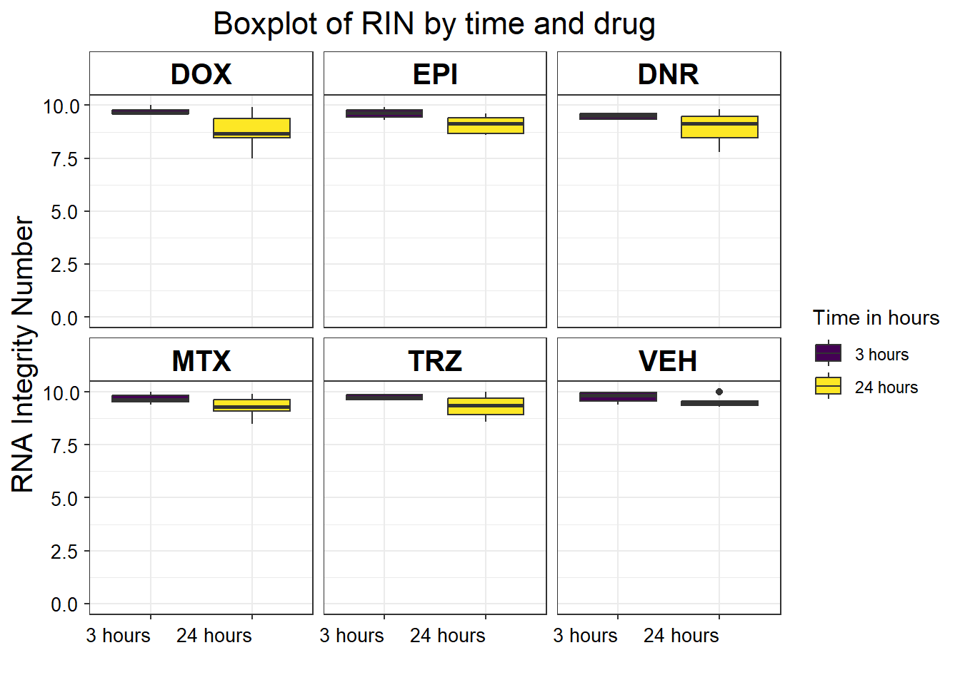
seq_info <-read.csv("output/sequencing_info.txt", row.names = 1)
seq_info %>%

  filter(type=="Total_reads") %>%
  mutate(drug=case_match(drug, "Daunorubicin"~"DNR",
                        "Doxorubicin"~"DOX",
                        "Epirubicin"~"EPI",
                        "Mitoxantrone"~"MTX",
                        "Trastuzumab"~"TRZ",
                        "Vehicle"~"VEH", .default = drug)) %>%
   mutate(drug=factor(drug, levels = c('DOX','EPI','DNR','MTX','TRZ','VEH'))) %>%
    ggplot(., aes (x =drug, y=Total.Sequences, fill = drug))+
  geom_boxplot()+
  scale_fill_manual(values=drug_pal_fact)+
  ggtitle(expression("Total number of reads by treatment"))+
  xlab(" ")+
  ylab(expression("RNA -sequencing reads"))+
  theme_bw()+
  theme(plot.title = element_text(size = rel(1.5), hjust = 0.5),
        axis.title = element_text(size = 12, color = "black"),
        axis.ticks = element_line(linewidth = 1.5),
        axis.line = element_line(linewidth = 1.5),
        axis.text.y = element_text(size =10, color = "black", angle = 0, hjust = 0.8, vjust = 0.5),
        axis.text.x = element_text(size =10, color = "white"),
        #strip.text.x = element_text(size = 15, color = "black", face = "bold"),
        strip.text.y = element_text(color = "white"))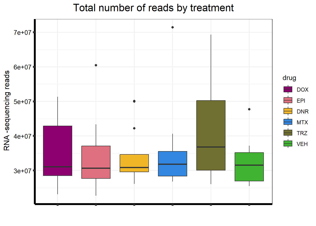
seq_info %>%
mutate(drug=case_match(drug, "Daunorubicin"~"DNR",
"Doxorubicin"~"DOX",
"Epirubicin"~"EPI",
"Mitoxantrone"~"MTX",
"Trastuzumab"~"TRZ",
"Vehicle"~"VEH", .default = drug)) %>%
mutate(drug=factor(drug, levels = c('DOX','EPI','DNR','MTX','TRZ','VEH'))) %>%
# separate(samplenames, into=c(NA,NA,NA,"samplenames")) %>%
# mutate(shortnames = paste("Sample",str_trim(samplenames))) %>%
filter(type=="Total_reads") %>%
mutate(sampleID=colnames(filcpm_matrix)) %>%
ggplot(., aes (x =sampleID, y=Total.Sequences, fill = drug, group_by=indv))+
geom_col()+
geom_hline(aes(yintercept=20000000))+
scale_fill_manual(values=drug_pal_fact)+
ggtitle(expression("Total number of reads by sample"))+
xlab("")+
ylab(expression("RNA -sequencing reads"))+
theme_bw()+
theme(plot.title = element_text(size = rel(2), hjust = 0.5),
axis.title = element_text(size = 15, color = "black"),
axis.ticks = element_line(linewidth = 1.5),
axis.line = element_line(linewidth = 1.5),
axis.text.y = element_text(size =10, color = "black", angle = 0, hjust = 0.8, vjust = 0.5),
axis.text.x = element_text(size =6, color = "black", angle = 90, hjust = 1, vjust = 0.2),
#strip.text.x = element_text(size = 15, color = "black", face = "bold"),
strip.text.y = element_text(color = "white"))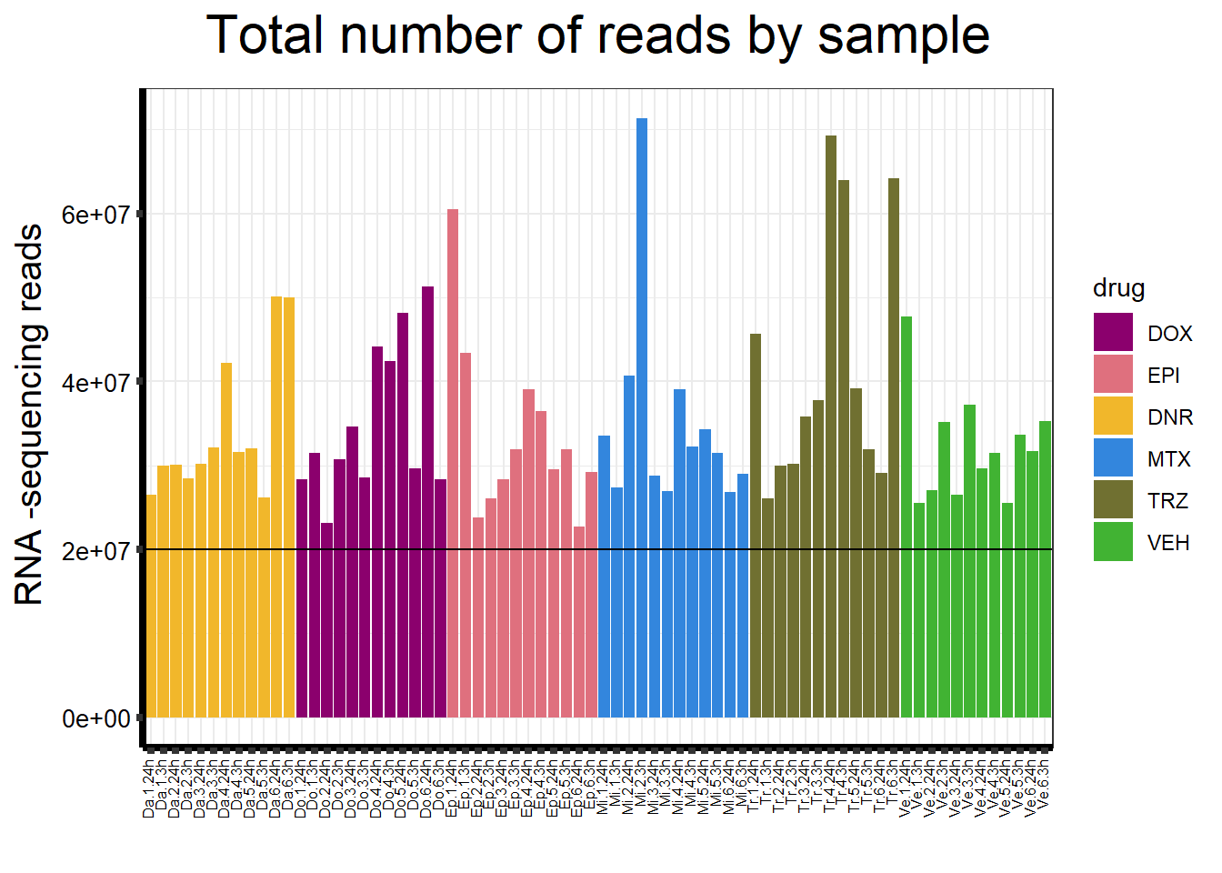 ### Fig. S6
filcpm_matrix <- readRDS("data/filcpm_counts.RDS")

mcor <- cor(filcpm_matrix)

filmat_groupmat_col <- data.frame(timeset = colnames(filcpm_matrix))
counts_corr_mat<- filmat_groupmat_col %>%
  separate(timeset, into= c("drug","indv","time")) %>%
  mutate(class = if_else(drug=="Da","AC", if_else(drug=="Do","AC", if_else(drug=="Ep","AC","nAC")))) %>%
  mutate(TOP2i = if_else(drug=="Da","yes", if_else(drug=="Do","yes", if_else(drug=="Ep","yes",if_else(drug=="Mi","yes","no")))))

 mat_colors <- list(
   drug= c("#F1B72B","#8B006D","#DF707E","#3386DD","#707031","#41B333"),
   indv=c("#1B9E77", "#D95F02" ,"#7570B3", "#E7298A" ,"#66A61E", "#E6AB02"),
   time=c("pink", "chocolate4"),
   class=c("yellow1","lightgreen"),
   TOP2i =c("darkgreen","goldenrod"))

names(mat_colors$drug)   <- unique(counts_corr_mat$drug)
names(mat_colors$indv) <- unique(counts_corr_mat$indv)
names(mat_colors$time) <- unique(counts_corr_mat$time)
names(mat_colors$class) <- unique(counts_corr_mat$class)
names(mat_colors$TOP2i) <- unique(counts_corr_mat$TOP2i)


ComplexHeatmap::pheatmap(mcor,
                         # column_title=(paste0("RNA-seq log"[2]~"cpm correlation")),
        annotation_col = counts_corr_mat,
        annotation_colors = mat_colors,
                         fontsize=10,
                         fontsize_row = 8,
                         angle_col="90",
                         treeheight_row=25,
                         fontsize_col = 8,
                         treeheight_col = 20)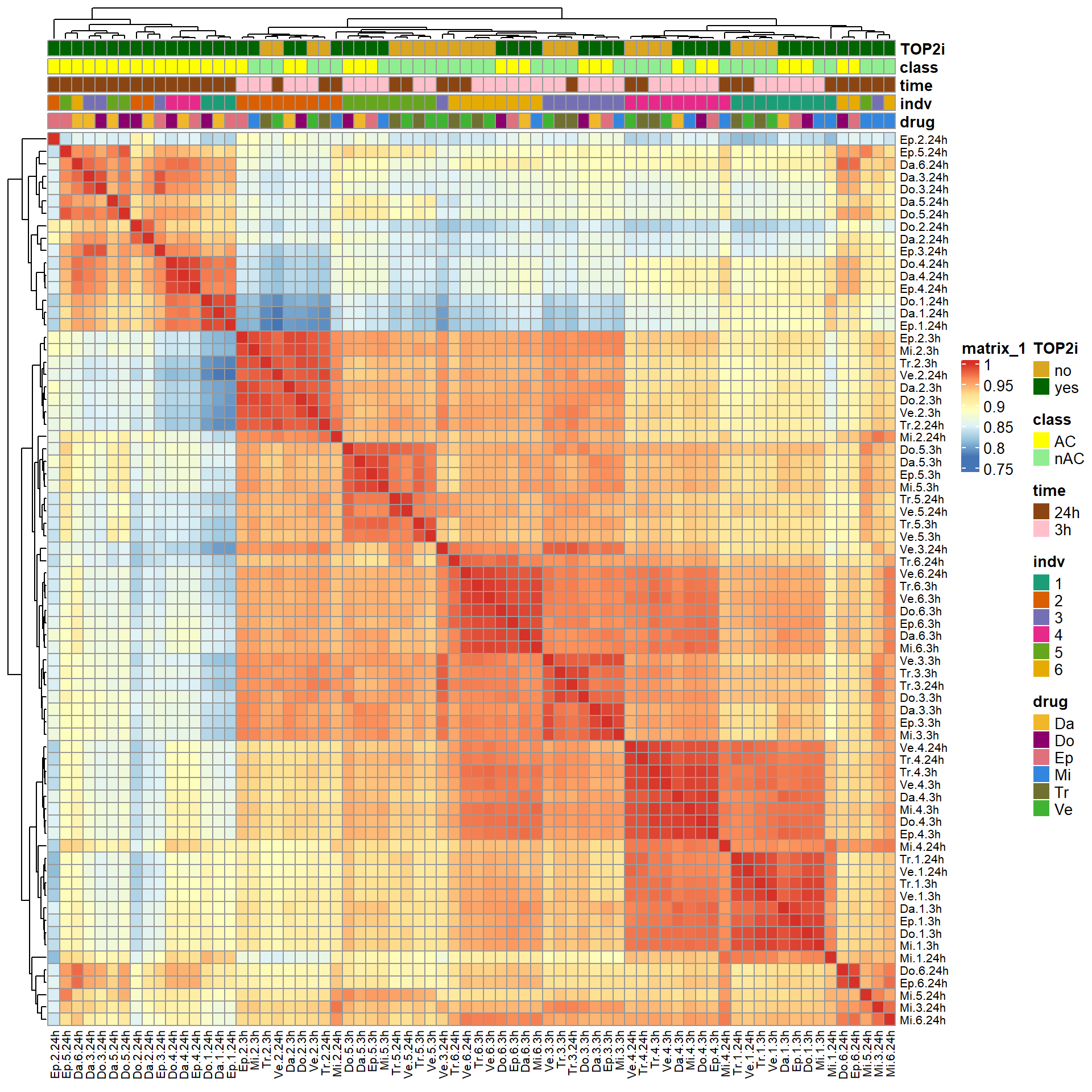
Fig. S7
pca_all_anno <- readRDS("data/supp_pca_all_anno.RDS")
pca_all_anno <- pca_all_anno %>%
  mutate(drug = case_match(drug, "Daunorubicin"~"DNR","Doxorubicin"~"DOX", "Epirubicin"~"EPI","Mitoxantrone"~"MTX","Trastuzumab"~"TRX","Vehicle"~"VEH", .default = drug))


facs <- c("indv", "drug", "time")
names(facs) <- c("Individual", "Treatment", "Time")

get_regr_pval <- function(mod) {
  # Returns the p-value for the Fstatistic of a linear model
  # mod: class lm
  stopifnot(class(mod) == "lm")
  fstat <- summary(mod)$fstatistic
  pval <- 1 - pf(fstat[1], fstat[2], fstat[3])
  return(pval)
}

plot_versus_pc <- function(df, pc_num, fac) {
  # df: data.frame
  # pc_num: numeric, specific PC for plotting
  # fac: column name of df for plotting against PC
  pc_char <- paste0("PC", pc_num)
  # Calculate F-statistic p-value for linear model
  pval <- get_regr_pval(lm(df[, pc_char] ~ df[, fac]))
  if (is.numeric(df[, f])) {
    ggplot(df, aes_string(x = f, y = pc_char)) + geom_point() +
      geom_smooth(method = "lm") + labs(title = sprintf("p-val: %.2f", pval))
  } else {
    ggplot(df, aes_string(x = f, y = pc_char)) + geom_boxplot() +
      labs(title = sprintf("p-val: %.2f", pval))
  }
}

for (f in facs) {
    # Plot f versus PC1 and PC2
  f_v_pc1 <- arrangeGrob(plot_versus_pc(pca_all_anno, 1, f)+theme_bw())
  f_v_pc2 <- arrangeGrob(plot_versus_pc(pca_all_anno, 2, f)+theme_bw())
  grid.arrange(f_v_pc1, f_v_pc2, ncol = 2, top = names(facs)[which(facs == f)])
}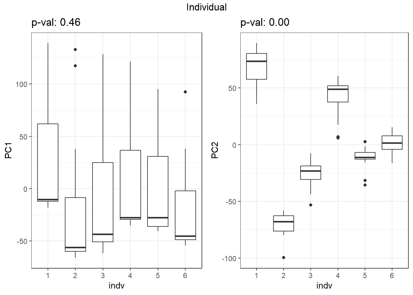
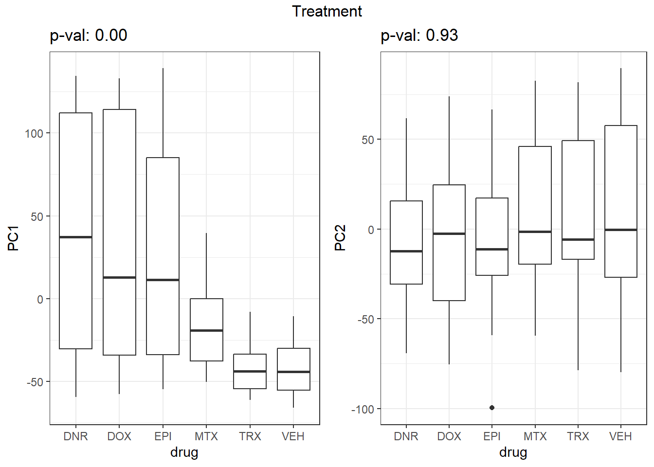
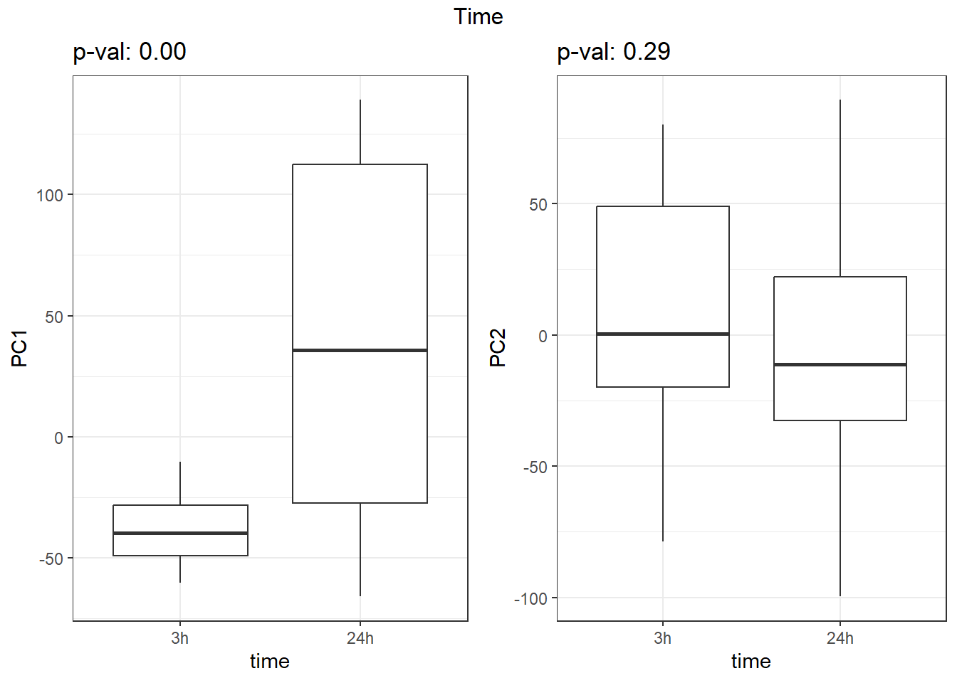
Fig. S8
Volcanoplots <- readRDS("output/Volcanoplot_10.RDS")
Volcanoplots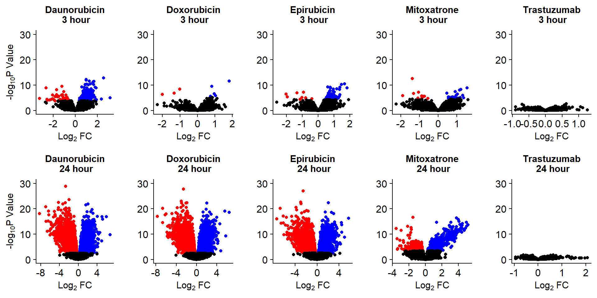
Fig. S9
toplistall <- readRDS("data/toplistall.RDS")
toplistall %>%
  group_by(time, id) %>%
  mutate(id=factor(id, levels = c('DOX', 'EPI', 'DNR', 'MTX', 'TRZ','VEH'))) %>%
  mutate(time= factor(time,
     levels=c("3_hours","24_hours"),
              labels=c("3 hours","24 hours"))) %>%
  ggplot(., aes(x=id, y=logFC))+
  geom_boxplot(aes(fill=id))+
  ggpubr::fill_palette(palette =drug_pal_fact)+
  guides(fill=guide_legend(title = "Treatment"))+
  # facet_wrap(sigcount~time)+
  theme_bw()+
  xlab("")+
  ylab(expression("Log"[2]*" fold change"))+
  theme_bw()+
  facet_wrap(~time)+
  theme(plot.title = element_text(size = rel(1.5), hjust = 0.5),
        axis.title = element_text(size = 15, color = "black"),
        # axis.ticks = element_line(linewidth = 1.5),
        # axis.line = element_line(linewidth = 1.5),
        strip.background = element_rect(fill = "transparent"),
        axis.text.x = element_blank(),
        strip.text.x = element_text(size = 12, color = "black", face = "bold"))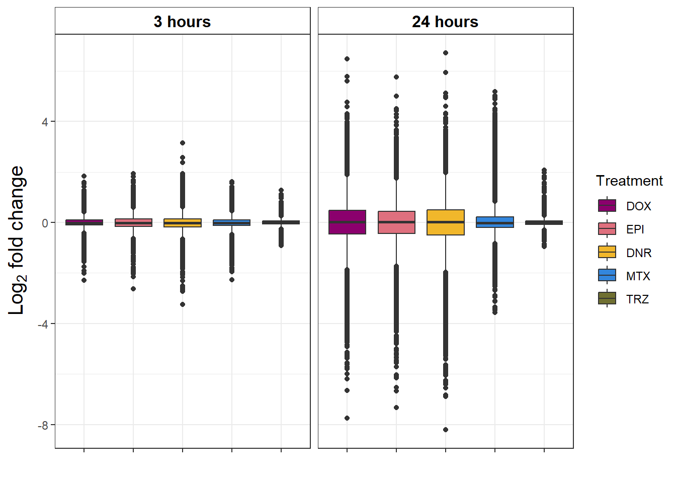
# drug_palNoVeh <- c("#8B006D" ,"#DF707E", "#F1B72B" ,"#3386DD", "#707031")

ggsave("output/Figures/Percent_DEG-1.eps",width = 6, height =4, units = "in")
toplistall %>%
    mutate(id=factor(id, levels = c('DOX', 'EPI', 'DNR', 'MTX', 'TRZ','VEH'))) %>%
  mutate(time= factor(time,
     levels=c("3_hours","24_hours"),
              labels=c("3 hours","24 hours"))) %>%
  group_by(time, id) %>%
  mutate(sigcount = if_else(adj.P.Val < 0.05,'sig','notsig'))%>%
  count(sigcount) %>%
  pivot_wider(id_cols = c(time,id), names_from=sigcount, values_from=n) %>%
  mutate(prop = sig/(sig+notsig)*100) %>%
  mutate(prop=if_else(is.na(prop),0,prop)) %>%
  ggplot(., aes(x=id, y= prop))+
  geom_col(aes(fill=id))+
  geom_text(aes(label = sprintf("%.2f",prop)),
            position=position_dodge(0.9),vjust=-.2 )+
  scale_fill_manual(values =drug_pal_fact)+
  guides(fill=guide_legend(title = "Treatment"))+
  facet_wrap(~time)+#labeller = (time = facettimelabel) )+
  theme_bw()+
  xlab("")+
  ylab("Percentage of expressed genes")+
  theme_bw()+
  ggtitle("Percent DEGs (adj. P value <0.05)")+
  scale_y_continuous(expand=expansion(c(0.02,.2)))+
  theme(plot.title = element_text(size = rel(1.5), hjust = 0.5),
        axis.title = element_text(size = 15, color = "black"),
        # axis.ticks = element_line(linewidth = 1.5),
        # axis.line = element_line(linewidth = 1.5),
        strip.background = element_rect(fill = "transparent"),
        axis.text.x = element_text(size = 8, color = "white", angle = 0),
        axis.text.y = element_text(size = 8, color = "black", angle = 0),
        strip.text.x = element_text(size = 12, color = "black", face = "bold"))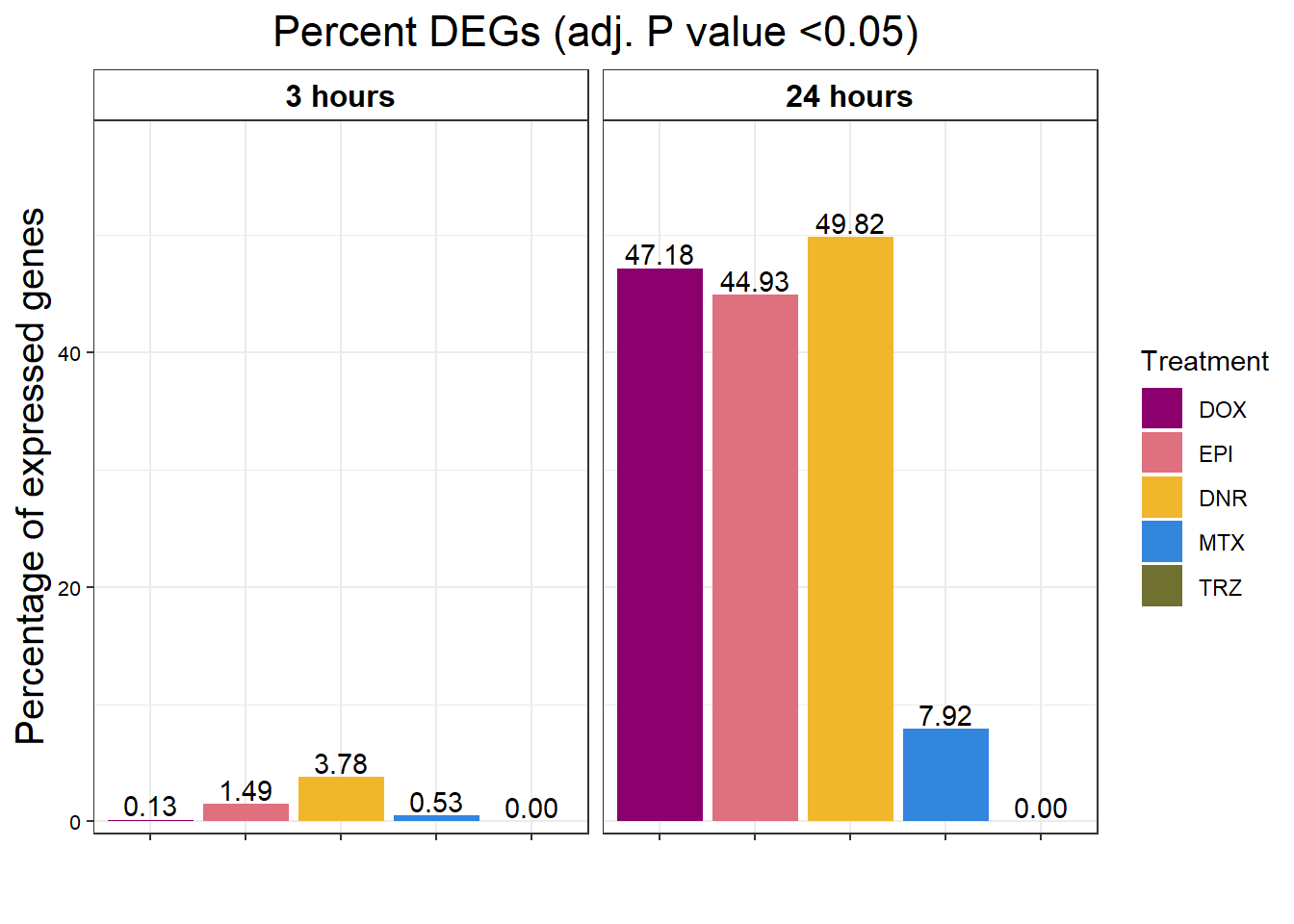
ggsave("output/Figures/Percent_DEG-2.eps",width = 6, height =4, units = "in")Fig. S10
Fig S10 Drug Specific Pathways
gostres3Dnrdeg_sp <- readRDS("data/DEG-GO/gostres3Dnrdeg_sp.RDS")

Dnr3_sp_DEGtable <- gostres3Dnrdeg_sp$result %>%
  dplyr::select(c(source, term_id,term_name,intersection_size,
                   term_size, p_value))


Dnr3_sp_DEGtable  %>%
    dplyr::filter(source=="GO:BP") %>%
    dplyr::select(p_value,term_name,intersection_size) %>%
    slice_min(., n=10 ,order_by=p_value) %>%
    mutate(log_val = -log10(p_value)) %>%
   # slice_max(., n=10,order_by = p_value) %>%
   ggplot(., aes(x = log_val, y =reorder(term_name,p_value), col= intersection_size)) +
    geom_point(aes(size = intersection_size)) +
    scale_y_discrete(labels =scales::label_wrap(30))+
    guides(col="none", size=guide_legend(title = "# of intersected \n terms"))+
    ggtitle('DNR 3 hour specific(stringent)\n gene set GO:BP terms') +
    xlab(expression(" -"~log[10]~("adj. p-value")))+
    ylab("GO: BP term")+
    theme_bw()+
    theme(plot.title = element_text(size = rel(1.5), hjust = 0.5),
        axis.title = element_text(size = 15, color = "black"),
        axis.ticks = element_line(linewidth = 1.5),
        axis.line = element_line(linewidth = 1.5),
        axis.text = element_text(size = 10, color = "black", angle = 0),
        strip.text.x = element_text(size = 12, color = "black", face = "bold"))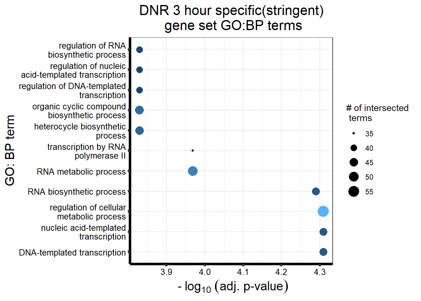
gostres3Mtxdeg_sp <- readRDS("data/DEG-GO/gostres3Mtxdeg_sp.RDS")
Mtx3_sp_DEGtable <- gostres3Mtxdeg_sp$result %>%
  dplyr::select(c(source, term_id,term_name,intersection_size,
                   term_size, p_value))
Mtx3_sp_DEGtable  %>%
    dplyr::filter(source=="GO:BP") %>%
    dplyr::select(p_value,term_name,intersection_size) %>%
    slice_min(., n=5,order_by=p_value) %>%
    mutate(log_val = -log10(p_value)) %>%
   # slice_max(., n=10,order_by = p_value) %>%
   ggplot(., aes(x = log_val, y =reorder(term_name,p_value), col= intersection_size)) +
    geom_point(aes(size = intersection_size)) +
    scale_y_discrete(labels = scales::label_wrap(30))+
  geom_vline(xintercept = (-log10(0.05)))+
    guides(col="none", size=guide_legend(title = "# of intersected \n terms"))+
    ggtitle('MTX 3 hour specific(stringent)\n gene set GO:BP terms') +
    xlab(expression(" -"~log[10]~("adj. p-value")))+
    ylab("GO: BP term")+
    theme_bw()+
    theme(plot.title = element_text(size = rel(1.5), hjust = 0.5),
        axis.title = element_text(size = 15, color = "black"),
        axis.ticks = element_line(linewidth = 1.5),
        axis.line = element_line(linewidth = 1.5),
        axis.text = element_text(size = 10, color = "black", angle = 0),
        strip.text.x = element_text(size = 12, color = "black", face = "bold"))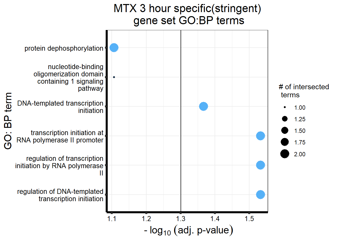
DX_sp_DEGgostres <- readRDS("data/DEG-GO/gostresDOXdeg_sp.RDS")
MT_sp_DEGgostres <- readRDS("data/DEG-GO/gostresMTXdeg_sp.RDS")

DX_sp_DEGtable <- DX_sp_DEGgostres$result %>%
  dplyr::select(c(source, term_id,term_name,intersection_size,
                   term_size, p_value))
MT_sp_DEGtable <- MT_sp_DEGgostres$result %>%
  dplyr::select(c(source, term_id,term_name,intersection_size,
                   term_size, p_value))


DX_sp_DEGtable  %>%
    dplyr::filter(source=="GO:BP") %>%
    dplyr::select(p_value,term_name,intersection_size) %>%
    slice_min(., n=10 ,order_by=p_value) %>%
    mutate(log_val = -log10(p_value)) %>%
   # slice_max(., n=10,order_by = p_value) %>%
   ggplot(., aes(x = log_val, y =reorder(term_name,p_value), col= intersection_size)) +
    geom_point(aes(size = intersection_size)) +
    scale_y_discrete(labels = scales::wrap_format(30))+
    guides(col="none", size=guide_legend(title = "# of intersected \n terms"))+
    ggtitle('DOX specific 24 hour gene set GO:BP terms') +
    xlab(expression(" -"~log[10]~("adj. p-value")))+
    ylab("GO: BP term")+
    theme_bw()+
    theme(plot.title = element_text(size = rel(1.5), hjust = 0.5),
        axis.title = element_text(size = 15, color = "black"),
        axis.ticks = element_line(linewidth = 1.5),
        axis.line = element_line(linewidth = 1.5),
        axis.text = element_text(size = 10, color = "black", angle = 0),
        strip.text.x = element_text(size = 12, color = "black", face = "bold"))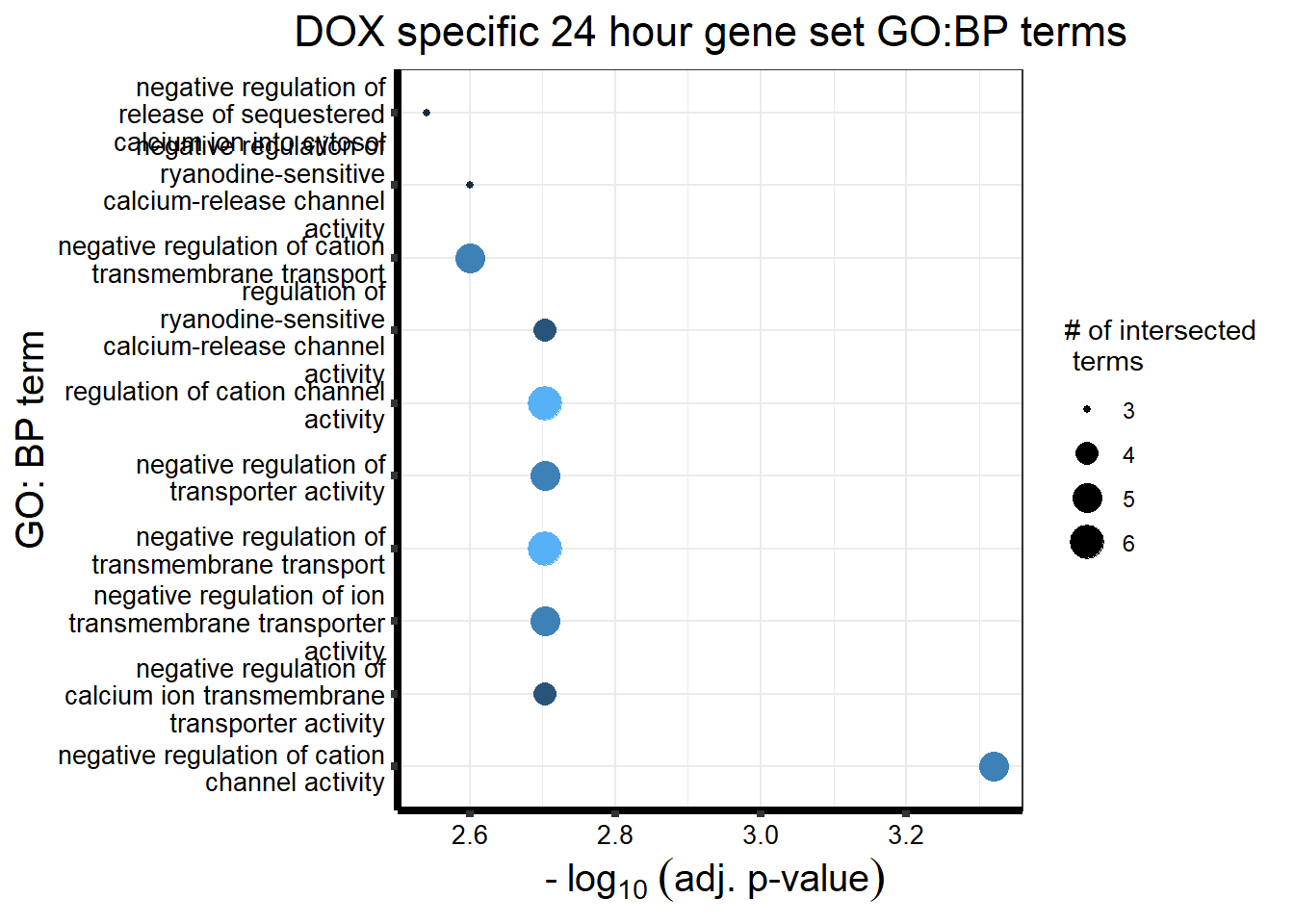
MT_sp_DEGtable  %>%
    dplyr::filter(source=="GO:BP") %>%
    dplyr::select(p_value,term_name,intersection_size) %>%
    slice_min(., n=10 ,order_by=p_value) %>%
    mutate(log_val = -log10(p_value)) %>%
   # slice_max(., n=10,order_by = p_value) %>%
   ggplot(., aes(x = log_val, y =reorder(term_name,p_value), col= intersection_size)) +
    geom_point(aes(size = intersection_size)) +
    scale_y_discrete(labels = scales::wrap_format(30))+
    guides(col="none", size=guide_legend(title = "# of intersected \n terms"))+
    ggtitle('MTX specific 24 hour gene set GO:BP terms') +
    xlab(expression(" -"~log[10]~("adj. p-value")))+
    ylab("GO: BP term")+
    theme_bw()+
    theme(plot.title = element_text(size = rel(1.5), hjust = 0.5),
        axis.title = element_text(size = 15, color = "black"),
        axis.ticks = element_line(linewidth = 1.5),
        axis.line = element_line(linewidth = 1.5),
        axis.text = element_text(size = 10, color = "black", angle = 0),
        strip.text.x = element_text(size = 12, color = "black", face = "bold"))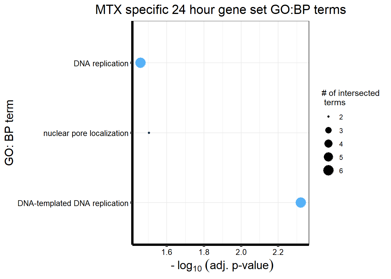
Fig. S12
DNRvenn<- readRDS ("output/DNRvenn.RDS")
DOXvenn<- readRDS ("output/DOXvenn.RDS")
EPIvenn<- readRDS ("output/EPIvenn.RDS")
MTXvenn<- readRDS ("output/MTXvenn.RDS")

plot_grid(DNRvenn,DOXvenn,EPIvenn,MTXvenn,nrow=2, ncol = 2)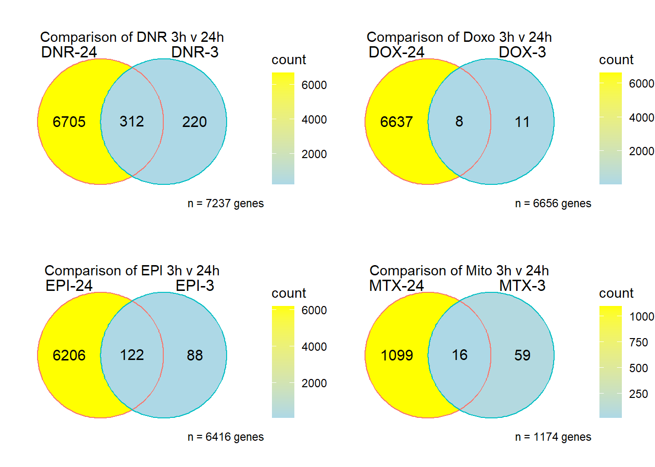
Fig. S12
motif_NRrep <-  readRDS("output/motif_NRrep.RDS")
motif_ERrep <-  readRDS("output/motif_ERrep.RDS")
motif_TIrep <-  readRDS("output/motif_TI_rep.RDS")
motif_LRrep <-  readRDS("output/motif_LRrep.RDS")
motif_NRrep <- motif_NRrep +
  scale_y_continuous(labels = scales::number_format(accuracy = 0.1))+
  theme(legend.position = "NULL", axis.title.y =element_text(size =12))

motif_ERrep <- motif_ERrep+
  scale_y_continuous(labels = scales::number_format(accuracy = 0.1))+
  theme(legend.position = "NULL", axis.title.y =element_text(size =12))

motif_TIrep <- motif_TIrep+
  scale_y_continuous(labels = scales::number_format(accuracy = 0.1))+
  theme(legend.position = "NULL", axis.title.y =element_text(size =12))

motif_LRrep <- motif_LRrep+
  scale_y_continuous(labels = scales::number_format(accuracy = 0.1))+
  theme(legend.position = "NULL", axis.title.y =element_text(size =12))
plot_grid(motif_ERrep,motif_TIrep,motif_LRrep,motif_NRrep,nrow = 4,ncol = 1)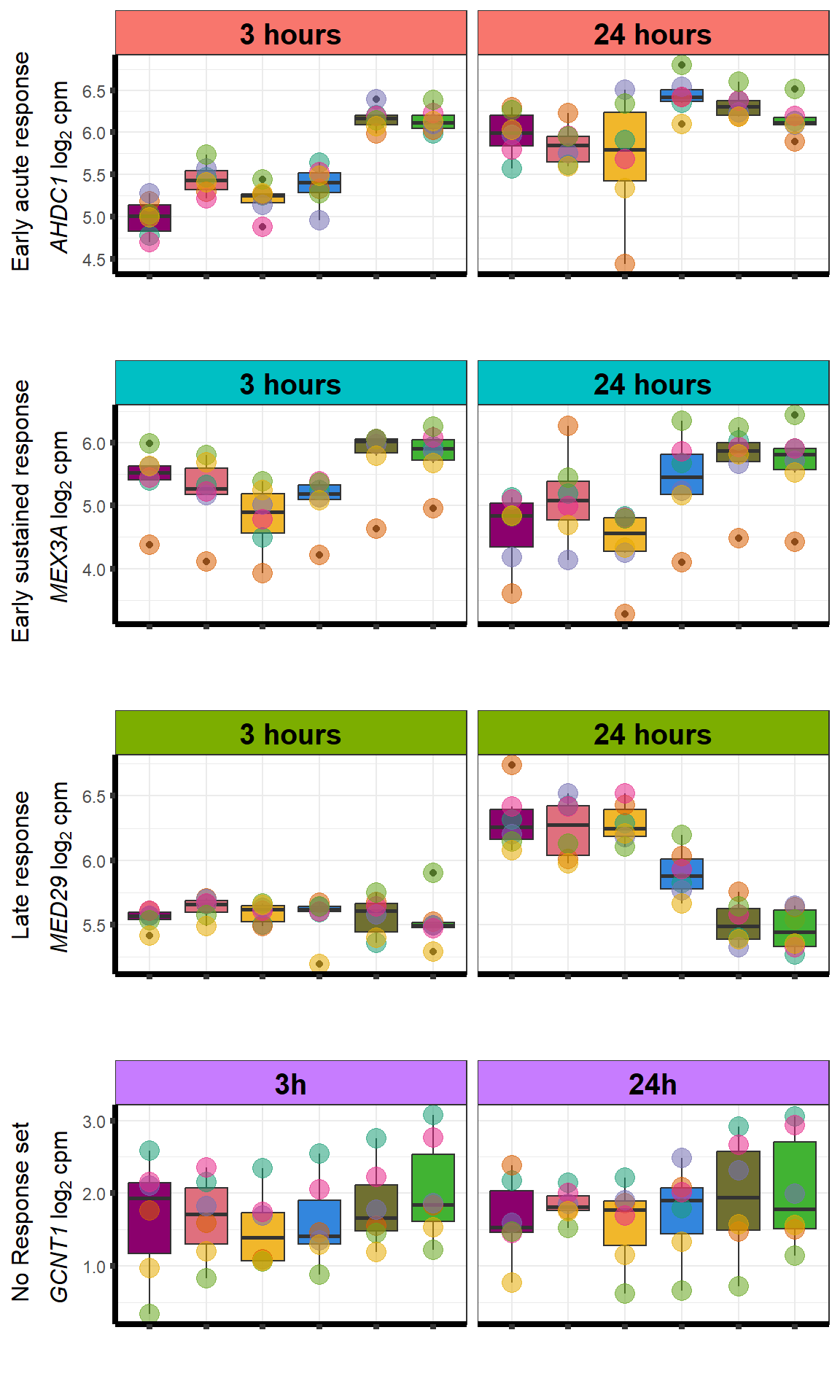
<environment: R_GlobalEnv>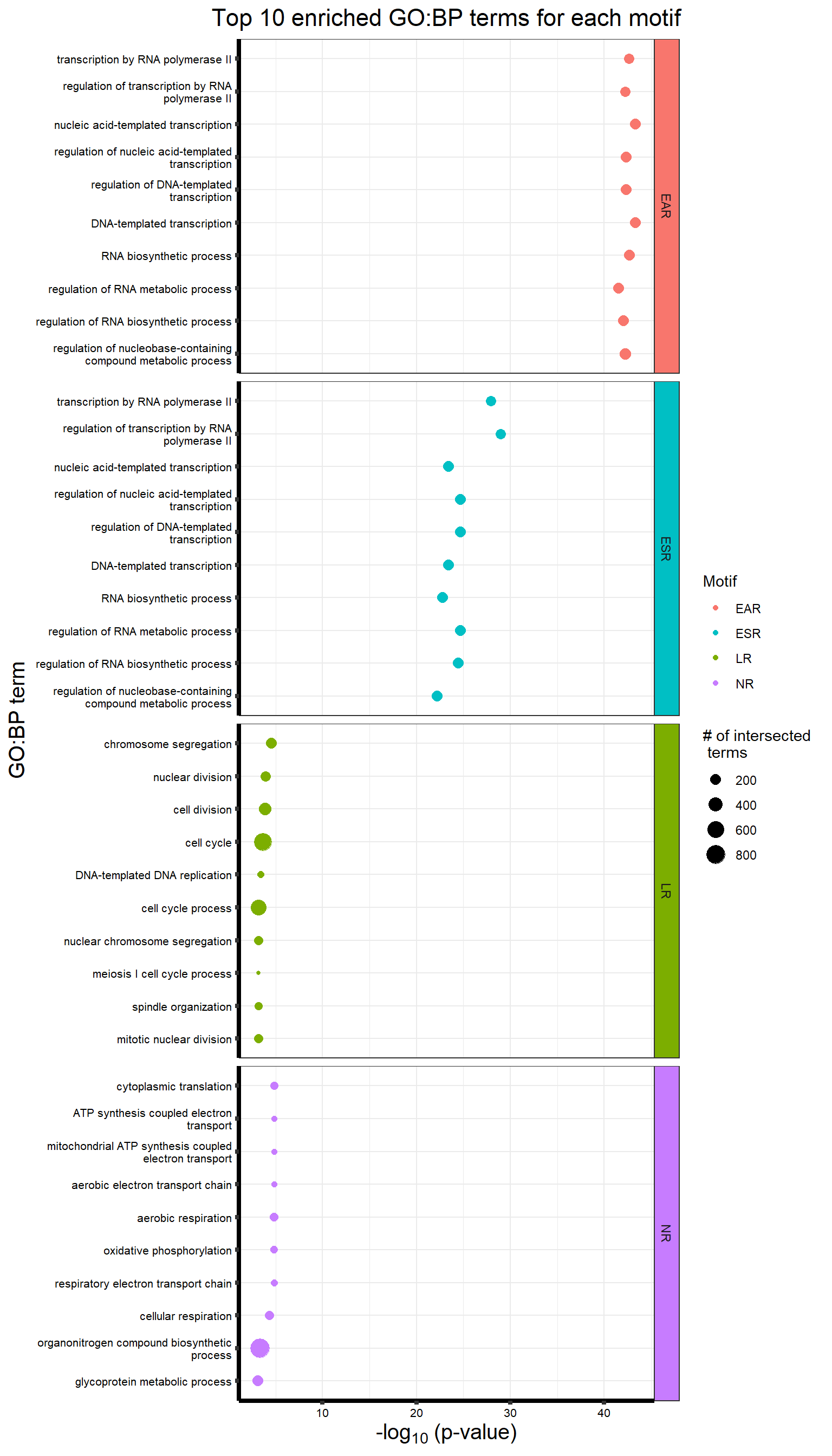
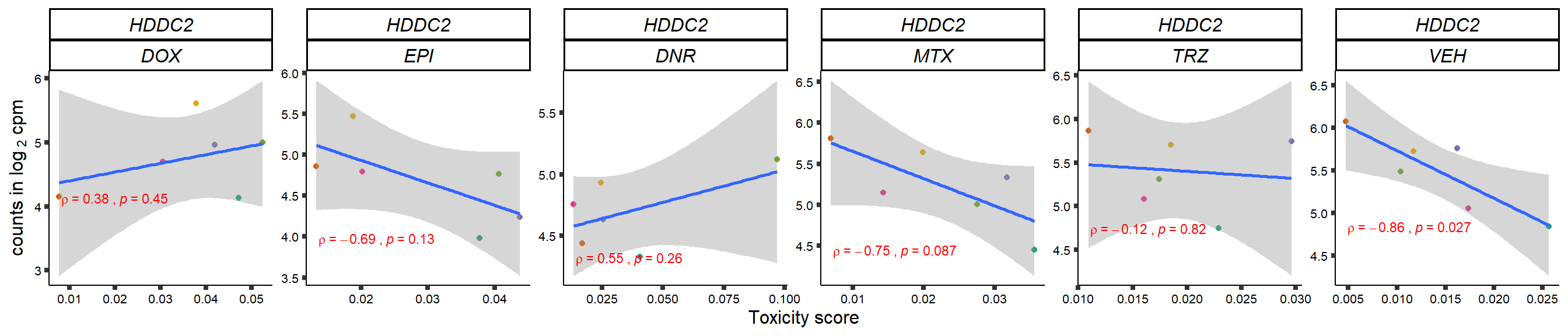
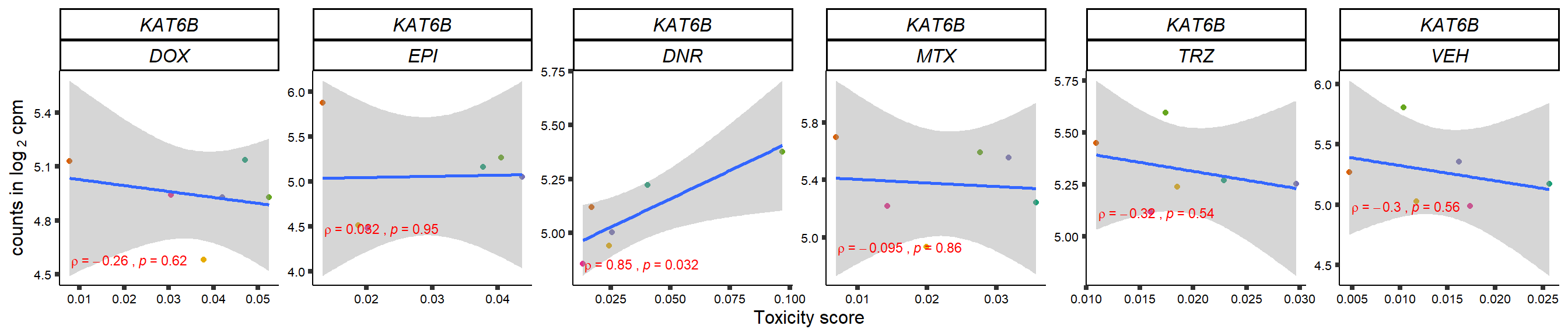
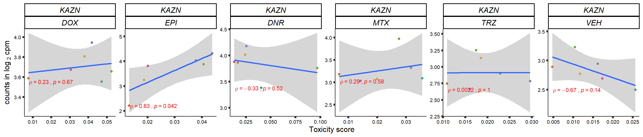
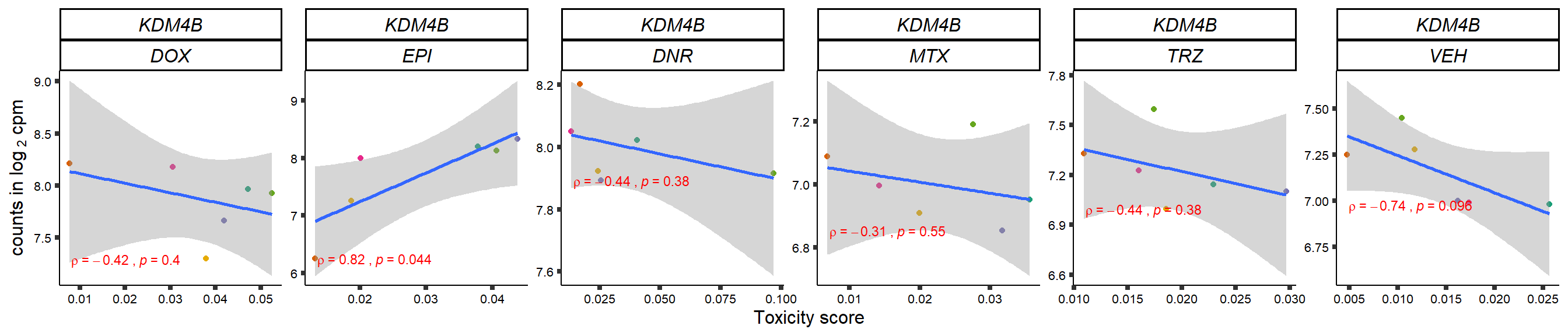
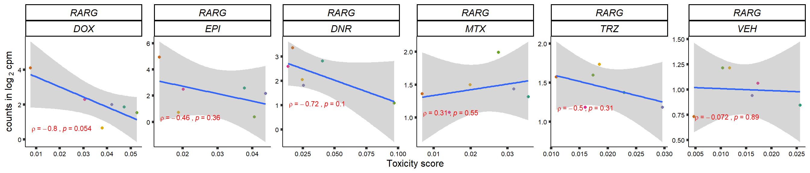
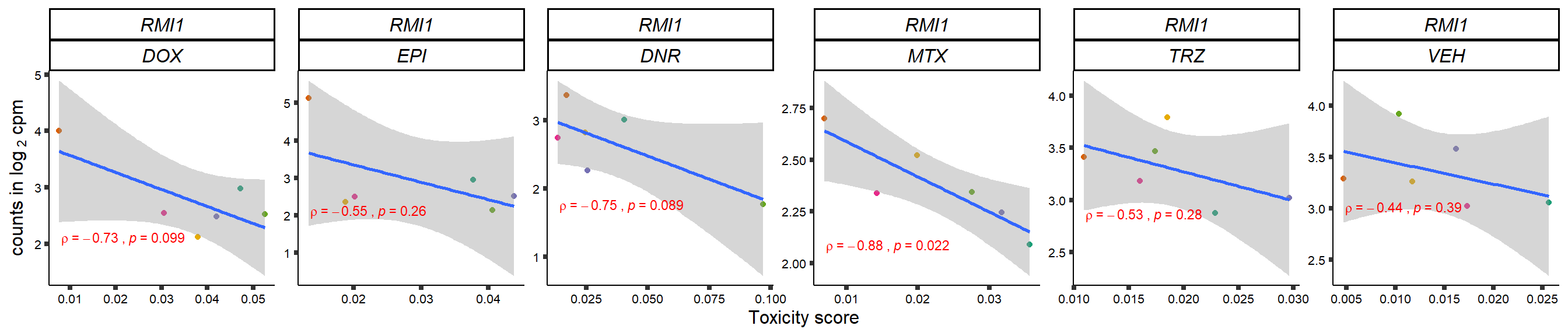
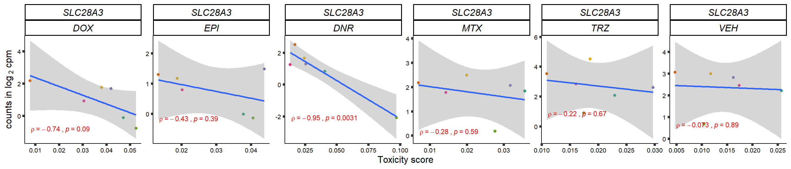
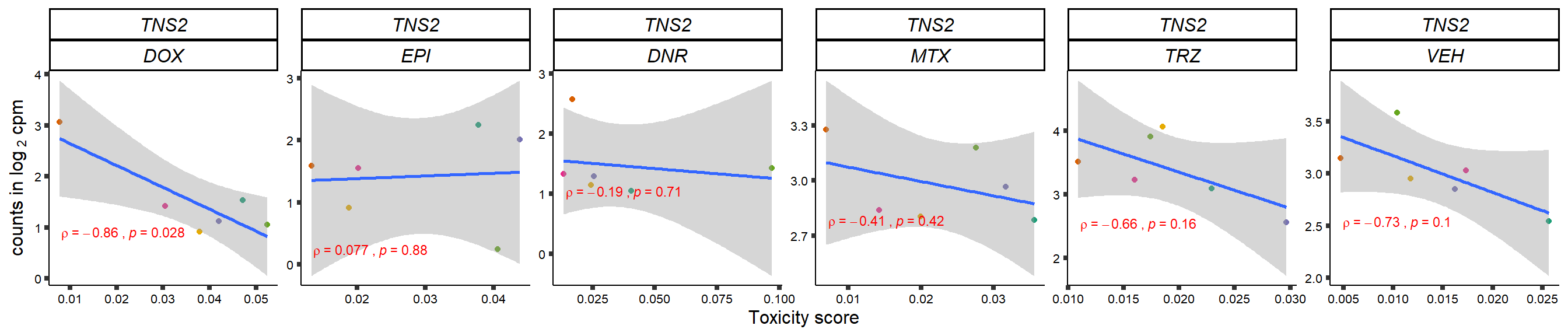
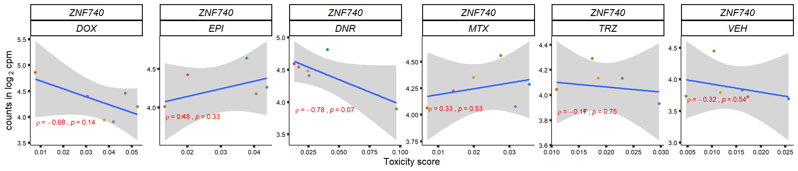
Fig. S15
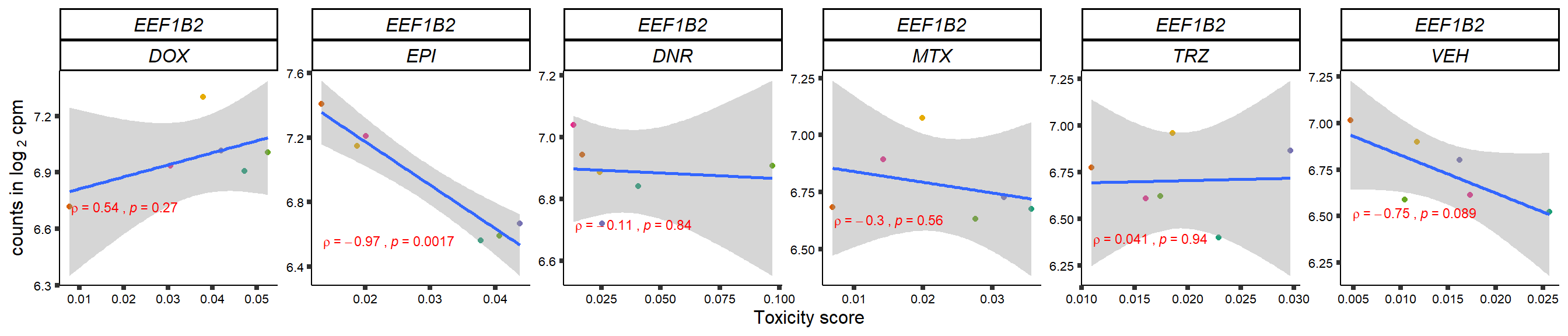
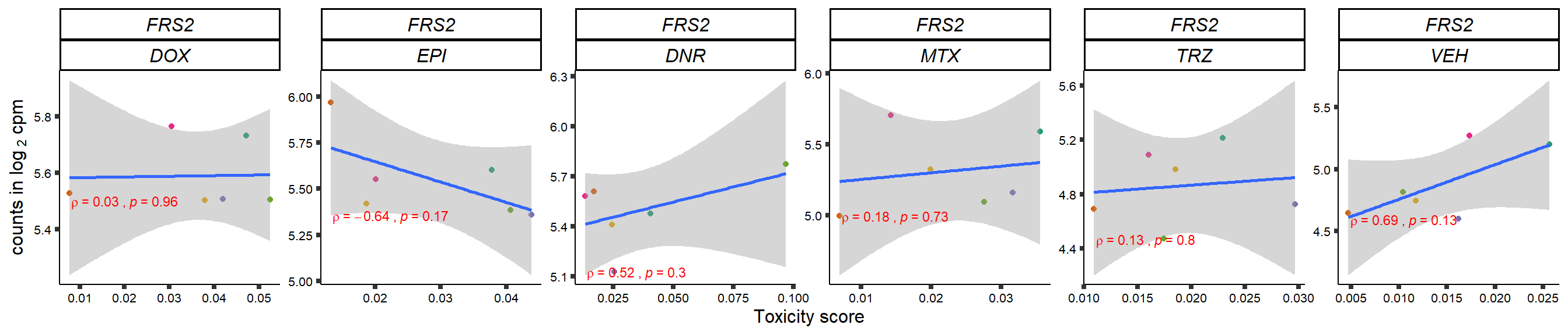
gene_corr_frame <- readRDS("data/gene_corr_frame.RDS")
GOI_genelist <- read.csv("output/GOI_genelist.txt",row.names = 1)

for (gene in GOI_genelist$entrezgene_id){
    gene_plot <- gene_corr_frame %>%
      dplyr::filter(entrezgene_id == gene) %>%
      ggplot(., aes(x=tox, y=counts))+
      geom_point(aes(col=indv))+
      geom_smooth(method="lm")+
      # scale_y_continuous(labels = scales::number_format(accuracy = 0.01))+
      facet_wrap(hgnc_symbol~Drug, scales="free", nrow = 1)+
      theme_classic()+
      xlab("Toxicity score") +
      ylab(expression("counts in log "[2]*" cpm")) +
      # ggtitle(expression(paste("Correlation between counts and toxicity by drug")))+
      scale_color_brewer(palette = "Dark2")+#,name = "Individual", label = c("1","2","3","4","5","6"))+
      guides(color="none")+
      ggpubr::stat_cor(method="pearson",
               cor.coef.name="rho",
               aes(label = paste(..r.label.., ..p.label.., sep = "~`,`~")),
               color = "red",
               label.x.npc = 0.01,
               label.y.npc=0.01,
               size = 3)+
      theme(plot.title = element_text(hjust = 0.5,face = "bold"),
            axis.title = element_text(size = 12, color = "black"),
            axis.ticks = element_line(size = 1.5),
            axis.text = element_text(size = 8, color = "black", angle =0),
            strip.text.x = element_text(size = 12, color = "black", face = "italic"))
   plot(gene_plot)

 }
sessionInfo()R version 4.3.1 (2023-06-16 ucrt)
Platform: x86_64-w64-mingw32/x64 (64-bit)
Running under: Windows 10 x64 (build 19045)
Matrix products: default
locale:
[1] LC_COLLATE=English_United States.utf8
[2] LC_CTYPE=English_United States.utf8
[3] LC_MONETARY=English_United States.utf8
[4] LC_NUMERIC=C
[5] LC_TIME=English_United States.utf8
time zone: America/Chicago
tzcode source: internal
attached base packages:
[1] grid stats graphics grDevices utils datasets methods
[8] base
other attached packages:
[1] edgeR_3.42.4 limma_3.56.2 data.table_1.14.8
[4] ggVennDiagram_1.2.2 broom_1.0.5 drc_3.0-1
[7] MASS_7.3-60 cowplot_1.1.1 gridExtra_2.3
[10] ComplexHeatmap_2.16.0 scales_1.2.1 RColorBrewer_1.1-3
[13] ggsignif_0.6.4 zoo_1.8-12 rstatix_0.7.2
[16] ggpubr_0.6.0 lubridate_1.9.2 forcats_1.0.0
[19] stringr_1.5.0 dplyr_1.1.2 purrr_1.0.1
[22] readr_2.1.4 tidyr_1.3.0 tibble_3.2.1
[25] ggplot2_3.4.2 tidyverse_2.0.0 workflowr_1.7.0
loaded via a namespace (and not attached):
[1] rstudioapi_0.15.0 jsonlite_1.8.7 shape_1.4.6
[4] magrittr_2.0.3 TH.data_1.1-2 magick_2.7.4
[7] farver_2.1.1 rmarkdown_2.23 GlobalOptions_0.1.2
[10] fs_1.6.3 ragg_1.2.5 vctrs_0.6.3
[13] webshot_0.5.5 htmltools_0.5.5 plotrix_3.8-2
[16] sass_0.4.7 KernSmooth_2.23-22 bslib_0.5.0
[19] sandwich_3.0-2 cachem_1.0.8 whisker_0.4.1
[22] lifecycle_1.0.3 iterators_1.0.14 pkgconfig_2.0.3
[25] Matrix_1.6-0 R6_2.5.1 fastmap_1.1.1
[28] clue_0.3-64 digest_0.6.33 colorspace_2.1-0
[31] S4Vectors_0.38.1 ps_1.7.5 rprojroot_2.0.3
[34] textshaping_0.3.6 labeling_0.4.2 fansi_1.0.4
[37] timechange_0.2.0 httr_1.4.6 abind_1.4-5
[40] mgcv_1.9-0 compiler_4.3.1 proxy_0.4-27
[43] withr_2.5.0 doParallel_1.0.17 backports_1.4.1
[46] carData_3.0-5 DBI_1.1.3 highr_0.10
[49] rjson_0.2.21 classInt_0.4-9 gtools_3.9.4
[52] units_0.8-2 tools_4.3.1 httpuv_1.6.11
[55] glue_1.6.2 callr_3.7.3 nlme_3.1-162
[58] promises_1.2.0.1 sf_1.0-14 getPass_0.2-2
[61] cluster_2.1.4 generics_0.1.3 gtable_0.3.3
[64] tzdb_0.4.0 class_7.3-22 hms_1.1.3
[67] xml2_1.3.5 car_3.1-2 utf8_1.2.3
[70] BiocGenerics_0.46.0 foreach_1.5.2 pillar_1.9.0
[73] later_1.3.1 circlize_0.4.15 splines_4.3.1
[76] lattice_0.21-8 survival_3.5-5 tidyselect_1.2.0
[79] locfit_1.5-9.8 knitr_1.43 git2r_0.32.0
[82] IRanges_2.34.1 svglite_2.1.1 stats4_4.3.1
[85] xfun_0.39 matrixStats_1.0.0 stringi_1.7.12
[88] yaml_2.3.7 evaluate_0.21 codetools_0.2-19
[91] RVenn_1.1.0 cli_3.6.1 systemfonts_1.0.4
[94] munsell_0.5.0 processx_3.8.2 jquerylib_0.1.4
[97] Rcpp_1.0.11 png_0.1-8 parallel_4.3.1
[100] viridisLite_0.4.2 mvtnorm_1.2-2 e1071_1.7-13
[103] crayon_1.5.2 GetoptLong_1.0.5 rlang_1.1.1
[106] rvest_1.0.3 multcomp_1.4-25