Setting up for Differential Gene Expression Analysis
Nhi Hin
2021-06-28
Last updated: 2021-07-02
Checks: 7 0
Knit directory: Bulk_RNAseq/
This reproducible R Markdown analysis was created with workflowr (version 1.6.2). The Checks tab describes the reproducibility checks that were applied when the results were created. The Past versions tab lists the development history.
Great! Since the R Markdown file has been committed to the Git repository, you know the exact version of the code that produced these results.
Great job! The global environment was empty. Objects defined in the global environment can affect the analysis in your R Markdown file in unknown ways. For reproduciblity it’s best to always run the code in an empty environment.
The command set.seed(20210629) was run prior to running the code in the R Markdown file. Setting a seed ensures that any results that rely on randomness, e.g. subsampling or permutations, are reproducible.
Great job! Recording the operating system, R version, and package versions is critical for reproducibility.
Nice! There were no cached chunks for this analysis, so you can be confident that you successfully produced the results during this run.
Great job! Using relative paths to the files within your workflowr project makes it easier to run your code on other machines.
Great! You are using Git for version control. Tracking code development and connecting the code version to the results is critical for reproducibility.
The results in this page were generated with repository version 76d837c. See the Past versions tab to see a history of the changes made to the R Markdown and HTML files.
Note that you need to be careful to ensure that all relevant files for the analysis have been committed to Git prior to generating the results (you can use wflow_publish or wflow_git_commit). workflowr only checks the R Markdown file, but you know if there are other scripts or data files that it depends on. Below is the status of the Git repository when the results were generated:
Ignored files:
    Ignored:    .DS_Store
    Ignored:    .Rhistory
    Ignored:    .Rproj.user/
    Ignored:    analysis/.DS_Store
    Ignored:    data/.DS_Store
    Ignored:    output/.DS_Store
    Ignored:    renv/library/
    Ignored:    renv/local/
    Ignored:    renv/staging/

Untracked files:
    Untracked:  code/
    Untracked:  rlib/

Unstaged changes:
    Modified:   output/GO_network.pdf
Note that any generated files, e.g. HTML, png, CSS, etc., are not included in this status report because it is ok for generated content to have uncommitted changes.
These are the previous versions of the repository in which changes were made to the R Markdown (analysis/processing.Rmd) and HTML (docs/processing.html) files. If you’ve configured a remote Git repository (see ?wflow_git_remote), click on the hyperlinks in the table below to view the files as they were in that past version.
| File | Version | Author | Date | Message |
|---|---|---|---|---|
| html | 8a808a2 | Nhi Hin | 2021-07-02 | Build site. |
| Rmd | ed2fe3c | Nhi Hin | 2021-07-02 | wflow_publish("analysis/*.Rmd") |
| html | 66b2c36 | Nhi Hin | 2021-07-02 | Build site. |
| Rmd | 9b94e39 | Nhi Hin | 2021-07-02 | wflow_publish("analysis/*.Rmd") |
| html | f62ae4f | Nhi Hin | 2021-06-30 | Build site. |
| Rmd | 1d1160f | Nhi Hin | 2021-06-30 | wflow_publish("analysis/*.Rmd") |
Summary
- On this page, we will prepare the data for the differential gene expression analysis. This involves:
- Importing in the gene counts and sample metadata.
- Obtaining gene annotations for the genes detected in this experiment.
- Creating a
DGEListobject to store the gene counts, sample metadata, and gene annotations in a single object. - Dimension reduction to check how similar samples are, as well as whether there are any mislabeled samples.
- Export out
DGEListfor use in the differential gene expression analysis.
Data Description
The dataset we will be using in this analysis comes from a recent study published in Cell.
The data has been uploaded onto the public repository GEO with the GSE171110 accession number, and I’ve copied the description of the data the authors gave there below:
The identification of COVID-19 patients with high-risk of severe disease is a challenge in routine care. We performed blood RNA-seq gene expression analyses in severe hospitalized patients compared to healthy donors. Supervised and unsupervised analyses revealed a high abundance of CD177, a specific neutrophil activation marker, contributing to the clustering of severe patients. Gene abundance correlated with high serum levels of CD177 in severe patients. These results highlight neutrophil activation as a hallmark of severe disease and CD177 assessment as a reliable prognostic marker for routine care.
- The data was pre-processed by the authors of the Cell paper, by aligning .fastq files to the human
hg18transcriptome using Salmon. We will not be covering the pre-processing in this workshop due to time constraints, although I would highly encourage those interested to bookmark the Salmon documentation which goes through the commands needed to run Salmon on .fastq files yourself.
Load R Packages
- The following code chunk contains the R packages that are required to run through the analysis on this page:
# Working with data:
library(dplyr)
library(magrittr)
library(readr)
library(tibble)
library(reshape2)

# Visualisation:
library(kableExtra)
library(ggplot2)
library(ggbiplot)
library(ggrepel)
library(grid)
# Set ggplot theme
theme_set(theme_bw())

# Other packages:
library(here)
library(export)

# Bioconductor packages:
library(AnnotationHub)
library(edgeR)
library(limma)
library(Glimma)
Import Data
- The first step is to import the gene counts and sample metadata data into R.
Gene count matrix
- The raw gene counts after RNA-seq data pre-processing were downloaded from GEO GSE171110 under the “Supplementary Files”. The
GSE171110_Data_RNAseq_raw_counts_geo.txt.gzsupplementary file was downloaded and uncompressed into thedatadirectory, and the resulting tab-delimited text file (containing gene counts) is imported below.
counts <- readr::read_tsv(here("data",
                               "GSE171110_Data_RNAseq_raw_counts_geo.txt"),
                          skip = 2,
                          col_names = TRUE) %>%
  as.data.frame %>%
tibble::column_to_rownames("Code_Patient")- By previewing the
countsobject below, we can see that each row is a gene and each column is a sample. Thecountsobject is a type of object in R called adata.framewhich you can basically think of as being like a spreadsheet but in R.
# Preview first 5 rows and columns
counts[1:5,1:5]
507-V 1189-V 1406-V 1918-V 1951-V
A1BG 133.14360 110.14223 94.68670 89.60004 85.81497
A1CF 9.00000 8.00000 1.00000 10.00020 3.00000
A2M 65.00001 31.72058 36.63567 19.22508 27.99998
A2ML1 29.28124 26.30470 20.57935 13.00000 5.00000
A2MP1 262.00034 83.00004 98.99997 55.99998 41.00000- The
nrowandncolfunctions can be used to check how many rows and columns are in adata.frameobject:
nrow(counts)[1] 30185ncol(counts)[1] 54Questions
- How many genes are in this dataset?
- How many Healthy and Covid-19 samples are in this dataset?
Sample Metadata Table
- We import the sample metadata from the table stored in the CSV file at
data/sample_table.csvand store it in an object calledsamples:
samples <- readr::read_csv(here("data", "sample_table.csv")) %>%
  as.data.frame
── Column specification ────────────────────────────────────────────────────────
cols(
  patient_code = col_character(),
  age = col_double(),
  sex = col_character(),
  group = col_character(),
  geo_accession = col_character()
)- As we can see in the preview below, each row in the
samplesdata.frameis a sample, and the columns represent different characteristics/information about the samples, includingage,sex, andgroup(Healthy or Covid-19).
samples %>%
  kable %>%
kable_styling()| patient_code | age | sex | group | geo_accession |
|---|---|---|---|---|
| 507-V | 53 | M | Healthy | GSM5218990 |
| 1189-V | 57 | F | Healthy | GSM5218991 |
| 1406-V | 61 | M | Healthy | GSM5218992 |
| 1918-V | 56 | M | Healthy | GSM5218993 |
| 1951-V | 57 | F | Healthy | GSM5218994 |
| 1995-V | 55 | F | Healthy | GSM5218995 |
| 2064-V | 55 | M | Healthy | GSM5218996 |
| 3054-V | 60 | M | Healthy | GSM5218997 |
| 3136-V | 51 | F | Healthy | GSM5218998 |
| 3538-V | 60 | M | Healthy | GSM5218999 |
| 002-0001 | 51 | M | Covid19 | GSM5219000 |
| 002-0002 | 60 | M | Covid19 | GSM5219001 |
| 002-0003 | 53 | F | Covid19 | GSM5219002 |
| 002-0004 | 57 | F | Covid19 | GSM5219003 |
| 002-0011 | 58 | F | Covid19 | GSM5219004 |
| 002-0006 | 55 | M | Covid19 | GSM5219005 |
| 002-0031 | 53 | M | Covid19 | GSM5219006 |
| 001-0021 | 52 | M | Covid19 | GSM5219007 |
| 001-0033 | 60 | M | Covid19 | GSM5219008 |
| 001-0024 | 61 | M | Covid19 | GSM5219009 |
| 001-0040 | 58 | M | Covid19 | GSM5219010 |
| 001-0032 | 59 | M | Covid19 | GSM5219011 |
| 001-0029 | 61 | M | Covid19 | GSM5219012 |
| 002-0035 | 51 | M | Covid19 | GSM5219013 |
| 002-0037 | 55 | M | Covid19 | GSM5219014 |
| 001-0036 | 59 | F | Covid19 | GSM5219015 |
| 002-0040 | 55 | F | Covid19 | GSM5219016 |
| 002-0041 | 57 | F | Covid19 | GSM5219017 |
| 002-0046 | 60 | M | Covid19 | GSM5219018 |
| 002-0053 | 55 | M | Covid19 | GSM5219019 |
| 001-0068 | 56 | M | Covid19 | GSM5219020 |
| 002-0057 | 51 | M | Covid19 | GSM5219021 |
| 002-0058 | 57 | M | Covid19 | GSM5219022 |
| 002-0060 | 53 | M | Covid19 | GSM5219023 |
| 001-0094 | 60 | M | Covid19 | GSM5219024 |
| 002-0062 | 55 | M | Covid19 | GSM5219025 |
| 002-0061 | 57 | M | Covid19 | GSM5219026 |
| 002-0068 | 53 | M | Covid19 | GSM5219027 |
| 002-0067 | 55 | M | Covid19 | GSM5219028 |
| 002-0066 | 51 | M | Covid19 | GSM5219029 |
| 002-0064 | 52 | M | Covid19 | GSM5219030 |
| 002-0070 | 58 | M | Covid19 | GSM5219031 |
| 002-0072 | 57 | M | Covid19 | GSM5219032 |
| 001-0129 | 56 | M | Covid19 | GSM5219033 |
| 002-0078 | 55 | M | Covid19 | GSM5219034 |
| 002-0080 | 55 | M | Covid19 | GSM5219035 |
| 002-0079 | 59 | M | Covid19 | GSM5219036 |
| 002-0083 | 54 | M | Covid19 | GSM5219037 |
| 002-0084 | 59 | M | Covid19 | GSM5219038 |
| 001-0142 | 53 | M | Covid19 | GSM5219039 |
| 002-0088 | 61 | M | Covid19 | GSM5219040 |
| 002-0101 | 58 | M | Covid19 | GSM5219041 |
| 002-0104 | 58 | M | Covid19 | GSM5219042 |
| 051-0001 | 54 | M | Covid19 | GSM5219043 |
Readable sample names
You may have noticed when previewing the gene counts matrix stored in
countsusinghead(counts)earlier that the sample names are not very descriptive (eg. 507-V, 1189-V etc.). These correspond to thepatient_codecolumn in the sample metadata table above.Below, we will replace these
patient_codenames in the gene counts with readable sample names so that the rest of the analysis is easier to interpret, especially when visualising the data.First, we create a new column in the
samplesmetadata table, calledsample, that will contain readable sample names (thegroupthey are in followed by a number):
samples <- samples %>%
  dplyr::mutate(sample = paste0(group, "_", c(1:10, 1:44)))

rownames(samples) <- samples$sample

# Preview the samples table with the added column:
samples %>%
  kable %>%
kable_styling()| patient_code | age | sex | group | geo_accession | sample | |
|---|---|---|---|---|---|---|
| Healthy_1 | 507-V | 53 | M | Healthy | GSM5218990 | Healthy_1 |
| Healthy_2 | 1189-V | 57 | F | Healthy | GSM5218991 | Healthy_2 |
| Healthy_3 | 1406-V | 61 | M | Healthy | GSM5218992 | Healthy_3 |
| Healthy_4 | 1918-V | 56 | M | Healthy | GSM5218993 | Healthy_4 |
| Healthy_5 | 1951-V | 57 | F | Healthy | GSM5218994 | Healthy_5 |
| Healthy_6 | 1995-V | 55 | F | Healthy | GSM5218995 | Healthy_6 |
| Healthy_7 | 2064-V | 55 | M | Healthy | GSM5218996 | Healthy_7 |
| Healthy_8 | 3054-V | 60 | M | Healthy | GSM5218997 | Healthy_8 |
| Healthy_9 | 3136-V | 51 | F | Healthy | GSM5218998 | Healthy_9 |
| Healthy_10 | 3538-V | 60 | M | Healthy | GSM5218999 | Healthy_10 |
| Covid19_1 | 002-0001 | 51 | M | Covid19 | GSM5219000 | Covid19_1 |
| Covid19_2 | 002-0002 | 60 | M | Covid19 | GSM5219001 | Covid19_2 |
| Covid19_3 | 002-0003 | 53 | F | Covid19 | GSM5219002 | Covid19_3 |
| Covid19_4 | 002-0004 | 57 | F | Covid19 | GSM5219003 | Covid19_4 |
| Covid19_5 | 002-0011 | 58 | F | Covid19 | GSM5219004 | Covid19_5 |
| Covid19_6 | 002-0006 | 55 | M | Covid19 | GSM5219005 | Covid19_6 |
| Covid19_7 | 002-0031 | 53 | M | Covid19 | GSM5219006 | Covid19_7 |
| Covid19_8 | 001-0021 | 52 | M | Covid19 | GSM5219007 | Covid19_8 |
| Covid19_9 | 001-0033 | 60 | M | Covid19 | GSM5219008 | Covid19_9 |
| Covid19_10 | 001-0024 | 61 | M | Covid19 | GSM5219009 | Covid19_10 |
| Covid19_11 | 001-0040 | 58 | M | Covid19 | GSM5219010 | Covid19_11 |
| Covid19_12 | 001-0032 | 59 | M | Covid19 | GSM5219011 | Covid19_12 |
| Covid19_13 | 001-0029 | 61 | M | Covid19 | GSM5219012 | Covid19_13 |
| Covid19_14 | 002-0035 | 51 | M | Covid19 | GSM5219013 | Covid19_14 |
| Covid19_15 | 002-0037 | 55 | M | Covid19 | GSM5219014 | Covid19_15 |
| Covid19_16 | 001-0036 | 59 | F | Covid19 | GSM5219015 | Covid19_16 |
| Covid19_17 | 002-0040 | 55 | F | Covid19 | GSM5219016 | Covid19_17 |
| Covid19_18 | 002-0041 | 57 | F | Covid19 | GSM5219017 | Covid19_18 |
| Covid19_19 | 002-0046 | 60 | M | Covid19 | GSM5219018 | Covid19_19 |
| Covid19_20 | 002-0053 | 55 | M | Covid19 | GSM5219019 | Covid19_20 |
| Covid19_21 | 001-0068 | 56 | M | Covid19 | GSM5219020 | Covid19_21 |
| Covid19_22 | 002-0057 | 51 | M | Covid19 | GSM5219021 | Covid19_22 |
| Covid19_23 | 002-0058 | 57 | M | Covid19 | GSM5219022 | Covid19_23 |
| Covid19_24 | 002-0060 | 53 | M | Covid19 | GSM5219023 | Covid19_24 |
| Covid19_25 | 001-0094 | 60 | M | Covid19 | GSM5219024 | Covid19_25 |
| Covid19_26 | 002-0062 | 55 | M | Covid19 | GSM5219025 | Covid19_26 |
| Covid19_27 | 002-0061 | 57 | M | Covid19 | GSM5219026 | Covid19_27 |
| Covid19_28 | 002-0068 | 53 | M | Covid19 | GSM5219027 | Covid19_28 |
| Covid19_29 | 002-0067 | 55 | M | Covid19 | GSM5219028 | Covid19_29 |
| Covid19_30 | 002-0066 | 51 | M | Covid19 | GSM5219029 | Covid19_30 |
| Covid19_31 | 002-0064 | 52 | M | Covid19 | GSM5219030 | Covid19_31 |
| Covid19_32 | 002-0070 | 58 | M | Covid19 | GSM5219031 | Covid19_32 |
| Covid19_33 | 002-0072 | 57 | M | Covid19 | GSM5219032 | Covid19_33 |
| Covid19_34 | 001-0129 | 56 | M | Covid19 | GSM5219033 | Covid19_34 |
| Covid19_35 | 002-0078 | 55 | M | Covid19 | GSM5219034 | Covid19_35 |
| Covid19_36 | 002-0080 | 55 | M | Covid19 | GSM5219035 | Covid19_36 |
| Covid19_37 | 002-0079 | 59 | M | Covid19 | GSM5219036 | Covid19_37 |
| Covid19_38 | 002-0083 | 54 | M | Covid19 | GSM5219037 | Covid19_38 |
| Covid19_39 | 002-0084 | 59 | M | Covid19 | GSM5219038 | Covid19_39 |
| Covid19_40 | 001-0142 | 53 | M | Covid19 | GSM5219039 | Covid19_40 |
| Covid19_41 | 002-0088 | 61 | M | Covid19 | GSM5219040 | Covid19_41 |
| Covid19_42 | 002-0101 | 58 | M | Covid19 | GSM5219041 | Covid19_42 |
| Covid19_43 | 002-0104 | 58 | M | Covid19 | GSM5219042 | Covid19_43 |
| Covid19_44 | 051-0001 | 54 | M | Covid19 | GSM5219043 | Covid19_44 |
- We will then set the column names in
counts(corresponding to sample names) to the new readable sample names:
# Reorder the columns in `counts` so they are in the same order as the rows in the samples table
counts <- counts[, samples$patient_code]

# Set the colnames to the readable sample names
colnames(counts) <- samples$sample

head(counts)
Healthy_1 Healthy_2 Healthy_3 Healthy_4 Healthy_5 Healthy_6 Healthy_7
A1BG 133.14360 110.14223 94.68670 89.60004 85.81497 59.03335 77.18392
A1CF 9.00000 8.00000 1.00000 10.00020 3.00000 6.00000 4.00000
A2M 65.00001 31.72058 36.63567 19.22508 27.99998 40.60307 34.00003
A2ML1 29.28124 26.30470 20.57935 13.00000 5.00000 39.47160 8.13204
A2MP1 262.00034 83.00004 98.99997 55.99998 41.00000 124.99995 49.00002
A3GALT2 12.00000 1.00000 5.00000 7.00000 0.00000 1.00000 5.00000
Healthy_8 Healthy_9 Healthy_10 Covid19_1 Covid19_2 Covid19_3 Covid19_4
A1BG 64.63351 118.31709 79.67834 83.26880 137.55230 68.16603 78.88510
A1CF 5.00000 6.00000 0.00000 16.00040 5.00324 12.00600 6.00000
A2M 31.56285 24.00001 28.00001 26.99995 38.00004 46.00000 21.99862
A2ML1 20.04058 31.02818 51.08296 57.80256 30.37114 33.68818 22.34460
A2MP1 56.99999 97.00004 45.00000 3.00000 56.00000 20.00000 22.00000
A3GALT2 0.00000 4.00000 0.00000 9.00000 5.00000 29.00000 0.00000
Covid19_5 Covid19_6 Covid19_7 Covid19_8 Covid19_9 Covid19_10 Covid19_11
A1BG 114.23320 64.64760 53.95959 83.450900 74.57600 64.24903 92.80190
A1CF 11.00000 8.00000 6.00013 2.999998 6.00000 4.00000 5.00007
A2M 45.00001 67.00005 29.99999 25.999970 41.99999 39.00004 37.39638
A2ML1 45.79115 21.32390 31.66436 37.455300 42.54337 28.32695 29.74667
A2MP1 18.00004 22.99996 26.99999 44.000048 40.99998 25.00004 105.99995
A3GALT2 11.00000 1.00000 2.00000 2.000000 3.00000 5.00000 3.00000
Covid19_12 Covid19_13 Covid19_14 Covid19_15 Covid19_16 Covid19_17
A1BG 59.465400 73.44665 47.97373 57.19031 64.57860 89.05430
A1CF 3.000027 6.00187 6.00000 1.00107 10.00000 2.00727
A2M 45.000016 30.00002 51.99996 129.00001 46.00005 84.00001
A2ML1 16.849970 20.70310 30.61882 25.00652 29.80826 69.83409
A2MP1 88.999980 56.00000 35.99997 12.00000 54.99995 14.00000
A3GALT2 0.000000 5.00000 5.00000 1.00000 7.00000 9.00000
Covid19_18 Covid19_19 Covid19_20 Covid19_21 Covid19_22 Covid19_23
A1BG 48.00094 79.154480 71.01173 50.83940 85.36085 93.90937
A1CF 11.00000 8.003561 10.00780 3.00000 1.00000 5.00607
A2M 60.49292 29.999997 48.00000 38.99996 27.00002 53.00000
A2ML1 31.87888 33.128400 29.33900 21.56825 31.68098 13.08699
A2MP1 38.00002 40.999970 18.00001 7.00000 6.00000 33.00003
A3GALT2 2.00000 1.000000 6.00000 10.00000 4.00000 6.00000
Covid19_24 Covid19_25 Covid19_26 Covid19_27 Covid19_28 Covid19_29
A1BG 73.99996 88.82890 75.26563 71.68710 124.19999 79.64403
A1CF 5.00323 1.00124 5.00000 7.00000 6.00007 5.00369
A2M 28.00001 99.99995 60.99995 47.99997 47.99996 73.00000
A2ML1 67.26220 18.74255 44.07126 73.17947 16.01840 56.59880
A2MP1 77.99996 33.00003 15.99998 12.99996 19.99999 14.00000
A3GALT2 16.00000 0.00000 7.00000 9.00000 3.00000 17.00000
Covid19_30 Covid19_31 Covid19_32 Covid19_33 Covid19_34 Covid19_35
A1BG 60.10780 64.65766 61.99567 71.27866 63.87714 54.11832
A1CF 6.00000 7.00000 15.00040 3.00501 2.00048 6.00473
A2M 17.25811 20.00000 32.99999 27.99999 28.99995 16.99998
A2ML1 84.14297 29.39331 37.07064 19.60490 36.41428 33.22690
A2MP1 26.00000 15.00000 11.00001 41.00004 12.00000 8.00000
A3GALT2 71.00000 7.00000 17.00000 18.00000 11.00000 49.00000
Covid19_36 Covid19_37 Covid19_38 Covid19_39 Covid19_40 Covid19_41
A1BG 61.43464 90.23180 116.96380 104.56376 134.22198 51.22791
A1CF 13.00020 2.00002 13.00490 9.00014 16.00240 6.00000
A2M 29.00002 57.00001 35.99996 57.00004 25.00001 62.99998
A2ML1 54.13332 65.73852 75.60080 51.43706 66.83647 30.94580
A2MP1 12.00000 29.99997 96.00001 29.99998 66.99996 20.99998
A3GALT2 14.00000 13.00000 40.00000 44.00000 44.00000 30.00000
Covid19_42 Covid19_43 Covid19_44
A1BG 71.184132 79.81150 78.14628
A1CF 8.002895 5.00104 8.00000
A2M 21.000028 12.00000 19.99997
A2ML1 33.123070 38.82977 49.44860
A2MP1 6.000000 14.99997 21.99996
A3GALT2 5.000000 21.00000 6.00000Gene annotations
Gene annotations are useful for later interpreting the results of the differential gene expression analysis. They give information about genes, including genomic location (e.g. start and end coordinates), descriptions, type of gene (e.g. whether it’s a non-coding or protein-coding gene) etc.
Below, we retrieve gene annotation metadata from the Ensembl database (this step can take a while to run if running
AnnotationHubfor the first time, so I have saved out thegenesobject as an R object).
# Below is not run in this RMarkdown document:

# Load annotation hub
ah <- AnnotationHub()

# Search for the correct Ensembl gene annotation
ah %>%
  subset(grepl("sapiens", species)) %>%
  subset(rdataclass == "EnsDb")

ensDb <- ah[["AH78783"]]

# Get gene annotations
genes <- genes(ensDb) %>%
  as.data.frame

# genes %>% saveRDS(here("data", "R", "genes.rds"))
# I load in a saved version below since the above code can take a while to run
# if AnnotationHub objects are not already pre-downloaded.
genes <- readRDS(here("data", "R", "genes.rds"))- The
genesdata.frame is prepared so that therow.names(corresponding to Ensembl gene IDs) are in the same order as for the gene count matrix stored incounts.
genes <- data.frame(gene = rownames(counts)) %>%
  left_join(genes %>% as.data.frame,
            by = c("gene"="symbol")) %>%
  dplyr::distinct(gene, .keep_all=TRUE)

rownames(genes) <- genes$gene- From previewing the gene annotations below, we can see that each row is a gene and each column contains information about the gene.
genes %>%
  head(50) %>%
  kable %>%
  kable_styling %>%
scroll_box(height = "600px")| gene | seqnames | start | end | width | strand | gene_id | gene_name | gene_biotype | seq_coord_system | description | gene_id_version | entrezid | |
|---|---|---|---|---|---|---|---|---|---|---|---|---|---|
| A1BG | A1BG | 19 | 58345178 | 58353492 | 8315 |
|
ENSG00000121410 |
A1BG |
protein_coding |
chromosome |
alpha-1-B glycoprotein [Source:HGNC Symbol;Acc:HGNC:5] |
ENSG00000121410.12 |
1 |
|
A1CF |
A1CF |
10 |
50799409 |
50885675 |
86267 |
|
ENSG00000148584 | A1CF | protein_coding | chromosome | APOBEC1 complementation factor [Source:HGNC Symbol;Acc:HGNC:24086] | ENSG00000148584.15 | 29974 |
| A2M | A2M | 12 | 9067664 | 9116229 | 48566 |
|
ENSG00000175899 | A2M | protein_coding | chromosome | alpha-2-macroglobulin [Source:HGNC Symbol;Acc:HGNC:7] | ENSG00000175899.14 | 2 |
| A2ML1 | A2ML1 | 12 | 8822621 | 8887001 | 64381 |
|
ENSG00000166535 | A2ML1 | protein_coding | chromosome | alpha-2-macroglobulin like 1 [Source:HGNC Symbol;Acc:HGNC:23336] | ENSG00000166535.20 | 144568 |
| A2MP1 | A2MP1 | 12 | 9228533 | 9275817 | 47285 |
|
ENSG00000256069 | A2MP1 | transcribed_unprocessed_pseudogene | chromosome | alpha-2-macroglobulin pseudogene 1 [Source:HGNC Symbol;Acc:HGNC:8] | ENSG00000256069.7 | NA |
| A3GALT2 | A3GALT2 | 1 | 33306766 | 33321098 | 14333 |
|
ENSG00000184389 | A3GALT2 | protein_coding | chromosome | alpha 1,3-galactosyltransferase 2 [Source:HGNC Symbol;Acc:HGNC:30005] | ENSG00000184389.9 | 127550 |
| A4GALT | A4GALT | 22 | 42692121 | 42721298 | 29178 |
|
ENSG00000128274 | A4GALT | protein_coding | chromosome | alpha 1,4-galactosyltransferase (P blood group) [Source:HGNC Symbol;Acc:HGNC:18149] | ENSG00000128274.17 | 53947 |
| A4GNT | A4GNT | 3 | 138123713 | 138132390 | 8678 |
|
ENSG00000118017 | A4GNT | protein_coding | chromosome | alpha-1,4-N-acetylglucosaminyltransferase [Source:HGNC Symbol;Acc:HGNC:17968] | ENSG00000118017.4 | 51146 |
| AAAS | AAAS | 12 | 53307456 | 53324864 | 17409 |
|
ENSG00000094914 | AAAS | protein_coding | chromosome | aladin WD repeat nucleoporin [Source:HGNC Symbol;Acc:HGNC:13666] | ENSG00000094914.14 | 8086 |
| AACS | AACS | 12 | 125065434 | 125143333 | 77900 |
|
ENSG00000081760 | AACS | protein_coding | chromosome | acetoacetyl-CoA synthetase [Source:HGNC Symbol;Acc:HGNC:21298] | ENSG00000081760.17 | 65985 |
| AACSP1 | AACSP1 | 5 | 178764861 | 178818435 | 53575 |
|
ENSG00000250420 | AACSP1 | transcribed_unprocessed_pseudogene | chromosome | acetoacetyl-CoA synthetase pseudogene 1 [Source:HGNC Symbol;Acc:HGNC:18226] | ENSG00000250420.8 | NA |
| AADAC | AADAC | 3 | 151814073 | 151828488 | 14416 |
|
ENSG00000114771 | AADAC | protein_coding | chromosome | arylacetamide deacetylase [Source:HGNC Symbol;Acc:HGNC:17] | ENSG00000114771.14 | 13 |
| AADACL2 | AADACL2 | 3 | 151733916 | 151761339 | 27424 |
|
ENSG00000197953 | AADACL2 | protein_coding | chromosome | arylacetamide deacetylase like 2 [Source:HGNC Symbol;Acc:HGNC:24427] | ENSG00000197953.6 | 344752 |
| AADACL3 | AADACL3 | 1 | 12716110 | 12728760 | 12651 |
|
ENSG00000188984 | AADACL3 | protein_coding | chromosome | arylacetamide deacetylase like 3 [Source:HGNC Symbol;Acc:HGNC:32037] | ENSG00000188984.12 | 126767 |
| AADACL4 | AADACL4 | 1 | 12644547 | 12667086 | 22540 |
|
ENSG00000204518 | AADACL4 | protein_coding | chromosome | arylacetamide deacetylase like 4 [Source:HGNC Symbol;Acc:HGNC:32038] | ENSG00000204518.2 | 343066 |
| AADACP1 | AADACP1 | 3 | 151770428 | 151784894 | 14467 |
|
ENSG00000240602 | AADACP1 | transcribed_unprocessed_pseudogene | chromosome | arylacetamide deacetylase pseudogene 1 [Source:HGNC Symbol;Acc:HGNC:50305] | ENSG00000240602.7 | NA |
| AADAT | AADAT | 4 | 170060222 | 170091699 | 31478 |
|
ENSG00000109576 | AADAT | protein_coding | chromosome | aminoadipate aminotransferase [Source:HGNC Symbol;Acc:HGNC:17929] | ENSG00000109576.14 | 51166 |
| AAGAB | AAGAB | 15 | 67200667 | 67255195 | 54529 |
|
ENSG00000103591 | AAGAB | protein_coding | chromosome | alpha and gamma adaptin binding protein [Source:HGNC Symbol;Acc:HGNC:25662] | ENSG00000103591.13 | 79719 |
| AAK1 | AAK1 | 2 | 69457997 | 69674349 | 216353 |
|
ENSG00000115977 | AAK1 | protein_coding | chromosome | AP2 associated kinase 1 [Source:HGNC Symbol;Acc:HGNC:19679] | ENSG00000115977.19 | 22848 |
| AAMDC | AAMDC | 11 | 77821109 | 77918432 | 97324 |
|
ENSG00000087884 | AAMDC | protein_coding | chromosome | adipogenesis associated Mth938 domain containing [Source:HGNC Symbol;Acc:HGNC:30205] | ENSG00000087884.14 | 28971 |
| AAMP | AAMP | 2 | 218264123 | 218270257 | 6135 |
|
ENSG00000127837 | AAMP | protein_coding | chromosome | angio associated migratory cell protein [Source:HGNC Symbol;Acc:HGNC:18] | ENSG00000127837.9 | 14 |
| AANAT | AANAT | 17 | 76453351 | 76470117 | 16767 |
|
ENSG00000129673 | AANAT | protein_coding | chromosome | aralkylamine N-acetyltransferase [Source:HGNC Symbol;Acc:HGNC:19] | ENSG00000129673.9 | 15 |
| AAR2 | AAR2 | 20 | 36236459 | 36270918 | 34460 |
|
ENSG00000131043 | AAR2 | protein_coding | chromosome | AAR2 splicing factor [Source:HGNC Symbol;Acc:HGNC:15886] | ENSG00000131043.12 | 25980 |
| AARD | AARD | 8 | 116938207 | 116944487 | 6281 |
|
ENSG00000205002 | AARD | protein_coding | chromosome | alanine and arginine rich domain containing protein [Source:HGNC Symbol;Acc:HGNC:33842] | ENSG00000205002.4 | 441376 |
| AARS1 | AARS1 | 16 | 70252295 | 70289543 | 37249 |
|
ENSG00000090861 | AARS1 | protein_coding | chromosome | alanyl-tRNA synthetase 1 [Source:HGNC Symbol;Acc:HGNC:20] | ENSG00000090861.15 | 16 |
| AARS2 | AARS2 | 6 | 44298731 | 44313347 | 14617 |
|
ENSG00000124608 | AARS2 | protein_coding | chromosome | alanyl-tRNA synthetase 2, mitochondrial [Source:HGNC Symbol;Acc:HGNC:21022] | ENSG00000124608.5 | 57505 |
| AARSD1 | AARSD1 | 17 | 42950526 | 42964498 | 13973 |
|
ENSG00000266967 | AARSD1 | protein_coding | chromosome | alanyl-tRNA synthetase domain containing 1 [Source:HGNC Symbol;Acc:HGNC:28417] | ENSG00000266967.7 | 80755 |
| AASDH | AASDH | 4 | 56338287 | 56387508 | 49222 |
|
ENSG00000157426 | AASDH | protein_coding | chromosome | aminoadipate-semialdehyde dehydrogenase [Source:HGNC Symbol;Acc:HGNC:23993] | ENSG00000157426.14 | 132949 |
| AASDHPPT | AASDHPPT | 11 | 106075501 | 106098699 | 23199 |
|
ENSG00000149313 | AASDHPPT | protein_coding | chromosome | aminoadipate-semialdehyde dehydrogenase-phosphopantetheinyl transferase [Source:HGNC Symbol;Acc:HGNC:14235] | ENSG00000149313.11 | 60496 |
| AASS | AASS | 7 | 122073549 | 122144255 | 70707 |
|
ENSG00000008311 | AASS | protein_coding | chromosome | aminoadipate-semialdehyde synthase [Source:HGNC Symbol;Acc:HGNC:17366] | ENSG00000008311.15 | 10157 |
| AATF | AATF | 17 | 36948954 | 37056871 | 107918 |
|
ENSG00000275700 | AATF | protein_coding | chromosome | apoptosis antagonizing transcription factor [Source:HGNC Symbol;Acc:HGNC:19235] | ENSG00000275700.5 | 26574 |
| AATK | AATK | 17 | 81110487 | 81166221 | 55735 |
|
ENSG00000181409 | AATK | protein_coding | chromosome | apoptosis associated tyrosine kinase [Source:HGNC Symbol;Acc:HGNC:21] | ENSG00000181409.14 | 9625 |
| ABAT | ABAT | 16 | 8674596 | 8784575 | 109980 |
|
ENSG00000183044 | ABAT | protein_coding | chromosome | 4-aminobutyrate aminotransferase [Source:HGNC Symbol;Acc:HGNC:23] | ENSG00000183044.12 | 18 |
| ABCA1 | ABCA1 | 9 | 104781006 | 104928155 | 147150 |
|
ENSG00000165029 | ABCA1 | protein_coding | chromosome | ATP binding cassette subfamily A member 1 [Source:HGNC Symbol;Acc:HGNC:29] | ENSG00000165029.16 | 19 |
| ABCA10 | ABCA10 | 17 | 69147214 | 69244846 | 97633 |
|
ENSG00000154263 | ABCA10 | protein_coding | chromosome | ATP binding cassette subfamily A member 10 [Source:HGNC Symbol;Acc:HGNC:30] | ENSG00000154263.17 | 10349 |
| ABCA11P | ABCA11P | 4 | 425435 | 474129 | 48695 |
|
ENSG00000251595 | ABCA11P | transcribed_processed_pseudogene | chromosome | ATP binding cassette subfamily A member 11, pseudogene [Source:HGNC Symbol;Acc:HGNC:31] | ENSG00000251595.7 | NA |
| ABCA12 | ABCA12 | 2 | 214931542 | 215138626 | 207085 |
|
ENSG00000144452 | ABCA12 | protein_coding | chromosome | ATP binding cassette subfamily A member 12 [Source:HGNC Symbol;Acc:HGNC:14637] | ENSG00000144452.15 | 26154 |
| ABCA13 | ABCA13 | 7 | 48171458 | 48647497 | 476040 |
|
ENSG00000179869 | ABCA13 | protein_coding | chromosome | ATP binding cassette subfamily A member 13 [Source:HGNC Symbol;Acc:HGNC:14638] | ENSG00000179869.15 | 154664 |
| ABCA17P | ABCA17P | 16 | 2339150 | 2426699 | 87550 |
|
ENSG00000238098 | ABCA17P | transcribed_unitary_pseudogene | chromosome | ATP binding cassette subfamily A member 17, pseudogene [Source:HGNC Symbol;Acc:HGNC:32972] | ENSG00000238098.9 | NA |
| ABCA2 | ABCA2 | 9 | 137007234 | 137028922 | 21689 |
|
ENSG00000107331 | ABCA2 | protein_coding | chromosome | ATP binding cassette subfamily A member 2 [Source:HGNC Symbol;Acc:HGNC:32] | ENSG00000107331.17 | 20 |
| ABCA3 | ABCA3 | 16 | 2275881 | 2340746 | 64866 |
|
ENSG00000167972 | ABCA3 | protein_coding | chromosome | ATP binding cassette subfamily A member 3 [Source:HGNC Symbol;Acc:HGNC:33] | ENSG00000167972.14 | 21 |
| ABCA4 | ABCA4 | 1 | 93992834 | 94121148 | 128315 |
|
ENSG00000198691 | ABCA4 | protein_coding | chromosome | ATP binding cassette subfamily A member 4 [Source:HGNC Symbol;Acc:HGNC:34] | ENSG00000198691.13 | 24 |
| ABCA5 | ABCA5 | 17 | 69244311 | 69327244 | 82934 |
|
ENSG00000154265 | ABCA5 | protein_coding | chromosome | ATP binding cassette subfamily A member 5 [Source:HGNC Symbol;Acc:HGNC:35] | ENSG00000154265.16 | 23461 |
| ABCA6 | ABCA6 | 17 | 69078702 | 69141895 | 63194 |
|
ENSG00000154262 | ABCA6 | protein_coding | chromosome | ATP binding cassette subfamily A member 6 [Source:HGNC Symbol;Acc:HGNC:36] | ENSG00000154262.13 | 23460 |
| ABCA7 | ABCA7 | 19 | 1039997 | 1065572 | 25576 |
|
ENSG00000064687 | ABCA7 | protein_coding | chromosome | ATP binding cassette subfamily A member 7 [Source:HGNC Symbol;Acc:HGNC:37] | ENSG00000064687.13 | 10347 |
| ABCA8 | ABCA8 | 17 | 68867289 | 68955392 | 88104 |
|
ENSG00000141338 | ABCA8 | protein_coding | chromosome | ATP binding cassette subfamily A member 8 [Source:HGNC Symbol;Acc:HGNC:38] | ENSG00000141338.14 | 10351 |
| ABCA9 | ABCA9 | 17 | 68974488 | 69060949 | 86462 |
|
ENSG00000154258 | ABCA9 | protein_coding | chromosome | ATP binding cassette subfamily A member 9 [Source:HGNC Symbol;Acc:HGNC:39] | ENSG00000154258.17 | 10350 |
| ABCB1 | ABCB1 | 7 | 87503017 | 87713323 | 210307 |
|
ENSG00000085563 | ABCB1 | protein_coding | chromosome | ATP binding cassette subfamily B member 1 [Source:HGNC Symbol;Acc:HGNC:40] | ENSG00000085563.15 | 5243 |
| ABCB10 | ABCB10 | 1 | 229516582 | 229558707 | 42126 |
|
ENSG00000135776 | ABCB10 | protein_coding | chromosome | ATP binding cassette subfamily B member 10 [Source:HGNC Symbol;Acc:HGNC:41] | ENSG00000135776.5 | 23456 |
| ABCB10P3 | ABCB10P3 | 15 | 28402868 | 28405033 | 2166 |
|
ENSG00000261524 | ABCB10P3 | processed_pseudogene | chromosome | ABCB10 pseudogene 3 [Source:HGNC Symbol;Acc:HGNC:31129] | ENSG00000261524.1 | NA |
The columns of information about the genes include:
- seqnames: Chromosome the gene is located on
- start: Start coordinate
- end: End coordinate
- width: Length of gene (bp)
- strand Strand the gene is located on
- gene_id: Ensembl gene identifier
- gene_name: Gene symbol
- gene_biotype: Type of gene
- seq_coord_system: Whether the gene is located on a chromosome or scaffold
- description: Short description of the gene / what it encodes
- gene_id_version: Version of the gene model in Ensembl
- entrezid: Entrez gene identifier
This information can help to put the differential gene expression analysis results in context later. For example, in some analyses, people may wish to focus on looking at particular gene_biotypes (e.g. protein-coding genes).
By using the table function, we can count the number of genes belonging to each gene_biotype in this particular dataset.
genes$gene_biotype %>%
  table
.
IG_C_gene IG_C_pseudogene
14 9
IG_D_gene IG_J_gene
8 18
IG_J_pseudogene IG_V_gene
3 153
IG_V_pseudogene lncRNA
165 149
LRG_gene miRNA
143 1
polymorphic_pseudogene processed_pseudogene
35 7259
protein_coding pseudogene
18761 21
TEC TR_C_gene
17 6
TR_J_gene TR_J_pseudogene
79 4
TR_V_gene TR_V_pseudogene
111 30
transcribed_processed_pseudogene transcribed_unitary_pseudogene
433 83
transcribed_unprocessed_pseudogene translated_processed_pseudogene
729 1
translated_unprocessed_pseudogene unitary_pseudogene
1 50
unprocessed_pseudogene
1639 Questions
- What percentage of genes in this dataset are
protein_coding?
Create DGEList object
We will store the gene counts, sample information, and gene information in a
DGEList(Digital Gene Expression) object calleddge, which simplifies plotting and interacting with this information. It will also be used for the differential gene expression analysis later on.The
DGEListobject is prepared as follows. Here, we remove all genes that have 0 counts across all samples, and apply Trimmed Mean of M-values (TMM) normalisation to normalise counts according to library size differences between samples.
dge <- DGEList(counts = counts,
               genes = genes,
               samples = samples,
               remove.zeros = TRUE) %>%
  calcNormFactors("TMM")
Removing 883 rows with all zero counts# Preview the DGEList object
dgeAn object of class "DGEList"
$counts
Healthy_1 Healthy_2 Healthy_3 Healthy_4 Healthy_5 Healthy_6 Healthy_7
A1BG 133.14360 110.14223 94.68670 89.60004 85.81497 59.03335 77.18392
A1CF 9.00000 8.00000 1.00000 10.00020 3.00000 6.00000 4.00000
A2M 65.00001 31.72058 36.63567 19.22508 27.99998 40.60307 34.00003
A2ML1 29.28124 26.30470 20.57935 13.00000 5.00000 39.47160 8.13204
A2MP1 262.00034 83.00004 98.99997 55.99998 41.00000 124.99995 49.00002
Healthy_8 Healthy_9 Healthy_10 Covid19_1 Covid19_2 Covid19_3 Covid19_4
A1BG 64.63351 118.31709 79.67834 83.26880 137.55230 68.16603 78.88510
A1CF 5.00000 6.00000 0.00000 16.00040 5.00324 12.00600 6.00000
A2M 31.56285 24.00001 28.00001 26.99995 38.00004 46.00000 21.99862
A2ML1 20.04058 31.02818 51.08296 57.80256 30.37114 33.68818 22.34460
A2MP1 56.99999 97.00004 45.00000 3.00000 56.00000 20.00000 22.00000
Covid19_5 Covid19_6 Covid19_7 Covid19_8 Covid19_9 Covid19_10 Covid19_11
A1BG 114.23320 64.64760 53.95959 83.450900 74.57600 64.24903 92.80190
A1CF 11.00000 8.00000 6.00013 2.999998 6.00000 4.00000 5.00007
A2M 45.00001 67.00005 29.99999 25.999970 41.99999 39.00004 37.39638
A2ML1 45.79115 21.32390 31.66436 37.455300 42.54337 28.32695 29.74667
A2MP1 18.00004 22.99996 26.99999 44.000048 40.99998 25.00004 105.99995
Covid19_12 Covid19_13 Covid19_14 Covid19_15 Covid19_16 Covid19_17
A1BG 59.465400 73.44665 47.97373 57.19031 64.57860 89.05430
A1CF 3.000027 6.00187 6.00000 1.00107 10.00000 2.00727
A2M 45.000016 30.00002 51.99996 129.00001 46.00005 84.00001
A2ML1 16.849970 20.70310 30.61882 25.00652 29.80826 69.83409
A2MP1 88.999980 56.00000 35.99997 12.00000 54.99995 14.00000
Covid19_18 Covid19_19 Covid19_20 Covid19_21 Covid19_22 Covid19_23
A1BG 48.00094 79.154480 71.01173 50.83940 85.36085 93.90937
A1CF 11.00000 8.003561 10.00780 3.00000 1.00000 5.00607
A2M 60.49292 29.999997 48.00000 38.99996 27.00002 53.00000
A2ML1 31.87888 33.128400 29.33900 21.56825 31.68098 13.08699
A2MP1 38.00002 40.999970 18.00001 7.00000 6.00000 33.00003
Covid19_24 Covid19_25 Covid19_26 Covid19_27 Covid19_28 Covid19_29
A1BG 73.99996 88.82890 75.26563 71.68710 124.19999 79.64403
A1CF 5.00323 1.00124 5.00000 7.00000 6.00007 5.00369
A2M 28.00001 99.99995 60.99995 47.99997 47.99996 73.00000
A2ML1 67.26220 18.74255 44.07126 73.17947 16.01840 56.59880
A2MP1 77.99996 33.00003 15.99998 12.99996 19.99999 14.00000
Covid19_30 Covid19_31 Covid19_32 Covid19_33 Covid19_34 Covid19_35
A1BG 60.10780 64.65766 61.99567 71.27866 63.87714 54.11832
A1CF 6.00000 7.00000 15.00040 3.00501 2.00048 6.00473
A2M 17.25811 20.00000 32.99999 27.99999 28.99995 16.99998
A2ML1 84.14297 29.39331 37.07064 19.60490 36.41428 33.22690
A2MP1 26.00000 15.00000 11.00001 41.00004 12.00000 8.00000
Covid19_36 Covid19_37 Covid19_38 Covid19_39 Covid19_40 Covid19_41
A1BG 61.43464 90.23180 116.96380 104.56376 134.22198 51.22791
A1CF 13.00020 2.00002 13.00490 9.00014 16.00240 6.00000
A2M 29.00002 57.00001 35.99996 57.00004 25.00001 62.99998
A2ML1 54.13332 65.73852 75.60080 51.43706 66.83647 30.94580
A2MP1 12.00000 29.99997 96.00001 29.99998 66.99996 20.99998
Covid19_42 Covid19_43 Covid19_44
A1BG 71.184132 79.81150 78.14628
A1CF 8.002895 5.00104 8.00000
A2M 21.000028 12.00000 19.99997
A2ML1 33.123070 38.82977 49.44860
A2MP1 6.000000 14.99997 21.99996
29297 more rows ...
$samples
group lib.size norm.factors patient_code age sex geo_accession
Healthy_1 Healthy 40594184 1.139493 507-V 53 M GSM5218990
Healthy_2 Healthy 36139025 1.127571 1189-V 57 F GSM5218991
Healthy_3 Healthy 29466261 1.180684 1406-V 61 M GSM5218992
Healthy_4 Healthy 33691447 1.080104 1918-V 56 M GSM5218993
Healthy_5 Healthy 33097717 1.012251 1951-V 57 F GSM5218994
sample
Healthy_1 Healthy_1
Healthy_2 Healthy_2
Healthy_3 Healthy_3
Healthy_4 Healthy_4
Healthy_5 Healthy_5
49 more rows ...
$genes
gene seqnames start end width strand gene_id gene_name
A1BG A1BG 19 58345178 58353492 8315 - ENSG00000121410 A1BG
A1CF A1CF 10 50799409 50885675 86267 - ENSG00000148584 A1CF
A2M A2M 12 9067664 9116229 48566 - ENSG00000175899 A2M
A2ML1 A2ML1 12 8822621 8887001 64381 + ENSG00000166535 A2ML1
A2MP1 A2MP1 12 9228533 9275817 47285 - ENSG00000256069 A2MP1
gene_biotype seq_coord_system
A1BG protein_coding chromosome
A1CF protein_coding chromosome
A2M protein_coding chromosome
A2ML1 protein_coding chromosome
A2MP1 transcribed_unprocessed_pseudogene chromosome
description
A1BG alpha-1-B glycoprotein [Source:HGNC Symbol;Acc:HGNC:5]
A1CF APOBEC1 complementation factor [Source:HGNC Symbol;Acc:HGNC:24086]
A2M alpha-2-macroglobulin [Source:HGNC Symbol;Acc:HGNC:7]
A2ML1 alpha-2-macroglobulin like 1 [Source:HGNC Symbol;Acc:HGNC:23336]
A2MP1 alpha-2-macroglobulin pseudogene 1 [Source:HGNC Symbol;Acc:HGNC:8]
gene_id_version entrezid
A1BG ENSG00000121410.12 1
A1CF ENSG00000148584.15 29974
A2M ENSG00000175899.14 2
A2ML1 ENSG00000166535.20 144568
A2MP1 ENSG00000256069.7 NA
29297 more rows ...- The
counts,genesorsamplescan be accessed from thedgeobject using the$operator. This is exactly the same information as that stored in the originalcounts,samplesandgenesobjects, but putting them together in thedgeobject makes it easier to do certain plots/analysis later.
# Preview first 5 rows and columns of the counts stored in `dge`:
dge$counts[1:5, 1:5]
Healthy_1 Healthy_2 Healthy_3 Healthy_4 Healthy_5
A1BG 133.14360 110.14223 94.68670 89.60004 85.81497
A1CF 9.00000 8.00000 1.00000 10.00020 3.00000
A2M 65.00001 31.72058 36.63567 19.22508 27.99998
A2ML1 29.28124 26.30470 20.57935 13.00000 5.00000
A2MP1 262.00034 83.00004 98.99997 55.99998 41.00000# Preview first 5 rows and columns of the samples stored in `dge`:
dge$samples[1:5, 1:5] group lib.size norm.factors patient_code age
Healthy_1 Healthy 40594184 1.139493 507-V 53
Healthy_2 Healthy 36139025 1.127571 1189-V 57
Healthy_3 Healthy 29466261 1.180684 1406-V 61
Healthy_4 Healthy 33691447 1.080104 1918-V 56
Healthy_5 Healthy 33097717 1.012251 1951-V 57# Preview first 5 rows and columns of the genes stored in `dge`:
dge$genes[1:5, 1:5] gene seqnames start end width
A1BG A1BG 19 58345178 58353492 8315
A1CF A1CF 10 50799409 50885675 86267
A2M A2M 12 9067664 9116229 48566
A2ML1 A2ML1 12 8822621 8887001 64381
A2MP1 A2MP1 12 9228533 9275817 47285Quality Checks
- In this section we will do some basic quality checks to see if any samples are outliers or potentially mislabeled.
Library Sizes of samples
- Overall, the library sizes of samples are shown. Sometimes if there is an outlier sample with an abnormally large or small library size, it is worth keeping an eye on in case it is a failed sample (e.g. library prep went wrong). We can see that certain samples have a larger library size below, but overall they are quite comparable.
dge$samples %>%
  ggplot(aes(x = sample, y = lib.size, fill = group)) +
  geom_bar(stat = "identity") +
  labs(y = "Library size (total number of mapped and quantified reads)",
       x = "Sample", fill = "Group") +
coord_flip() 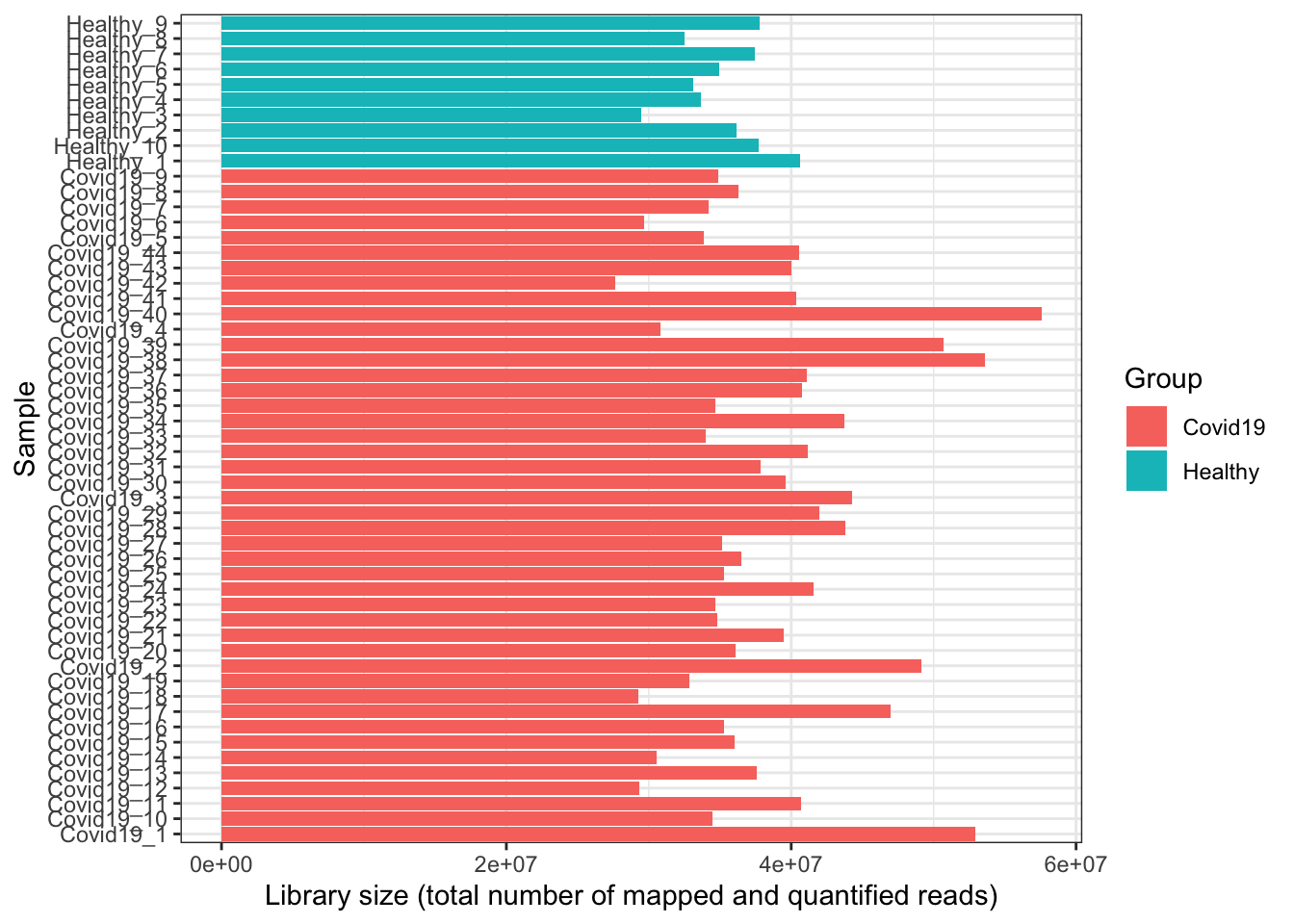
| Version | Author | Date |
|---|---|---|
| f62ae4f | Nhi Hin | 2021-06-30 |
Dimension Reduction
Multi Dimensional Scaling (MDS)
Multi Dimensional Scaling (MDS) is a dimension reduction technique that summarises expression of the top 500 most variable genes expressed in each sample down to 2 dimensions, known as
Dimension 1andDimension 2. Dimension 1 represents the largest amount of variance that can be explained in the data. Plotting these principal components can help us visualise which samples show overall similar gene expression to each other – similar samples will be situated closer to each other on the plot.Because our information is stored in a
DGEListtype of object, we can make use of theglMDSPlotfunction from the Glimma package to make an interactive MDS plot. The MDS plot produced using the function below can be viewed by navigating to theglimma-plotsdirectory and clicking on the MDS-Plot.html file, or by clicking here.
glMDSPlot(dge,
          labels = dge$samples$sample,
          groups = dge$samples$group)
Principal Component Analysis (PCA)
Principal component analysis (PCA) is similar to MDS, but it uses all genes (29302 genes for this particular dataset) to summarise down into a few principal components. Plotting these in the same way as for an MDS plot can also give us information about which samples are similar to each other. In most cases, the MDS and PCA plots will look very similar.
Below, the PCA plot created using the
ggbiplotfunction shows that overall, samples belonging to the samegrouptend to have similar gene expression patterns, and there is quite a large difference betweenHealthyandCovid-19samples. There do not appear to be any obvious outlier samples, although there is quite a bit of variation in gene expression amongstCovid-19samples.We will not remove any samples in this particular dataset as there is no indication so far that any of the samples are obvious outliers.
# Perform PCA analysis:
pca_analysis <- prcomp(t(cpm(dge, log=TRUE)))
summary(pca_analysis)
Importance of components:
PC1 PC2 PC3 PC4 PC5 PC6
Standard deviation 54.2313 33.64178 30.5264 24.6467 22.04485 21.31052
Proportion of Variance 0.2213 0.08514 0.0701 0.0457 0.03656 0.03416
Cumulative Proportion 0.2213 0.30639 0.3765 0.4222 0.45875 0.49292
PC7 PC8 PC9 PC10 PC11 PC12
Standard deviation 18.1218 16.98897 16.60252 15.78163 15.01215 14.43417
Proportion of Variance 0.0247 0.02171 0.02074 0.01874 0.01695 0.01567
Cumulative Proportion 0.5176 0.53933 0.56007 0.57881 0.59576 0.61143
PC13 PC14 PC15 PC16 PC17 PC18
Standard deviation 14.21691 13.67726 13.32318 13.17782 12.95002 12.75765
Proportion of Variance 0.01521 0.01407 0.01335 0.01306 0.01262 0.01224
Cumulative Proportion 0.62664 0.64071 0.65407 0.66713 0.67975 0.69199
PC19 PC20 PC21 PC22 PC23 PC24
Standard deviation 12.58172 12.3644 12.16441 12.14183 12.05517 11.9261
Proportion of Variance 0.01191 0.0115 0.01113 0.01109 0.01093 0.0107
Cumulative Proportion 0.70390 0.7154 0.72653 0.73762 0.74855 0.7592
PC25 PC26 PC27 PC28 PC29 PC30
Standard deviation 11.65802 11.62907 11.57784 11.35174 11.28734 11.22792
Proportion of Variance 0.01022 0.01017 0.01008 0.00969 0.00958 0.00948
Cumulative Proportion 0.76948 0.77965 0.78974 0.79943 0.80901 0.81850
PC31 PC32 PC33 PC34 PC35 PC36
Standard deviation 11.13608 11.0569 10.95973 10.88569 10.71282 10.6322
Proportion of Variance 0.00933 0.0092 0.00904 0.00891 0.00863 0.0085
Cumulative Proportion 0.82783 0.8370 0.84606 0.85498 0.86361 0.8721
PC37 PC38 PC39 PC40 PC41 PC42
Standard deviation 10.58408 10.54698 10.51209 10.33571 10.27164 10.20218
Proportion of Variance 0.00843 0.00837 0.00831 0.00804 0.00794 0.00783
Cumulative Proportion 0.88054 0.88891 0.89722 0.90526 0.91320 0.92103
PC43 PC44 PC45 PC46 PC47 PC48 PC49
Standard deviation 10.15098 10.08666 10.0534 9.90851 9.8527 9.7849 9.6467
Proportion of Variance 0.00775 0.00765 0.0076 0.00739 0.0073 0.0072 0.0070
Cumulative Proportion 0.92878 0.93643 0.9440 0.95142 0.9587 0.9659 0.9729
PC50 PC51 PC52 PC53 PC54
Standard deviation 9.59333 9.52176 9.45986 9.3645 8.843e-14
Proportion of Variance 0.00692 0.00682 0.00673 0.0066 0.000e+00
Cumulative Proportion 0.97985 0.98667 0.99340 1.0000 1.000e+00# Create the plot:
pca_plot <- ggbiplot::ggbiplot(pca_analysis,
groups = dge$samples$group,
ellipse = TRUE,
var.axes = FALSE)
pca_plot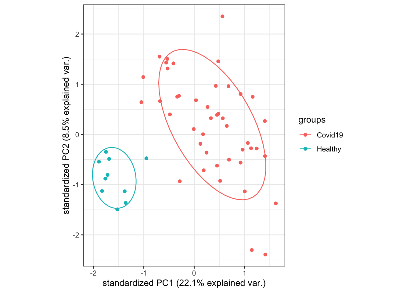
| Version | Author | Date |
|---|---|---|
| f62ae4f | Nhi Hin | 2021-06-30 |
We also have other sample metadata including
ageandsexof the samples in thedge$samplestable. These variables can also be plotted on the PCA plot by changing what is specified in thegroupsargument below, so that we can see whether samples are grouping by age or sex. Doing this is useful as it can tell us whether these variables are confounding variables that have the potential to obscure real biological effects.Below, we can see that the ages of patients from which samples were derived ranges from 51 to 61. It does appear that some of the older patients’ samples are closer to the top of the plot.
ggbiplot::ggbiplot(pca_analysis,
                   groups = dge$samples$age,
                   ellipse = FALSE,
                   var.axes = FALSE)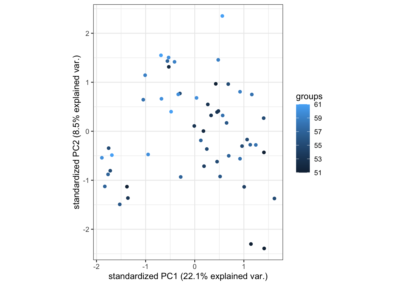
- Below, we can see that
sexof the samples does not seem to really influence where the points lie on the plot, suggesting that sex does not have a noticeable effect on gene expression of the samples here.
ggbiplot::ggbiplot(pca_analysis,
                   groups = dge$samples$sex,
                   ellipse = FALSE,
                   var.axes = FALSE)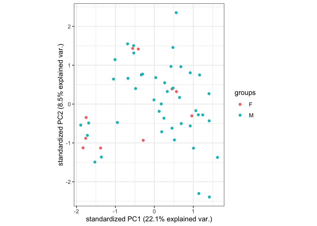
| Version | Author | Date |
|---|---|---|
| 66b2c36 | Nhi Hin | 2021-07-02 |
Questions
- Should we treat male and female samples differently in the analysis, based on the information in the MDS/PCA plots?
- Should we do anything about the older patients’ samples, based on the information in the MDS/PCA plots?
Next Step - Differential gene expression analysis
Overall the data quality looks good and there do not appear to be outlier samples or mislabeled samples.
We will export the DGEList object created in this document for the next step of the analysis, differential gene expression analysis. The
dgeobject is exported into thedata/Rdirectory.
r.dir <- here("data", "R")

ifelse(!dir.exists(r.dir),
       dir.create(r.dir),
       FALSE)

dge %>% saveRDS(file.path(r.dir, "dge.rds"))
sessionInfo()R version 4.0.3 (2020-10-10)
Platform: x86_64-apple-darwin17.0 (64-bit)
Running under: macOS Mojave 10.14.6
Matrix products: default
BLAS: /Library/Frameworks/R.framework/Versions/4.0/Resources/lib/libRblas.dylib
LAPACK: /Library/Frameworks/R.framework/Versions/4.0/Resources/lib/libRlapack.dylib
locale:
[1] en_AU.UTF-8/en_AU.UTF-8/en_AU.UTF-8/C/en_AU.UTF-8/en_AU.UTF-8
attached base packages:
[1] parallel grid stats graphics grDevices utils datasets
[8] methods base
other attached packages:
[1] Glimma_2.0.0 edgeR_3.32.0 limma_3.46.0
[4] AnnotationHub_2.22.0 BiocFileCache_1.14.0 dbplyr_2.1.1
[7] BiocGenerics_0.36.0 export_0.3.0 here_1.0.0
[10] ggrepel_0.8.2 ggbiplot_0.55 scales_1.1.1
[13] plyr_1.8.6 ggplot2_3.3.3 kableExtra_1.3.2
[16] reshape2_1.4.4 tibble_3.1.1 readr_1.4.0
[19] magrittr_2.0.1 dplyr_1.0.5 workflowr_1.6.2
loaded via a namespace (and not attached):
[1] uuid_0.1-4 backports_1.2.0
[3] systemfonts_0.3.2 splines_4.0.3
[5] BiocParallel_1.24.1 crosstalk_1.1.0.1
[7] GenomeInfoDb_1.26.1 digest_0.6.27
[9] htmltools_0.5.1.1 fansi_0.4.1
[11] memoise_1.1.0 openxlsx_4.2.3
[13] annotate_1.68.0 matrixStats_0.57.0
[15] officer_0.3.15 colorspace_2.0-0
[17] blob_1.2.1 rvest_1.0.0
[19] rappdirs_0.3.1 xfun_0.23
[21] crayon_1.4.1 RCurl_1.98-1.2
[23] jsonlite_1.7.2 genefilter_1.72.1
[25] survival_3.2-7 glue_1.4.2
[27] rvg_0.2.5 gtable_0.3.0
[29] zlibbioc_1.36.0 XVector_0.30.0
[31] webshot_0.5.2 DelayedArray_0.16.0
[33] DBI_1.1.0 miniUI_0.1.1.1
[35] Rcpp_1.0.5 viridisLite_0.3.0
[37] xtable_1.8-4 bit_4.0.4
[39] stats4_4.0.3 htmlwidgets_1.5.2
[41] httr_1.4.2 RColorBrewer_1.1-2
[43] ellipsis_0.3.1 farver_2.0.3
[45] pkgconfig_2.0.3 XML_3.99-0.5
[47] sass_0.3.1 locfit_1.5-9.4
[49] utf8_1.1.4 labeling_0.4.2
[51] tidyselect_1.1.0 rlang_0.4.10
[53] manipulateWidget_0.10.1 later_1.1.0.1
[55] AnnotationDbi_1.52.0 munsell_0.5.0
[57] BiocVersion_3.12.0 tools_4.0.3
[59] cli_2.5.0 generics_0.1.0
[61] RSQLite_2.2.1 devEMF_4.0-2
[63] broom_0.7.6 evaluate_0.14
[65] stringr_1.4.0 fastmap_1.0.1
[67] yaml_2.2.1 knitr_1.30
[69] bit64_4.0.5 fs_1.5.0
[71] zip_2.1.1 rgl_0.103.5
[73] purrr_0.3.4 whisker_0.4
[75] mime_0.9 xml2_1.3.2
[77] compiler_4.0.3 rstudioapi_0.13
[79] curl_4.3 interactiveDisplayBase_1.28.0
[81] geneplotter_1.68.0 bslib_0.2.4
[83] stringi_1.5.3 highr_0.8
[85] gdtools_0.2.2 stargazer_5.2.2
[87] lattice_0.20-41 Matrix_1.2-18
[89] vctrs_0.3.7 pillar_1.6.0
[91] lifecycle_1.0.0 BiocManager_1.30.10
[93] jquerylib_0.1.3 data.table_1.13.2
[95] bitops_1.0-6 flextable_0.6.1
[97] httpuv_1.5.4 GenomicRanges_1.42.0
[99] R6_2.5.0 promises_1.1.1
[101] IRanges_2.24.0 assertthat_0.2.1
[103] SummarizedExperiment_1.20.0 DESeq2_1.30.0
[105] rprojroot_2.0.2 withr_2.3.0
[107] S4Vectors_0.28.0 GenomeInfoDbData_1.2.4
[109] hms_1.0.0 tidyr_1.1.3
[111] rmarkdown_2.8 MatrixGenerics_1.2.0
[113] git2r_0.27.1 Biobase_2.50.0
[115] shiny_1.6.0 base64enc_0.1-3