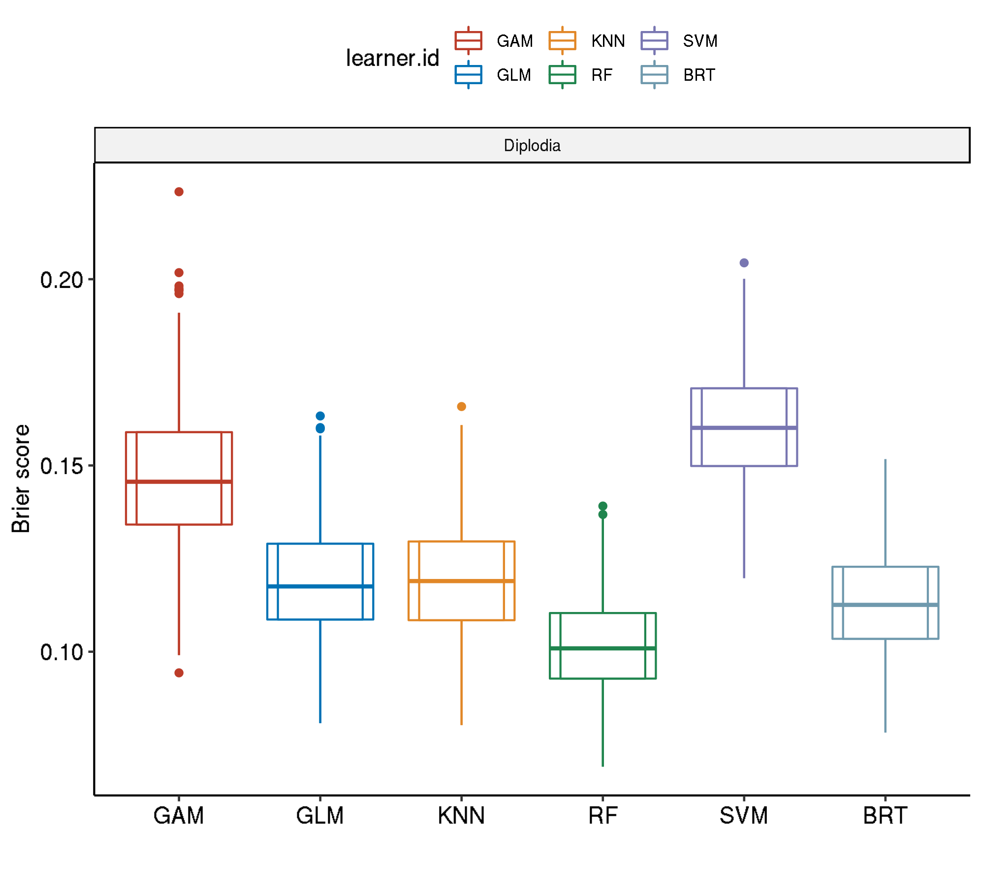
Evaluating classifier performance on Diplodia sapinea
Patrick Schratz, Friedrich-Schiller-University Jena
Last updated: 2019-05-25
Checks: 6 0
Knit directory: 2018-model-comparison/
This reproducible R Markdown analysis was created with workflowr (version 1.3.0). The Checks tab describes the reproducibility checks that were applied when the results were created. The Past versions tab lists the development history.
Great! Since the R Markdown file has been committed to the Git repository, you know the exact version of the code that produced these results.
Great job! The global environment was empty. Objects defined in the global environment can affect the analysis in your R Markdown file in unknown ways. For reproduciblity it’s best to always run the code in an empty environment.
The command set.seed(20190523) was run prior to running the code in the R Markdown file. Setting a seed ensures that any results that rely on randomness, e.g. subsampling or permutations, are reproducible.
Great job! Recording the operating system, R version, and package versions is critical for reproducibility.
Nice! There were no cached chunks for this analysis, so you can be confident that you successfully produced the results during this run.
Great! You are using Git for version control. Tracking code development and connecting the code version to the results is critical for reproducibility. The version displayed above was the version of the Git repository at the time these results were generated.
Note that you need to be careful to ensure that all relevant files for the analysis have been committed to Git prior to generating the results (you can use wflow_publish or wflow_git_commit). workflowr only checks the R Markdown file, but you know if there are other scripts or data files that it depends on. Below is the status of the Git repository when the results were generated:
Ignored files:
    Ignored:    .Rproj.user/
    Ignored:    .drake/
    Ignored:    code/07-paper/._files
    Ignored:    data/
    Ignored:    log/
    Ignored:    packrat/lib-R/
    Ignored:    packrat/lib-ext/
    Ignored:    packrat/lib/
    Ignored:    rosm.cache/
    Ignored:    tests/testthat/

Untracked files:
    Untracked:  analysis/bibliography.bib
    Untracked:  analysis/figure/
    Untracked:  code/07-paper/submission/3/latex-source-files/appendices
    Untracked:  packrat/src/here/

Unstaged changes:
    Modified:   _drake.R
    Modified:   analysis/about.Rmd
    Modified:   analysis/benchmark-pathogens.Rmd
    Modified:   analysis/index.Rmd
    Modified:   analysis/pathogen-maps-debugging.Rmd
    Modified:   analysis/prediction-pathogens.Rmd
    Modified:   code/06-reports.R
    Modified:   code/07-paper/submission/3/latex-source-files/cv_boxplots_final_brier-1.pdf
    Modified:   code/99-packages.R
    Deleted:    docs/figure/benchmark-diplodia.Rmd/cv_boxplots_final_brier-1.pdf
    Modified:   inst/rsync-jupiter.sh
    Modified:   packrat/packrat.lock
Note that any generated files, e.g. HTML, png, CSS, etc., are not included in this status report because it is ok for generated content to have uncommitted changes.
These are the previous versions of the R Markdown and HTML files. If you’ve configured a remote Git repository (see ?wflow_git_remote), click on the hyperlinks in the table below to view them.
| File | Version | Author | Date | Message |
|---|---|---|---|---|
| html | bd443b4 | pat-s | 2019-05-25 | Build site. |
| html | bb74f81 | pat-s | 2019-05-25 | Build site. |
| Rmd | 2fac1aa | pat-s | 2019-05-25 | wflow_publish(knitr_in(“analysis/benchmark-diplodia.Rmd”), view = |
| html | a4a08a2 | pat-s | 2019-05-24 | Build site. |
| Rmd | ac7224e | pat-s | 2019-05-24 | wflow_publish(knitr_in(“analysis/benchmark-diplodia.Rmd”), view = |
| Rmd | 6af4181 | pat-s | 2019-05-23 | update reports |
| Rmd | 769718b | pat-s | 2019-05-23 | Start workflowr project. |
1 Introduction
This document shows the predictive performances for the possible infection risk of trees in the Basque Country by the pathogen Diplodia sapinea.
The following algorithms were benchmarked:
- Boosted Regression Trees (BRT)
- Generalized Additive Model (GAM)
- Generalized Linear Model (GLM)
- k-Nearest Neighbor (KNN)
- Random Forests (RF)
- Support Vector Machine (SVM)
- Extreme Gradient Boosting (XGBOOST)
2 Resampling Strategies
The abbreviations of the tabbed resampling strategies follow the scheme:
<outer resampling> / <inner resampling>
For example, setting “Spatial-Spatial” means that in both levels a “spatial cross-validation” (Brenning (2012)) has been applied.
The inner resampling refers to the hyperparameter tuning level of the nested cross-validation that was applied.
3 Results structure
Teh results are structured as follows:
- Results table of all performances for each resampling setting
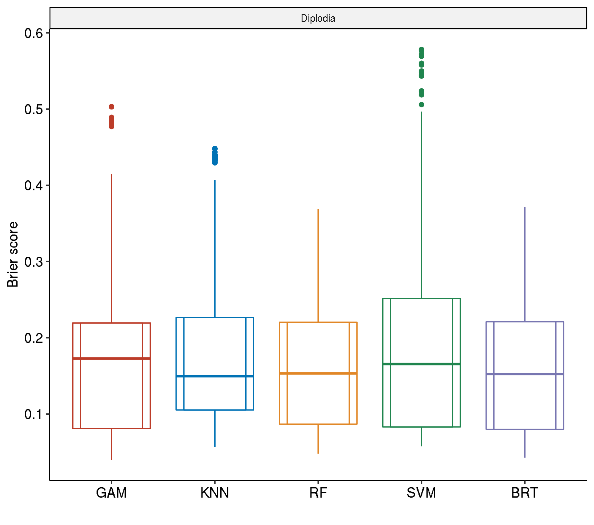
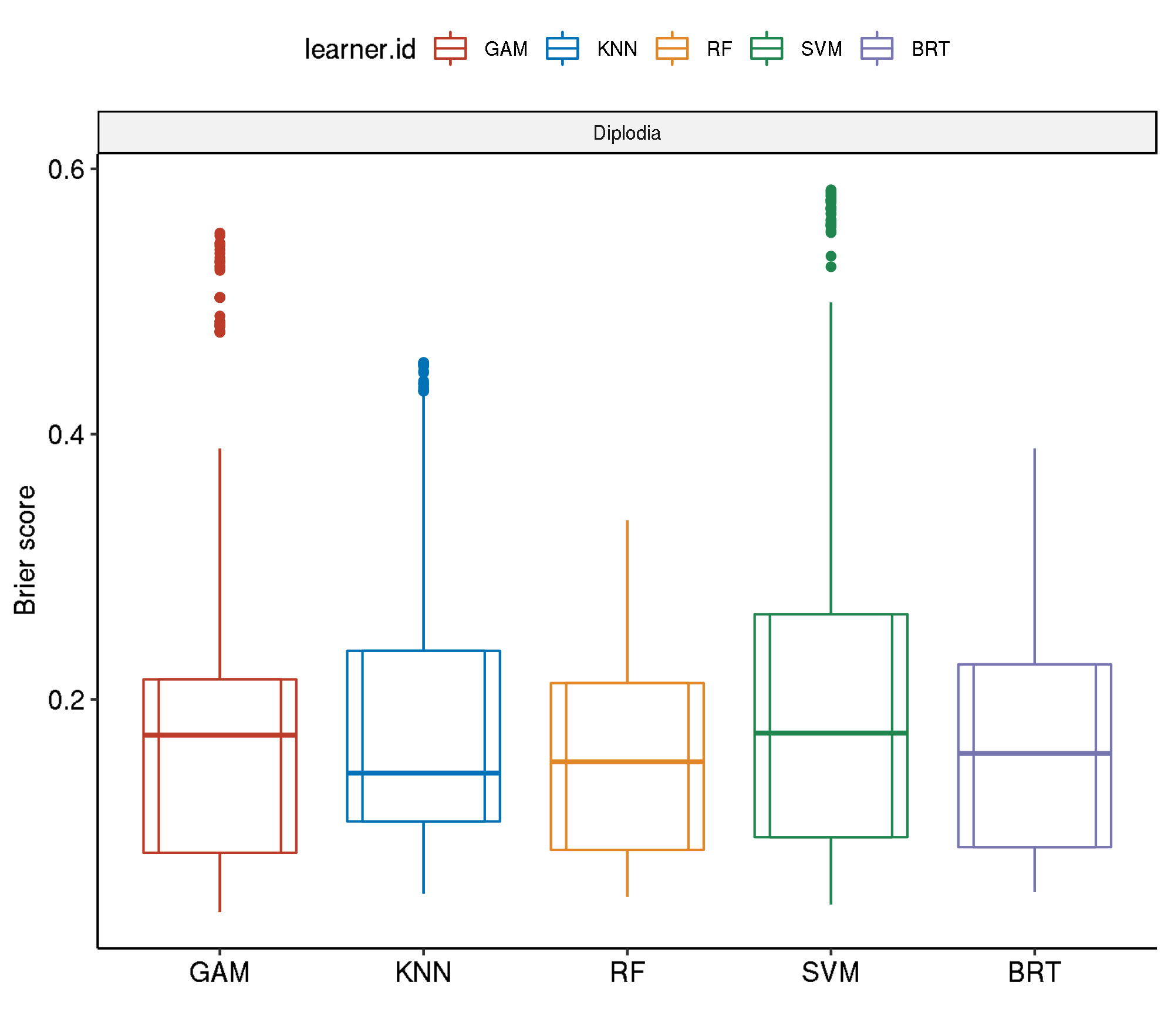
- Boxplot comparison across all algorithms
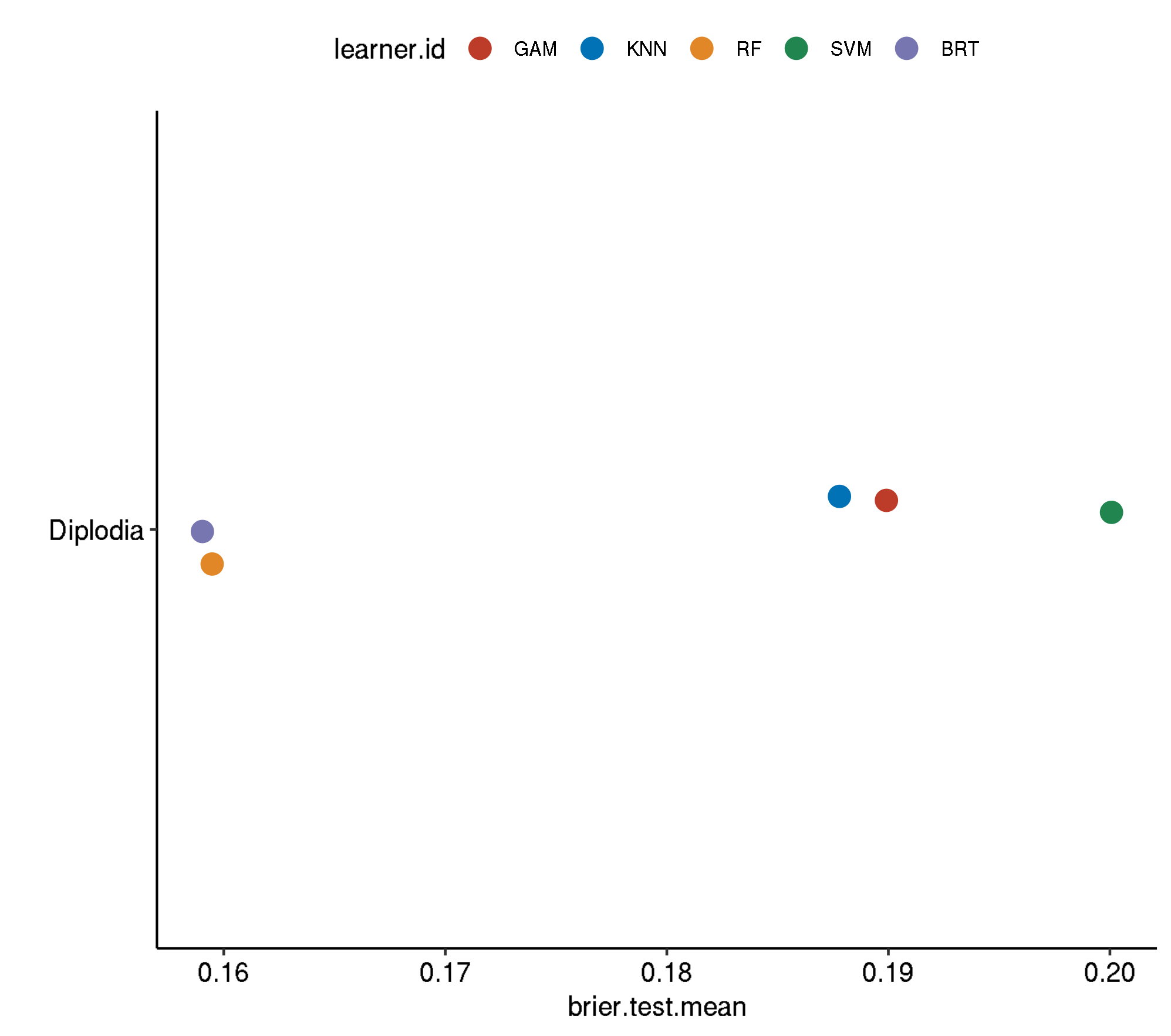
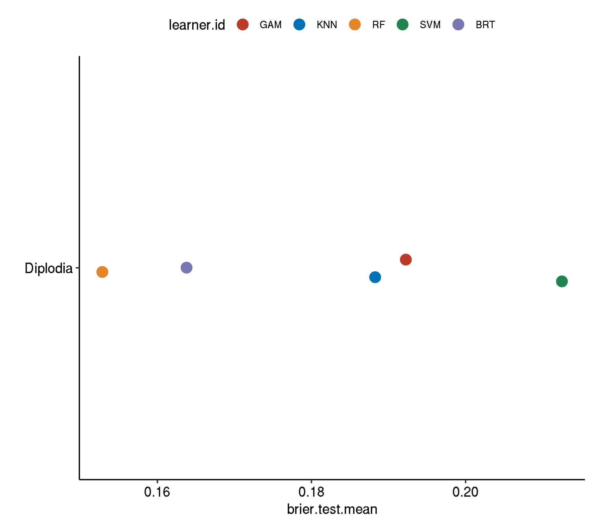
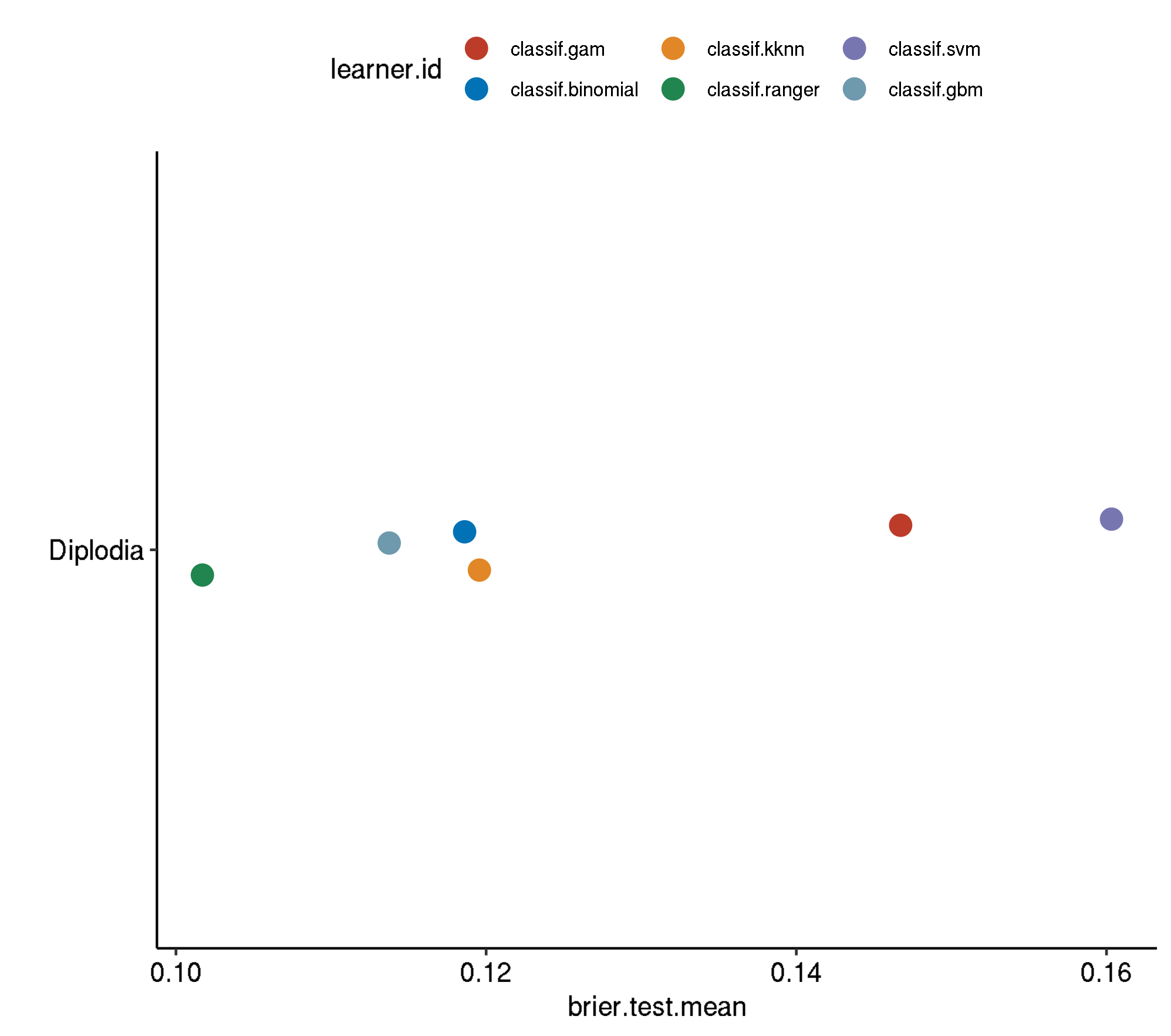
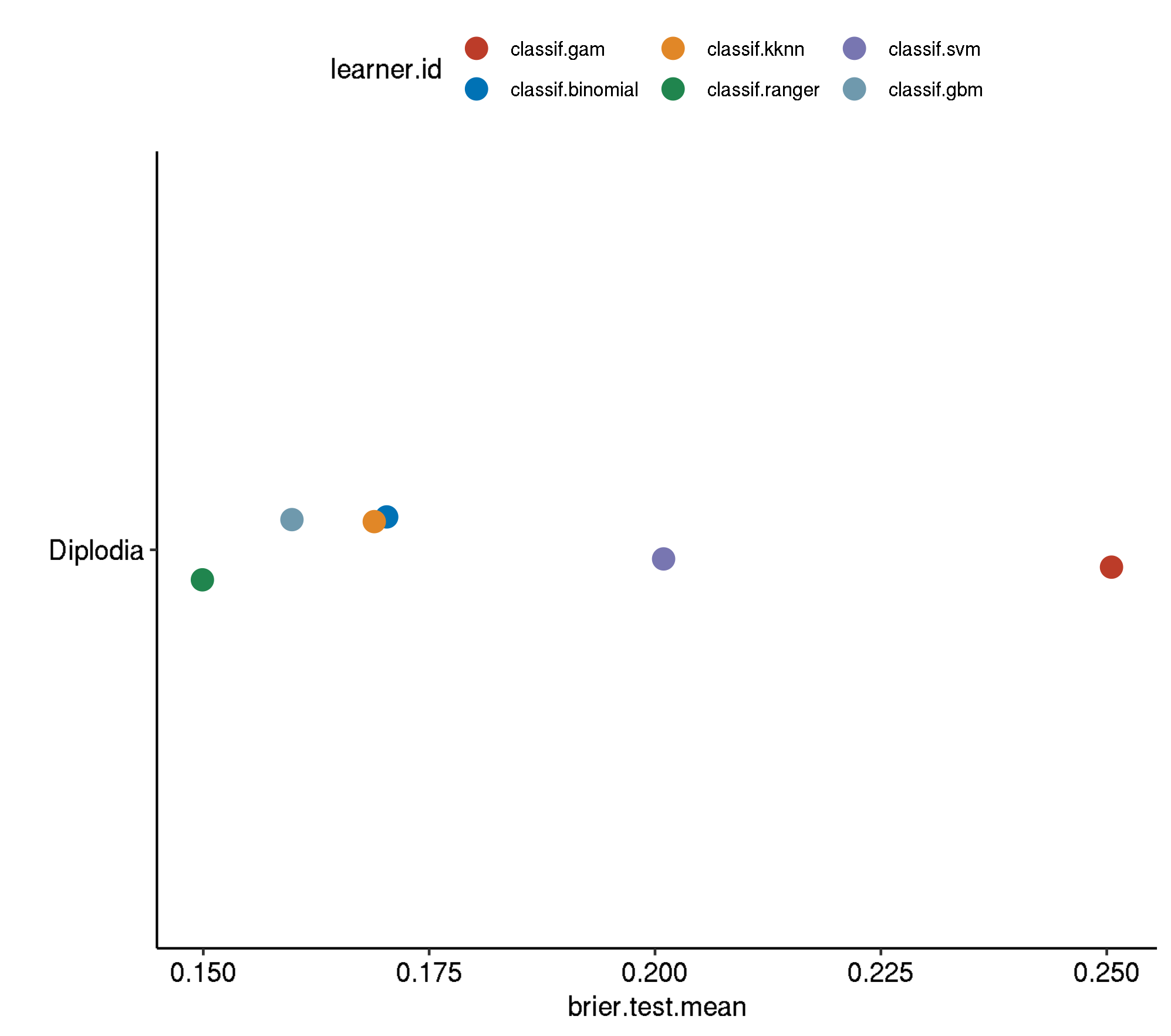
- Aggregated performances across all algorithms
Even though GBM shows the best performance here, RF was the winning model as long as predictor pH was included in the model. This predictor was removed after causing block artifacts in the prediction maps. The following results do not include predictor pH.
# A tibble: 922 x 13
   diplo01  temp precip hail_probability    ph soil  lithology
   <fct>   <dbl>  <dbl>            <dbl> <dbl> <fct> <fct>
 1 0        16.1   249.           0.694   4.06 soil… clastic …
 2 0        16.0   237.           0.646   4.06 soil… clastic …
 3 0        16.0   237.           0.646   4.06 soil… clastic …
 4 0        12.6   152.           0.0238  4.96 soil… chemical…
 5 0        13.8   163.           0.0996  4.96 soil… clastic …
 6 0        13.7   149.           0.0532  5.14 soil… clastic …
 7 0        13.7   146.           0.0637  5.14 soil… clastic …
 8 0        13.8   146.           0.0743  5.14 soil… clastic …
 9 0        13.7   144.           0.0901  5.14 soil… clastic …
10 0        13.9   147.           0.0692  4.98 soil… clastic …
# … with 912 more rows, and 6 more variables: slope_degrees <dbl>,
#   pisr <dbl>, x <dbl>, y <dbl>, year <fct>, age <dbl>
4 Performance results
4.1 Spatial-Spatial
   task.id           learner.id brier.test.mean timetrain.test.mean
1 diplodia    classif.svm.tuned       0.2000721            194.6988
2 diplodia    classif.gam.tuned       0.1899124            230.0244
3 diplodia   classif.kknn.tuned       0.1877918            109.7034
4 diplodia classif.ranger.tuned       0.1594762            240.8807
5 diplodia classif.gbm.tuned 0.1590360 1820.59904.2 Spatial-Non-Spatial
   task.id           learner.id brier.test.mean timetrain.test.mean
1 diplodia    classif.svm.tuned       0.2125015            389.3593
2 diplodia    classif.gam.tuned       0.1922458            294.0095
3 diplodia   classif.kknn.tuned       0.1882630            121.3932
4 diplodia    classif.gbm.tuned       0.1637896           2095.5327
5 diplodia classif.ranger.tuned 0.1528584 445.12064.3 Non-Spatial-Non-Spatial
   task.id           learner.id brier.test.mean timetrain.test.mean
1 diplodia    classif.gam.tuned       0.1395204            290.8944
2 diplodia    classif.svm.tuned       0.1229645            406.3464
3 diplodia   classif.kknn.tuned       0.1201311            121.3484
4 diplodia    classif.gbm.tuned       0.1118638           1999.3005
5 diplodia classif.ranger.tuned 0.0995260 440.40304.4 Non-Spatial-No Tuning
   task.id       learner.id brier.test.mean timetrain.test.mean
1 diplodia      classif.svm       0.1603230            0.638496
2 diplodia      classif.gam       0.1467264            0.615932
3 diplodia     classif.kknn       0.1195669            0.000772
4 diplodia classif.binomial       0.1186126            0.021954
5 diplodia      classif.gbm       0.1137512            0.060954
6 diplodia classif.ranger 0.1017046 0.6675564.5 Spatial-No Tuning
   task.id       learner.id brier.test.mean timetrain.test.mean
1 diplodia      classif.gam       0.2505253            0.569212
2 diplodia      classif.svm       0.2009484            0.627202
3 diplodia classif.binomial       0.1703007            0.022436
4 diplodia     classif.kknn       0.1689237            0.001134
5 diplodia      classif.gbm       0.1598117            0.062854
6 diplodia classif.ranger 0.1499009 0.6519485 Boxplot comparison of all algorithm/tuning settings
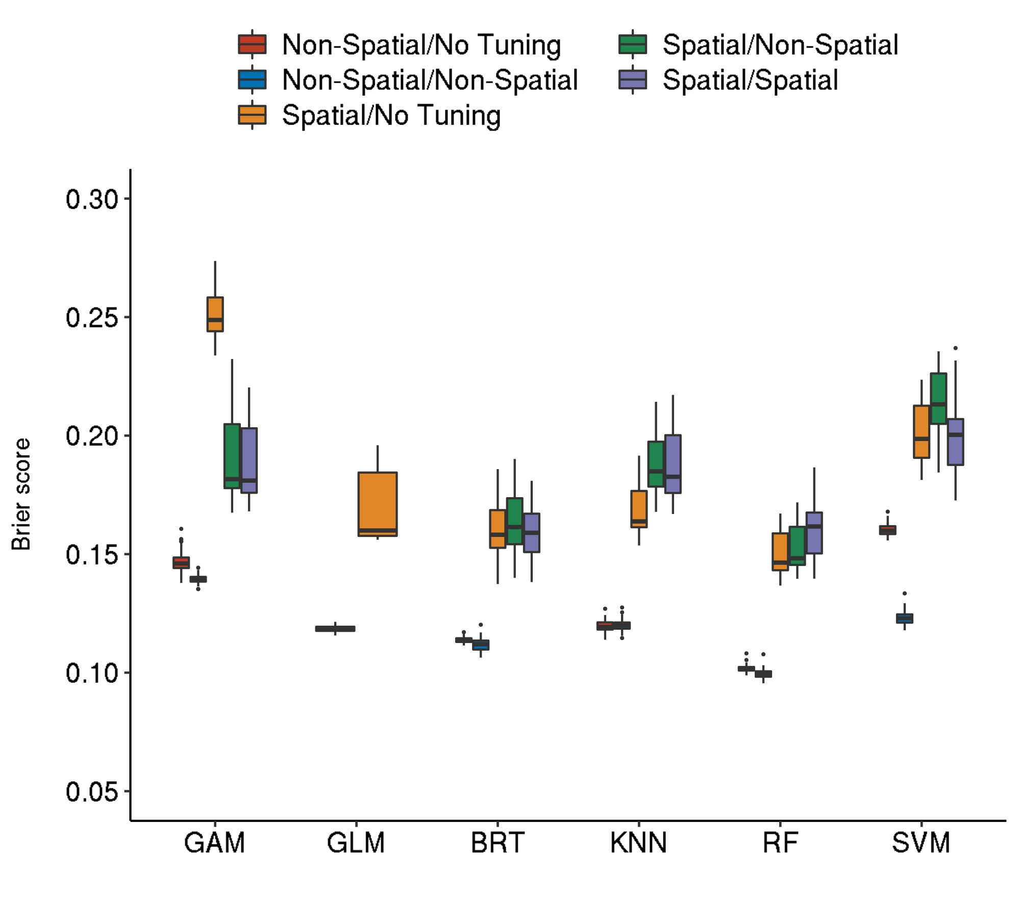
Warning! The custom fig.path you set was ignored by workflowr.
| Version | Author | Date |
|---|---|---|
| a4a08a2 | pat-s | 2019-05-24 |
6 References
Brenning, A. 2012. “Spatial Cross-Validation and Bootstrap for the Assessment of Prediction Rules in Remote Sensing: The R Package Sperrorest.” In 2012 Ieee International Geoscience and Remote Sensing Symposium, 5372–5. https://doi.org/10.1109/IGARSS.2012.6352393.
R version 3.5.1 (2018-07-02)
Platform: x86_64-pc-linux-gnu (64-bit)
Running under: CentOS Linux 7 (Core)

Matrix products: default
BLAS/LAPACK: /opt/spack/opt/spack/linux-centos7-x86_64/gcc-7.3.0/openblas-0.3.5-zncvk4jccaqyfl4z3vszaboeps6hyzta/lib/libopenblas_zen-r0.3.5.so

locale:
 [1] LC_CTYPE=en_GB.UTF-8       LC_NUMERIC=C
 [3] LC_TIME=en_GB.UTF-8        LC_COLLATE=en_GB.UTF-8
 [5] LC_MONETARY=en_GB.UTF-8    LC_MESSAGES=en_GB.UTF-8
 [7] LC_PAPER=en_GB.UTF-8       LC_NAME=C
 [9] LC_ADDRESS=C               LC_TELEPHONE=C
[11] LC_MEASUREMENT=en_GB.UTF-8 LC_IDENTIFICATION=C

attached base packages:
[1] stats     graphics  grDevices utils     datasets  methods   base

other attached packages:
 [1] tidyselect_0.2.5    workflowr_1.3.0     here_0.1
 [4] kableExtra_1.1.0    ggExtra_0.8         ggrepel_0.8.0
 [7] reporttools_1.1.2   xtable_1.8-3        cowplot_0.9.3
[10] hrbrthemes_0.6.0    ggpubr_0.2          future.callr_0.4.0
[13] furrr_0.1.0.9002    future_1.11.1.1     ggsci_2.9
[16] clustermq_0.8.6     ggspatial_1.0.3     ggplot2_3.0.0
[19] rgenoud_5.8-3.0     fs_1.2.6            curl_3.2
[22] R.utils_2.7.0       R.oo_1.22.0         R.methodsS3_1.7.1
[25] GSIF_0.5-5          stringr_1.3.1       RSAGA_1.3.0
[28] plyr_1.8.4          shapefiles_0.7      foreign_0.8-71
[31] gstat_1.1-6         glue_1.3.0          rasterVis_0.45
[34] latticeExtra_0.6-28 RColorBrewer_1.1-2  lattice_0.20-35
[37] raster_2.8-19       viridis_0.5.1       viridisLite_0.3.0
[40] rgdal_1.4-3         sp_1.3-1            tibble_2.0.1
[43] forcats_0.3.0       lwgeom_0.1-6        dplyr_0.8.0.1
[46] sf_0.7-4            parallelMap_1.3     purrr_0.2.5
[49] mlrMBO_1.1.2        smoof_1.5.1         checkmate_1.8.5
[52] BBmisc_1.11         magrittr_1.5        mlr_2.13.9000
[55] ParamHelpers_1.11   drake_7.2.0

loaded via a namespace (and not attached):
  [1] backports_1.1.2   Hmisc_4.2-0       fastmatch_1.1-0
  [4] igraph_1.2.2      lazyeval_0.2.1    splines_3.5.1
  [7] storr_1.2.1       listenv_0.7.0     digest_0.6.15
 [10] htmltools_0.3.6   fansi_0.4.0       base64url_1.4
 [13] cluster_2.0.7-1   readr_1.3.1       globals_0.12.4
 [16] extrafont_0.17    xts_0.11-0        extrafontdb_1.0
 [19] colorspace_1.3-2  rvest_0.3.2       pixmap_0.4-11
 [22] xfun_0.7          callr_3.1.0       crayon_1.3.4
 [25] jsonlite_1.5      hexbin_1.27.2     survival_2.42-3
 [28] zoo_1.8-3         gtable_0.2.0      webshot_0.5.1
 [31] Rttf2pt1_1.3.7    scales_1.0.0      DBI_1.0.0
 [34] miniUI_0.1.1.1    Rcpp_1.0.0        plotrix_3.7-4
 [37] spData_0.2.9.0    htmlTable_1.12    units_0.6-2
 [40] Formula_1.2-3     intervals_0.15.1  dismo_1.1-4
 [43] htmlwidgets_1.3   httr_1.3.1        FNN_1.1
 [46] aqp_1.17          acepack_1.4.1     pkgconfig_2.0.2
 [49] reshape_0.8.8     XML_3.98-1.16     nnet_7.3-12
 [52] utf8_1.1.4        RJSONIO_1.3-1.1   labeling_0.3
 [55] later_0.7.5       rlang_0.3.1       munsell_0.5.0
 [58] tools_3.5.1       cli_1.1.0         evaluate_0.13
 [61] yaml_2.2.0        processx_3.2.1    knitr_1.23
 [64] mime_0.5          whisker_0.3-2     xml2_1.2.0
 [67] compiler_3.5.1    rstudioapi_0.10   plotly_4.8.0
 [70] e1071_1.7-0       spacetime_1.2-2   lhs_0.16
 [73] stringi_1.2.4     ps_1.2.1          gdtools_0.1.7
 [76] plot3D_1.1.1      Matrix_1.2-14     classInt_0.2-3
 [79] pillar_1.3.1      plotKML_0.5-9     data.table_1.11.8
 [82] httpuv_1.4.5      colorRamps_2.3    R6_2.2.2
 [85] promises_1.0.1    gridExtra_2.3     codetools_0.2-15
 [88] MASS_7.3-50       assertthat_0.2.0  rprojroot_1.3-2
 [91] withr_2.1.2       hms_0.4.2         parallel_3.5.1
 [94] grid_3.5.1        rpart_4.1-13      tidyr_0.8.2
 [97] class_7.3-14      rmarkdown_1.12    misc3d_0.8-4
[100] mco_1.0-15.1      git2r_0.23.0      shiny_1.2.0
[103] base64enc_0.1-3 