Node summary
Robert Schlegel
2019-07-09
Last updated: 2019-08-07
workflowr checks: (Click a bullet for more information)-
✔ R Markdown file: up-to-date
Great! Since the R Markdown file has been committed to the Git repository, you know the exact version of the code that produced these results.
-
✔ Environment: empty
Great job! The global environment was empty. Objects defined in the global environment can affect the analysis in your R Markdown file in unknown ways. For reproduciblity it’s best to always run the code in an empty environment.
-
✔ Seed:
set.seed(20190513)The command
set.seed(20190513)was run prior to running the code in the R Markdown file. Setting a seed ensures that any results that rely on randomness, e.g. subsampling or permutations, are reproducible. -
✔ Session information: recorded
Great job! Recording the operating system, R version, and package versions is critical for reproducibility.
-
Great! You are using Git for version control. Tracking code development and connecting the code version to the results is critical for reproducibility. The version displayed above was the version of the Git repository at the time these results were generated.✔ Repository version: 9d81722
Note that you need to be careful to ensure that all relevant files for the analysis have been committed to Git prior to generating the results (you can usewflow_publishorwflow_git_commit). workflowr only checks the R Markdown file, but you know if there are other scripts or data files that it depends on. Below is the status of the Git repository when the results were generated:
Note that any generated files, e.g. HTML, png, CSS, etc., are not included in this status report because it is ok for generated content to have uncommitted changes.Ignored files: Ignored: .Rhistory Ignored: .Rproj.user/ Ignored: data/ALL_anom.Rda Ignored: data/ALL_clim.Rda Ignored: data/ERA5_lhf.Rda Ignored: data/ERA5_lwr.Rda Ignored: data/ERA5_qnet.Rda Ignored: data/ERA5_qnet_anom.Rda Ignored: data/ERA5_qnet_clim.Rda Ignored: data/ERA5_shf.Rda Ignored: data/ERA5_swr.Rda Ignored: data/ERA5_t2m.Rda Ignored: data/ERA5_t2m_anom.Rda Ignored: data/ERA5_t2m_clim.Rda Ignored: data/ERA5_u.Rda Ignored: data/ERA5_u_anom.Rda Ignored: data/ERA5_u_clim.Rda Ignored: data/ERA5_v.Rda Ignored: data/ERA5_v_anom.Rda Ignored: data/ERA5_v_clim.Rda Ignored: data/GLORYS_mld.Rda Ignored: data/GLORYS_mld_anom.Rda Ignored: data/GLORYS_mld_clim.Rda Ignored: data/GLORYS_u.Rda Ignored: data/GLORYS_u_anom.Rda Ignored: data/GLORYS_u_clim.Rda Ignored: data/GLORYS_v.Rda Ignored: data/GLORYS_v_anom.Rda Ignored: data/GLORYS_v_clim.Rda Ignored: data/NAPA_clim_U.Rda Ignored: data/NAPA_clim_V.Rda Ignored: data/NAPA_clim_W.Rda Ignored: data/NAPA_clim_emp_ice.Rda Ignored: data/NAPA_clim_emp_oce.Rda Ignored: data/NAPA_clim_fmmflx.Rda Ignored: data/NAPA_clim_mldkz5.Rda Ignored: data/NAPA_clim_mldr10_1.Rda Ignored: data/NAPA_clim_qemp_oce.Rda Ignored: data/NAPA_clim_qla_oce.Rda Ignored: data/NAPA_clim_qns.Rda Ignored: data/NAPA_clim_qsb_oce.Rda Ignored: data/NAPA_clim_qt.Rda Ignored: data/NAPA_clim_runoffs.Rda Ignored: data/NAPA_clim_ssh.Rda Ignored: data/NAPA_clim_sss.Rda Ignored: data/NAPA_clim_sst.Rda Ignored: data/NAPA_clim_taum.Rda Ignored: data/NAPA_clim_vars.Rda Ignored: data/NAPA_clim_vecs.Rda Ignored: data/OAFlux.Rda Ignored: data/OISST_sst.Rda Ignored: data/OISST_sst_anom.Rda Ignored: data/OISST_sst_clim.Rda Ignored: data/node_mean_all_anom.Rda Ignored: data/packet_all.Rda Ignored: data/packet_all_anom.Rda Ignored: data/packet_nolab.Rda Ignored: data/packet_nolab14.Rda Ignored: data/packet_nolabgsl.Rda Ignored: data/packet_nolabmod.Rda Ignored: data/som_all.Rda Ignored: data/som_all_anom.Rda Ignored: data/som_nolab.Rda Ignored: data/som_nolab14.Rda Ignored: data/som_nolab_16.Rda Ignored: data/som_nolab_9.Rda Ignored: data/som_nolabgsl.Rda Ignored: data/som_nolabmod.Rda Ignored: data/synoptic_states.Rda Ignored: data/synoptic_vec_states.Rda Unstaged changes: Modified: code/workflow.R
Expand here to see past versions:
| File | Version | Author | Date | Message |
|---|---|---|---|---|
| Rmd | 9d81722 | robwschlegel | 2019-08-07 | Re-publish entire site. |
| Rmd | ed626bf | robwschlegel | 2019-08-07 | Ran a bunch of figures and had a meeting with Eric. More changes coming to GLORYS data tomorrow before settling on one of the experimental SOMs |
| html | d4ba012 | robwschlegel | 2019-07-09 | Build site. |
| Rmd | c8a5a1a | robwschlegel | 2019-07-09 | Fixing figure display in vignette. |
| Rmd | 3a740c2 | robwschlegel | 2019-07-09 | Creating assets folder for displaying figures created in other vignettes in new vignettes etc. |
| html | 3a740c2 | robwschlegel | 2019-07-09 | Creating assets folder for displaying figures created in other vignettes in new vignettes etc. |
| html | 81e961d | robwschlegel | 2019-07-09 | Build site. |
| Rmd | 497eeb2 | robwschlegel | 2019-07-09 | Re-publish entire site. |
| Rmd | 95a168d | robwschlegel | 2019-07-09 | Frame of node summary vignette worked out |
Introduction
This vignette will show the summary figures for the various SOM experiments. The code used to create these summary figures may be found in code/functions.R and a more detailed overview is given in the Figures vignette. The nodes are listed below by their number. Use the table of contents on the left of the screen to move qucikly between nodes of interest as desired.
Visualise SOM results
With the following lines of code we create PDFs for each of the variables for each of the nodes for our different conditions. These PDFs may be seen at output/SOM/*, where * is the code name denoting which SOM experiment was conducted.
Juggling back and forth between the SST anomaly photos with and without the Gulf of St Lawrence it first appears that they are very different, but this is mostly due to the top and bottom rows of nodes being flipped. The actual differences are much more muted and the patterns tend to hold. The patterns appear more crisp in the larger of the two study extents. This is likely because the inclusion of the shallow GSL gives more power to the atmospheric variables to compete with the Gulf Stream. For this reason we are going to proceed with the inclusion of the Gulf of St Lawrence.
Looking at different counts of nodes it appears as though 9 is not enough. When 12 nodes are used more detail comes through. Going up to 16 nodes appear to be too much as not much more detail comes through while creating the complexity of more node results to sift through. When the moderate events are removed we are left with only 37 events (synoptic states) to feed the SOM. This means we shouldn’t use more than 4 nodes so as not to (be just shy of) at least 10 potential values binned into each node. The four nodes that are output do show the most clear difference in patterns and actually do a surprising job of ecapsulating the different potential drivers of MHWs. An ANOSIM test on the nodes show that they are different with a p = 0.046. All of the other results have a ANOSIM of p = 0.001. One issue with screening the events by category is that this part of the ocean experiences many long category I Moderate events that may still be relevant.
So rather than screen by category, I also made a run on the SOM with MHW data with events shorter than 14 days removed. This left us with 103 events to work with, whcih is a good number to use with a 3x3 grid. The results tell perhaps a clearer story than with the 12 nodes and all MHWs.
Just from looking at the node summaries created in this vignette it is too difficult to say conclusively which conditional produces the clearest results. We will need to proceed with the creation of the more in depth node summary figures in order to get a better idea of how well this is working out. Also unresolved in this vignette is the criticism that the methodology used for the creation of the mean synoptic states fed to the SOM is weak to long events coming through as “grey”, meaning they average out to a rather unremarkable state, even though they are likely the most important of all. One proposed fix for this is to create synoptic states using only the peak date of the event, rather than a mean over the range of the event. This should be looked into…
A last point here is also that this methodology should also be useful for looking backwards and forwards through time to see what the synoptic states looked like leading up to and just after the event. This information could be more useful than the first wave of results. Before doing this however a singular methodology needs to be pinned down (i.e. which events to screen and how many nodes to use).
See the files in the /output/SOM_nodes/ folder in the GitHub repo for this project. They aren’t all shown here because they take a bit too long to render.
Node summary table
The table below contains a concise summary of the nodes from the more promising SOM experiments.
| Node | Region | Season | MHW Properties | Conditions |
|---|---|---|---|---|
| 1 | LS | Australia | Spicey | All of the things |
Figure caption key
The captions for the figures below have a lot of acronyms in them but they are consistently used and I will provide a list of what they are here. Whenever one sees an acronym in lower case letters it is refering to one of the regions of the study area as seen in the following figure.
The region abbreviations are:
- gm = Gulf of Maine
- gls = Gulf of St. Lawrence
- ls = Labrador Shelf
- mab = Mid-Atlantic Bight
- nfs = Newfoundland Shelf
- ss = Scotian Shelf
The upper case acronyms used in the following figure captions are as follows:
- SST = Sea surface temperature
- SOM = Self-organising map(s)
- GS = Gulf Stream
- AO = Atlantic Ocean
- LS = Labrador Sea
- LC = Labrador Current
- NS = Nova Scotia
If I have missed any please don’t hesitate to send me a message.
SST overview
The figure below shows the SST anomaly per node as a means of providing a very general overview of what each node looks like so as to make navigating between them more convenient.
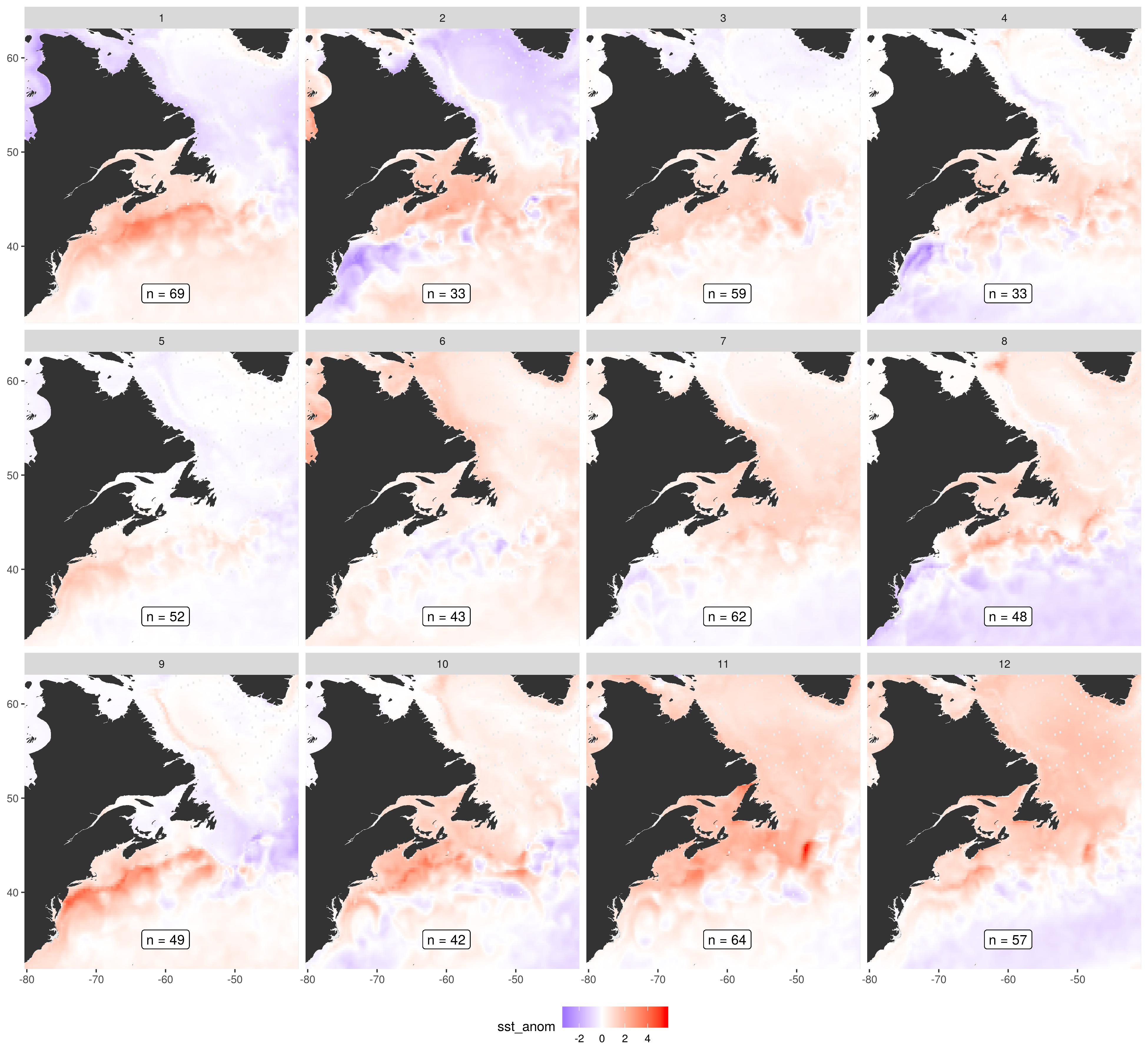
The SST anomaly per node of the SOM. Note that the SST patterns are calculated in conjunction with the several other variables and are not the only variable taken into account. They are shown here by themselves as I think they provide the most convenient single snap shot of the results.
Expand here to see past versions of som_plot_sst_anom.png:
| Version | Author | Date |
|---|---|---|
| 69e8001 | robwschlegel | 2019-07-09 |
Node 1
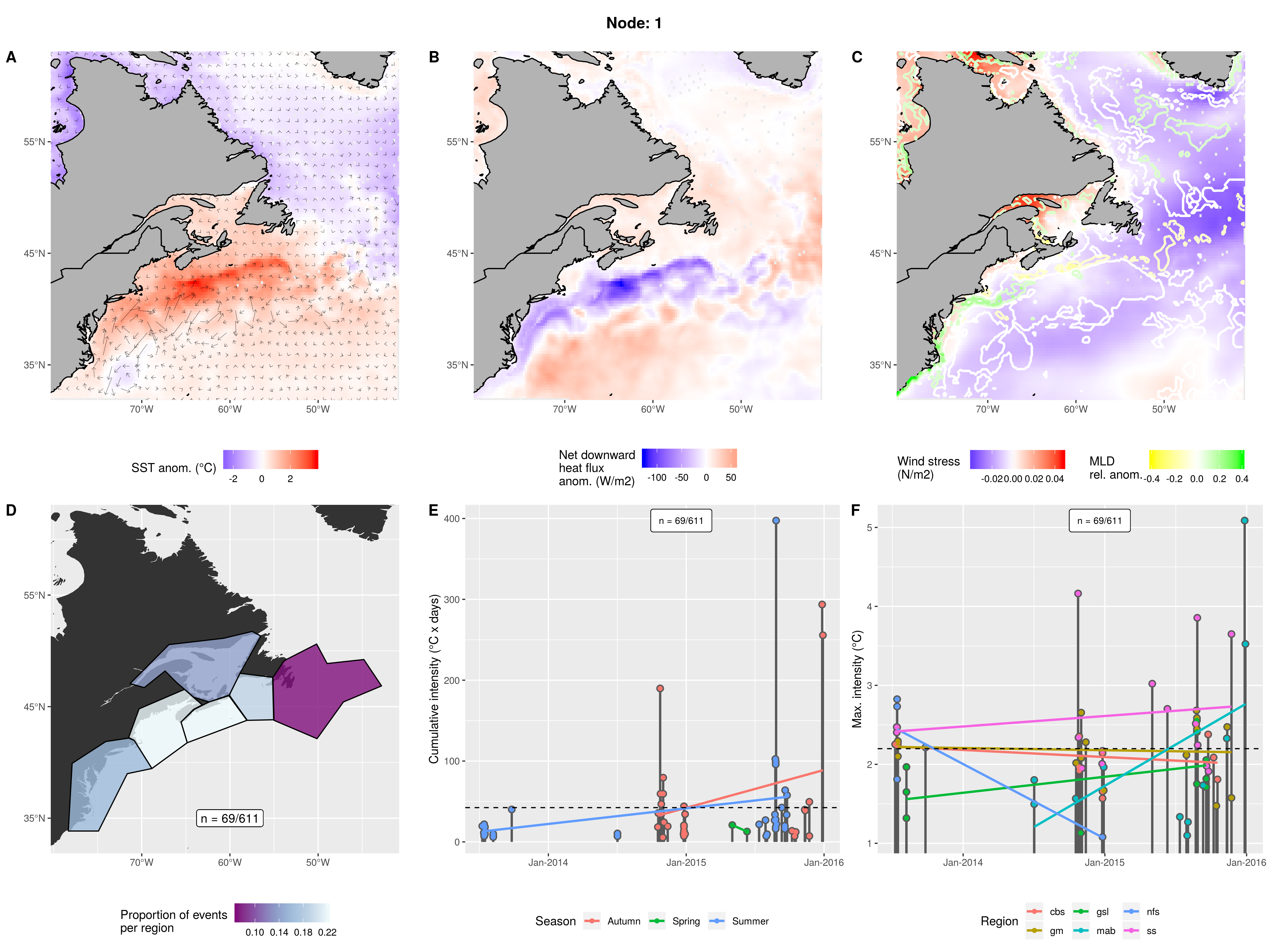
Warm pulse of GS near the NS coast. Shallowing mixed layer, low wind stress, and strong negative heat flux. Mostly gm and ss, almost no nfs. Almost entirely summer and autumn from 2013 - 2016. Mostly smaller evets but a few are massive.
Expand here to see past versions of node_1_panels.png:
| Version | Author | Date |
|---|---|---|
| 69e8001 | robwschlegel | 2019-07-09 |
Node 2
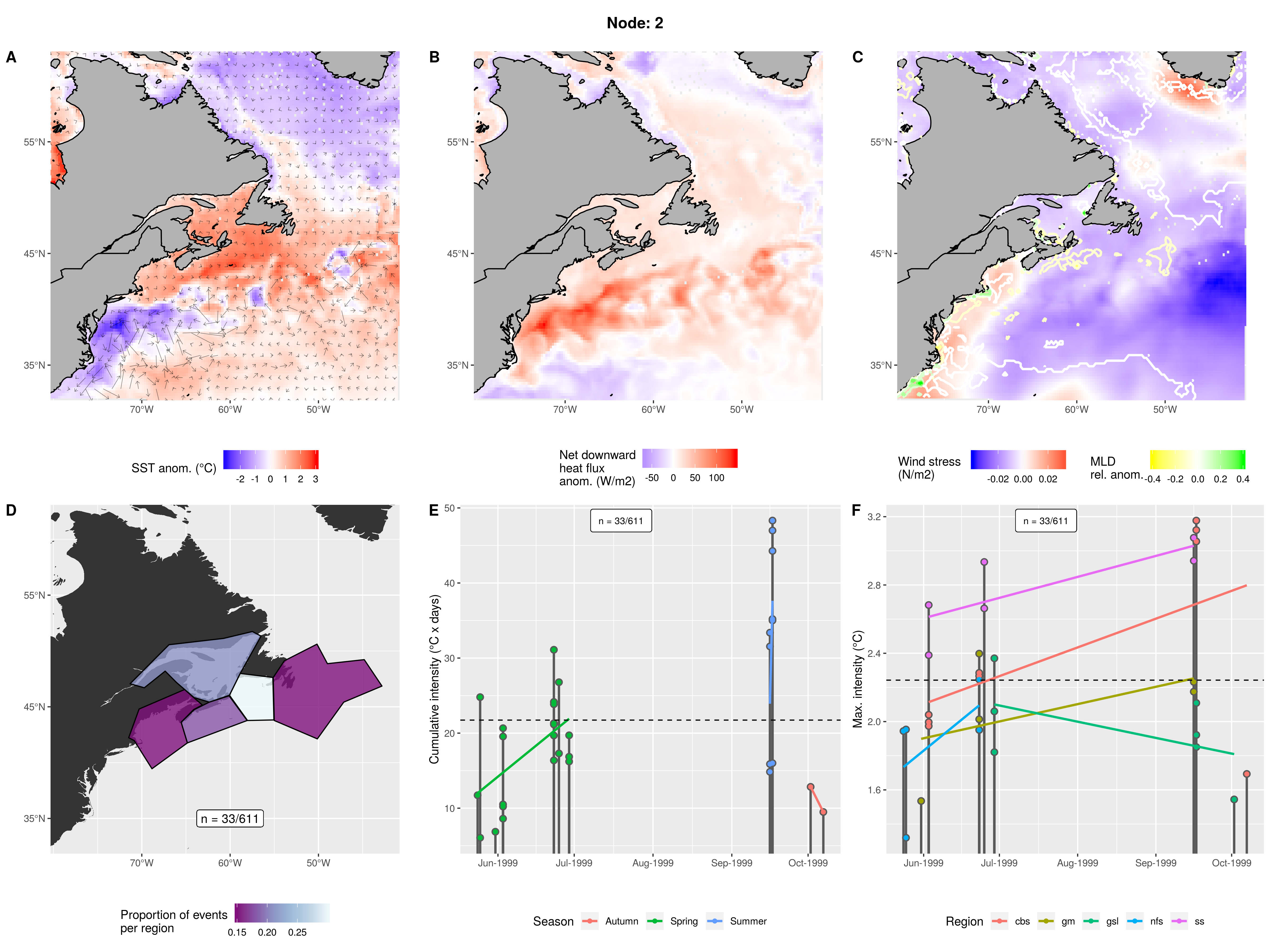
Cold GS with warm LC caused by positive heat flux, low wind stress, and shallow mixed layer. Mostly cbs with some gsl and no mab. Occurred in only one year in two pulses in spring and summer. Normal intensity but short duration.
Expand here to see past versions of node_2_panels.png:
| Version | Author | Date |
|---|---|---|
| 69e8001 | robwschlegel | 2019-07-09 |
Node 3
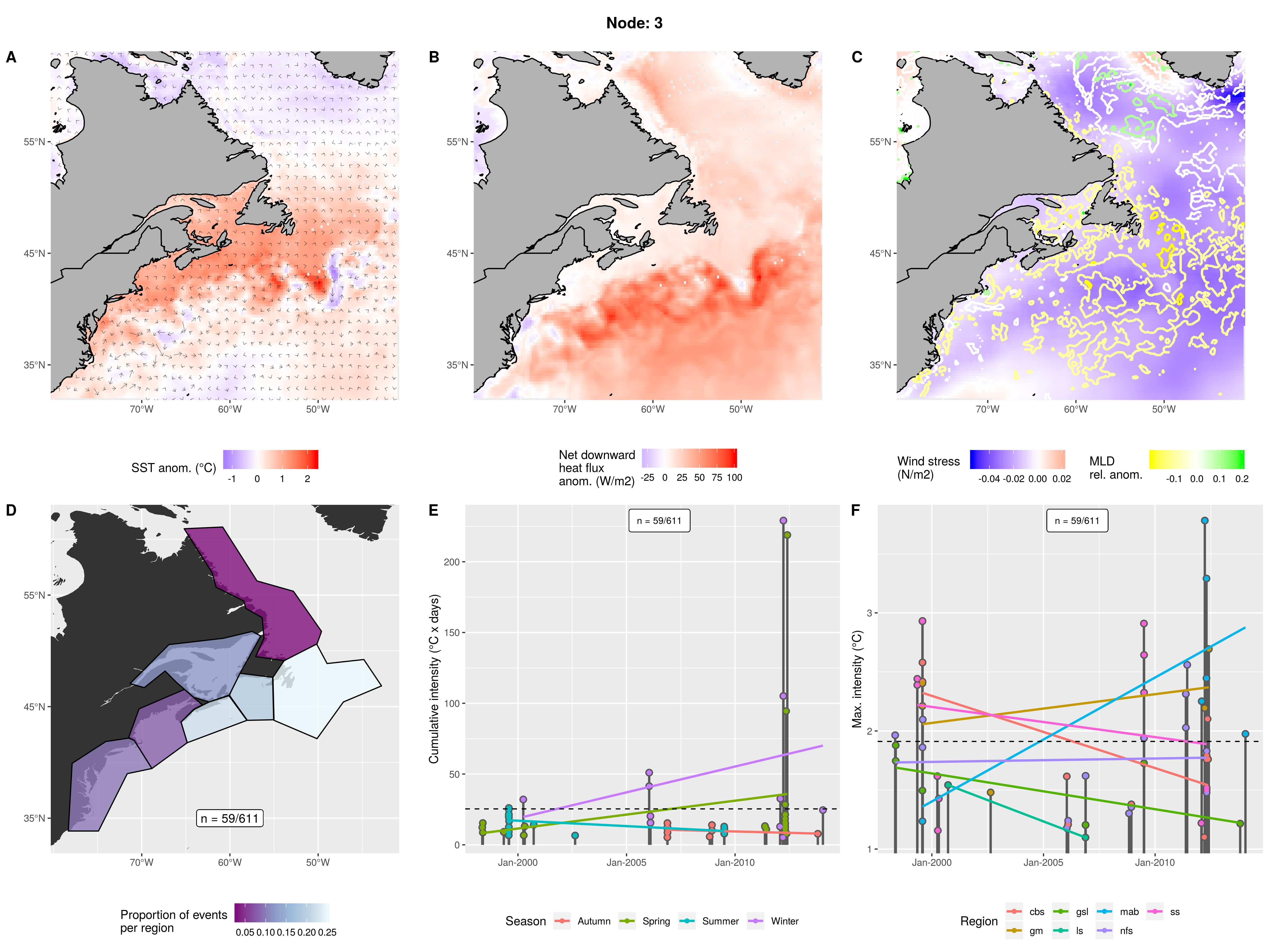
Calm sea state with some positive heatflux into the LC causing events. Shallower mixed layer everywhere. Mostly nfs with progressively fewer events in regions down the coast. Almost none in ls. Smaller events with a couple of large ones. All seasons from 1999 - 2014.
Expand here to see past versions of node_3_panels.png:
| Version | Author | Date |
|---|---|---|
| 69e8001 | robwschlegel | 2019-07-09 |
Node 4
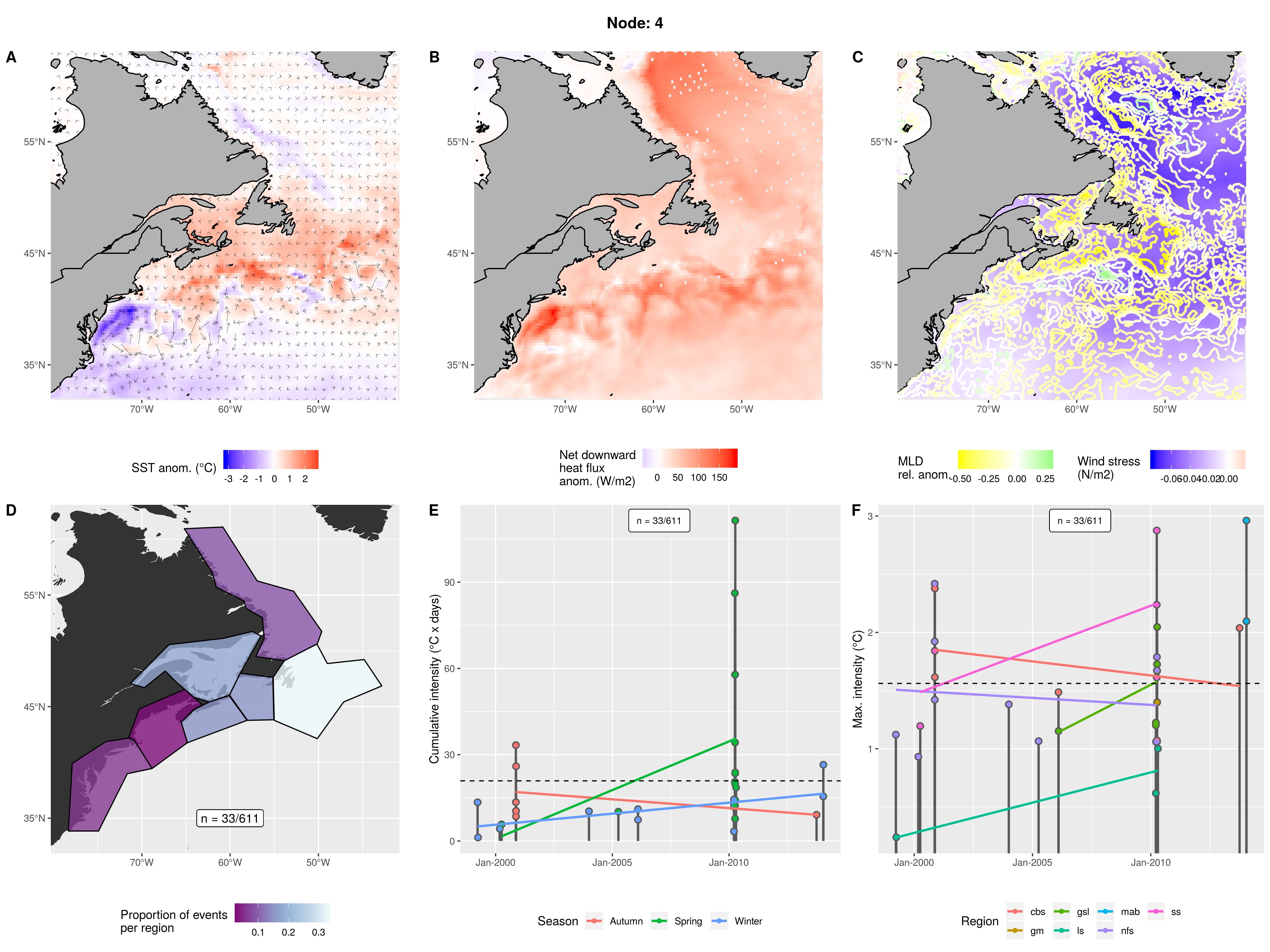
Extremely shallow mixed layer with a strong positive heatflux and low wind stress. Mostly nfs with progressively fewer events further away. Smaller events. Autumn, Winter, and Spring from 1999 - 2014.
Expand here to see past versions of node_4_panels.png:
| Version | Author | Date |
|---|---|---|
| 69e8001 | robwschlegel | 2019-07-09 |
Node 5
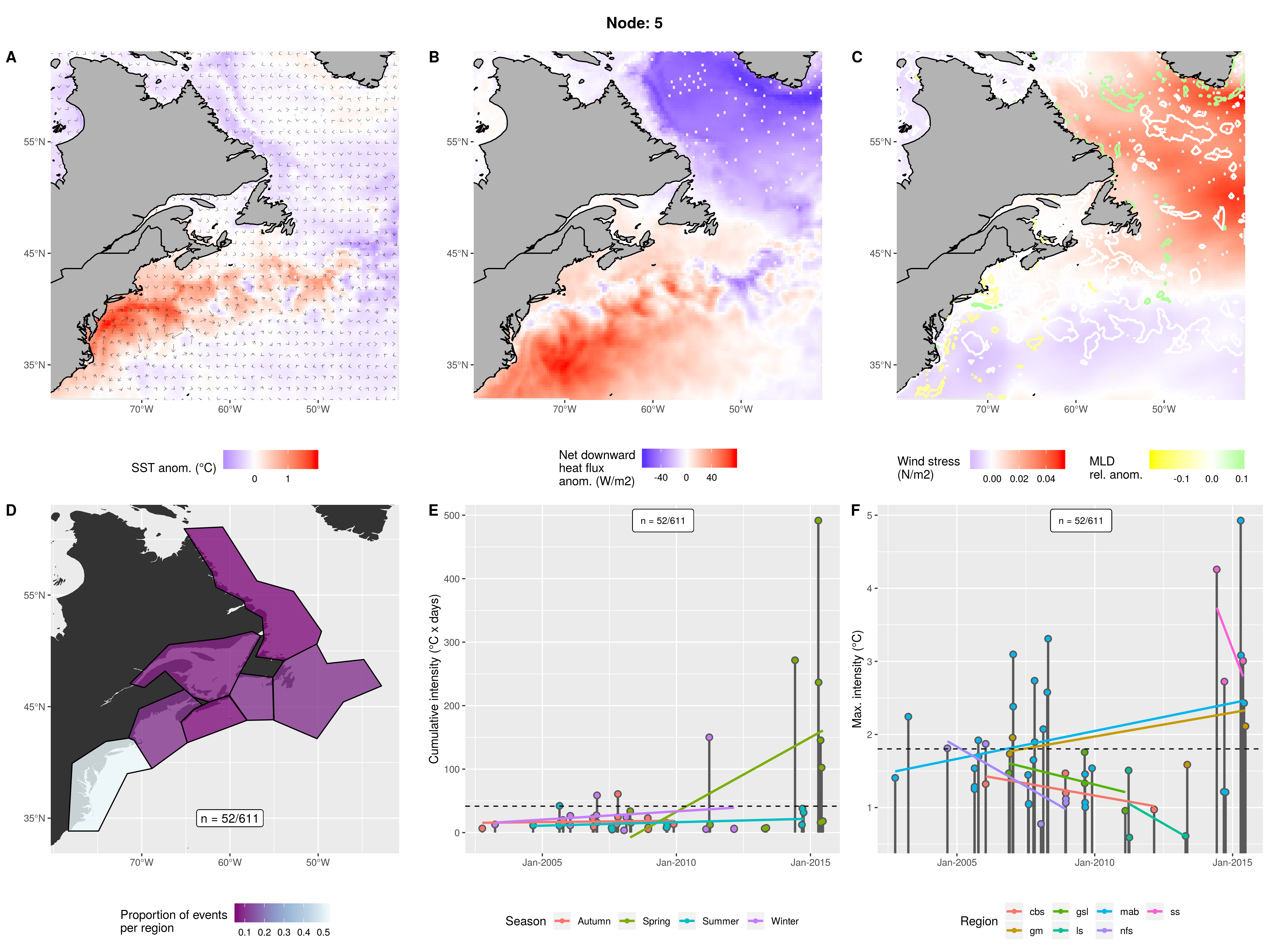
Slightly shallow slightly fast push of the GS into the coast becoming slightly deeper near WHOI before coming back away from the coast and chilling out. The core of the pulse has negative heatflux but the surrounding GS has a strong positive heatflux and snall wind stress. Almost exclusively occurs in mab with only a bit everywhere else. Smallish events with a few massive ones. All seasons from 2003 - 2015.
Expand here to see past versions of node_5_panels.png:
| Version | Author | Date |
|---|---|---|
| 69e8001 | robwschlegel | 2019-07-09 |
Node 6
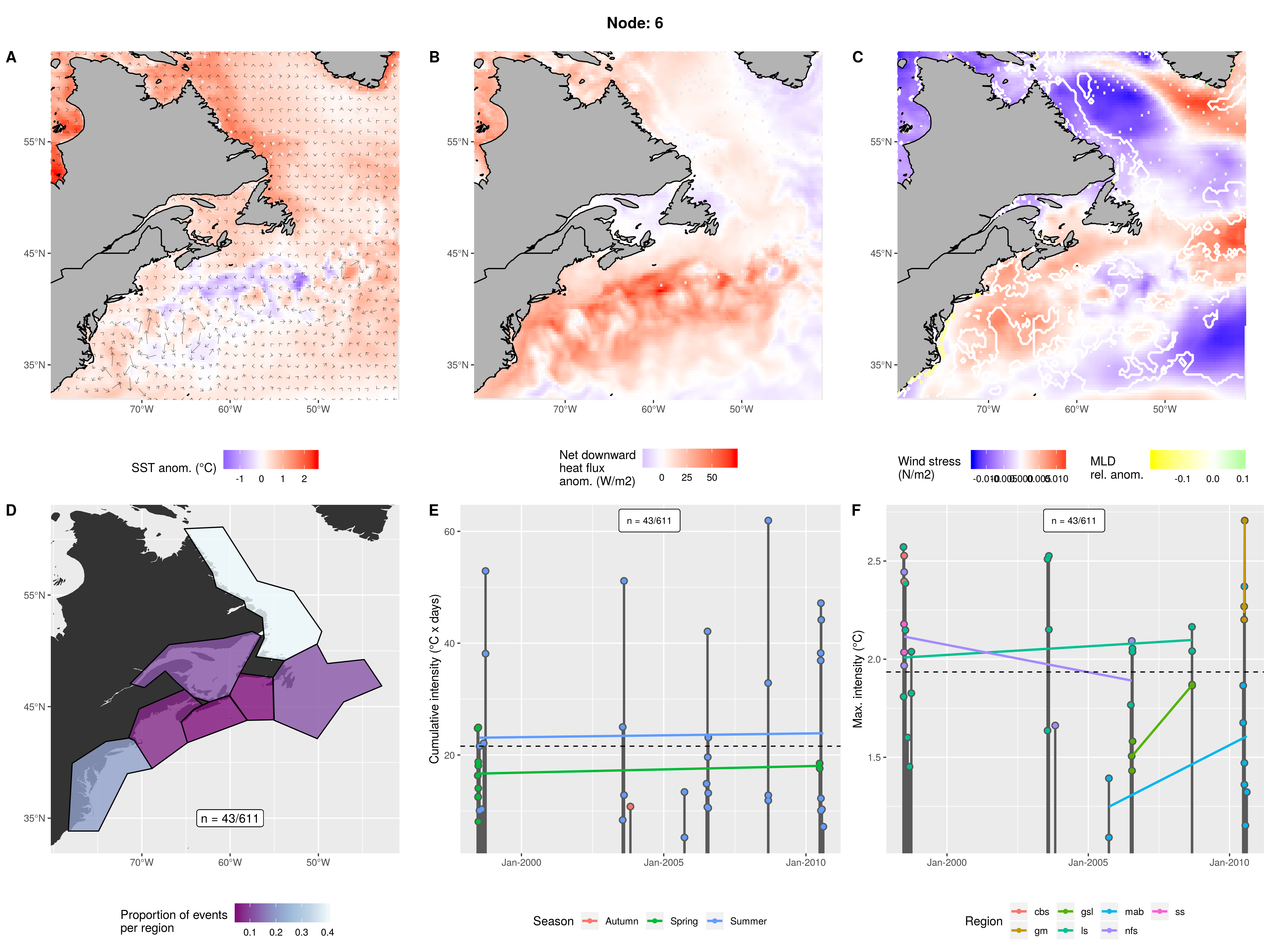
Slightly warmer LS and LC with cooler GS. Minor poitive heat flux into LS and large positive heat flux into GS. Normal mixed layer with low wind stress over the LS and high over the GS. Mostly in the ls with a bit in the mab with almost none elsewhere. Occurred over 1999 - 2010 in spring and summer. Smaller events that have not been increasing over time.
Expand here to see past versions of node_6_panels.png:
| Version | Author | Date |
|---|---|---|
| 69e8001 | robwschlegel | 2019-07-09 |
Node 7
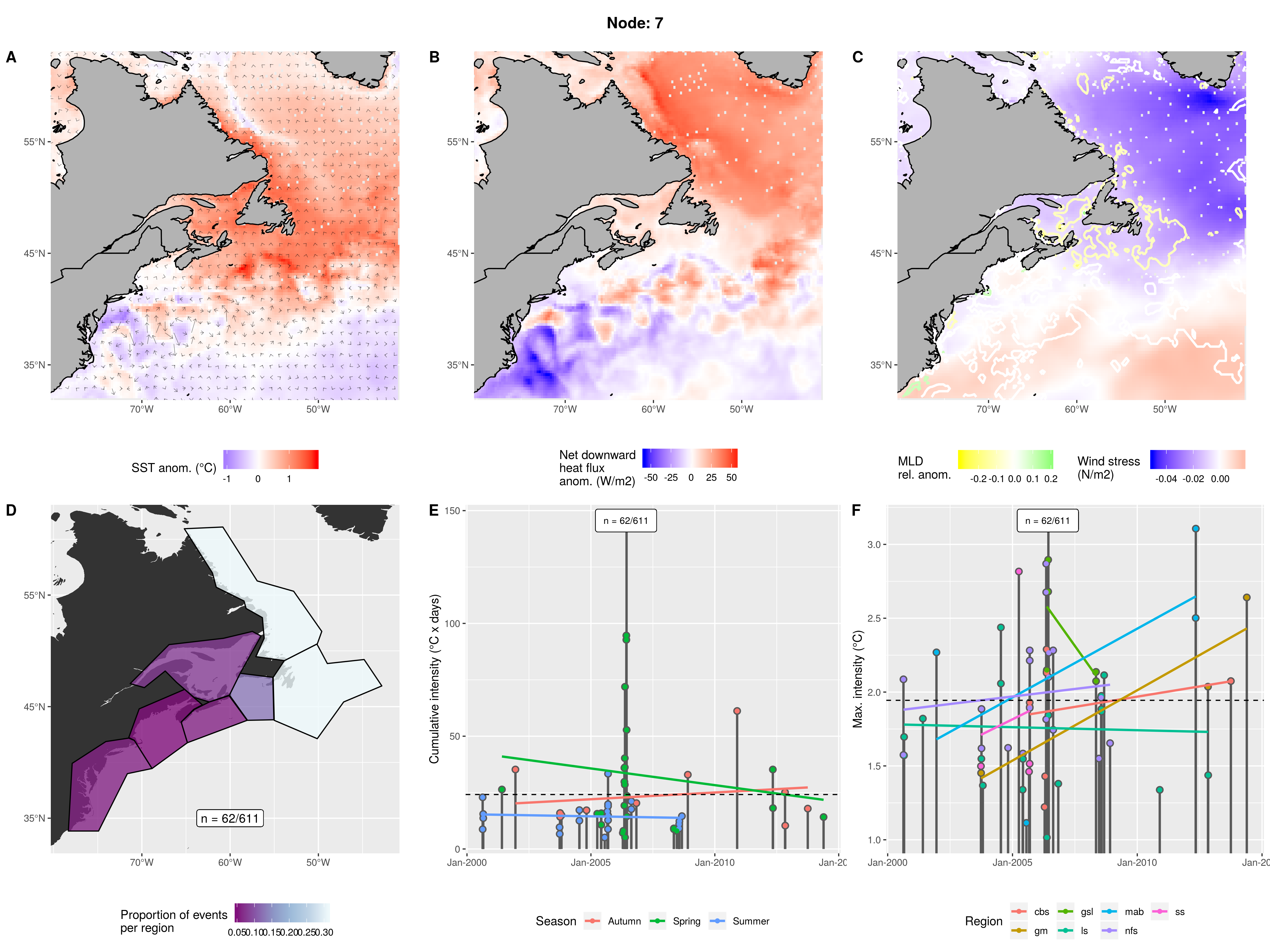
Warm waters from LS to LC to GSL and a cold GS. Strong downward heat flux over northern waters and negative flux over GS. Shallow northern waters with low wind stress while high stress over GS. Equally high in ls and nfs. A bit in cbs but almost none elsewhere. Spring - Autumn from 2000 - 2014. 2006 was a particularly strong year. Events are overall not particularly large.
Expand here to see past versions of node_7_panels.png:
| Version | Author | Date |
|---|---|---|
| 69e8001 | robwschlegel | 2019-07-09 |
Node 8
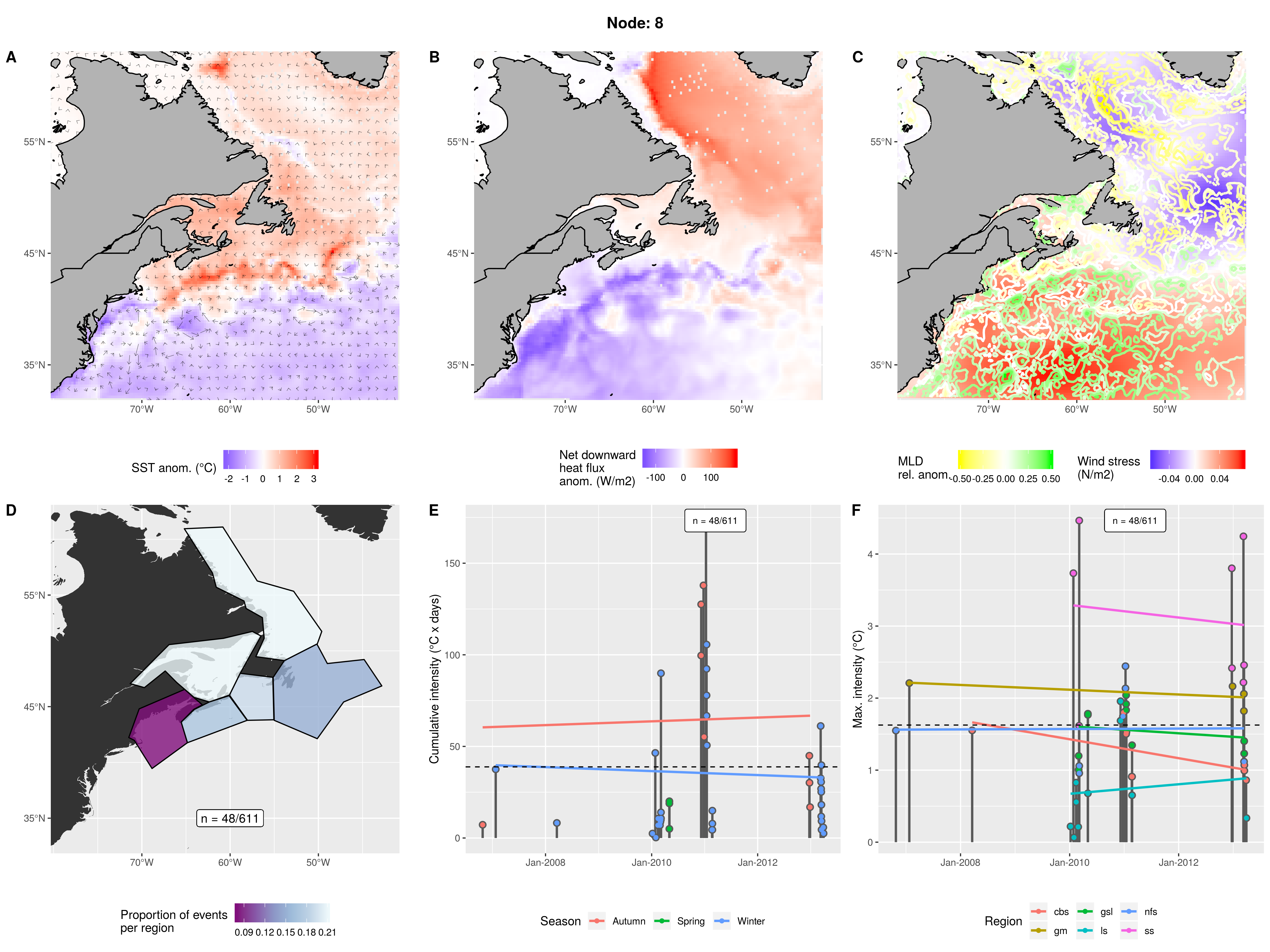
Warm northern waters with a cold GS. Strong positive flux over LS with weaker positive flux over GSL and negative over GS. Very shallow LS and very deep GS. Affects all northern waters but highest in gsl and ls. No events in mab and almost none in gm. Almost always Autumn and Winter from 2006 - 2013. Some more intense events later on with 2010/11 being a larger year.
Expand here to see past versions of node_8_panels.png:
| Version | Author | Date |
|---|---|---|
| 69e8001 | robwschlegel | 2019-07-09 |
Node 9
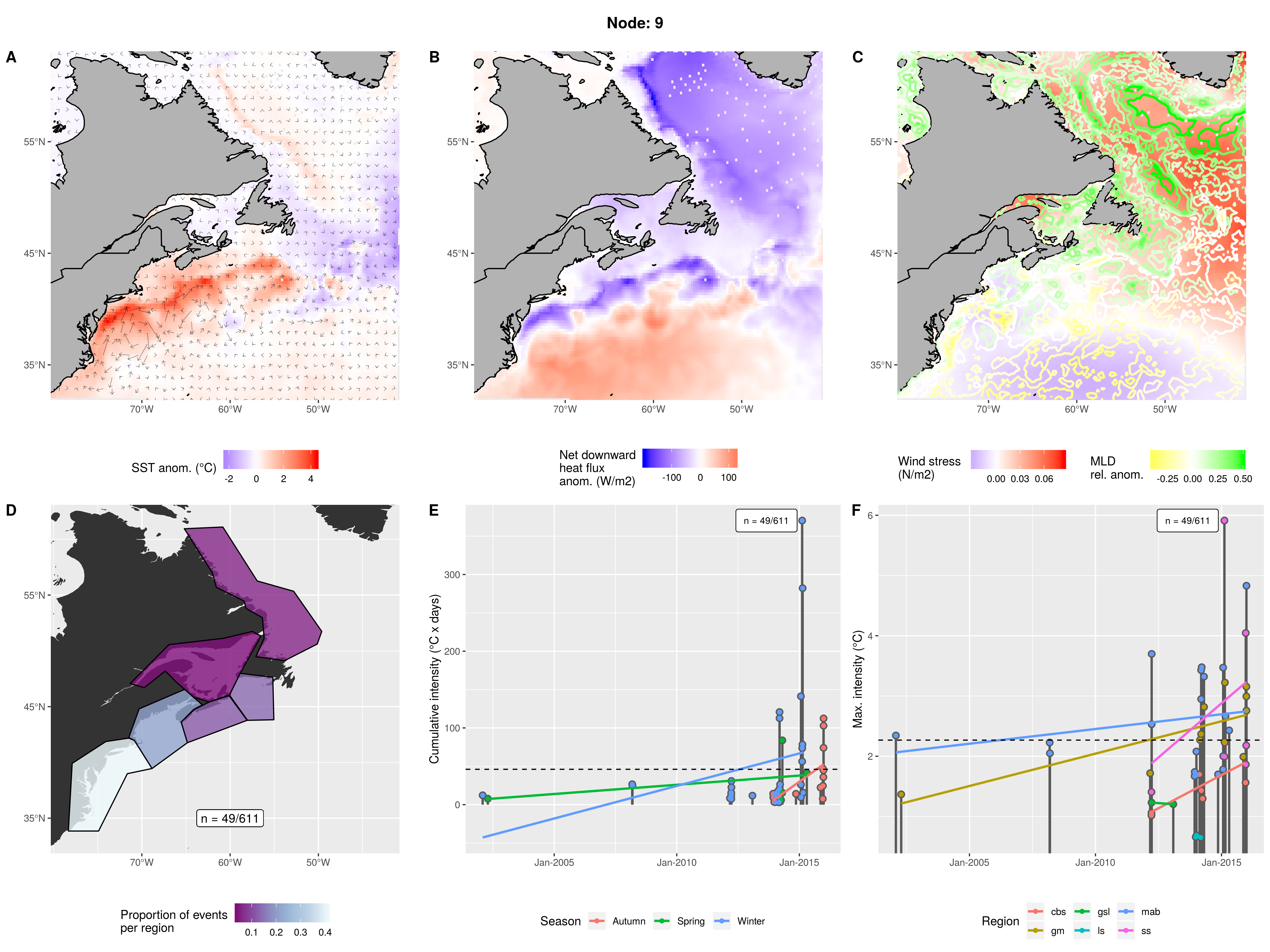
Similar to node 5. Strong nearshore GS pulse. Strong negative flux over LS and GS but positive over the rest of the Atlantic. Very strong wind stress over LS and eastern part of Atlantic, weak over the warm heat flux area of the Atlantic. Extremely deep LS and shallow GS. Occurred over 2002 - 2016 for winter and spring, events began occurring in Autumn from 2013. Evens becoming rather intense as time progresses with some massive ones. Increasing in intensity in most regions.
Expand here to see past versions of node_9_panels.png:
| Version | Author | Date |
|---|---|---|
| 69e8001 | robwschlegel | 2019-07-09 |
Node 10
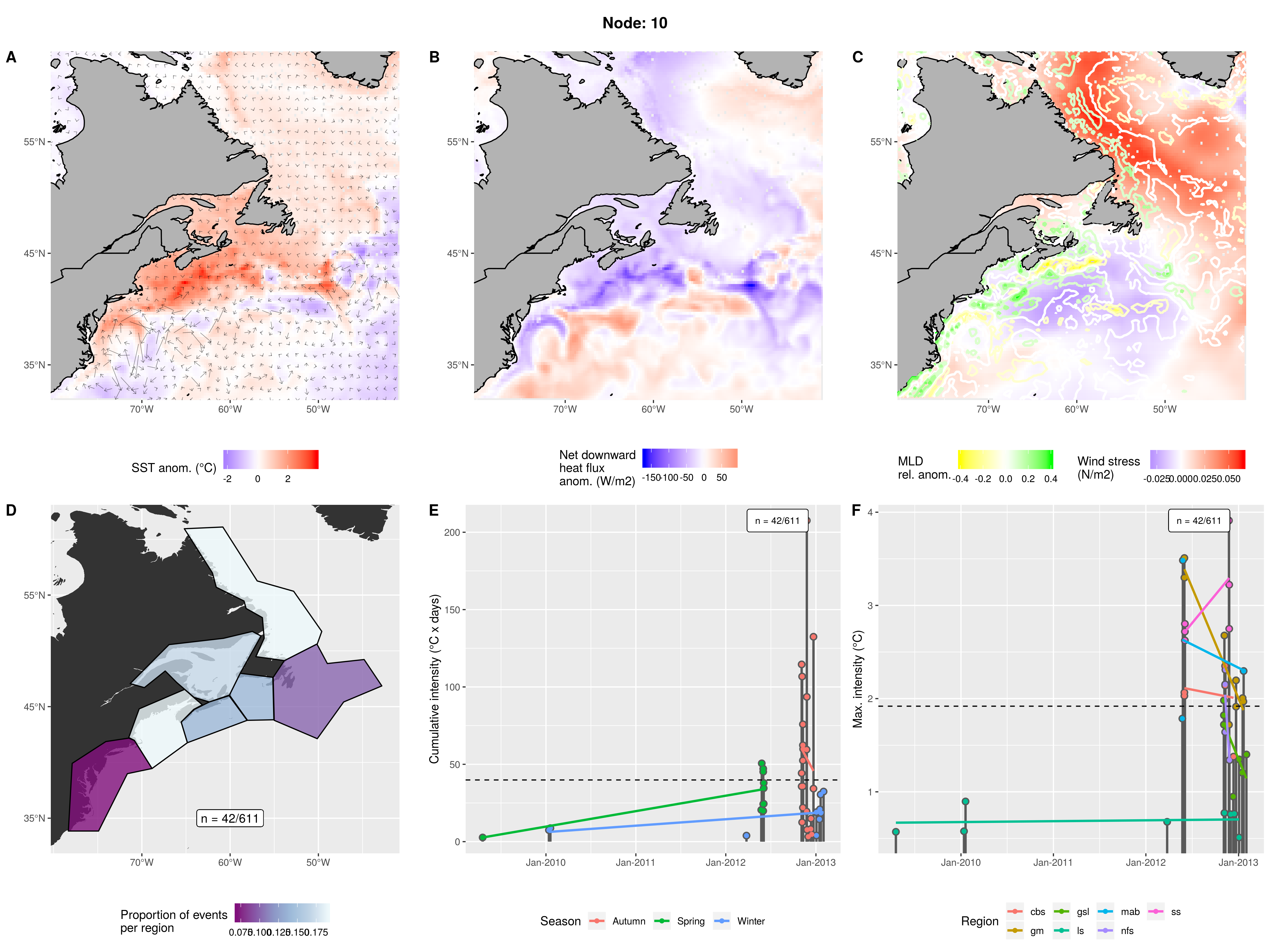
Very unstable mostly cold GS with warm GM and SS waters. Negative heat flux into shelf waters and positive into GS. High wind stress over LS and low over shelf waters. Deep GS and GM waters but shallow over SS. Spread out over most regions with fewest events in mab and nfs. A few tiny events from 2009 - 2011 but really got going from 2012 - 2013. Spring of 2013 was small while Autumn/WInter of 2012/13 was noteworthy.
Expand here to see past versions of node_10_panels.png:
| Version | Author | Date |
|---|---|---|
| 69e8001 | robwschlegel | 2019-07-09 |
Node 11
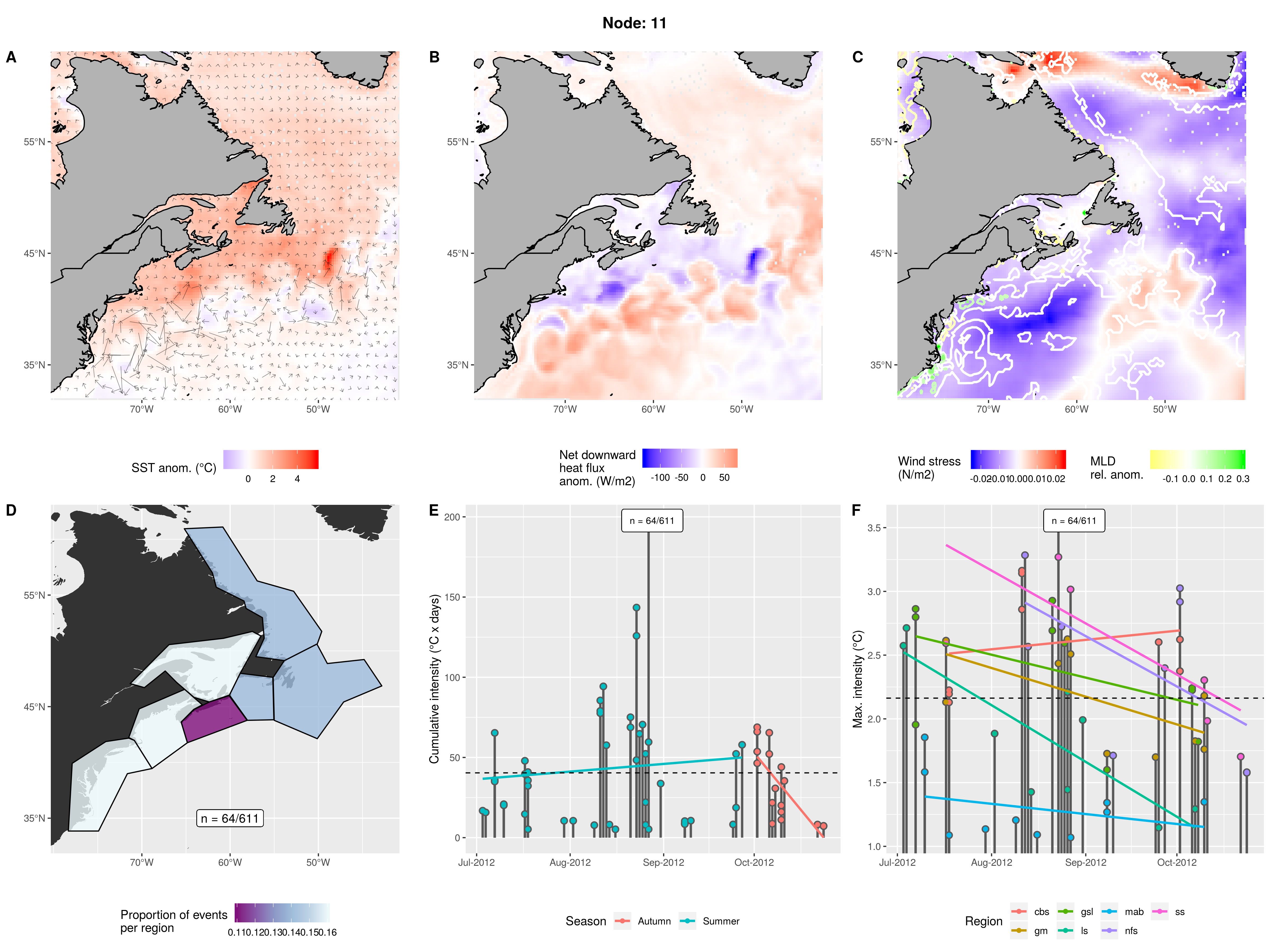
Energetic but normal temperature GS with warm inshore waters and slightly warm LS. Positive heat flux into GS and LS but negative into inshore waters. High wind stress above LS and a bit over central AO, but negative everywhere else. Very deep mixed layer next to coast in MAB but relatively normal everywhere else. Relatively equivalent occurrence in all regions. Occurred only from July - October, 2012. A few decent sized events. Mean max intensity is decent.
Expand here to see past versions of node_11_panels.png:
| Version | Author | Date |
|---|---|---|
| 69e8001 | robwschlegel | 2019-07-09 |
Node 12
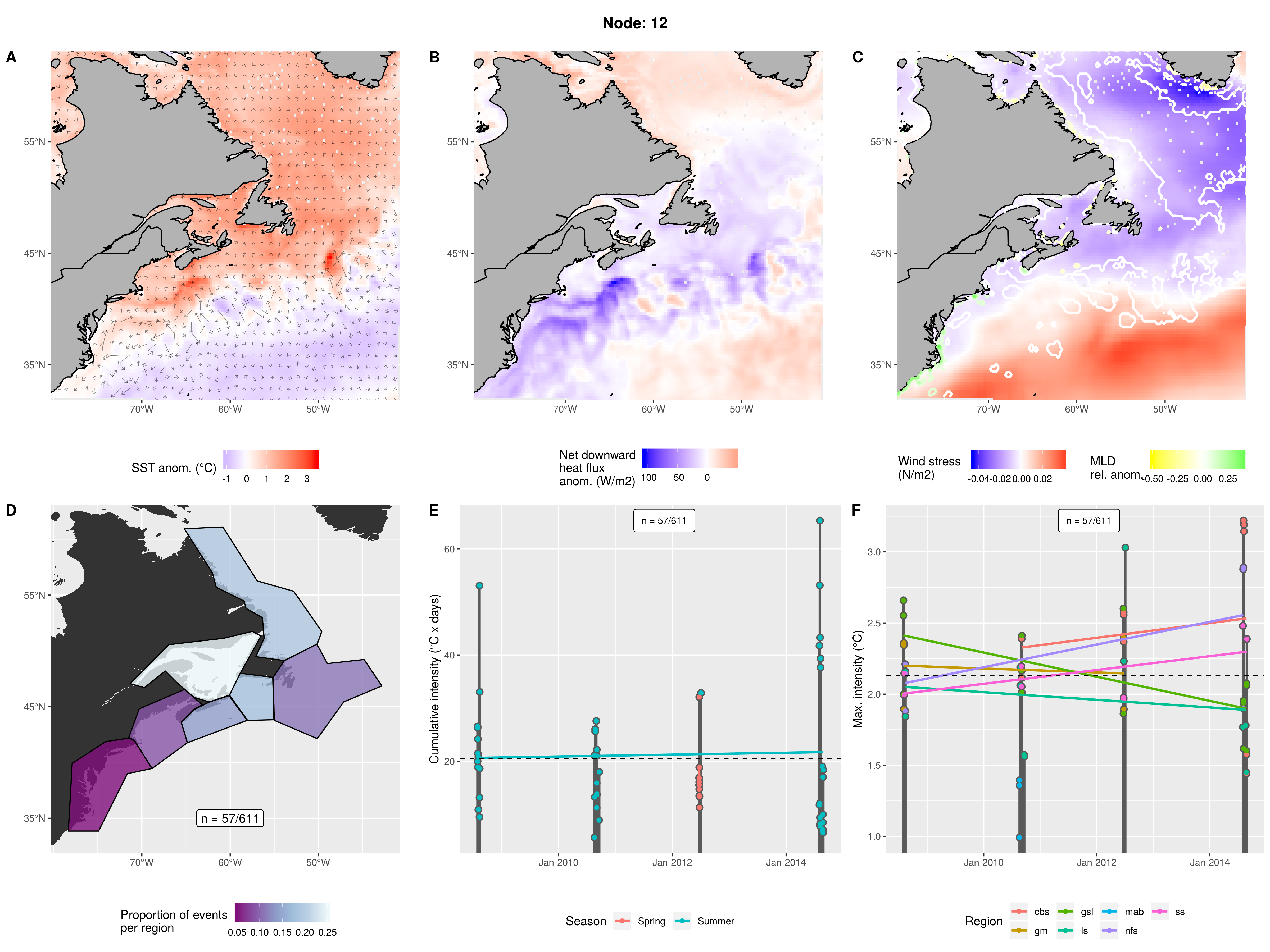
Warm inshore and LS waters with cold GS and AO. GS is moving fast and consistent. Negative heatflux into GS and inshore waters, slightly positive into LS and AO. High wind stress over GS and AO, negative over inshore waters and LS. Very deep mixed layer along coast in mab and very shallow along coast in ls. Mostly events occurring in gsl, but also in other northern areas. Occurred every even year from 2008 to 2014 from ~June - September. Relatively small (short) events but with decent max intensities.
Expand here to see past versions of node_12_panels.png:
| Version | Author | Date |
|---|---|---|
| 69e8001 | robwschlegel | 2019-07-09 |
References
Session information
R version 3.6.1 (2019-07-05)
Platform: x86_64-pc-linux-gnu (64-bit)
Running under: Ubuntu 16.04.5 LTS

Matrix products: default
BLAS:   /usr/lib/openblas-base/libblas.so.3
LAPACK: /usr/lib/libopenblasp-r0.2.18.so

locale:
 [1] LC_CTYPE=en_CA.UTF-8       LC_NUMERIC=C
 [3] LC_TIME=en_CA.UTF-8        LC_COLLATE=en_CA.UTF-8
 [5] LC_MONETARY=en_CA.UTF-8    LC_MESSAGES=en_CA.UTF-8
 [7] LC_PAPER=en_CA.UTF-8       LC_NAME=C
 [9] LC_ADDRESS=C               LC_TELEPHONE=C
[11] LC_MEASUREMENT=en_CA.UTF-8 LC_IDENTIFICATION=C

attached base packages:
[1] stats     graphics  grDevices utils     datasets  methods   base

loaded via a namespace (and not attached):
 [1] workflowr_1.1.1   Rcpp_0.12.18      digest_0.6.16
 [4] rprojroot_1.3-2   R.methodsS3_1.7.1 backports_1.1.2
 [7] git2r_0.23.0      magrittr_1.5      evaluate_0.11
[10] highr_0.7         stringi_1.2.4     whisker_0.3-2
[13] R.oo_1.22.0       R.utils_2.7.0     rmarkdown_1.10
[16] tools_3.6.1       stringr_1.3.1     yaml_2.2.0
[19] compiler_3.6.1    htmltools_0.3.6   knitr_1.20
This reproducible R Markdown analysis was created with workflowr 1.1.1