Acute BDL mouse model
Last updated: 2021-02-27
Checks: 7 0
Knit directory: liver-disease-atlas/
This reproducible R Markdown analysis was created with workflowr (version 1.6.2). The Checks tab describes the reproducibility checks that were applied when the results were created. The Past versions tab lists the development history.
Great! Since the R Markdown file has been committed to the Git repository, you know the exact version of the code that produced these results.
Great job! The global environment was empty. Objects defined in the global environment can affect the analysis in your R Markdown file in unknown ways. For reproduciblity it’s best to always run the code in an empty environment.
The command set.seed(20201218) was run prior to running the code in the R Markdown file. Setting a seed ensures that any results that rely on randomness, e.g. subsampling or permutations, are reproducible.
Great job! Recording the operating system, R version, and package versions is critical for reproducibility.
Nice! There were no cached chunks for this analysis, so you can be confident that you successfully produced the results during this run.
Great job! Using relative paths to the files within your workflowr project makes it easier to run your code on other machines.
Great! You are using Git for version control. Tracking code development and connecting the code version to the results is critical for reproducibility.
The results in this page were generated with repository version 40203d5. See the Past versions tab to see a history of the changes made to the R Markdown and HTML files.
Note that you need to be careful to ensure that all relevant files for the analysis have been committed to Git prior to generating the results (you can use wflow_publish or wflow_git_commit). workflowr only checks the R Markdown file, but you know if there are other scripts or data files that it depends on. Below is the status of the Git repository when the results were generated:
Ignored files:
    Ignored:    .DS_Store
    Ignored:    .Rhistory
    Ignored:    .Rproj.user/
    Ignored:    analysis/human-diehl-nafld_cache/
    Ignored:    analysis/human-hampe13-nash_cache/
    Ignored:    analysis/human-hampe14-misc_cache/
    Ignored:    analysis/human-hoang-nafld_cache/
    Ignored:    analysis/human-ramnath-fibrosis_cache/
    Ignored:    analysis/meta-chronic-vs-acute_cache/
    Ignored:    analysis/meta-mouse-vs-human_cache/
    Ignored:    analysis/mouse-acute-apap_cache/
    Ignored:    analysis/mouse-acute-ccl4_cache/
    Ignored:    analysis/mouse-acute-lps_cache/
    Ignored:    analysis/mouse-acute-ph_cache/
    Ignored:    analysis/mouse-acute-tunicamycin_cache/
    Ignored:    analysis/mouse-chronic-ccl4_cache/
    Ignored:    analysis/plot-acute-apap_cache/
    Ignored:    analysis/plot-acute-bdl_cache/
    Ignored:    analysis/plot-acute-ccl4_cache/
    Ignored:    analysis/plot-acute-ph_cache/
    Ignored:    analysis/plot-chronic-ccl4_cache/
    Ignored:    analysis/plot-chronic-vs-acute_cache/
    Ignored:    analysis/plot-mouse-vs-human_cache/
    Ignored:    analysis/plot-precision-recall_cache/
    Ignored:    analysis/plot-study-overview_cache/
    Ignored:    analysis/plot-teufel-integration_cache/
    Ignored:    analysis/save-tables_cache/
    Ignored:    code/.DS_Store
    Ignored:    code/README.html
    Ignored:    code/meta-mouse-vs-human/.DS_Store
    Ignored:    data.zip
    Ignored:    data/.DS_Store
    Ignored:    data/annotation/
    Ignored:    data/human-diehl-nafld/
    Ignored:    data/human-hampe13-nash/
    Ignored:    data/human-hampe14-misc/
    Ignored:    data/human-hoang-nafld/
    Ignored:    data/human-ramnath-fibrosis/
    Ignored:    data/meta-chronic-vs-acute/
    Ignored:    data/meta-mouse-vs-human/
    Ignored:    data/mouse-acute-apap/
    Ignored:    data/mouse-acute-bdl/
    Ignored:    data/mouse-acute-ccl4/
    Ignored:    data/mouse-acute-lps/
    Ignored:    data/mouse-acute-ph/
    Ignored:    data/mouse-acute-tunicamycin/
    Ignored:    data/mouse-chronic-ccl4/
    Ignored:    external_software/.DS_Store
    Ignored:    external_software/README.html
    Ignored:    external_software/stem/.DS_Store
    Ignored:    figures/
    Ignored:    geo_submission/
    Ignored:    output/.DS_Store
    Ignored:    output/README.html
    Ignored:    output/human-diehl-nafld/
    Ignored:    output/human-hampe13-nash/
    Ignored:    output/human-hampe14-misc/
    Ignored:    output/human-hoang-nafld/
    Ignored:    output/human-ramnath-fibrosis/
    Ignored:    output/meta-chronic-vs-acute/
    Ignored:    output/meta-mouse-vs-human/
    Ignored:    output/mouse-acute-apap/
    Ignored:    output/mouse-acute-bdl/
    Ignored:    output/mouse-acute-ccl4/
    Ignored:    output/mouse-acute-lps/
    Ignored:    output/mouse-acute-ph/
    Ignored:    output/mouse-acute-tunicamycin/
    Ignored:    output/mouse-chronic-ccl4/
    Ignored:    renv/library/
    Ignored:    renv/staging/
    Ignored:    tables/
Note that any generated files, e.g. HTML, png, CSS, etc., are not included in this status report because it is ok for generated content to have uncommitted changes.
These are the previous versions of the repository in which changes were made to the R Markdown (analysis/mouse-acute-bdl.Rmd) and HTML (docs/mouse-acute-bdl.html) files. If you’ve configured a remote Git repository (see ?wflow_git_remote), click on the hyperlinks in the table below to view the files as they were in that past version.
| File | Version | Author | Date | Message |
|---|---|---|---|---|
| Rmd | 40203d5 | christianholland | 2021-02-27 | wflow_publish("analysis/*", delete_cache = TRUE) |
| html | 9c62197 | christianholland | 2021-01-07 | Build site. |
| html | 067c933 | christianholland | 2020-12-23 | Build site. |
| Rmd | d4f78fa | christianholland | 2020-12-23 | wflow_publish("analysis/*.Rmd", delete_cache = T) |
| html | 8a9b7bf | christianholland | 2020-12-20 | Build site. |
| html | e22a40b | christianholland | 2020-12-20 | Build site. |
| html | bea437a | christianholland | 2020-12-20 | Build site. |
| Rmd | c78e883 | christianholland | 2020-12-20 | stem characterization |
| html | af38450 | christianholland | 2020-12-19 | Build site. |
| Rmd | 78a25d5 | christianholland | 2020-12-19 | minor changes |
| html | 3a3aef8 | christianholland | 2020-12-19 | Build site. |
| Rmd | 0a70042 | christianholland | 2020-12-19 | added acute bdl study |
Introduction
Here we analysis a mouse model of BDL (Bile Duct Ligation) induced acute liver damage. The transcriptomic profiles were measured at 4 different time points ranging from 1 day to 21 days. For the time points 1, 3, and 7 days time-matched controls are available.
Libraries and sources
These libraries and sources are used for this analysis.
library(mogene20sttranscriptcluster.db)

library(tidyverse)
library(tidylog)
library(here)

library(oligo)
library(annotate)
library(limma)
library(biobroom)
library(progeny)
library(dorothea)

library(janitor)
library(msigdf) # remotes::install_github("ToledoEM/msigdf@v7.1")

library(AachenColorPalette)
library(cowplot)
library(lemon)
library(patchwork)

options("tidylog.display" = list(print))
source(here("code/utils-microarray.R"))
source(here("code/utils-utils.R"))
source(here("code/utils-plots.R"))
Definition of global variables that are used throughout this analysis.
# i/o
data_path <- "data/mouse-acute-bdl"
output_path <- "output/mouse-acute-bdl"

# graphical parameters
# fontsize
fz <- 9
Data processing
Load .CEL files and quality control
The array quality is controlled based on the relative log expression values (RLE) and the normalized unscaled standard errors (NUSE).
# load cel files and check quality
platforms <- readRDS(here("data/annotation/platforms.rds"))
raw_eset <- list.celfiles(here(data_path), listGzipped = T, full.names = T) %>%
  read.celfiles() %>%
  ma_qc() # Discarding in total 1 arrays: 489-944wt 1d Sham_(MoGene-2_0-st).CEL
#> Reading in : /Users/cholland/Google Drive/Projects/liver-disease-atlas/data/mouse-acute-bdl/489-678wt 7d Sham_(MoGene-2_0-st).CEL
#> Reading in : /Users/cholland/Google Drive/Projects/liver-disease-atlas/data/mouse-acute-bdl/489-690wt 7d Sham_(MoGene-2_0-st).CEL
#> Reading in : /Users/cholland/Google Drive/Projects/liver-disease-atlas/data/mouse-acute-bdl/489-691wt 7d Sham_(MoGene-2_0-st).CEL
#> Reading in : /Users/cholland/Google Drive/Projects/liver-disease-atlas/data/mouse-acute-bdl/489-697wt 7d Sham_(MoGene-2_0-st).CEL
#> Reading in : /Users/cholland/Google Drive/Projects/liver-disease-atlas/data/mouse-acute-bdl/489-709wt 7d BDL_(MoGene-2_0-st).CEL
#> Reading in : /Users/cholland/Google Drive/Projects/liver-disease-atlas/data/mouse-acute-bdl/489-713wt 7d BDL_(MoGene-2_0-st).CEL
#> Reading in : /Users/cholland/Google Drive/Projects/liver-disease-atlas/data/mouse-acute-bdl/489-714wt 7d BDL_(MoGene-2_0-st).CEL
#> Reading in : /Users/cholland/Google Drive/Projects/liver-disease-atlas/data/mouse-acute-bdl/489-740wt 3d BDL_(MoGene-2_0-st).CEL
#> Reading in : /Users/cholland/Google Drive/Projects/liver-disease-atlas/data/mouse-acute-bdl/489-741wt 3d BDL_(MoGene-2_0-st).CEL
#> Reading in : /Users/cholland/Google Drive/Projects/liver-disease-atlas/data/mouse-acute-bdl/489-744wt 7d BDL_(MoGene-2_0-st).CEL
#> Reading in : /Users/cholland/Google Drive/Projects/liver-disease-atlas/data/mouse-acute-bdl/489-750wt 7d BDL_(MoGene-2_0-st).CEL
#> Reading in : /Users/cholland/Google Drive/Projects/liver-disease-atlas/data/mouse-acute-bdl/489-776wt 3d BDL_(MoGene-2_0-st).CEL
#> Reading in : /Users/cholland/Google Drive/Projects/liver-disease-atlas/data/mouse-acute-bdl/489-778wt 3d BDL_(MoGene-2_0-st).CEL
#> Reading in : /Users/cholland/Google Drive/Projects/liver-disease-atlas/data/mouse-acute-bdl/489-806wt 21d BDL_(MoGene-2_0-st).CEL
#> Reading in : /Users/cholland/Google Drive/Projects/liver-disease-atlas/data/mouse-acute-bdl/489-853wt 21d BDL_(MoGene-2_0-st).CEL
#> Reading in : /Users/cholland/Google Drive/Projects/liver-disease-atlas/data/mouse-acute-bdl/489-855wt 21d BDL_(MoGene-2_0-st).CEL
#> Reading in : /Users/cholland/Google Drive/Projects/liver-disease-atlas/data/mouse-acute-bdl/489-884wt 21d BDL_(MoGene-2_0-st).CEL
#> Reading in : /Users/cholland/Google Drive/Projects/liver-disease-atlas/data/mouse-acute-bdl/489-886wt 21d BDL_(MoGene-2_0-st).CEL
#> Reading in : /Users/cholland/Google Drive/Projects/liver-disease-atlas/data/mouse-acute-bdl/489-911wt 3d BDL_(MoGene-2_0-st).CEL
#> Reading in : /Users/cholland/Google Drive/Projects/liver-disease-atlas/data/mouse-acute-bdl/489-913wt 3d Sham_(MoGene-2_0-st).CEL
#> Reading in : /Users/cholland/Google Drive/Projects/liver-disease-atlas/data/mouse-acute-bdl/489-927wt 3d Sham_(MoGene-2_0-st).CEL
#> Reading in : /Users/cholland/Google Drive/Projects/liver-disease-atlas/data/mouse-acute-bdl/489-928wt 1d BDL_(MoGene-2_0-st).CEL
#> Reading in : /Users/cholland/Google Drive/Projects/liver-disease-atlas/data/mouse-acute-bdl/489-931wt 1d Sham_(MoGene-2_0-st).CEL
#> Reading in : /Users/cholland/Google Drive/Projects/liver-disease-atlas/data/mouse-acute-bdl/489-939wt 1d BDL_(MoGene-2_0-st).CEL
#> Reading in : /Users/cholland/Google Drive/Projects/liver-disease-atlas/data/mouse-acute-bdl/489-940wt 1d BDL_(MoGene-2_0-st).CEL
#> Reading in : /Users/cholland/Google Drive/Projects/liver-disease-atlas/data/mouse-acute-bdl/489-944wt 1d Sham_(MoGene-2_0-st).CEL
#> Reading in : /Users/cholland/Google Drive/Projects/liver-disease-atlas/data/mouse-acute-bdl/489-945wt 1d BDL_(MoGene-2_0-st).CEL
#> Reading in : /Users/cholland/Google Drive/Projects/liver-disease-atlas/data/mouse-acute-bdl/489-956wt 1d BDL_(MoGene-2_0-st).CEL
#> Reading in : /Users/cholland/Google Drive/Projects/liver-disease-atlas/data/mouse-acute-bdl/489-957wt 1d Sham_(MoGene-2_0-st).CEL
#> Reading in : /Users/cholland/Google Drive/Projects/liver-disease-atlas/data/mouse-acute-bdl/489-960wt 1d Sham_(MoGene-2_0-st).CEL
Normalization and probe annotation
Probe intensities are normalized with the rma() function. Probes are annotated with MGI symbols.
eset <- rma(raw_eset)
#> Background correcting
#> Normalizing
#> Calculating Expression

# annotate microarray probes with mgi symbols
expr <- ma_annotate(eset, platforms)

# save normalized expression
saveRDS(expr, here(output_path, "normalized_expression.rds"))
Build meta data
Meta information are parsed from the sample names.
# build meta data
meta <- colnames(expr) %>%
  enframe(name = NULL, value = "sample") %>%
  separate(sample, into = c(
    "tmp1", "mouse", "time", "treatment",
    "tmp"
  ), remove = F, extra = "merge") %>%
  dplyr::select(-starts_with("tmp")) %>%
  mutate(
    time = ordered(parse_number(time)),
    mouse = str_remove(mouse, "wt"),
    treatment = factor(str_to_lower(treatment), levels = c("sham", "bdl")),
    group = str_c(treatment, str_c(time, "d"), sep = "_")
  ) %>%
  mutate(group = factor(group, levels = c(
    "sham_1d", "bdl_1d", "sham_3d",
    "bdl_3d", "sham_7d", "bdl_7d",
    "bdl_21d"
  )))
#> mutate: changed 29 values (100%) of 'mouse' (0 new NA)
#>         converted 'time' from character to ordered factor (0 new NA)
#>         converted 'treatment' from character to factor (0 new NA)
#>         new variable 'group' (character) with 7 unique values and 0% NA
#> mutate: converted 'group' from character to factor (0 new NA)

# save meta data
saveRDS(meta, here(output_path, "meta_data.rds"))
Exploratory analysis
PCA of normalized data
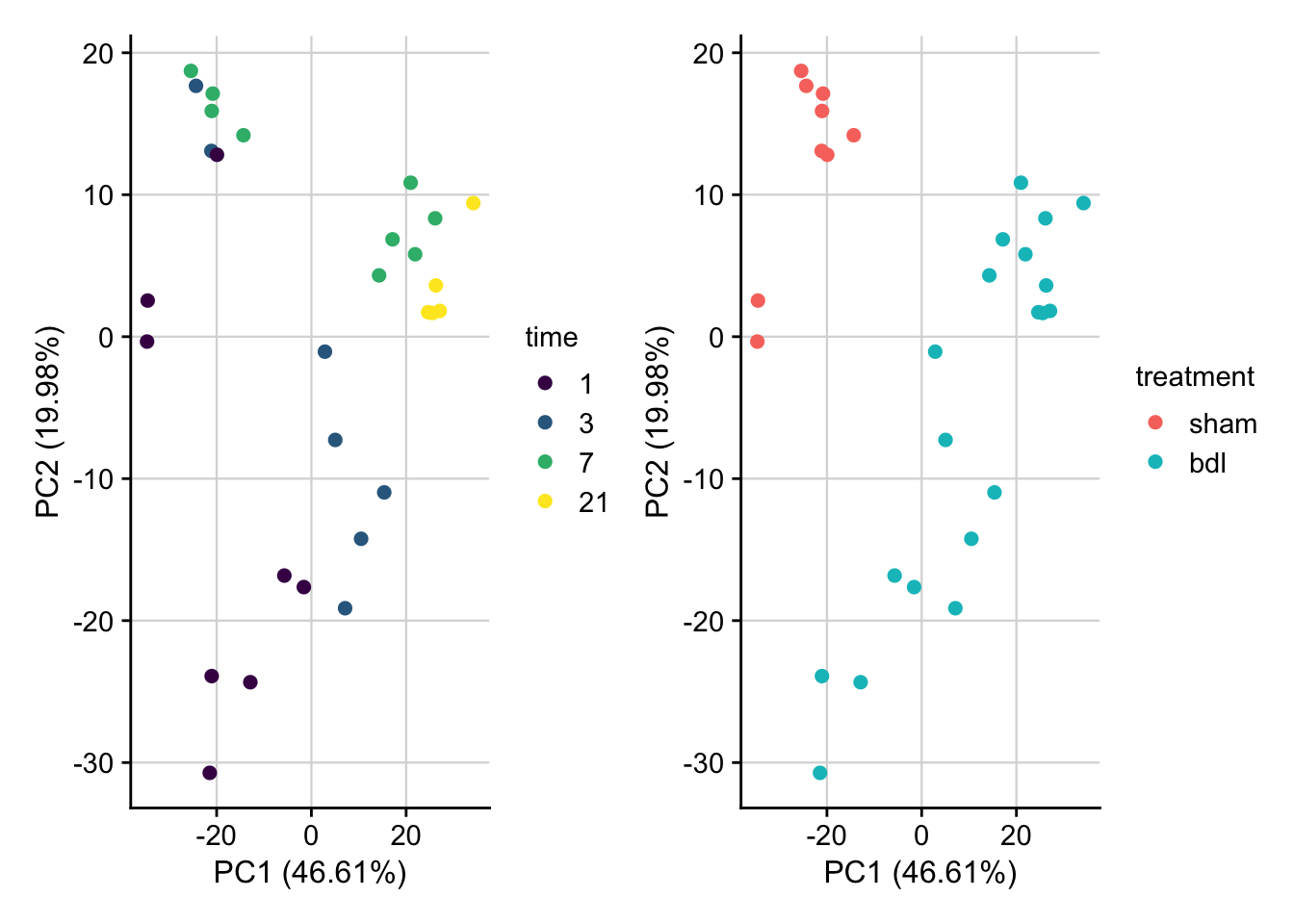
PCA plot of normalized expression data contextualized based on the time point and treatment. Only the top 1000 most variable genes are used as features.
expr <- readRDS(here(output_path, "normalized_expression.rds"))
meta <- readRDS(here(output_path, "meta_data.rds"))

pca_result <- do_pca(expr, meta, top_n_var_genes = 1000)
#> left_join: added 4 columns (mouse, time, treatment, group)
#>            > rows only in x    0
#>            > rows only in y  ( 0)
#>            > matched rows     29
#>            >                 ====
#>            > rows total       29

saveRDS(pca_result, here(output_path, "pca_result.rds"))

plot_pca(pca_result, feature = "time") +
  plot_pca(pca_result, feature = "treatment") &
  my_theme()
Differential gene expression analysis
Running limma
Differential gene expression analysis via limma with the aim to identify the effect of BDL for the different time points.
# load expression and meta data
expr <- readRDS(here(output_path, "normalized_expression.rds"))
meta <- readRDS(here(output_path, "meta_data.rds"))

stopifnot(colnames(expr) == meta$sample)

# build design matrix
design <- model.matrix(~ 0 + group, data = meta)
rownames(design) <- meta$sample
colnames(design) <- levels(meta$group)

# define contrasts
contrasts <- makeContrasts(
  # time matched effect of bdl
  bdl_vs_sham_1d = bdl_1d - sham_1d,
  bdl_vs_sham_3d = bdl_3d - sham_3d,
  bdl_vs_sham_7d = bdl_7d - sham_7d,
  bdl_vs_sham_21d = bdl_21d - (sham_1d + sham_3d + sham_7d) / 3,

  # pair-wise bdl comparison
  bdl_3d_vs_1d = bdl_3d - bdl_1d,
  bdl_7d_vs_1d = bdl_7d - bdl_1d,
  bdl_21d_vs_1d = bdl_21d - bdl_1d,
  bdl_7d_vs_3d = bdl_7d - bdl_3d,
  bdl_21d_vs_3d = bdl_21d - bdl_3d,
  bdl_21d_vs_7d = bdl_21d - bdl_7d,

  # pair-wise sham comparison
  sham_3d_vs_1d = sham_3d - sham_1d,
  sham_7d_vs_1d = sham_7d - sham_1d,
  sham_7d_vs_3d = sham_7d - sham_3d,

  levels = design
)

limma_result <- run_limma(expr, design, contrasts) %>%
  assign_deg()
#> select: renamed 3 variables (contrast, logFC, pval) and dropped one variable
#> group_by: one grouping variable (contrast)
#> mutate (grouped): new variable 'fdr' (double) with 133,423 unique values and 0% NA
#> ungroup: no grouping variables
#> mutate: new variable 'regulation' (character) with 3 unique values and 0% NA
#> mutate: converted 'regulation' from character to factor (0 new NA)

deg_df <- limma_result %>%
  mutate(contrast = factor(contrast, levels = c(
    "bdl_vs_sham_1d", "bdl_vs_sham_3d", "bdl_vs_sham_7d", "bdl_vs_sham_21d",
    "bdl_3d_vs_1d",
    "bdl_7d_vs_1d", "bdl_21d_vs_1d", "bdl_7d_vs_3d", "bdl_21d_vs_3d",
    "bdl_21d_vs_7d", "sham_3d_vs_1d", "sham_7d_vs_1d", "sham_7d_vs_3d"
  ))) %>%
  mutate(contrast_reference = case_when(
    str_detect(contrast, "vs_sham") ~ "bdl",
    str_detect(contrast, "bdl_\\d*") ~ "pairwise_bdl",
    str_detect(contrast, "sham_\\d*") ~ "pairwise_sham"
  ))
#> mutate: changed 0 values (0%) of 'contrast' (0 new NA)
#> mutate: new variable 'contrast_reference' (character) with 3 unique values and 0% NA

saveRDS(deg_df, here(output_path, "limma_result.rds"))
Volcano plots
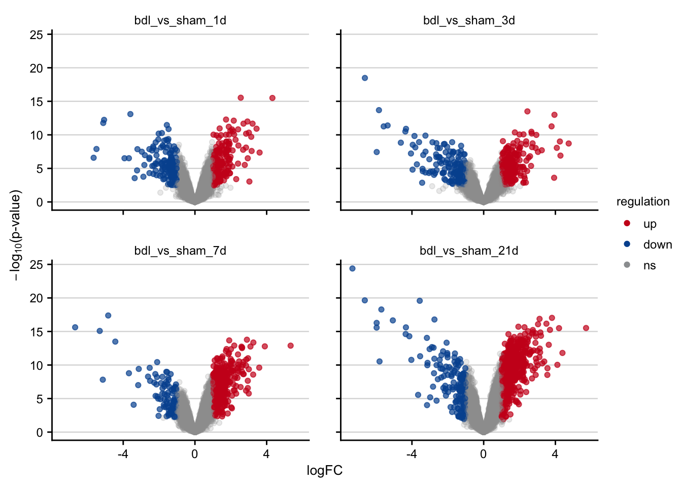
Volcano plots visualizing the effect of BDL on gene expression.
df <- readRDS(here(output_path, "limma_result.rds"))

df %>%
  filter(contrast_reference == "bdl") %>%
  plot_volcano() +
  my_theme(grid = "y", fsize = fz)
#> filter: removed 215,676 rows (69%), 95,856 rows remaining
#> rename: renamed one variable (p)
Time series clustering
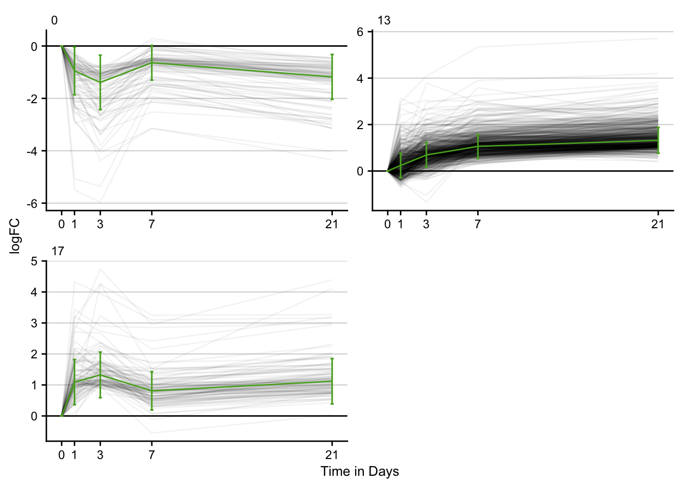
Gene expression trajectories are clustered using the STEM software. The cluster algorithm is described here.
Prepare input
# prepare input for stem analysis
df <- readRDS(here(output_path, "limma_result.rds"))

stem_inputs <- df %>%
  mutate(class = str_c("Day ", parse_number(as.character(contrast)))) %>%
  mutate(class = factor(class, levels = unique(.$class))) %>%
  select(gene, class, logFC, contrast_reference)
#> mutate: new variable 'class' (character) with 4 unique values and 0% NA
#> mutate: converted 'class' from character to factor (0 new NA)
#> select: dropped 5 variables (contrast, statistic, pval, fdr, regulation)

stem_inputs %>%
  filter(contrast_reference == "bdl") %>%
  select(-contrast_reference) %>%
  pivot_wider(names_from = class, values_from = logFC) %>%
  write_delim(here(output_path, "stem/input/bdl.txt"), delim = "\t")
#> filter: removed 215,676 rows (69%), 95,856 rows remaining
#> select: dropped one variable (contrast_reference)
#> pivot_wider: reorganized (class, logFC) into (Day 1, Day 3, Day 7, Day 21) [was 95856x3, now 23964x5]
Run STEM
STEM is implemented in Java. The .jar file is called from R. Only significant time series clusters are visualized.
# execute stem
stem_res <- run_stem(file.path(output_path, "stem"), clear_output = T)
#> distinct: no rows removed
#> mutate: new variable 'gene' (character) with 23,964 unique values and 0% NA
#> distinct: no rows removed
#> mutate: new variable 'key' (character) with one unique value and 0% NA
#> select: dropped one variable (spot)
#> gather: reorganized (x0, day_1, day_3, day_7, day_21) into (time, value) [was 1557x8, now 7785x5]
#> mutate: converted 'time' from character to double (0 new NA)
#> mutate: new variable 'key' (character) with one unique value and 0% NA
#> select: renamed 4 variables (profile, y_coords, size, p) and dropped 2 variables
#> inner_join: added 3 columns (y_coords, size, p)
#>             > rows only in x  (    0)
#>             > rows only in y  (    0)
#>             > matched rows     7,785
#>             >                 =======
#>             > rows total       7,785
#> inner_join: added one column (symbol)
#>             > rows only in x  (     0)
#>             > rows only in y  (22,407)
#>             > matched rows      7,785
#>             >                 ========
#>             > rows total        7,785
#> transmute: dropped one variable (symbol)
#>            changed 7,685 values (99%) of 'gene' (0 new NA)

saveRDS(stem_res, here(output_path, "stem_result.rds"))

stem_res %>%
  filter(p <= 0.05) %>%
  filter(key == "bdl") %>%
  distinct() %>%
  plot_stem_profiles(model_profile = F, ncol = 2) +
  labs(x = "Time in Days", y = "logFC") +
  my_theme(grid = "y", fsize = fz)
#> filter: removed 3,485 rows (45%), 4,300 rows remaining
#> filter: no rows removed
#> distinct: no rows removed
#> group_by: 4 grouping variables (key, profile, p, time)
#> ungroup: no grouping variables
Cluster characterization
STEM clusters are characterized by GO terms, PROGENy’s pathways and DoRothEA’s TFs. As statistic over-representation analysis is used.
stem_res = readRDS(here(output_path, "stem_result.rds"))

signatures = stem_res %>%
  filter(p <= 0.05) %>%
  distinct(profile, gene, p_profile = p)
#> filter: removed 3,485 rows (45%), 4,300 rows remaining
#> distinct: removed 3,440 rows (80%), 860 rows remaining

genesets = load_genesets() %>%
  filter(confidence %in% c(NA,"A", "B", "C"))
#> filter: removed 2,340,732 rows (80%), 597,560 rows remaining
#> select: renamed one variable (gene) and dropped 2 variables
#> mutate: new variable 'group' (character) with one unique value and 0% NA
#> gather: reorganized (Androgen, EGFR, Estrogen, Hypoxia, JAK-STAT, …) into (geneset, weight) [was 1299x15, now 18186x3]
#> filter: removed 16,785 rows (92%), 1,401 rows remaining
#> select: dropped one variable (weight)
#> mutate: new variable 'group' (character) with one unique value and 0% NA
#> select: renamed 2 variables (geneset, gene) and dropped one variable
#> mutate: new variable 'group' (character) with one unique value and 0% NA
#> filter: removed 396,818 rows (39%), 612,694 rows remaining

ora_res = signatures %>%
  nest(sig = c(-profile)) %>%
  dplyr::mutate(ora = sig %>% map(run_ora,  sets = genesets, min_size = 10,
                           options = list(alternative = "greater"),
                           background_n = 20000)) %>%
  select(-sig) %>%
  unnest(ora)
#> add_count: new variable 'n' (integer) with 643 unique values and 0% NA
#> filter: removed 13,996 rows (2%), 598,698 rows remaining
#> select: dropped one variable (n)
#> mutate: new variable 'contingency_table' (list) with 1,955 unique values and 0% NA
#> mutate: new variable 'stat' (list) with 1,852 unique values and 0% NA
#> group_by: one grouping variable (group)
#> mutate (grouped): new variable 'fdr' (double) with 1,494 unique values and 0% NA
#> ungroup: no grouping variables
#> select: dropped 4 variables (set, conf.low, conf.high, method)
#> add_count: new variable 'n' (integer) with 643 unique values and 0% NA
#> filter: removed 13,996 rows (2%), 598,698 rows remaining
#> select: dropped one variable (n)
#> mutate: new variable 'contingency_table' (list) with 1,209 unique values and 0% NA
#> mutate: new variable 'stat' (list) with 990 unique values and 0% NA
#> group_by: one grouping variable (group)
#> mutate (grouped): new variable 'fdr' (double) with 626 unique values and 0% NA
#> ungroup: no grouping variables
#> select: dropped 4 variables (set, conf.low, conf.high, method)
#> add_count: new variable 'n' (integer) with 643 unique values and 0% NA
#> filter: removed 13,996 rows (2%), 598,698 rows remaining
#> select: dropped one variable (n)
#> mutate: new variable 'contingency_table' (list) with 1,036 unique values and 0% NA
#> mutate: new variable 'stat' (list) with 670 unique values and 0% NA
#> group_by: one grouping variable (group)
#> mutate (grouped): new variable 'fdr' (double) with 343 unique values and 0% NA
#> ungroup: no grouping variables
#> select: dropped 4 variables (set, conf.low, conf.high, method)
#> select: dropped one variable (sig)

saveRDS(ora_res, here(output_path, "stem_characterization.rds"))
Time spend to execute this analysis: 03:57 minutes.
sessionInfo()
#> R version 4.0.2 (2020-06-22)
#> Platform: x86_64-apple-darwin17.0 (64-bit)
#> Running under: macOS Mojave 10.14.5
#>
#> Matrix products: default
#> BLAS:   /Library/Frameworks/R.framework/Versions/4.0/Resources/lib/libRblas.dylib
#> LAPACK: /Library/Frameworks/R.framework/Versions/4.0/Resources/lib/libRlapack.dylib
#>
#> locale:
#> [1] en_US.UTF-8/en_US.UTF-8/en_US.UTF-8/C/en_US.UTF-8/en_US.UTF-8
#>
#> attached base packages:
#> [1] parallel  stats4    stats     graphics  grDevices datasets  utils
#> [8] methods   base
#>
#> other attached packages:
#>  [1] pd.mogene.2.0.st_3.14.1              DBI_1.1.0
#>  [3] RSQLite_2.2.1                        patchwork_1.1.1
#>  [5] lemon_0.4.5                          cowplot_1.1.0
#>  [7] AachenColorPalette_1.1.2             msigdf_7.1
#>  [9] janitor_2.0.1                        dorothea_1.0.1
#> [11] progeny_1.10.0                       biobroom_1.20.0
#> [13] broom_0.7.3                          limma_3.44.3
#> [15] annotate_1.66.0                      XML_3.99-0.5
#> [17] oligo_1.52.1                         Biostrings_2.56.0
#> [19] XVector_0.28.0                       oligoClasses_1.50.4
#> [21] here_1.0.1                           tidylog_1.0.2
#> [23] forcats_0.5.0                        stringr_1.4.0
#> [25] dplyr_1.0.2                          purrr_0.3.4
#> [27] readr_1.4.0                          tidyr_1.1.2
#> [29] tibble_3.0.4                         ggplot2_3.3.2
#> [31] tidyverse_1.3.0                      mogene20sttranscriptcluster.db_8.7.0
#> [33] org.Mm.eg.db_3.11.4                  AnnotationDbi_1.50.3
#> [35] IRanges_2.22.2                       S4Vectors_0.26.1
#> [37] Biobase_2.48.0                       BiocGenerics_0.34.0
#> [39] workflowr_1.6.2
#>
#> loaded via a namespace (and not attached):
#>  [1] colorspace_2.0-0            ellipsis_0.3.1
#>  [3] rprojroot_2.0.2             snakecase_0.11.0
#>  [5] GenomicRanges_1.40.0        fs_1.5.0
#>  [7] rstudioapi_0.13             farver_2.0.3
#>  [9] affyio_1.58.0               ggrepel_0.9.0
#> [11] bit64_4.0.5                 fansi_0.4.1
#> [13] lubridate_1.7.9.2           xml2_1.3.2
#> [15] codetools_0.2-16            splines_4.0.2
#> [17] knitr_1.30                  jsonlite_1.7.2
#> [19] bcellViper_1.24.0           dbplyr_2.0.0
#> [21] BiocManager_1.30.10         compiler_4.0.2
#> [23] httr_1.4.2                  backports_1.2.1
#> [25] assertthat_0.2.1            Matrix_1.2-18
#> [27] cli_2.2.0                   later_1.1.0.1
#> [29] htmltools_0.5.0             tools_4.0.2
#> [31] gtable_0.3.0                glue_1.4.2
#> [33] GenomeInfoDbData_1.2.3      affxparser_1.60.0
#> [35] Rcpp_1.0.5                  cellranger_1.1.0
#> [37] vctrs_0.3.6                 preprocessCore_1.50.0
#> [39] iterators_1.0.13            xfun_0.19
#> [41] rvest_0.3.6                 lifecycle_0.2.0
#> [43] renv_0.12.3                 zlibbioc_1.34.0
#> [45] scales_1.1.1                clisymbols_1.2.0
#> [47] hms_0.5.3                   promises_1.1.1
#> [49] SummarizedExperiment_1.18.2 yaml_2.2.1
#> [51] gridExtra_2.3               memoise_1.1.0
#> [53] stringi_1.5.3               foreach_1.5.1
#> [55] GenomeInfoDb_1.24.2         rlang_0.4.9
#> [57] pkgconfig_2.0.3             bitops_1.0-6
#> [59] matrixStats_0.57.0          evaluate_0.14
#> [61] lattice_0.20-41             labeling_0.4.2
#> [63] bit_4.0.4                   tidyselect_1.1.0
#> [65] plyr_1.8.6                  magrittr_2.0.1
#> [67] R6_2.5.0                    generics_0.1.0
#> [69] DelayedArray_0.14.1         pillar_1.4.7
#> [71] haven_2.3.1                 whisker_0.4
#> [73] withr_2.3.0                 RCurl_1.98-1.2
#> [75] modelr_0.1.8                crayon_1.3.4
#> [77] rmarkdown_2.6               grid_4.0.2
#> [79] readxl_1.3.1                blob_1.2.1
#> [81] git2r_0.27.1                reprex_0.3.0
#> [83] digest_0.6.27               xtable_1.8-4
#> [85] ff_4.0.4                    httpuv_1.5.4
#> [87] munsell_0.5.0               viridisLite_0.3.0