Home
Last updated: 2019-10-23
Checks: 2 0
Knit directory: mr-ash-workflow/
This reproducible R Markdown analysis was created with workflowr (version 1.3.0). The Checks tab describes the reproducibility checks that were applied when the results were created. The Past versions tab lists the development history.
Great! Since the R Markdown file has been committed to the Git repository, you know the exact version of the code that produced these results.
Great! You are using Git for version control. Tracking code development and connecting the code version to the results is critical for reproducibility. The version displayed above was the version of the Git repository at the time these results were generated.
Note that you need to be careful to ensure that all relevant files for the analysis have been committed to Git prior to generating the results (you can use wflow_publish or wflow_git_commit). workflowr only checks the R Markdown file, but you know if there are other scripts or data files that it depends on. Below is the status of the Git repository when the results were generated:
Ignored files:
    Ignored:    .Rhistory
    Ignored:    .Rproj.user/
    Ignored:    ETA_1_lambda.dat
    Ignored:    ETA_1_parBayesB.dat
    Ignored:    analysis/ETA_1_lambda.dat
    Ignored:    analysis/ETA_1_parBayesB.dat
    Ignored:    analysis/mu.dat
    Ignored:    analysis/varE.dat
    Ignored:    mu.dat
    Ignored:    varE.dat

Untracked files:
    Untracked:  .DS_Store
    Untracked:  results/design.RDS

Unstaged changes:
    Modified:   analysis/Result10_Correlation.Rmd
    Modified:   analysis/Result13_LocalCorrelation.Rmd
    Modified:   analysis/Result7_LowdimIndepGauss.Rmd
    Modified:   analysis/Result8_RealGenotype.Rmd
    Modified:   results/subogdancandes.RDS
Note that any generated files, e.g. HTML, png, CSS, etc., are not included in this status report because it is ok for generated content to have uncommitted changes.
These are the previous versions of the R Markdown and HTML files. If you’ve configured a remote Git repository (see ?wflow_git_remote), click on the hyperlinks in the table below to view them.
| File | Version | Author | Date | Message |
|---|---|---|---|---|
| Rmd | 9038d27 | Youngseok Kim | 2019-10-23 | wflow_publish(“analysis/index.Rmd”) |
| html | 61571b0 | Youngseok Kim | 2019-10-23 | Build site. |
| Rmd | 57610d4 | Youngseok Kim | 2019-10-23 | wflow_publish(“analysis/index.Rmd”) |
| html | dd02fcc | Youngseok Kim | 2019-10-23 | Build site. |
| Rmd | 75d105c | Youngseok Kim | 2019-10-23 | wflow_publish(“analysis/index.Rmd”) |
| html | 32d0091 | Youngseok Kim | 2019-10-23 | Build site. |
| Rmd | 2c0dc4f | Youngseok Kim | 2019-10-23 | wflow_publish(“analysis/index.Rmd”) |
| html | c180256 | Youngseok Kim | 2019-10-23 | Build site. |
| Rmd | dccf722 | Youngseok Kim | 2019-10-23 | wflow_publish(“analysis/index.Rmd”) |
| html | b8d5cb6 | Youngseok Kim | 2019-10-23 | Build site. |
| Rmd | 990045d | Youngseok Kim | 2019-10-23 | wflow_publish(“analysis/index.Rmd”) |
| html | 4484e99 | Youngseok Kim | 2019-10-23 | Build site. |
| Rmd | 67178ce | Youngseok Kim | 2019-10-23 | wflow_publish(“analysis/index.Rmd”) |
| html | 46a6d53 | Youngseok Kim | 2019-10-23 | Build site. |
| Rmd | 4c49871 | Youngseok Kim | 2019-10-23 | wflow_publish(“analysis/index.Rmd”) |
| html | 1a67418 | Youngseok Kim | 2019-10-23 | Build site. |
| Rmd | 84b1fd6 | Youngseok Kim | 2019-10-23 | wflow_publish(“analysis/index.Rmd”) |
| html | 782d931 | Youngseok Kim | 2019-10-23 | Build site. |
| Rmd | 9ea889c | Youngseok Kim | 2019-10-23 | wflow_publish(“analysis/index.Rmd”) |
| html | a9435be | Youngseok Kim | 2019-10-23 | Build site. |
| Rmd | 859bd6c | Youngseok Kim | 2019-10-23 | wflow_publish(“analysis/index.Rmd”) |
| html | c861138 | Youngseok Kim | 2019-10-23 | Build site. |
| Rmd | e9e17ff | Youngseok Kim | 2019-10-23 | wflow_publish(“analysis/index.Rmd”) |
| html | 1458fd6 | Youngseok Kim | 2019-10-23 | Build site. |
| Rmd | 5f6d6e3 | Youngseok Kim | 2019-10-23 | wflow_publish(“analysis/index.Rmd”) |
| html | 1537db4 | Youngseok Kim | 2019-10-23 | Build site. |
| Rmd | 118da06 | Youngseok Kim | 2019-10-23 | wflow_publish(“analysis/index.Rmd”) |
| html | 2ebf6f7 | Youngseok Kim | 2019-10-23 | Build site. |
| Rmd | d8f6a69 | Youngseok Kim | 2019-10-23 | wflow_publish(“analysis/index.Rmd”) |
| html | 785909d | Youngseok Kim | 2019-10-23 | Build site. |
| Rmd | 1665384 | Youngseok Kim | 2019-10-23 | wflow_publish(“analysis/index.Rmd”) |
| html | 93b9710 | Youngseok Kim | 2019-10-23 | Build site. |
| Rmd | 9569eb7 | Youngseok Kim | 2019-10-23 | wflow_publish(“analysis/index.Rmd”) |
| html | 07742e3 | Youngseok Kim | 2019-10-23 | Build site. |
| Rmd | ebac94a | Youngseok Kim | 2019-10-23 | wflow_publish(“analysis/index.Rmd”) |
| html | 0aec516 | Youngseok Kim | 2019-10-23 | Build site. |
| Rmd | b2eb7c2 | Youngseok Kim | 2019-10-23 | wflow_publish(“analysis/index.Rmd”) |
| html | b610554 | Youngseok Kim | 2019-10-23 | Build site. |
| Rmd | 23b1ac2 | Youngseok Kim | 2019-10-23 | wflow_publish(“analysis/index.Rmd”) |
| html | d63eb8c | Youngseok Kim | 2019-10-23 | Build site. |
| Rmd | a78ca10 | Youngseok Kim | 2019-10-23 | wflow_publish(“analysis/index.Rmd”) |
| html | dbd8cca | Youngseok Kim | 2019-10-23 | Build site. |
| html | 1adb699 | Youngseok Kim | 2019-10-23 | Build site. |
| html | 3d22ee3 | Youngseok Kim | 2019-10-23 | Build site. |
| Rmd | 49d71a9 | Youngseok Kim | 2019-10-23 | wflow_publish(“analysis/index.Rmd”) |
| html | c584369 | Youngseok Kim | 2019-10-23 | Build site. |
| Rmd | c7f8752 | Youngseok Kim | 2019-10-23 | wflow_publish(“analysis/index.Rmd”) |
| html | 5eeac95 | Youngseok Kim | 2019-10-23 | Build site. |
| Rmd | a7cde52 | Youngseok Kim | 2019-10-23 | wflow_publish(“analysis/index.Rmd”) |
| html | b835c0f | Youngseok Kim | 2019-10-23 | Build site. |
| Rmd | 9fec1c9 | Youngseok Kim | 2019-10-23 | wflow_publish(“analysis/index.Rmd”) |
| html | 554bd5d | Youngseok Kim | 2019-10-23 | Build site. |
| Rmd | 9f32d59 | Youngseok Kim | 2019-10-23 | wflow_publish(“analysis/index.Rmd”) |
| html | 75a4f55 | Youngseok Kim | 2019-10-23 | Build site. |
| Rmd | 6fa74a6 | Youngseok Kim | 2019-10-23 | wflow_publish(“analysis/index.Rmd”) |
| html | f669a52 | Youngseok Kim | 2019-10-23 | Build site. |
| Rmd | a36da9c | Youngseok Kim | 2019-10-23 | wflow_publish(“analysis/index.Rmd”) |
| html | cc6df17 | Youngseok Kim | 2019-10-23 | Build site. |
| Rmd | a0a663d | Youngseok Kim | 2019-10-23 | wflow_publish(“analysis/index.Rmd”) |
| html | bf5aa73 | Youngseok Kim | 2019-10-23 | Build site. |
| Rmd | 56cc6bd | Youngseok Kim | 2019-10-23 | wflow_publish(“analysis/index.Rmd”) |
| html | a0bc78b | Youngseok | 2019-10-22 | Build site. |
| Rmd | a4de5b2 | Youngseok | 2019-10-22 | wflow_publish(“analysis/index.Rmd”) |
| html | 668d700 | Youngseok | 2019-10-22 | Build site. |
| Rmd | 4f8651a | Youngseok | 2019-10-22 | update changepoint analysis |
| html | 7cf4984 | Youngseok | 2019-10-21 | Build site. |
| Rmd | 6025590 | Youngseok | 2019-10-21 | wflow_publish(“analysis/index.Rmd”) |
| html | 7d6c1c8 | Youngseok | 2019-10-21 | Build site. |
| Rmd | 585044e | Youngseok Kim | 2019-10-21 | update |
| Rmd | 3bab6f7 | Youngseok Kim | 2019-10-20 | update experiments |
| html | 3bab6f7 | Youngseok Kim | 2019-10-20 | update experiments |
| html | 92022af | Youngseok Kim | 2019-10-17 | Build site. |
| Rmd | 897fd56 | Youngseok Kim | 2019-10-17 | update index.html |
| html | 4d0a59b | Youngseok Kim | 2019-10-17 | Build site. |
| Rmd | 6173f3e | Youngseok Kim | 2019-10-17 | update index.html |
| html | 2ca8e0c | Youngseok Kim | 2019-10-17 | Build site. |
| Rmd | 5d8193f | Youngseok Kim | 2019-10-17 | update index.html |
| html | 79e1aab | Youngseok | 2019-10-17 | Build site. |
| html | b091d16 | Youngseok | 2019-10-15 | Build site. |
| Rmd | 5a648ed | Youngseok | 2019-10-15 | wflow_publish(“analysis/index.Rmd”) |
| html | fd5131c | Youngseok | 2019-10-15 | Build site. |
| Rmd | c0d6ee9 | Youngseok | 2019-10-15 | wflow_publish("analysis/*.Rmd") |
| Rmd | 1e3484c | Youngseok | 2019-10-14 | update for experiment with different p |
| html | d92cdd7 | Youngseok | 2019-10-14 | Build site. |
| Rmd | 8dc7015 | Youngseok | 2019-10-14 | wflow_publish(“analysis/index.Rmd”) |
| html | a7a31a3 | Youngseok | 2019-10-14 | Build site. |
| Rmd | bee359c | Youngseok | 2019-10-14 | wflow_publish(“analysis/index.Rmd”) |
| html | 8bdd1d7 | Youngseok | 2019-10-14 | Build site. |
| Rmd | cb56b49 | Youngseok | 2019-10-14 | wflow_publish(“analysis/index.Rmd”) |
| html | 70efed9 | Youngseok | 2019-10-14 | Build site. |
| Rmd | 6167c5a | Youngseok | 2019-10-14 | wflow_publish("analysis/*.Rmd") |
| html | ac5fb62 | Youngseok | 2019-10-13 | Build site. |
| Rmd | 10c93e1 | Youngseok | 2019-10-13 | wflow_publish(“analysis/Index.Rmd”) |
| html | bd36a79 | Youngseok | 2019-10-13 | Build site. |
| Rmd | 2368046 | Youngseok | 2019-10-13 | wflow_publish("analysis/*.Rmd") |
| Rmd | 1207fdd | Youngseok | 2019-10-07 | Start workflowr project. |
Results for external comparison
This vignette is to plot results for the experiment MR.ASH and the comparison methods listed below.
glmnetR package: Ridge, Lasso, E-NETncvregR package: SCAD, MCPL0LearnR package: L0LearnBGLRR package: BayesB, Blasso (Bayesian Lasso)susieRR package: SuSiE (Sum of Single Effect)varbvsR package: VarBVS (Variational Bayes Variable Selection)
Performance measure
The prediction error we define here is \[ \textrm{Pred.Err}(\hat\beta;y_{\rm test}, X_{\rm test}) = \frac{\textrm{RMSE}(\hat\beta;y_{\rm test} - X_{\rm test})}{\sigma} = \frac{\|y_{\rm test} - X_{\rm test} \hat\beta \|}{\sqrt{n}\sigma} \] where \(y_{\rm test}\) and \(X_{\rm test}\) are test data sample in the same way. If \(\hat\beta\) is fairly accurate, then we expect that \(\rm RMSE\) is similar to \(\sigma\). Therefore in average \(\textrm{Pred.Err} \geq 1\) and the smaller the better.
Here RMSE is the root-mean-squared error, and
Default setting
Throughout the studies, the default setting is
- The number of samples \(n = 500\) and the number of coefficients \(p = 2000\).
- The number of nonzero coefficients \(s = 20\) (sparsity)
- Design:
IndepGauss, i.e. \(X_{ij} \sim N(0,1)\) Signal shape:
PointNormal, i.e. \[ \beta_j = \left\{ \begin{array}{ll} \textrm{a normal random sample }\sim N(0,1), & j \in S \\ 0, & j \notin S \end{array} \right. \] where \(S\) is an index set of nonzero coefficients, sampled uniformly at random from \(\{1,\cdots,p\}\). We define \(s = |S|\) is a sparsity level. If \(s\) is smaller, then we say the signal \(\beta\) is sparser.- PVE (Proportion of Variance Explained): 0.5 Given \(X\) and \(\beta\), we sample \(y = X\beta + \epsilon\), where \(\epsilon \sim N(0,\sigma^2 I_n)\). In this case, PVE is defined by \[
{\rm PVE} = \frac{\textrm{Var}(X\beta)}{\textrm{Var}(X\beta) + \sigma^2},
\] where \(\textrm{Var}(a)\) denotes the sample variance of \(a\) calculated using R function
var. To this end, we set \(\sigma^2 = \textrm{Var}(X\beta)\). - Update order:
increasing, i.e.(1,...,p) = 1:pin this order. Initialization:
nulli.e. a vector of zeros.
MR.ASH and the comparison methods
Some special cases
The ridge case is when the default setting applies to all but \(s = p\). We observe that the relative performance is dependent on the value of \(p\) (compared to \(n\)). Thus we consider \(p = 50,100,200,500,1000,2000\) while \(n = 500\) being fixed.
- Result:
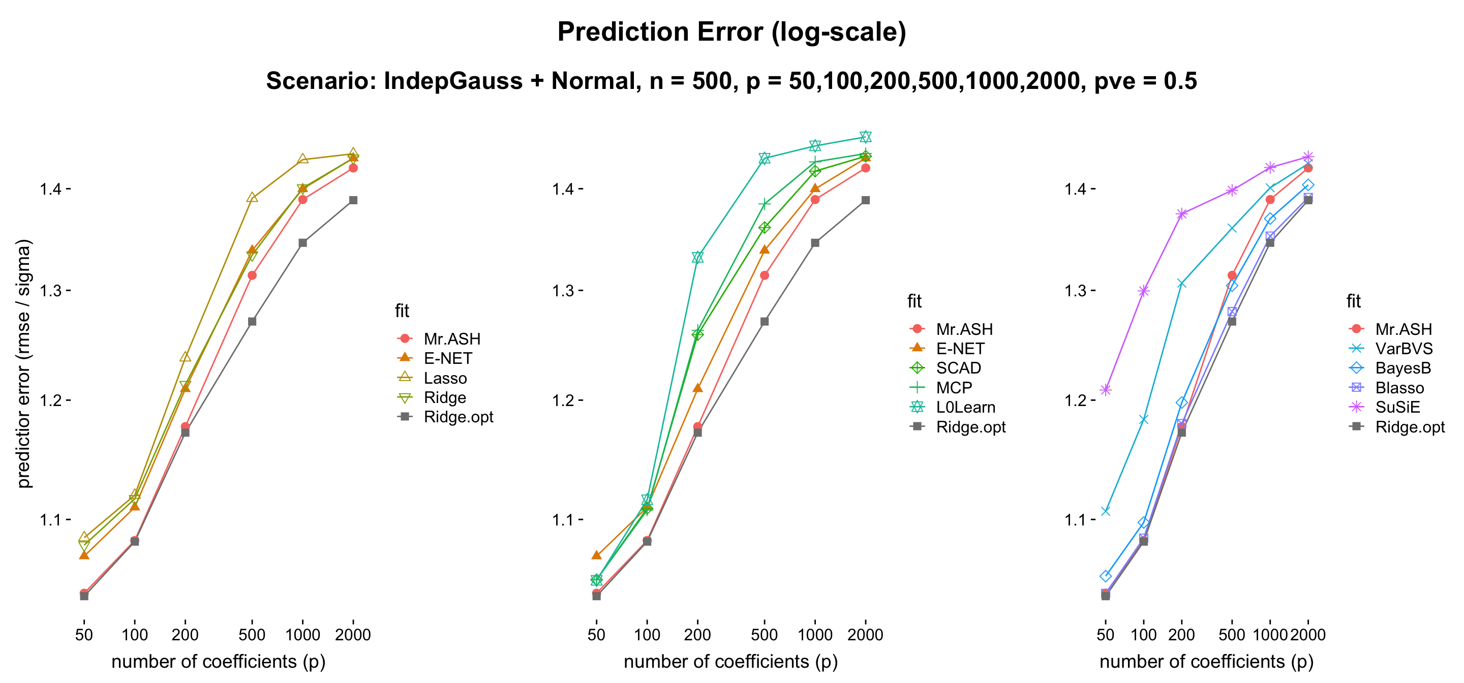
- Discussion: The message here is MR.ASH performs reasonably well, and the only penalized linear regression method that outperforms Ridge with cross-validation. However, let us mention that Blasso (Bayesian Lasso) performs the best, which uses a non-sparse Laplace prior on \(\beta\). Also, BayesB performs better than MR.ASH, which uses a spike-and-slab prior on \(\beta\).
This experiment is to compare the flexibility of convex/non-convex shrinkage operators (E-NET, SCAD, MCP, L0Learn) vs MR.ASH shrinkage operator. The default setting applies to all but the signal shape and PVE = 0.99.
The reason why we set PVE = 0.99, the cross-validated solution of the method (E-NET, SCAD or MCP) acheives a nearly minimum prediction error on the solution path, i.e. the cross-validated solution is nearly the best the method can achieve. Thus we conclude that the cross-validation is fairly accurate. We have checked this by experiment.
- Result:
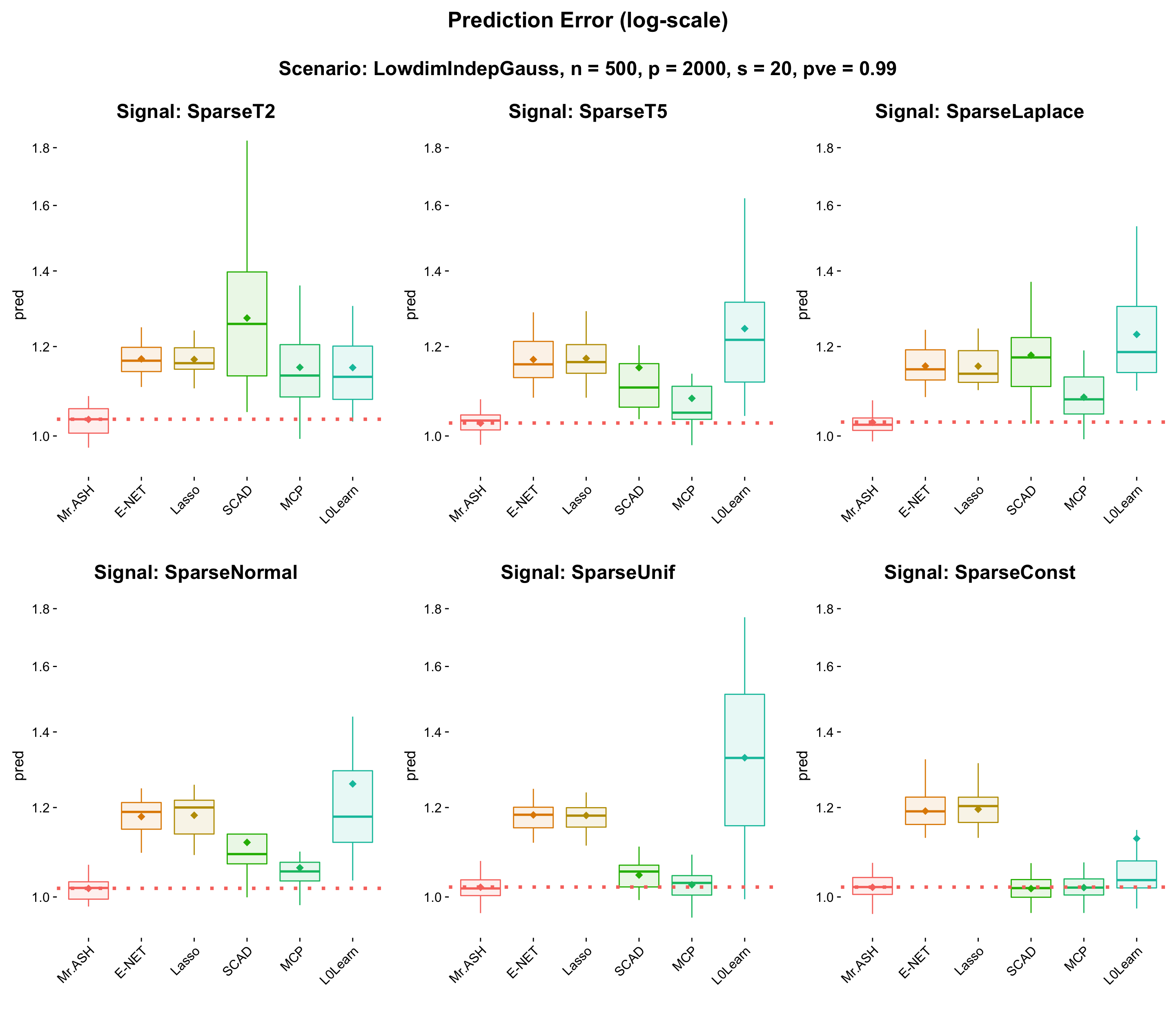
- Discussion: Clearly MR.ASH is an overall winner, outperforming all the other methods. Flexibility of MR.ASH Gaussian mixture prior is illustrated well in the above figure.
Important parameters for high-dimensional regression settings
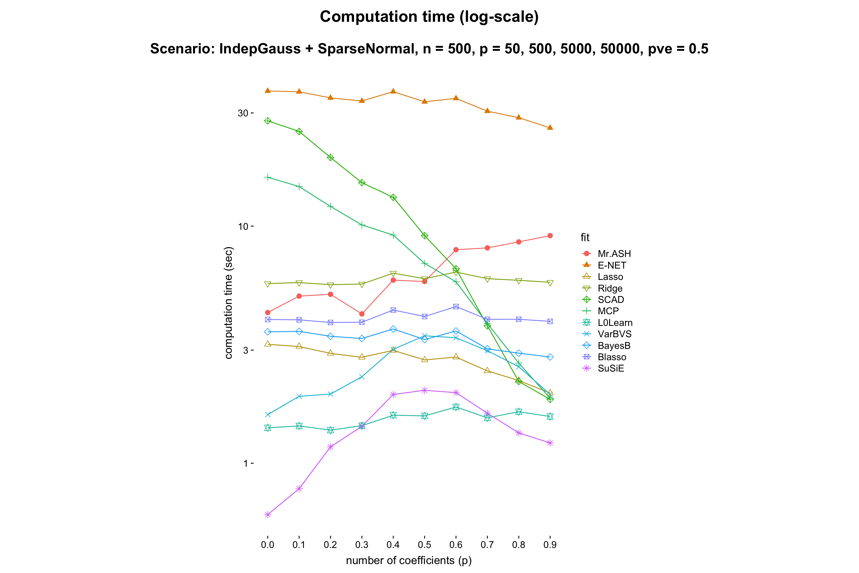
This experiment is to compare performance of the methods when \(p\) varies while the rest being fixed.
- Result:
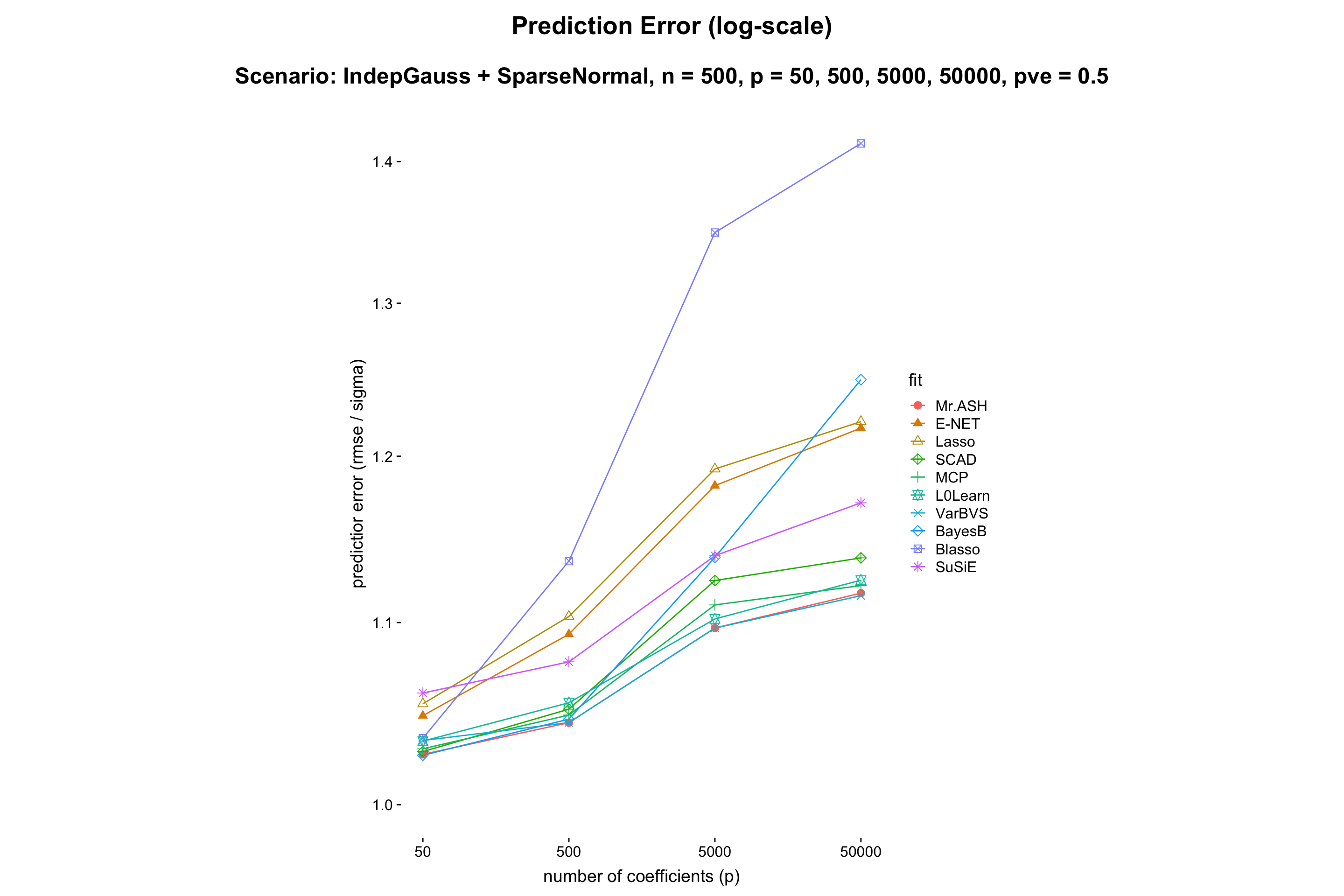
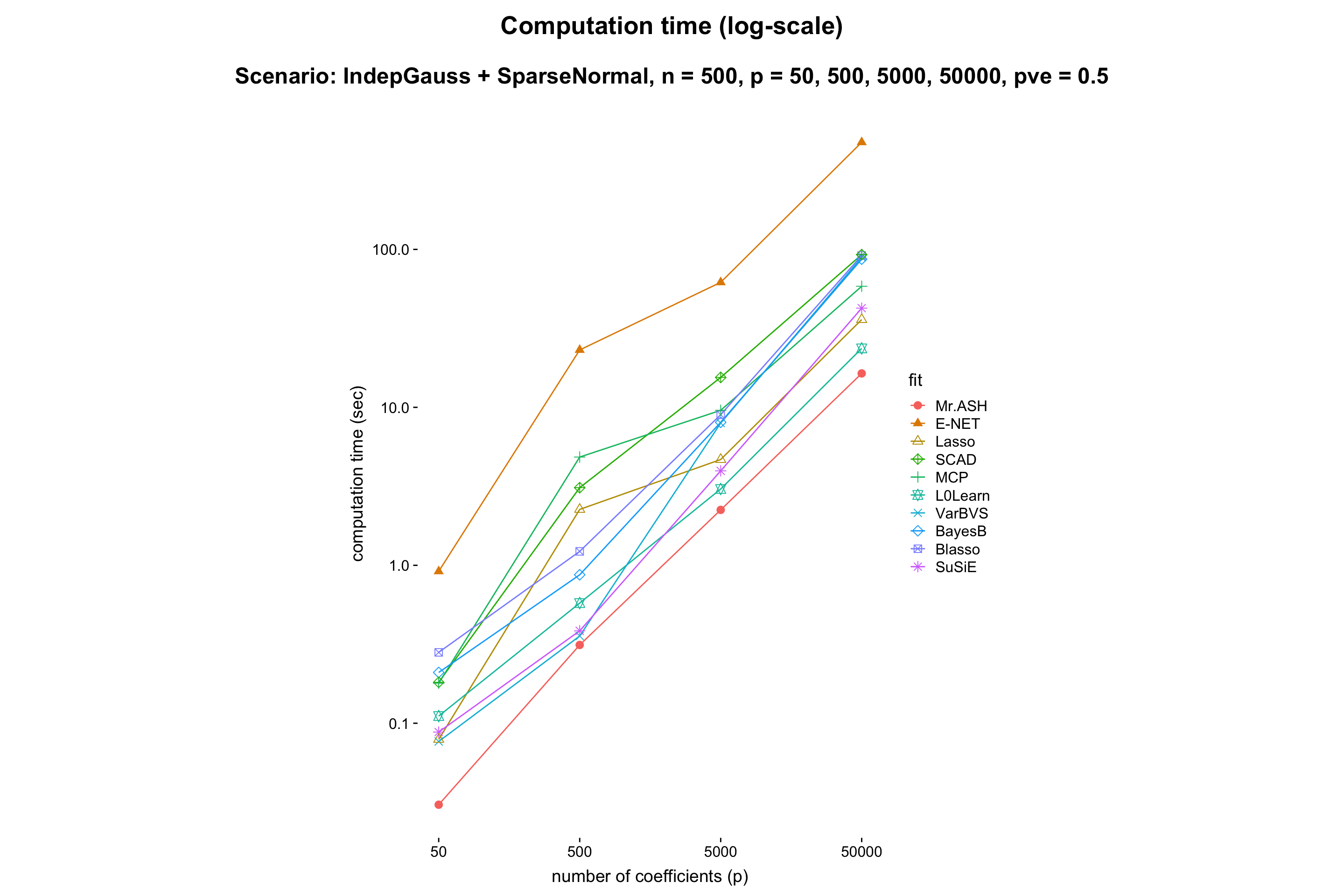
- Discussion: It shows that MR.ASH and VarBVS outperform well. Since the theory says (e.g. Slope meets Lasso: improved oracle bounds and optimality ) that the prediction error scales as \(\sqrt{s\log(p/s)/n}\), and thus we can expect that the prediction error increaese log-linearly in \(p\). One can check this in the above figure.
Also, the computation time of MR.ASH scales linearly in \(\log p\). We conclude that BayesB and Blasso do not scale well for large \(p\).
- Result:
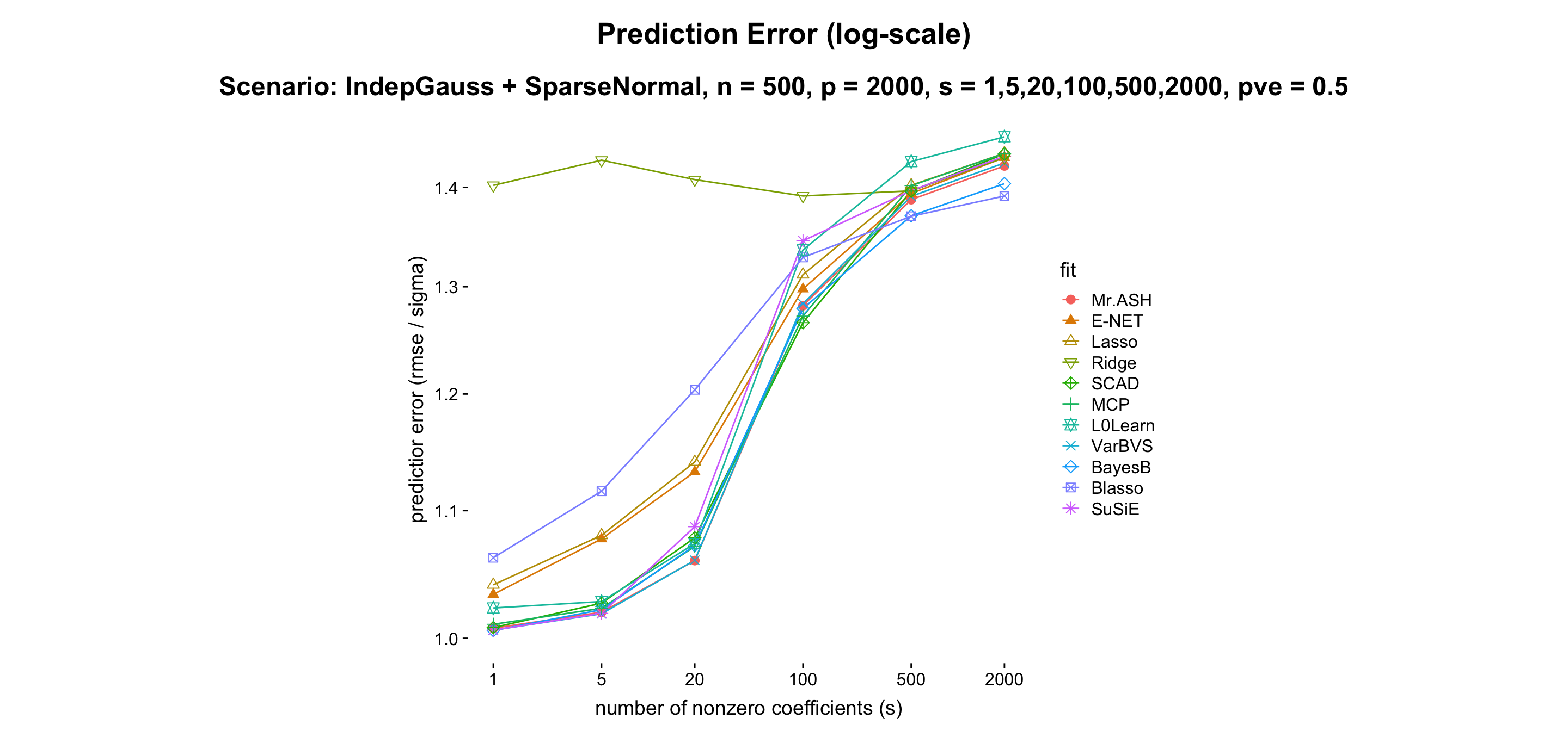
- Discussion: Mr.ASH does well in sparse setting. VARBVS shows very similar performance compared to Mr.ASH. BayesB performs reasonably well for all cases, hence very balanced. Blasso does very well in non-sparse setting.
| Method | Mr.ASH | VARBVS | BayesB | Blasso | Susie | E-NET | Lasso | Ridge | SCAD | MCP | L0Learn |
|---|---|---|---|---|---|---|---|---|---|---|---|
| s = 1 | 1.01 | 1.01 | 1.01 | 1.06 | 1.01 | 1.03 | 1.04 | 1.40 | 1.01 | 1.01 | 1.02 |
| s = 5 | 1.02 | 1.02 | 1.02 | 1.11 | 1.02 | 1.08 | 1.08 | 1.43 | 1.03 | 1.02 | 1.03 |
| s = 20 | 1.06 | 1.06 | 1.07 | 1.20 | 1.09 | 1.13 | 1.14 | 1.41 | 1.08 | 1.07 | 1.07 |
| s = 100 | 1.28 | 1.28 | 1.28 | 1.33 | 1.35 | 1.30 | 1.31 | 1.39 | 1.27 | 1.27 | 1.34 |
| s = 500 | 1.38 | 1.39 | 1.37 | 1.37 | 1.40 | 1.40 | 1.40 | 1.40 | 1.40 | 1.40 | 1.43 |
| s = 2000 | 1.42 | 1.43 | 1.40 | 1.39 | 1.43 | 1.43 | 1.44 | 1.43 | 1.44 | 1.44 | 1.45 |
| Note | sparse | sparse | balanced | non-sparse | sparse | sparse |
- PVE.
- Result:
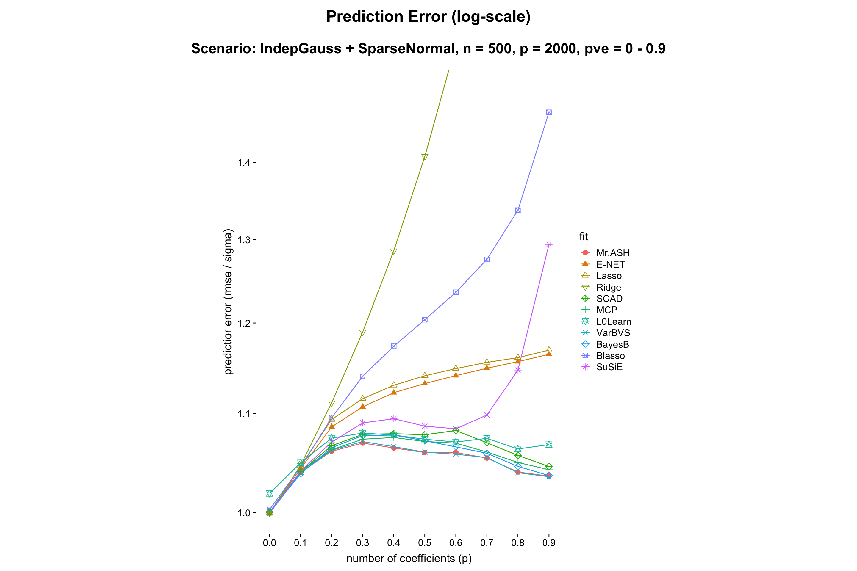
- Discussion: MR.ASH outperforms for all the PVEs. However this experiment setting is favorable for MR.ASH. Thus we can just conclude, for safety, that the relative performance does not depend very much on PVE, but Ridge, SuSiE and Blasso suffer for high PVE.
Performance on different design settings
| Method | Mr.ASH | Mr.ASH.order | MR.ASH.init | VARBVS | BayesB | Blasso | SuSiE | E-NET | Lasso | Ridge | SCAD | MCP | L0Learn |
|---|---|---|---|---|---|---|---|---|---|---|---|---|---|
| LowdimIndepGauss + SuBogdanCandes | 1.012 | 1.012 | 1.012 | 1.012 | 2.315 | 46.19 | 1.012 | 94.60 | 96.82 | 2680 | 1.012 | 1.012 | 1.230 |
| RealGenotype + PointNormal | 1.160 | 1.145 | 1.154 | 1.177 | 1.258 | 1.189 | 1.157 | 1.180 | 1.199 | 1.254 | 1.154 | 1.162 | 1.194 |
| EquiCorrGauss + PointNormal | 1.119 | 1.126 | 1.080 | 1.142 | 1.219 | 1.144 | 1.154 | 1.097 | 1.103 | 1.189 | 1.078 | 1.080 | 1.101 |
| LocalCorrGauss + PointNormal | 1.092 | 1.083 | 1.076 | 1.096 | 1.144 | 1.193 | 1.098 | 1.119 | 1.128 | 1.270 | 1.078 | 1.076 | 1.082 |
| Changepoint + BigSuddenChange | 2.885 | 1.450 | 1.103 | 5.086 | 1.890 | 3.636 | 9.518 | 3.991 | 5.320 | 9.810 | 1.765 | 1.956 | 2.346 |
| Changepoint + OneSmallChange | 2.195 | 1.168 | 1.272 | 1.742 | 8.864 | 4.442 | 1.203 | 3.776 | 4.255 | 6.622 | 1.478 | 2.246 | 3.004 |
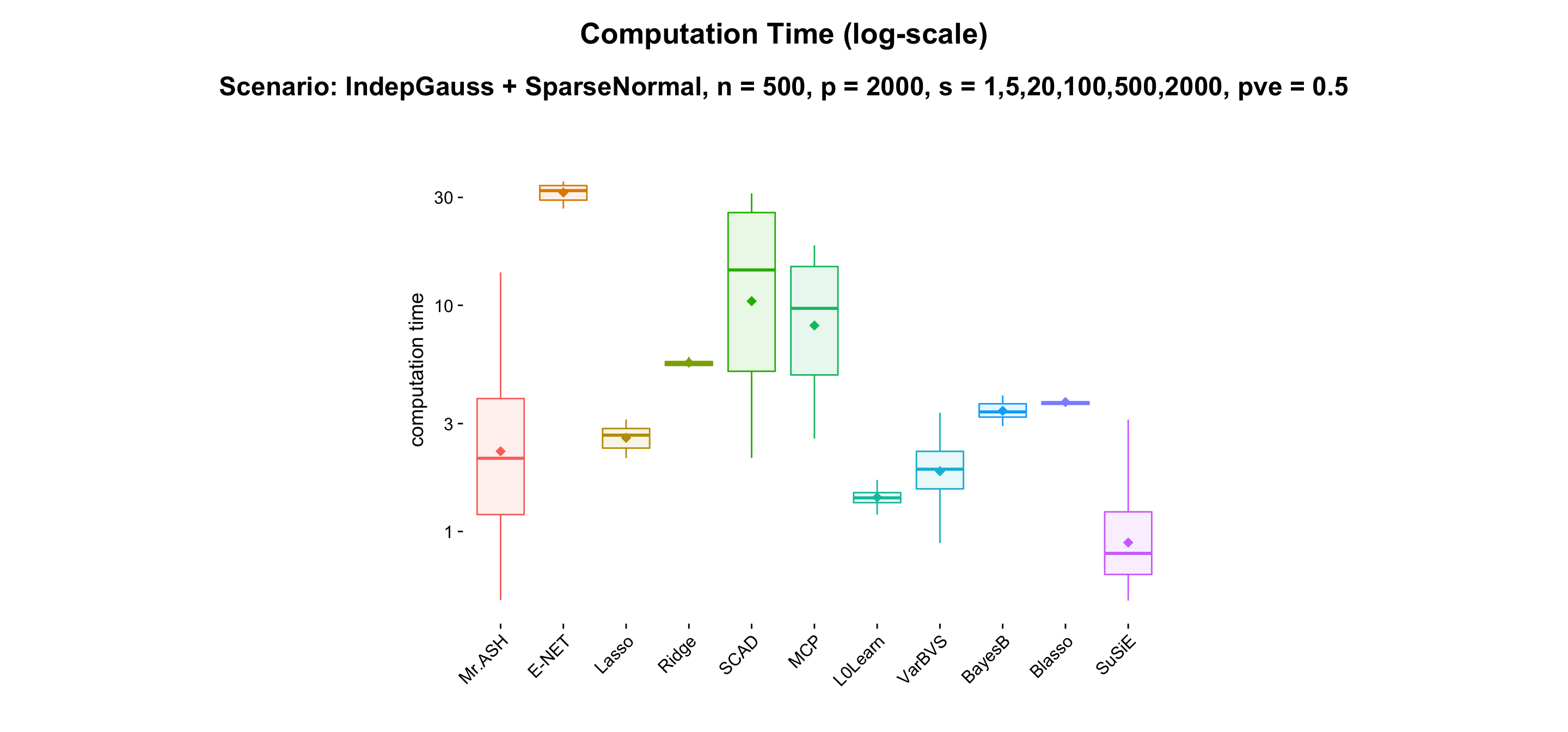
| Computation time | 2.218 | 3.166 | 5.944 | 3.445 | 3.583 | 4.001 | 1.808 | 51.50 | 4.670 | 5.567 | 7.538 | 6.884 | 10.95 |
Results for internal comparison
A list of the update orders we consider is as follows.
random: In each outer loop iteration, we sample a permuation map \(\xi:\{1,\cdots,p\} \to \{1,\cdots,p\}\) uniformly at random and run inner loop iterations with the order based on \(\xi\).increasing: \((1,\cdots,p)\), i.e. in each outer loop iteration, we update \(q_1,q_2,\cdots,q_p\) in this order.lasso.pathorder: we update \(q_j\) prior to \(q_{j'}\) when \(\beta_j\) appears earlier than \(\beta_{j'}\) in the lasso path. If ties occur, thenincreasingorder applies to those ties.scad.pathorder: we update \(q_j\) prior to \(q_{j'}\) when \(\beta_j\) appears earlier than \(\beta_{j'}\) in the scad path. If ties occur, thenincreasingorder applies to those ties.lasso.absorder: we update \(q_j\) prior to \(q_{j'}\) when the lasso solution satisfies \(|\hat\beta_j| \geq |\hat\beta_{j'}|\). If ties occur, thenincreasingorder applies to those ties.univar.absorder: we update \(q_j\) prior to \(q_{j'}\) when the univariate linear regression solution satisfies \(|\hat\beta_j| \geq |\hat\beta_{j'}|\). If ties occur, thenincreasingorder applies to those ties.
A list of the initializations we consider is as follows.
An analysis for the update rule of \(\sigma^2\), based on different parametrizations of the model.
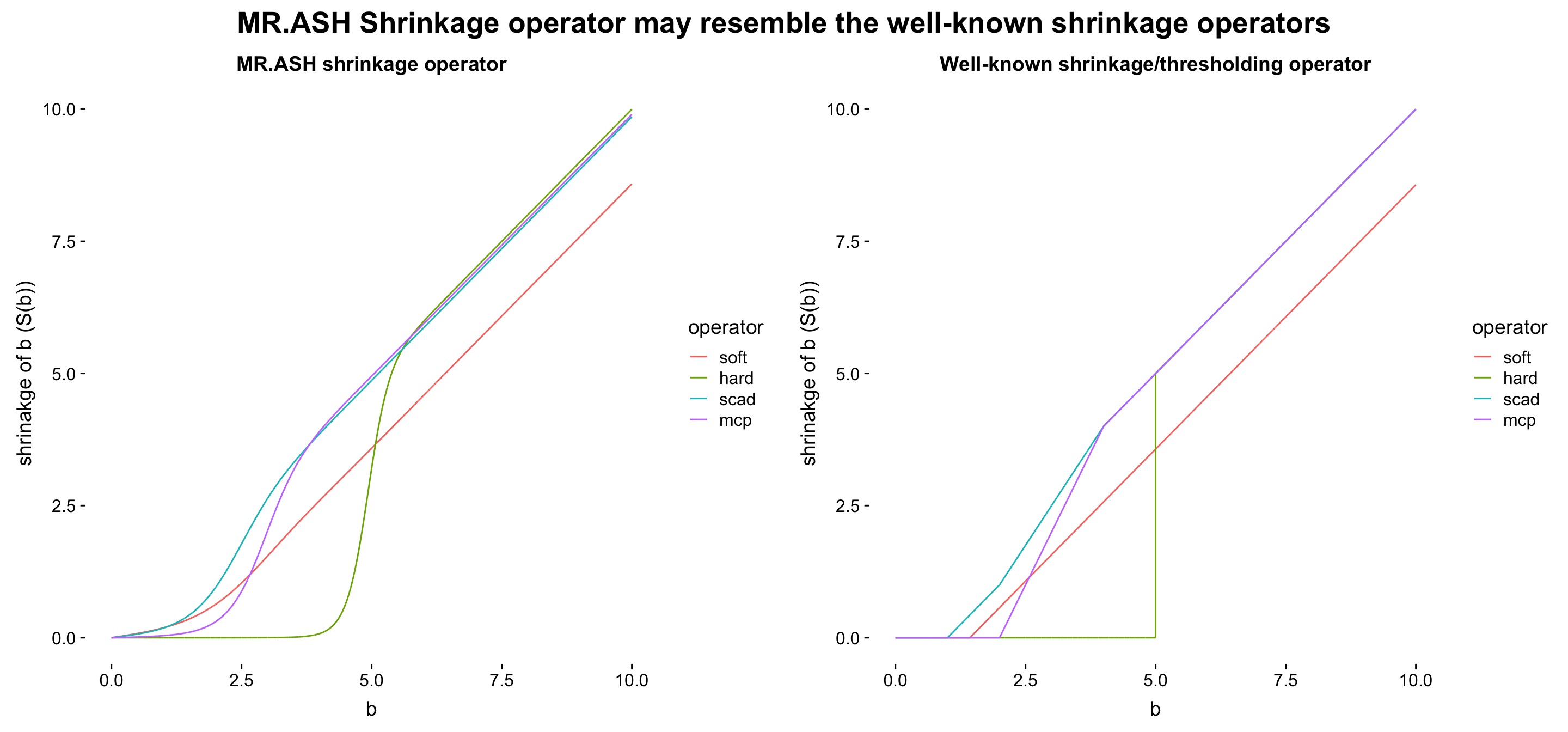
Our story is
the MR.ASH’s shrinkage operator (from a normal mixture prior) is more flexible than other popular shrinkage operators, which is a parametric form of \(\lambda\) (and \(\gamma\) if exists).
VEB can do better than cross validation.
Brief Summary of Comparison Methods
L0Learn
L0Learn R package provides a fast coordinate descent algorithm for the best subset regression.
Fast Best Subset Selection: Coordinate Descent and Local Combinatorial Optimization Algorithms
SCAD, MCP
ncvreg R package provides a fast coordinate descent algorithm for the non-convex penalized linear regression method with well-known penalty functions SCAD and MCP.