Clustering Cusanovich et al (2018) data using topic proportions with K = 13 topics
Kaixuan Luo
Last updated: 2021-02-03
Checks: 7 0
Knit directory: scATACseq-topics/
This reproducible R Markdown analysis was created with workflowr (version 1.6.2). The Checks tab describes the reproducibility checks that were applied when the results were created. The Past versions tab lists the development history.
Great! Since the R Markdown file has been committed to the Git repository, you know the exact version of the code that produced these results.
Great job! The global environment was empty. Objects defined in the global environment can affect the analysis in your R Markdown file in unknown ways. For reproduciblity it's best to always run the code in an empty environment.
The command set.seed(20200729) was run prior to running the code in the R Markdown file. Setting a seed ensures that any results that rely on randomness, e.g. subsampling or permutations, are reproducible.
Great job! Recording the operating system, R version, and package versions is critical for reproducibility.
Nice! There were no cached chunks for this analysis, so you can be confident that you successfully produced the results during this run.
Great job! Using relative paths to the files within your workflowr project makes it easier to run your code on other machines.
Great! You are using Git for version control. Tracking code development and connecting the code version to the results is critical for reproducibility.
The results in this page were generated with repository version 91cab4b. See the Past versions tab to see a history of the changes made to the R Markdown and HTML files.
Note that you need to be careful to ensure that all relevant files for the analysis have been committed to Git prior to generating the results (you can use wflow_publish or wflow_git_commit). workflowr only checks the R Markdown file, but you know if there are other scripts or data files that it depends on. Below is the status of the Git repository when the results were generated:
Ignored files:
    Ignored:    .Rhistory
    Ignored:    .Rproj.user/
    Ignored:    output/plotly/Buenrostro_2018_Chen2019pipeline/

Untracked files:
    Untracked:  analysis/gene_analysis_Buenrostro2018_Chen2019pipeline.Rmd
    Untracked:  analysis/process_data_Buenrostro2018_Chen2019.Rmd
    Untracked:  output/clustering-Cusanovich2018.rds
    Untracked:  scripts/fit_all_models_Buenrostro_2018_chromVar_scPeaks_filtered.sbatch
    Untracked:  scripts/fit_models_Cusanovich2018_tissues.sh

Unstaged changes:
    Modified:   analysis/assess_fits_Cusanovich2018.Rmd
    Modified:   analysis/gene_analysis_Cusanovich2018.Rmd
    Modified:   analysis/index.Rmd
    Modified:   analysis/motif_analysis_Buenrostro2018_Chen2019pipeline.Rmd
    Modified:   analysis/plots_Cusanovich2018.Rmd
    Modified:   analysis/process_data_Cusanovich2018.Rmd
    Modified:   scripts/fit_poisson_nmf.sbatch
    Modified:   scripts/prefit_poisson_nmf.sbatch
Note that any generated files, e.g. HTML, png, CSS, etc., are not included in this status report because it is ok for generated content to have uncommitted changes.
These are the previous versions of the repository in which changes were made to the R Markdown (analysis/clusters_Cusanovich2018_k13.Rmd) and HTML (docs/clusters_Cusanovich2018_k13.html) files. If you've configured a remote Git repository (see ?wflow_git_remote), click on the hyperlinks in the table below to view the files as they were in that past version.
| File | Version | Author | Date | Message |
|---|---|---|---|---|
| Rmd | 91cab4b | kevinlkx | 2021-02-03 | added k-means results on PCA of topic proportions, and merged two clusters, and moved PCA plots to the end |
| html | f8ec9d7 | kevinlkx | 2020-12-02 | Build site. |
| Rmd | b30b5c6 | kevinlkx | 2020-12-02 | print outlier cells in c15 |
| html | 24c6d8b | kevinlkx | 2020-12-02 | Build site. |
| Rmd | 586af90 | kevinlkx | 2020-12-02 | wflow_publish("analysis/clusters_Cusanovich2018_k13.Rmd") |
| html | 019f436 | kevinlkx | 2020-12-02 | Build site. |
| Rmd | 06efc2b | kevinlkx | 2020-12-02 | zoom into a few clusters |
| html | 96392bf | kevinlkx | 2020-12-02 | Build site. |
| Rmd | 8db261b | kevinlkx | 2020-12-02 | wflow_publish("analysis/clusters_Cusanovich2018_k13.Rmd") |
| html | deead06 | kevinlkx | 2020-12-01 | Build site. |
| Rmd | 2af43a8 | kevinlkx | 2020-12-01 | update tissue colors |
| html | 06b9bc9 | kevinlkx | 2020-12-01 | Build site. |
| Rmd | bc7e770 | kevinlkx | 2020-12-01 | update tissue colors |
| html | 6c97fa9 | kevinlkx | 2020-12-01 | Build site. |
| Rmd | ab321de | kevinlkx | 2020-12-01 | refine kmeans clusters and add cell label distributions |
| html | e57dfd4 | kevinlkx | 2020-10-21 | Build site. |
| Rmd | a88649d | kevinlkx | 2020-10-21 | wflow_publish("analysis/clusters_Cusanovich2018_k13.Rmd") |
| Rmd | 137c252 | kevinlkx | 2020-10-21 | set toc = yes |
| html | 4c0ab95 | kevinlkx | 2020-10-21 | Build site. |
| html | 9d31a9f | kevinlkx | 2020-10-21 | Build site. |
| Rmd | c00f12b | kevinlkx | 2020-10-21 | update colors and interpret clusters with tissue labels |
| html | 32ed5ae | kevinlkx | 2020-10-21 | Build site. |
| Rmd | 82292d5 | kevinlkx | 2020-10-21 | update colors and interpret clusters with tissue labels |
| html | b8a48b9 | kevinlkx | 2020-10-20 | Build site. |
| Rmd | a4daf6d | kevinlkx | 2020-10-20 | clustering with k = 13 topics |
| html | ac8ca65 | kevinlkx | 2020-10-20 | Build site. |
| Rmd | 98920ed | kevinlkx | 2020-10-20 | clustering with k = 13 topics |
| html | a38788b | kevinlkx | 2020-10-20 | Build site. |
| Rmd | f8bea96 | kevinlkx | 2020-10-20 | clustering with k = 13 topics |
Here we explore the structure in the Cusanovich et al (2018) ATAC-seq data inferred from the multinomial topic model with \(k = 13\).
Load packages and some functions used in this analysis.
library(Matrix)
library(dplyr)
library(ggplot2)
library(cowplot)
library(fastTopics)
source("code/plots.R")
Load the data. The counts are no longer needed at this stage of the analysis.
data.dir <- "/project2/mstephens/kevinluo/scATACseq-topics/data/Cusanovich_2018/processed_data/"
load(file.path(data.dir, "Cusanovich_2018.RData"))
rm(counts)
Load the model fit
fit.dir <- "/project2/mstephens/kevinluo/scATACseq-topics/output/Cusanovich_2018"
fit <- readRDS(file.path(fit.dir, "/fit-Cusanovich2018-scd-ex-k=13.rds"))$fit
fit_multinom <- poisson2multinom(fit)
About the samples: The study measured single cell chromatin accessibility for 17 samples spanning 13 different tissues in 8-week old mice.
cat(nrow(samples), "samples (cells). \n")
# 81173 samples (cells).
Tissues:
samples$tissue <- as.factor(samples$tissue)
cat(length(levels(samples$tissue)), "tissues. \n")
# table(samples$tissue)

colors_tissues <- c("darkblue",    # BoneMarrow
                    "gray30",      # Cerebellum
                    "red",         # Heart
                    "springgreen", # Kidney
                    "brown",       # LargeIntestine
                    "purple",      # Liver
                    "deepskyblue", # Lung
                    "black",       # PreFrontalCortex
                    "darkgreen",   # SmallIntestine
                    "plum",        # Spleen
                    "gold",        # Testes
                    "darkorange",  # Thymus
                    "gray")        # WholeBrain
# 13 tissues.
Cell types labels:
samples$cell_label <- as.factor(samples$cell_label)
cat(length(levels(samples$cell_label)), "cell types \n")
# table(samples$cell_label)
# 40 cell types
Structure plots
The structure plots below summarize the topic proportions in the samples grouped by different tissues.
Visualize by Structure plot grouped by tissues
set.seed(10)
colors_topics <- c("#a6cee3","#1f78b4","#b2df8a","#33a02c","#fb9a99","#e31a1c",
                   "#fdbf6f","#ff7f00","#cab2d6","#6a3d9a","#ffff99","#b15928",
                   "gray")
samples$tissue <- as.factor(samples$tissue)

rows <- sample(nrow(fit$L),4000)

p.structure.1 <- structure_plot(select(fit_multinom,loadings = rows),
                     grouping = samples[rows, "tissue"],n = Inf,gap = 40,
                     perplexity = 50,topics = 1:13,colors = colors_topics,
                     num_threads = 4,verbose = FALSE)

print(p.structure.1)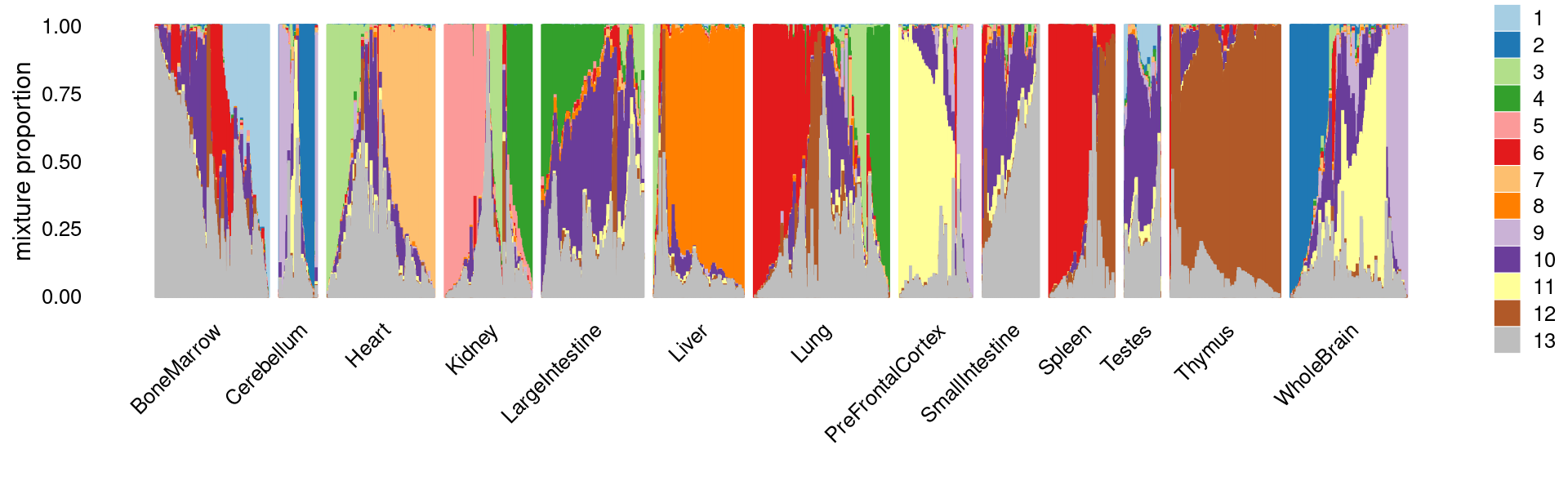
Perform k-means clustering on topic proportions
Define clusters using k-means, and then create structure plot based on the clusters from k-means.
k-means clustering (using 15 clusters) on topic proportions
set.seed(10)
clusters <- factor(kmeans(fit_multinom$L,centers = 15,iter.max = 100)$cluster)
summary(clusters)

rows <- sample(nrow(fit$L),4000)

p.structure.kmeans <- structure_plot(select(fit_multinom,loadings = rows),
                                        grouping = clusters[rows],n = Inf,gap = 20,
                                        perplexity = 50,topics = 1:13,colors = colors_topics,
                                        num_threads = 4,verbose = FALSE)
print(p.structure.kmeans)
#     1     2     3     4     5     6     7     8     9    10    11    12    13
#  2740  3868  3775  3879  3645  3651 12037  2955  6045 12026  6068  3582  9319
#    14    15
#  3411  4172
First do PCA on topic proportions and then do k-means clustering (using 15 clusters). Results are the same as the results from running k-means directly on the topic proportions.
set.seed(10)
pca <- prcomp(fit_multinom$L)$x
clusters2 <- factor(kmeans(pca,centers = 15,iter.max = 100)$cluster)
summary(clusters2)

rows <- sample(nrow(fit$L),4000)

p.structure.kmeans <- structure_plot(select(fit_multinom,loadings = rows),
                                        grouping = clusters2[rows],n = Inf,gap = 20,
                                        perplexity = 50,topics = 1:13,colors = colors_topics,
                                        num_threads = 4,verbose = FALSE)
print(p.structure.kmeans)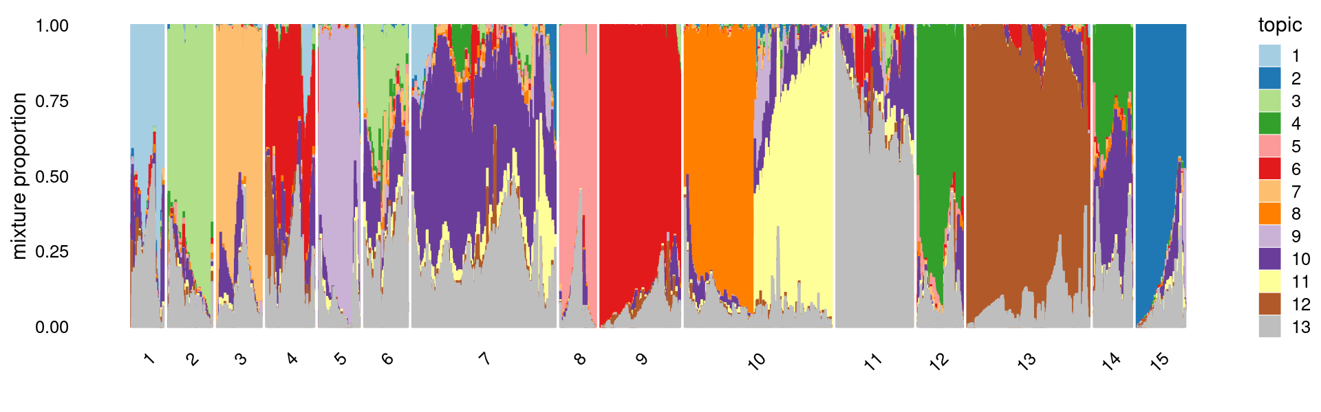
length(which(clusters != clusters2))
#     1     2     3     4     5     6     7     8     9    10    11    12    13
#  2740  3868  3775  3879  3645  3651 12037  2955  6045 12026  6068  3582  9319
#    14    15
#  3411  4172
# [1] 0
Refine k-means clusters: - Split cluster 10 into two clusters. - merge cluster 4 and 9
Structure plot based on refined clusters
set.seed(10)
clusters.refined <- as.numeric(clusters)
clusters.refined[which(clusters == 9)] <- 4

# clusters.refined[which(clusters == 10 & fit_multinom$L[,8] >= 0.2)] <- 16
# clusters.refined[which(clusters == 10 & fit_multinom$L[,8] < 0.2)] <- 17

clusters.refined[which(clusters == 10)] <- kmeans(fit_multinom$L[which(clusters == 10), ],centers = 2)$cluster+15
clusters.refined <- factor(clusters.refined, labels = paste0("c", c(1:length(unique(clusters.refined)))))

samples$cluster_kmeans <- clusters.refined

rows <- sample(nrow(fit$L),4000)

p.structure.kmeans.refined <- structure_plot(select(fit_multinom,loadings = rows),
                                             grouping = clusters.refined[rows],n = Inf,gap = 40,
                                             perplexity = 50,topics = 1:13,colors = colors_topics,
                                             num_threads = 4,verbose = FALSE)
print(p.structure.kmeans.refined)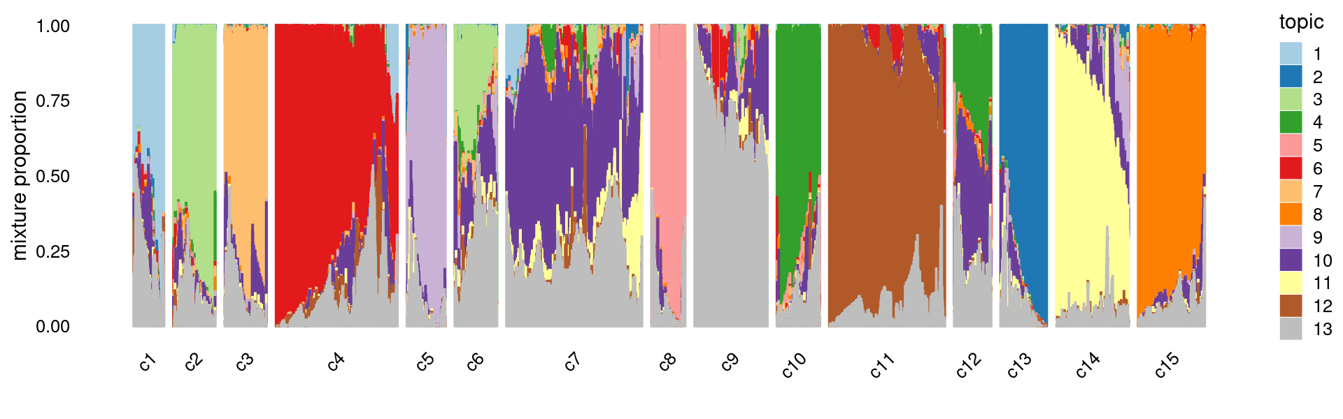
Save the clustering results to an RDS file
out.dir <- "/project2/mstephens/kevinluo/scATACseq-topics/output/Cusanovich_2018"
saveRDS(samples, paste0(out.dir, "/samples-clustering-Cusanovich2018.rds"))

samples <- readRDS("output/samples-clustering-Cusanovich2018.rds")
clusters.refined <- samples$cluster_kmeans
print(table(samples$cluster_kmeans))
Plot the distribution of tissues in each cluster
Tissue composition in each cluster:
library(plyr);library(dplyr)
# ------------------------------------------------------------------------------
# You have loaded plyr after dplyr - this is likely to cause problems.
# If you need functions from both plyr and dplyr, please load plyr first, then dplyr:
# library(plyr); library(dplyr)
# ------------------------------------------------------------------------------
#
# Attaching package: 'plyr'
# The following objects are masked from 'package:dplyr':
#
#     arrange, count, desc, failwith, id, mutate, rename, summarise,
#     summarize
library(RColorBrewer)

freq_cluster_tissue <- count(samples, vars=c("cluster_kmeans","tissue"))

# stacked barplot for the counts of tissues by clusters
p.barplot <- ggplot(freq_cluster_tissue, aes(fill=tissue, y=freq, x=cluster_kmeans)) +
  geom_bar(position="fill", stat="identity") +
  theme_classic() + xlab("Cluster") + ylab("Proportion of cells") +
  scale_fill_manual(values = colors_tissues) +
  guides(fill=guide_legend(ncol=2)) +
  theme(
  legend.title = element_text(size = 10),
  legend.text = element_text(size = 8)
  )
print(p.barplot)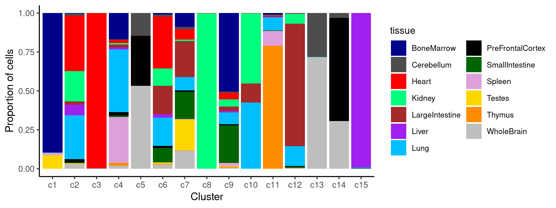
We can see a few clusters are tissue specific:
- cluster c3 is heart specific;
- cluster c8 is kidney specific;
- cluster c15 is liver specific;
- cluster c1 is primarily bone marrow;
- cluster c11 is primarily thymus.
Some clusters are combinations of related tissues:
- cluster c4 is half lung and half spleen;
- cluster c5 and c14 are mainly from pre-frontal cortex, whole brain (and cerebellum) -- all neuron related.
- cluster c14 is also from whole brain and cerebellum.
- cluster c10 is mainly from Kidney, LargeIntestine, and Lung.
Some clusters are more heterogeneous mixtures of different tissues.
Distribution of tissue labels by cluster.
freq_table_cluster_tissue <- with(samples,table(tissue,cluster_kmeans))
print(freq_table_cluster_tissue)
#                   cluster_kmeans
# tissue               c1   c2   c3   c4   c5   c6   c7   c8   c9  c10  c11  c12
#   BoneMarrow       2455   15    0 1675    0   33 1060    0 3063    0  102    0
#   Cerebellum          0   51    0   37  525   44  191    0   42    0    0   15
#   Heart               0 1374 3768  194    3 1225  803    5  259    3   13    3
#   Kidney              0  757    0   95    0  402   98 2950  280 1614   19  215
#   LargeIntestine      0   73    1  178    4  665 2778    0  172  441   94 2680
#   Liver               0  268    0  136    0   84   31    0   50    1   34    4
#   Lung                2 1093    5 4002    2  659 1010    0  465 1521  773  434
#   PreFrontalCortex    0   75    0  215 1169   48  118    0   49    0    1   19
#   SmallIntestine      0   22    0   84    0  341 2112    0 1457    1   27   18
#   Spleen             43    3    0 2937    0    5   24    0  116    0  892    0
#   Testes            240   19    0    3    0   37 2379    0   38    0    0    4
#   Thymus              0    2    1  172    0    9   32    0   30    1 7363    7
#   WholeBrain          0  116    0  196 1942   99 1401    0   47    0    1   12
#                   cluster_kmeans
# tissue              c13  c14  c15
#   BoneMarrow          0    0    0
#   Cerebellum       1177  196    0
#   Heart               0    0    0
#   Kidney              0    0    1
#   LargeIntestine      0    0    0
#   Liver               1    0 5558
#   Lung                2    2   26
#   PreFrontalCortex    4 4261    0
#   SmallIntestine      0    0   15
#   Spleen              0    0    0
#   Testes              0    0    3
#   Thymus              0    0    0
#   WholeBrain       2988 1964    0
Distribution of cell labels by cluster.
freq_table_cluster_celllabel <- with(samples,table(cell_label,cluster_kmeans))
print(freq_table_cluster_celllabel)
#                             cluster_kmeans
# cell_label                     c1   c2   c3   c4   c5   c6   c7   c8   c9  c10
#   Activated B cells             0    0    0  477    0    0    0    0   23    0
#   Alveolar macrophages          0    0    0  507    0    2   16    0   34    0
#   Astrocytes                    0    0    0    0 1574   11   58    0   20    0
#   B cells                       0    0    0 5086    0    3  648    0   34    0
#   Cardiomyocytes                0   15 3773    1    0   42  169    0   76    0
#   Cerebellar granule cells      0    0    0    9    0    3  306    0   19    0
#   Collecting duct               0    0    0    0    0   10    0    0    5  124
#   Collisions                    6    2    0  340  423   15  166    0   64    0
#   DCT/CD                        0    0    0    0    0    1    0    1    6  441
#   Dendritic cells               1    0    0  840    0    2   12    0  102    0
#   Distal convoluted tubule      0    0    0    0    0    0    0    0    6  301
#   Endothelial I (glomerular)    0  386    0    0    0  158    0    0    8    0
#   Endothelial I cells           0  512    0    0    0  438    1    0    1    0
#   Endothelial II cells          0 2405    0   15    0  574    7    0   15    0
#   Enterocytes                   0    0    0    0    1   11 1585    0   54  442
#   Erythroblasts              2420    0    0   37    0    0   79    0  275    0
#   Ex. neurons CPN               0    0    0    0    0    0   10    0    0    0
#   Ex. neurons CThPN             0    0    0    0    0    0   91    0    0    0
#   Ex. neurons SCPN              0    0    0    0    0    0   40    0   32    0
#   Hematopoietic progenitors     0    0    0   26    0    1  899    0 2499    0
#   Hepatocytes                   0    0    0    2    0    5   11    0   44    0
#   Immature B cells              0    0    0  353    0    0    0    0  218    0
#   Inhibitory neurons            0    0    0    3   68   27  754    0    8    0
#   Loop of henle                 0    1    0    0    0    8    2    1   11  718
#   Macrophages                   0    0    0  464    0   14  191    0   42    0
#   Microglia                     0    1    0  385    1    3   31    0    1    0
#   Monocytes                    69    0    0 1019    0    1   50    0   32    0
#   NK cells                      0    0    0  231    0    1    2    0   16    0
#   Oligodendrocytes              0    0    0    1 1506    1   30    0   17    0
#   Podocytes                     0  369    0    0    0  113    0    0   16    0
#   Proximal tubule               0    1    0    1    0   16   33 2361  132    7
#   Proximal tubule S3            0    0    0    0    0    0    2  592    0    0
#   Purkinje cells                0    0    0    0    1    2   50    0    0    0
#   Regulatory T cells            3    0    0   17    0    1    7    0    4    0
#   SOM+ Interneurons             0    0    0    0    7    8   66    0    5    0
#   Sperm                       240    0    0    0    0    1 1814    0   32    0
#   T cells                       1    1    0   35    1    7  104    0   50    0
#   Type I pneumocytes            0    0    0    1    0    3    0    0   27 1415
#   Type II pneumocytes           0    8    0    0    0   14    0    0    1   66
#   Unknown                       0  167    2   74   63 2155 4803    0 2139   68
#                             cluster_kmeans
# cell_label                    c11  c12  c13  c14  c15
#   Activated B cells             0    0    0    0    0
#   Alveolar macrophages          0    0    0    0    0
#   Astrocytes                    0    0    0    3    0
#   B cells                       0    1    0    0    0
#   Cardiomyocytes                0    0    0    0    0
#   Cerebellar granule cells      0    0 3762    0    0
#   Collecting duct               0   25    0    0    0
#   Collisions                   11    8   97   86    0
#   DCT/CD                        0   57    0    0    0
#   Dendritic cells               0    1    0    0    0
#   Distal convoluted tubule      0   12    0    0    0
#   Endothelial I (glomerular)    0    0    0    0    0
#   Endothelial I cells           0    0    0    0    0
#   Endothelial II cells          1    1    1    0    0
#   Enterocytes                   0 2690    0    0    0
#   Erythroblasts                 0    0    0    0    0
#   Ex. neurons CPN               0    0    0 1822    0
#   Ex. neurons CThPN             0    0    0 1449    0
#   Ex. neurons SCPN              0    0    0 1394    0
#   Hematopoietic progenitors     0    0    0    0    0
#   Hepatocytes                   0    0    0    0 5602
#   Immature B cells              0    0    0    0    0
#   Inhibitory neurons            0    0    3  965    0
#   Loop of henle                 0   74    0    0    0
#   Macrophages                   0    0    0    0    0
#   Microglia                     0    0    0    0    0
#   Monocytes                     2    0    0    0    0
#   NK cells                     71    0    0    0    0
#   Oligodendrocytes              0    0    0    3    0
#   Podocytes                     0    0    0    0    0
#   Proximal tubule               0   19    0    0    0
#   Proximal tubule S3            0    0    0    0    0
#   Purkinje cells                0    0  262    5    0
#   Regulatory T cells          475    0    0    0    0
#   SOM+ Interneurons             0    0    1  466    0
#   Sperm                         0    2    0    0    0
#   T cells                    8753    2    0    0    0
#   Type I pneumocytes            6  170    0    0    0
#   Type II pneumocytes           0   68    0    0    0
#   Unknown                       0  281   46  230    1
zoom into a few clusters:
Structure plot for c2 cluster: Group samples by tissue labels first, then by cell labels
rows.c2 <- which(samples$cluster_kmeans == "c2")

tissue_labels_cluster <- as.factor(as.character(samples[rows.c2, "tissue"]))
cell_labels_cluster <- as.factor(as.character(samples[rows.c2, "cell_label"]))

sort(table(tissue_labels_cluster), decreasing = T)
sort(table(cell_labels_cluster), decreasing = T)

p.structure <- structure_plot(select(fit_multinom,loadings = rows.c2),
                     grouping = tissue_labels_cluster,
                     rows = order(cell_labels_cluster),
                     n = Inf,gap = 40,
                     perplexity = 50,topics = 1:13,colors = colors_topics,
                     num_threads = 4,verbose = FALSE)
print(p.structure)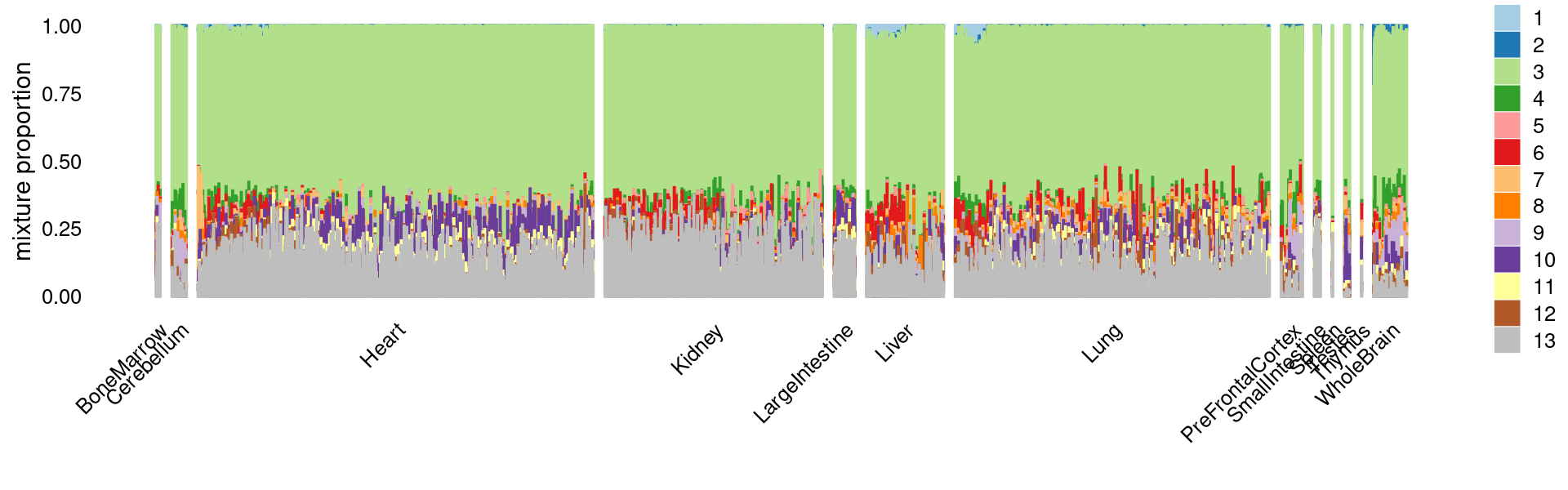
# tissue_labels_cluster
#            Heart             Lung           Kidney            Liver
#             1374             1093              757              268
#       WholeBrain PreFrontalCortex   LargeIntestine       Cerebellum
#              116               75               73               51
#   SmallIntestine           Testes       BoneMarrow           Spleen
#               22               19               15                3
#           Thymus
#                2
# cell_labels_cluster
#       Endothelial II cells        Endothelial I cells
#                       2405                        512
# Endothelial I (glomerular)                  Podocytes
#                        386                        369
#                    Unknown             Cardiomyocytes
#                        167                         15
#        Type II pneumocytes                 Collisions
#                          8                          2
#              Loop of henle                  Microglia
#                          1                          1
#            Proximal tubule                    T cells
#                          1                          1
breaks <- c(0,1,5,10,100,Inf)
fit.c2 <- select(fit_multinom,loadings = rows.c2)
p.pca.c2 <- pca_plot(fit.c2,fill = "none")
p.pca.hexbin.c2 <- pca_hexbin_plot(fit.c2,breaks = breaks) + guides(fill = "none")
plot_grid(p.pca.c2, p.pca.hexbin.c2)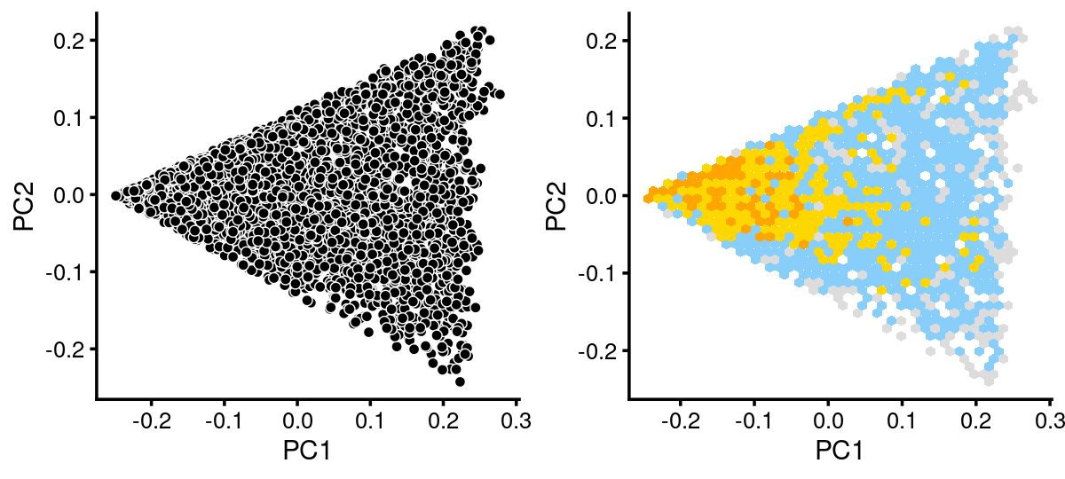
The variation in PCs 1 and 2 is mostly produced by topics 3,13
p.pca.c2.topics <- pca_plot(fit.c2,k = c(3,13))
print(p.pca.c2.topics)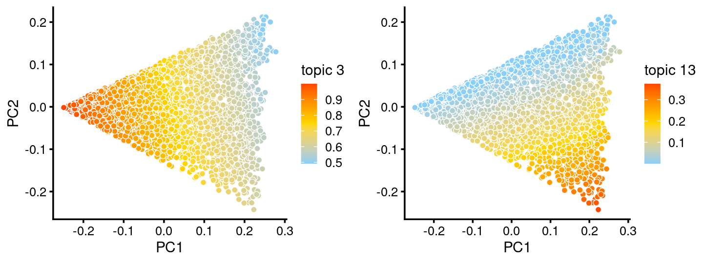
colors_celllabels_c2 <- c("firebrick","dodgerblue","forestgreen",
                           "darkmagenta","darkorange","gold","darkblue",
                           "peru","greenyellow","olivedrab",
                           "darkgray", "black")

p.pca.c2.tissue <- labeled_pca_plot(fit.c2,1:2,samples[rows.c2, "tissue"],font_size = 7,
                       colors = colors_tissues, legend_label = "tissue")
p.pca.c2.cell <- labeled_pca_plot(fit.c2,1:2,samples[rows.c2, "cell_label"],font_size = 7,
                        colors = colors_celllabels_c2, legend_label = "cell_label")
plot_grid(p.pca.c2.tissue,p.pca.c2.cell,rel_widths = c(8,9))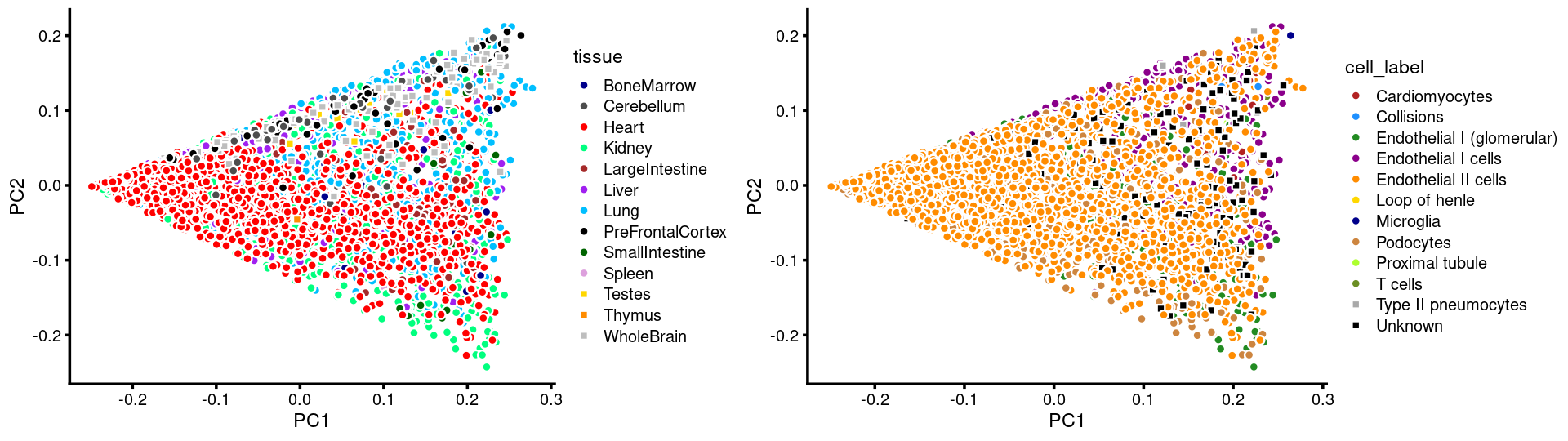
| Version | Author | Date |
|---|---|---|
| 96392bf | kevinlkx | 2020-12-02 |
zoom into cluster c14
Structure plot of c14 cluster: Group samples by tissue labels first, then by cell labels
rows.c14 <- which(samples$cluster_kmeans == "c14")

tissue_labels_cluster <- as.factor(as.character(samples[rows.c14, "tissue"]))
cell_labels_cluster <- as.factor(as.character(samples[rows.c14, "cell_label"]))

sort(table(tissue_labels_cluster), decreasing = T)
sort(table(cell_labels_cluster), decreasing = T)

p.structure <- structure_plot(select(fit_multinom,loadings = rows.c14),
                     grouping = tissue_labels_cluster,
                     rows = order(cell_labels_cluster),
                     n = Inf,gap = 40,
                     perplexity = 50,topics = 1:13,colors = colors_topics,
                     num_threads = 4,verbose = FALSE)
print(p.structure)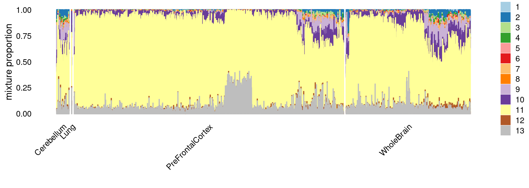
# tissue_labels_cluster
# PreFrontalCortex       WholeBrain       Cerebellum             Lung
#             4261             1964              196                2
# cell_labels_cluster
#    Ex. neurons CPN  Ex. neurons CThPN   Ex. neurons SCPN Inhibitory neurons
#               1822               1449               1394                965
#  SOM+ Interneurons            Unknown         Collisions     Purkinje cells
#                466                230                 86                  5
#         Astrocytes   Oligodendrocytes
#                  3                  3
breaks <- c(0,1,5,10,100,Inf)
fit.c14 <- select(fit_multinom,loadings = rows.c14)
p.pca.c14 <- pca_plot(fit.c14,fill = "none")
p.pca.hexbin.c14 <- pca_hexbin_plot(fit.c14,breaks = breaks) + guides(fill = "none")
plot_grid(p.pca.c14, p.pca.hexbin.c14)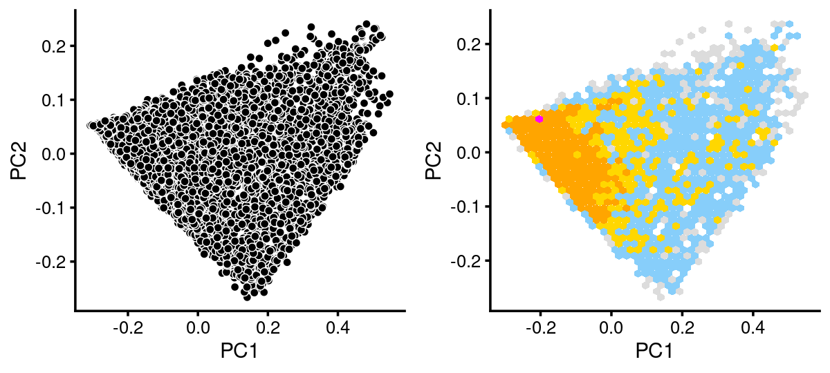
The variation in PCs 1 and 2 is mostly produced by topics 9,10,11
p.pca.c14.topics <- pca_plot(fit.c14,k = c(9,10,11))
print(p.pca.c14.topics)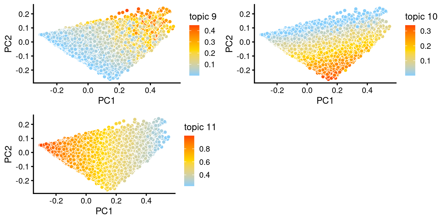
colors_celllabels_c14 <- c("firebrick","dodgerblue","forestgreen",
                           "darkmagenta","darkorange","gold","darkblue",
                           "peru","greenyellow","black")

p.pca.c14.tissue <- labeled_pca_plot(fit.c14,1:2,samples[rows.c14, "tissue"],font_size = 7,
                       colors = colors_tissues, legend_label = "tissue")
p.pca.c14.cell <- labeled_pca_plot(fit.c14,1:2,samples[rows.c14, "cell_label"],font_size = 7,
                        colors = colors_celllabels_c14, legend_label = "cell_label")
plot_grid(p.pca.c14.tissue,p.pca.c14.cell,rel_widths = c(8,11))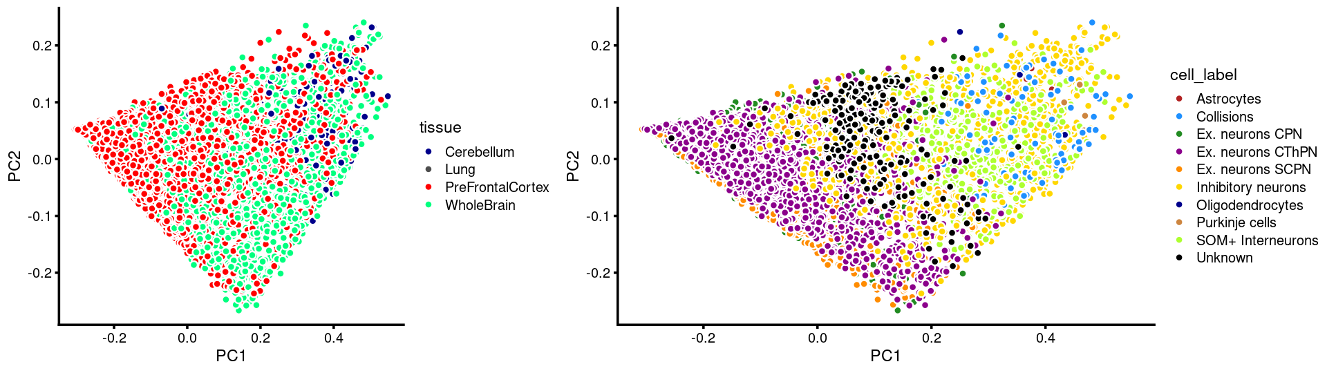
print(samples[intersect(rows.c14, which(samples$tissue == "Lung")),])
#                                       cell tissue tissue.replicate cluster
# 22109 TCCGCGAATAGGTAACTTACTGAGCGACGGCTCTGA   Lung      Lung2_62216      15
# 61277 TCTCGCGCTATTGCTGGACCTCCGACGGGTACTGAC   Lung      Lung2_62216       5
#       subset_cluster   tsne_1    tsne_2 subset_tsne1 subset_tsne2
# 22109              2 -1.07335 -12.29793    -8.494056    -4.764539
# 61277              2 -1.77437 -23.62355     4.220333     2.583797
#                          id         cell_label cluster_kmeans
# 22109 clusters_15.cluster_2 Inhibitory neurons            c14
# 61277  clusters_5.cluster_2   Ex. neurons SCPN            c14
PCA plots
Plot PCs of the topic proportions.
p.pca1.1 <- pca_plot(fit_multinom,pcs = 1:2,fill = "none")
p.pca1.2 <- pca_plot(fit_multinom,pcs = 3:4,fill = "none")
p.pca1.3 <- pca_plot(fit_multinom,pcs = 5:6,fill = "none")
p.pca1.4 <- pca_plot(fit_multinom,pcs = 7:8,fill = "none")
p.pca1.5 <- pca_plot(fit_multinom,pcs = 9:10,fill = "none")
p.pca1.6 <- pca_plot(fit_multinom,pcs = 11:12,fill = "none")

plot_grid(p.pca1.1,p.pca1.2,p.pca1.3,p.pca1.4,p.pca1.5,p.pca1.6)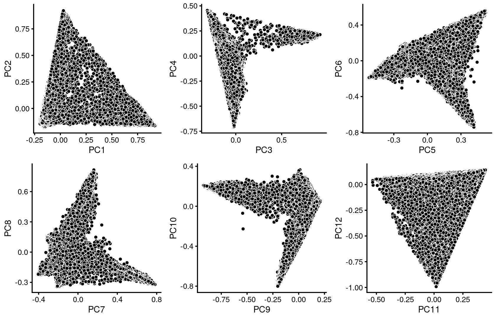
| Version | Author | Date |
|---|---|---|
| a38788b | kevinlkx | 2020-10-20 |
Some of the structure is more evident from “hexbin” plots showing the density of the points.
breaks <- c(0,1,5,10,100,Inf)
p.pca2.1 <- pca_hexbin_plot(fit_multinom, pcs = 1:2, breaks = breaks) + guides(fill = "none")
p.pca2.2 <- pca_hexbin_plot(fit_multinom, pcs = 3:4, breaks = breaks) + guides(fill = "none")
p.pca2.3 <- pca_hexbin_plot(fit_multinom, pcs = 5:6, breaks = breaks) + guides(fill = "none")
p.pca2.4 <- pca_hexbin_plot(fit_multinom, pcs = 7:8, breaks = breaks) + guides(fill = "none")
p.pca2.5 <- pca_hexbin_plot(fit_multinom, pcs = 9:10, breaks = breaks) + guides(fill = "none")
p.pca2.6 <- pca_hexbin_plot(fit_multinom, pcs = 11:12, breaks = breaks) + guides(fill = "none")

plot_grid(p.pca2.1,p.pca2.2,p.pca2.3,p.pca2.4,p.pca2.5,p.pca2.6)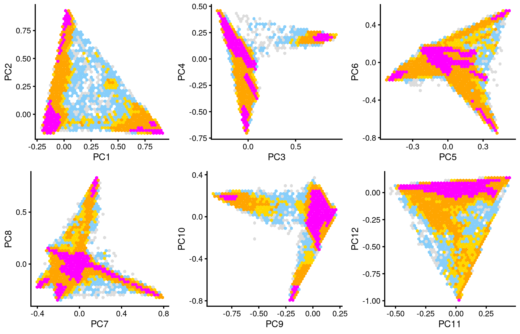
| Version | Author | Date |
|---|---|---|
| a38788b | kevinlkx | 2020-10-20 |
Layer the tissue and cell labels onto the PC plots
PCs 1 and 2:
p.pca3.1 <- labeled_pca_plot(fit,1:2,samples$tissue,font_size = 7,
                       colors = colors_tissues, legend_label = "tissue")
p.pca3.2 <- labeled_pca_plot(fit,1:2,samples$cell_label,font_size = 7,
                        legend_label = "cell_label")
plot_grid(p.pca3.1,p.pca3.2,rel_widths = c(8,11))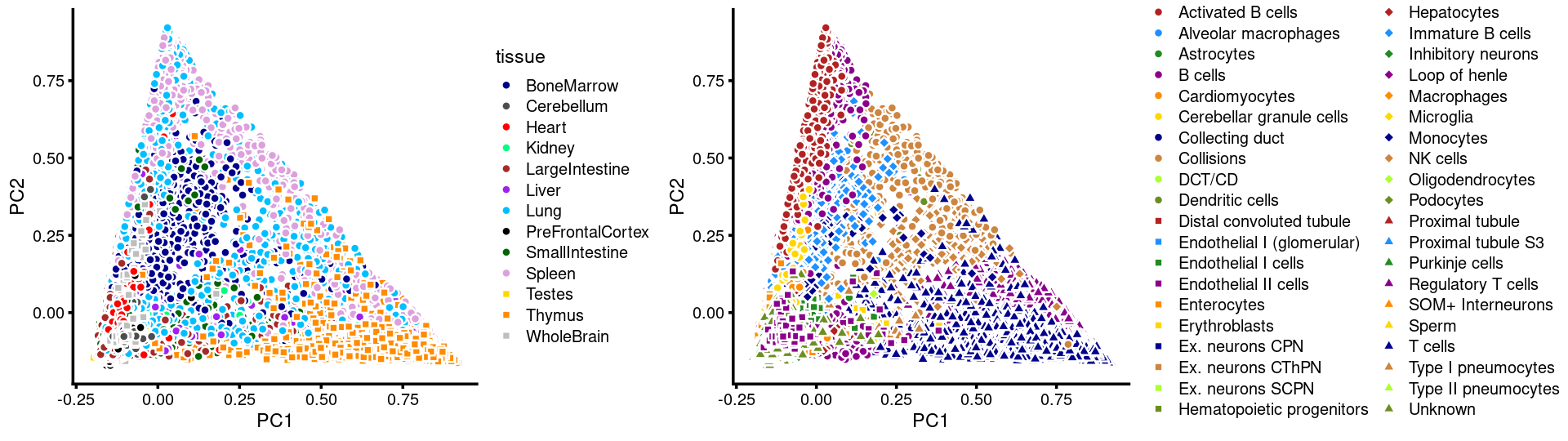
PCs 3 and 4:
p.pca3.3 <- labeled_pca_plot(fit,3:4,samples$tissue,font_size = 7,
                        colors = colors_tissues, legend_label = "tissue")
p.pca3.4 <- labeled_pca_plot(fit,3:4,samples$cell_label,font_size = 7,
                        legend_label = "cell_label")
plot_grid(p.pca3.3,p.pca3.4,rel_widths = c(8,11))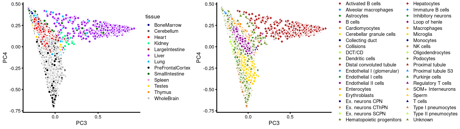
PCs 5 and 6:
p.pca3.5 <- labeled_pca_plot(fit,5:6,samples$tissue,font_size = 7,
                       colors = colors_tissues, legend_label = "tissue")
p.pca3.6 <- labeled_pca_plot(fit,5:6,samples$cell_label,font_size = 7,
                        legend_label = "cell_label")
plot_grid(p.pca3.5,p.pca3.6,rel_widths = c(8,11))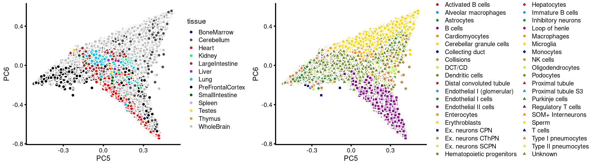
PCs 7 and 8:
p.pca3.7 <- labeled_pca_plot(fit,7:8,samples$tissue,font_size = 7,
                       colors = colors_tissues, legend_label = "tissue")
p.pca3.8 <- labeled_pca_plot(fit,7:8,samples$cell_label,font_size = 7,
                        legend_label = "cell_label")
plot_grid(p.pca3.7,p.pca3.8,rel_widths = c(8,11))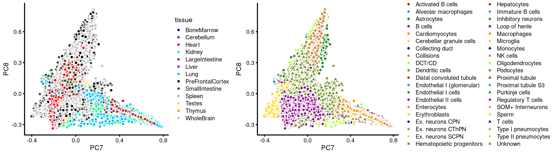
PCs 9 and 10:
p.pca3.9 <- labeled_pca_plot(fit,9:10,samples$tissue,font_size = 7,
                       colors = colors_tissues, legend_label = "tissue")
p.pca3.10 <- labeled_pca_plot(fit,9:10,samples$cell_label,font_size = 7,
                        legend_label = "cell_label")
plot_grid(p.pca3.9,p.pca3.10,rel_widths = c(8,11))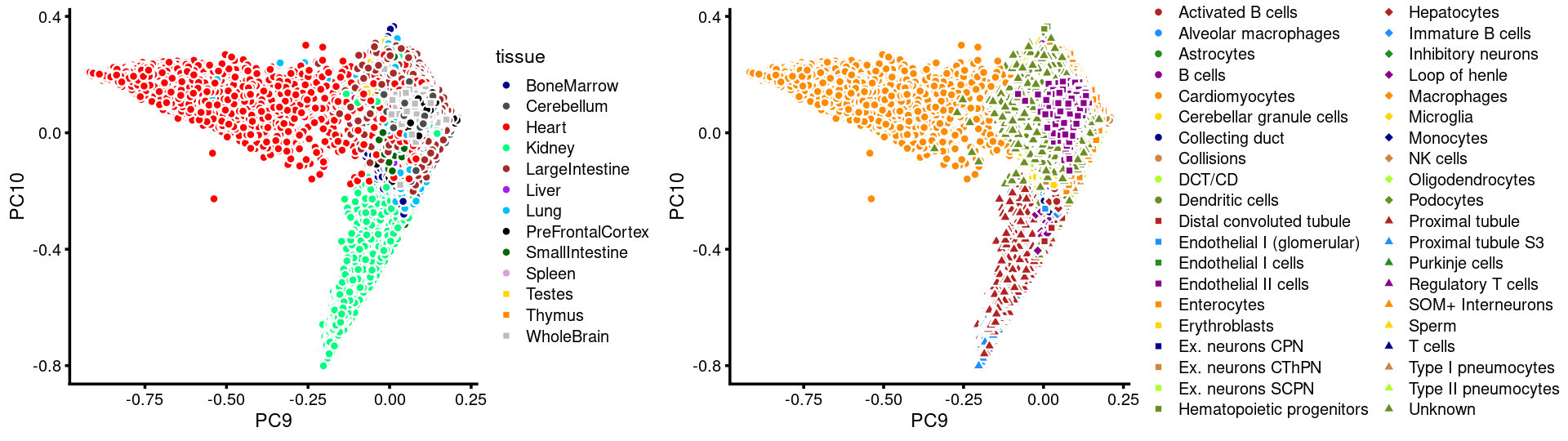
PCs 11 and 12:
p.pca3.11 <- labeled_pca_plot(fit,11:12,samples$tissue,font_size = 7,
                       legend_label = "tissue")
p.pca3.12 <- labeled_pca_plot(fit,11:12,samples$cell_label,font_size = 7,
                        legend_label = "cell_label")
plot_grid(p.pca3.11,p.pca3.12,rel_widths = c(8,11))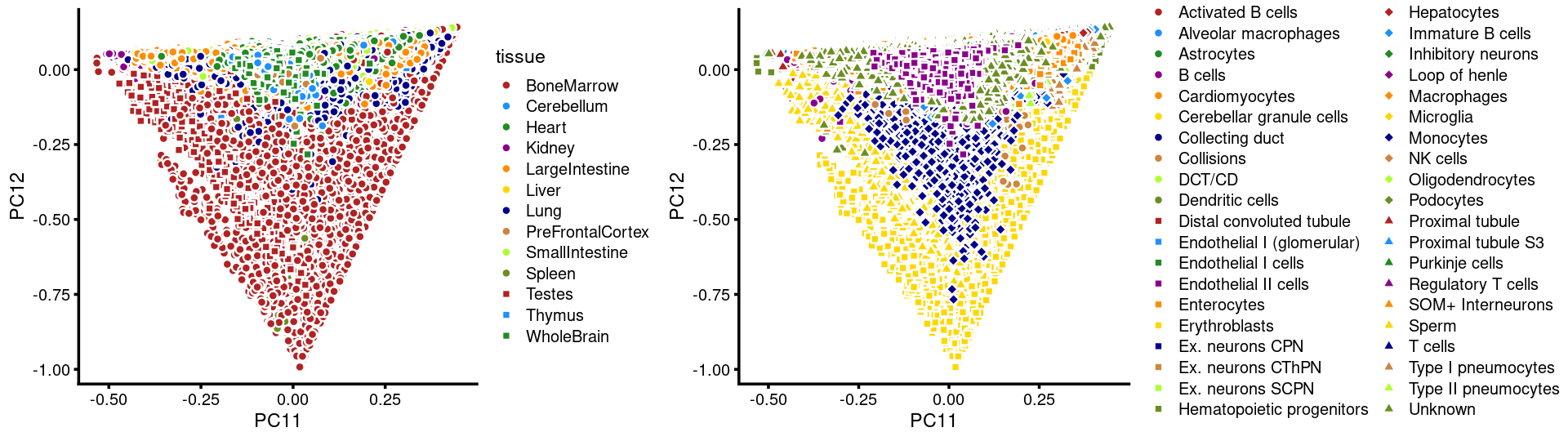
| Version | Author | Date |
|---|---|---|
| a38788b | kevinlkx | 2020-10-20 |
The clusters defined by k-means on topic proportions reasonably identify the clusters shown in the PCA hexbin plots (below).
p.pca.4.1 <- labeled_pca_plot(fit,1:2,samples$cluster_kmeans,font_size = 7,
                       legend_label = "cluster_kmeans")
p.pca.4.2 <- labeled_pca_plot(fit,3:4,samples$cluster_kmeans,font_size = 7,
                       legend_label = "cluster_kmeans")
p.pca.4.3 <- labeled_pca_plot(fit,5:6,samples$cluster_kmeans,font_size = 7,
                       legend_label = "cluster_kmeans")
p.pca.4.4 <- labeled_pca_plot(fit,7:8,samples$cluster_kmeans,font_size = 7,
                       legend_label = "cluster_kmeans")
p.pca.4.5 <- labeled_pca_plot(fit,9:10,samples$cluster_kmeans,font_size = 7,
                       legend_label = "cluster_kmeans")
p.pca.4.6 <- labeled_pca_plot(fit,11:12,samples$cluster_kmeans,font_size = 7,
                       legend_label = "cluster_kmeans")
plot_grid(p.pca.4.1,p.pca.4.2,p.pca.4.3,p.pca.4.4,p.pca.4.5,p.pca.4.6)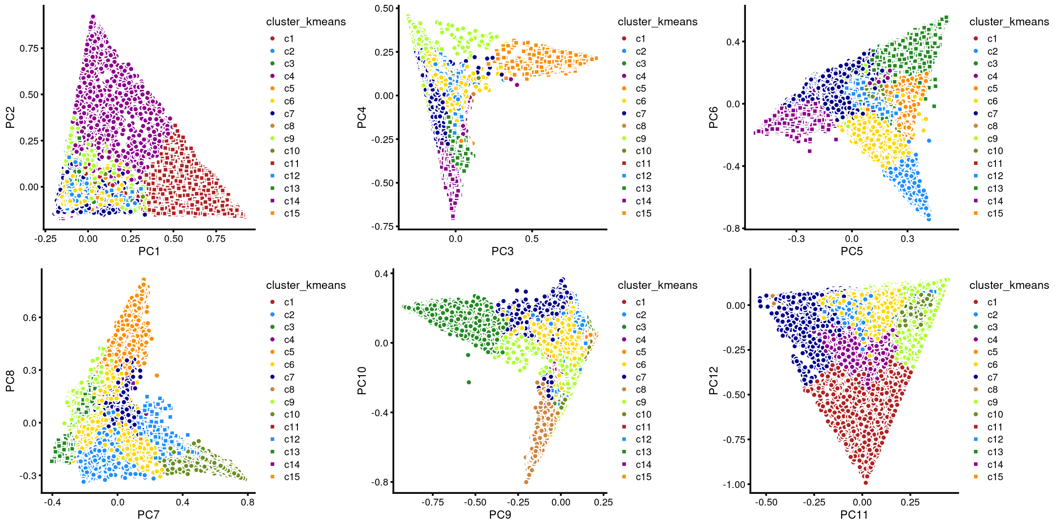
sessionInfo()
# R version 3.6.1 (2019-07-05)
# Platform: x86_64-pc-linux-gnu (64-bit)
# Running under: Scientific Linux 7.4 (Nitrogen)
#
# Matrix products: default
# BLAS/LAPACK: /software/openblas-0.2.19-el7-x86_64/lib/libopenblas_haswellp-r0.2.19.so
#
# locale:
#  [1] LC_CTYPE=en_US.UTF-8       LC_NUMERIC=C
#  [3] LC_TIME=en_US.UTF-8        LC_COLLATE=en_US.UTF-8
#  [5] LC_MONETARY=en_US.UTF-8    LC_MESSAGES=en_US.UTF-8
#  [7] LC_PAPER=en_US.UTF-8       LC_NAME=C
#  [9] LC_ADDRESS=C               LC_TELEPHONE=C
# [11] LC_MEASUREMENT=en_US.UTF-8 LC_IDENTIFICATION=C
#
# attached base packages:
# [1] stats     graphics  grDevices utils     datasets  methods   base
#
# other attached packages:
# [1] RColorBrewer_1.1-2 plyr_1.8.6         fastTopics_0.4-29  cowplot_1.1.1
# [5] ggplot2_3.3.3      dplyr_1.0.3        Matrix_1.2-18      workflowr_1.6.2
#
# loaded via a namespace (and not attached):
#  [1] ggrepel_0.9.1      Rcpp_1.0.6         lattice_0.20-41    tidyr_1.1.2
#  [5] prettyunits_1.1.1  rprojroot_2.0.2    digest_0.6.27      R6_2.5.0
#  [9] MatrixModels_0.4-1 evaluate_0.14      coda_0.19-4        httr_1.4.2
# [13] pillar_1.4.7       rlang_0.4.10       progress_1.2.2     lazyeval_0.2.2
# [17] data.table_1.13.6  irlba_2.3.3        SparseM_1.78       hexbin_1.28.1
# [21] whisker_0.4        rmarkdown_2.6      labeling_0.4.2     Rtsne_0.15
# [25] stringr_1.4.0      htmlwidgets_1.5.3  munsell_0.5.0      compiler_3.6.1
# [29] httpuv_1.5.4       xfun_0.19          pkgconfig_2.0.3    mcmc_0.9-7
# [33] htmltools_0.5.1.1  tidyselect_1.1.0   tibble_3.0.6       quadprog_1.5-8
# [37] matrixStats_0.58.0 viridisLite_0.3.0  crayon_1.4.0       conquer_1.0.2
# [41] withr_2.4.1        later_1.1.0.1      MASS_7.3-53        grid_3.6.1
# [45] jsonlite_1.7.2     gtable_0.3.0       lifecycle_0.2.0    DBI_1.1.0
# [49] git2r_0.27.1       magrittr_2.0.1     scales_1.1.1       RcppParallel_5.0.2
# [53] stringi_1.5.3      farver_2.0.3       fs_1.3.1           promises_1.1.1
# [57] ellipsis_0.3.1     generics_0.1.0     vctrs_0.3.6        tools_3.6.1
# [61] glue_1.4.2         purrr_0.3.4        hms_1.0.0          yaml_2.2.1
# [65] colorspace_2.0-0   plotly_4.9.3       knitr_1.30         quantreg_5.83
# [69] MCMCpack_1.5-0