This reproducible R Markdown
analysis was created with workflowr (version
1.7.1). The Checks tab describes the reproducibility checks
that were applied when the results were created. The Past
versions tab lists the development history.
Great job! The global environment was empty. Objects defined in the
global environment can affect the analysis in your R Markdown file in
unknown ways. For reproduciblity it’s best to always run the code in an
empty environment.
The command set.seed(20260127) was run prior to running
the code in the R Markdown file. Setting a seed ensures that any results
that rely on randomness, e.g. subsampling or permutations, are
reproducible.
Great! You are using Git for version control. Tracking code development
and connecting the code version to the results is critical for
reproducibility.
The results in this page were generated with repository version
27b3161.
See the Past versions tab to see a history of the changes made
to the R Markdown and HTML files.
Note that you need to be careful to ensure that all relevant files for
the analysis have been committed to Git prior to generating the results
(you can use wflow_publish or
wflow_git_commit). workflowr only checks the R Markdown
file, but you know if there are other scripts or data files that it
depends on. Below is the status of the Git repository when the results
were generated:
Note that any generated files, e.g. HTML, png, CSS, etc., are not
included in this status report because it is ok for generated content to
have uncommitted changes.
These are the previous versions of the repository in which changes were
made to the R Markdown
(analysis/cups_and_skulls_analysis.Rmd) and HTML
(docs/cups_and_skulls_analysis.html) files. If you’ve
configured a remote Git repository (see ?wflow_git_remote),
click on the hyperlinks in the table below to view the files as they
were in that past version.
Add data dictionary worksheet and chamber space analysis
How to Use This Analysis
THIS IS A TEMPLATE that you’ll customize as you
complete your data dictionaries.
What You Need to Do:
Complete data/period_dictionary.csv:
Assign chronological order to each period (1 = earliest, higher =
latest)
For range periods (e.g., “LHIIA-LHIIIB”), identify the earliest and
latest components
See analysis/data_dictionary.Rmd for detailed
instructions
Complete
data/tomb_type_dictionary.csv:
Decide how to rank the 5 tomb types (Tholos, Chamber Tomb, Cist
Grave, Pit Grave, Other)
Choose: by complexity, labor investment, or frequency
See analysis/data_dictionary.Rmd for guidance
Enable the Dictionary Loading Code:
Once dictionaries are complete, find the “Import and Process Data
Dictionaries” section
Change eval=FALSE to eval=TRUE
This activates the ordinal factors and enables temporal/complexity
analyses
What This Analysis Will Show (Once Dictionaries Are Complete):
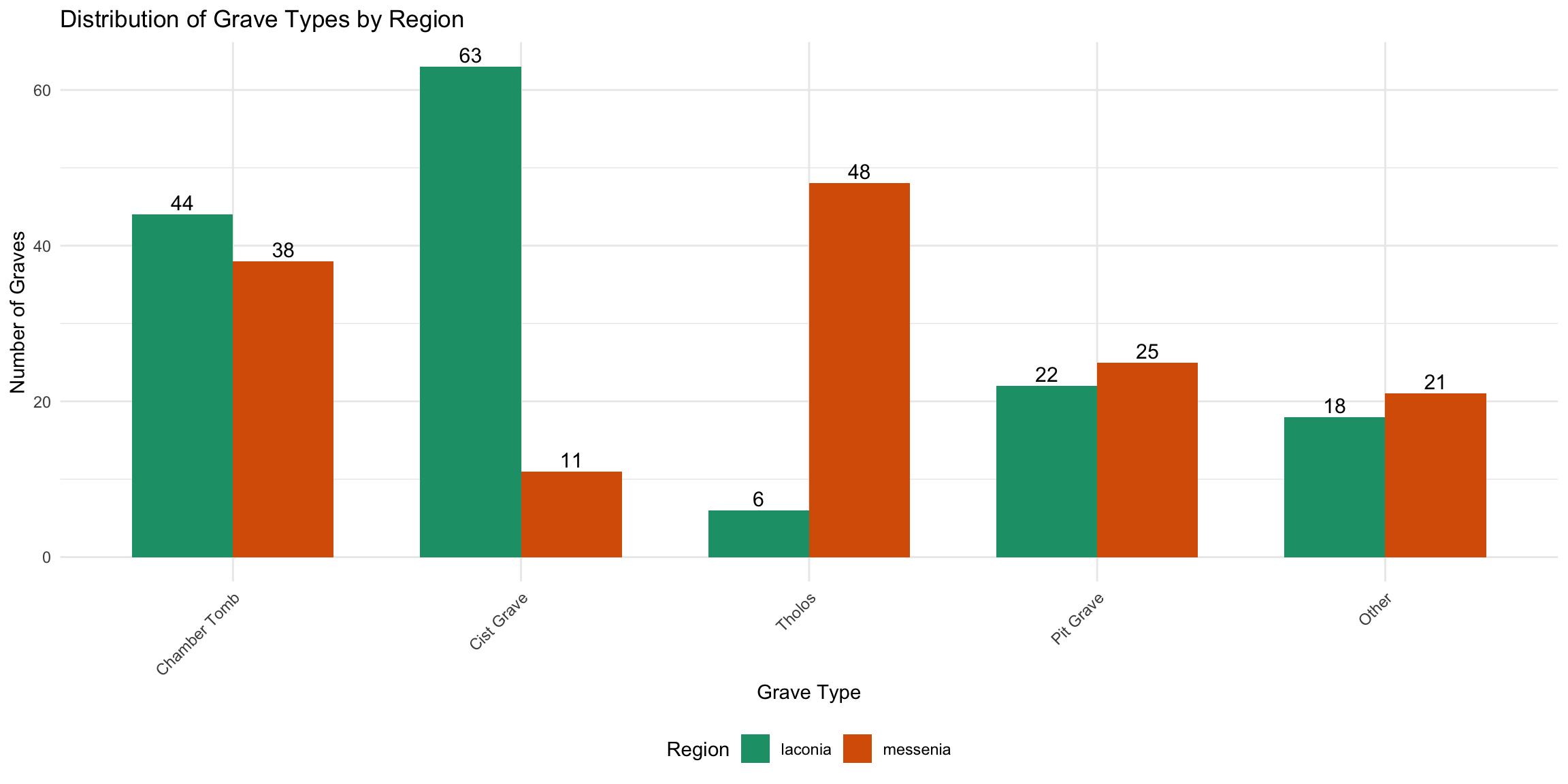
Distribution comparisons between Laconia and
Messenia
Temporal trends in drinking vessel deposition
across periods
Complexity patterns in tomb types and burial
practices
Regional differences in how graves are used
Relationships between chamber size, drinking
vessels, and skeletal remains
Your decisions in the dictionaries will shape these findings — so
think carefully about your ranking logic!
Introduction
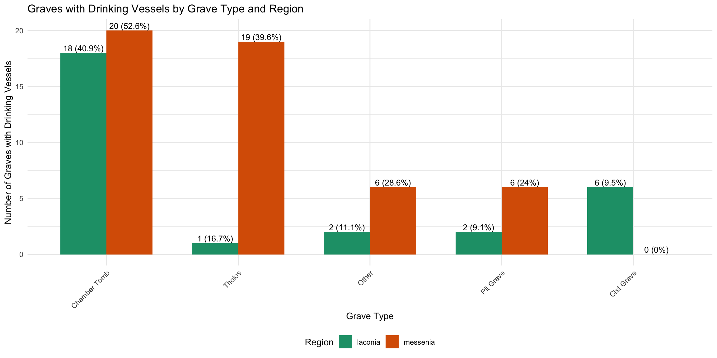
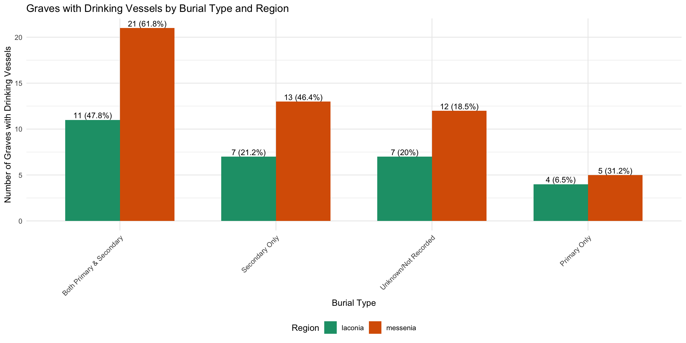
This analysis examines the relationship between drinking vessels and
human skeletal remains in Laconian and Messinian tholos and chamber
tombs. The data focuses on grave contexts where drinking vessels are
recorded alongside information about primary and secondary burials.
YOU CAN EDIT THIS SECTION: Customize colors for the
analyses. Edit the hex codes below to use your preferred colors.
All plots throughout this analysis will use these colors, so if you
change them here, the change applies everywhere automatically.
Color choices affect: - Regional comparisons
(Laconia vs Messenia) - Visualization clarity and accessibility - How
different variables stand out in plots
# Set your color palette here
colors <- list(
  laconia = "#1B9E77",      # Laconia color (default: teal/green)
  messenia = "#D95F02",     # Messenia color (default: orange)
  drinking_vessel = "#7570B3",  # Drinking vessels (default: purple)
  skulls = "#E7298A",        # Skulls (default: pink)
  background = "#FFFFCC"     # Background/neutral (default: light yellow)
)

# These colors will be used throughout all plots
# Change the hex codes to your preferred colors
Load Data
# Load the CSV data
data_path <- here::here("data", "laconia_messinia_cups_skulls.csv")
cups_skulls <- read_csv(data_path)
Rows: 296 Columns: 14
── Column specification ────────────────────────────────────────────────────────
Delimiter: ","
chr (11): Grave ID, site, type, period, secondary, primary, dimensions, orie...
dbl  (3): drinking vessel number, skulls number, area of chamber estimated

ℹ Use `spec()` to retrieve the full column specification for this data.
ℹ Specify the column types or set `show_col_types = FALSE` to quiet this message.
NOTE: The code below simplifies the complex grave
type names into broader categories. If you want to group grave types
differently, you can edit the case_when() statements in
this chunk. For example, you might want to keep “Pit Grave” and “Cist
Grave” separate, or group them together.
cups_skulls_clean <- cups_skulls %>%
  # Clean column names
  janitor::clean_names() %>%

  # Trim whitespace from character columns
  mutate(across(where(is.character), str_trim)) %>%

  # Standardize yes/no values in drinking vessel column
  mutate(
    has_drinking_vessel = case_when(
      tolower(drinking_vessel) == "yes" ~ TRUE,
      tolower(drinking_vessel) == "no" ~ FALSE,
      TRUE ~ NA
    ),
    has_remains = case_when(
      tolower(remains) == "yes" ~ TRUE,
      tolower(remains) == "no" ~ FALSE,
      TRUE ~ NA
    ),
    primary_burial = case_when(
      tolower(primary) == "present" ~ TRUE,
      tolower(primary) == "absent" ~ FALSE,
      TRUE ~ NA
    ),
    secondary_burial = case_when(
      tolower(secondary) == "present" ~ TRUE,
      tolower(secondary) == "absent" ~ FALSE,
      TRUE ~ NA
    )
  ) %>%

  # Create burial category
  mutate(
    burial_category = case_when(
      primary_burial & secondary_burial ~ "Both Primary & Secondary",
      primary_burial & !secondary_burial ~ "Primary Only",
      !primary_burial & secondary_burial ~ "Secondary Only",
      TRUE ~ "Unknown/Not Recorded"
    )
  ) %>%

  # Simplify grave type
  # ** YOU CAN CUSTOMIZE THIS SECTION **
  # If you want different groupings, edit the patterns here
  # Current grouping is based on archaeological complexity
  mutate(
    grave_type_simple = case_when(
      str_detect(tolower(type), "tholos") ~ "Tholos",
      str_detect(tolower(type), "chamber") ~ "Chamber Tomb",
      str_detect(tolower(type), "cist") ~ "Cist Grave",
      str_detect(tolower(type), "pit") ~ "Pit Grave",
      str_detect(tolower(type), "dromos") ~ "Dromos Only",
      TRUE ~ "Other"
    )
  )

# Show cleaned data structure
glimpse(cups_skulls_clean)
What this enables: - Testing whether drinking vessel
deposition changes over time - Comparing tomb complexity with burial
practices - Temporal and complexity-based statistical models
After dictionaries are complete, this section will
load and apply ordinal rankings:
# NOTE: Set eval=TRUE once the student has completed the dictionaries

# Load period dictionary
period_dict <- read_csv(here::here("data", "period_dictionary.csv"))

# Load tomb type dictionary
tomb_dict <- read_csv(here::here("data", "tomb_type_dictionary.csv"))

# Join period dictionary and extract period components
cups_skulls_clean <- cups_skulls_clean %>%
  left_join(
    period_dict %>% select(period_code, chronological_order, earliest_component, latest_component),
    by = c("period" = "period_code")
  ) %>%

  # Get ordinal values for earliest component
  left_join(
    period_dict %>% select(period_code, chronological_order) %>% rename(start_order = chronological_order),
    by = c("earliest_component" = "period_code")
  ) %>%

  # Get ordinal values for latest component
  left_join(
    period_dict %>% select(period_code, chronological_order) %>% rename(end_order = chronological_order),
    by = c("latest_component" = "period_code")
  ) %>%

  # For single periods (where start = end), use that value
  # For ranges, create midpoint
  mutate(
    period_start_order = start_order,
    period_end_order = end_order,
    period_midpoint_order = (start_order + end_order) / 2
  )

# Join tomb type dictionary
cups_skulls_clean <- cups_skulls_clean %>%
  left_join(
    tomb_dict %>% select(tomb_type, tomb_type_order),
    by = c("grave_type_simple" = "tomb_type")
  ) %>%

  # Convert to ordered factors
  mutate(
    tomb_type_ordered = factor(
      grave_type_simple,
      levels = arrange(tomb_dict, tomb_type_order) %>% pull(tomb_type),
      ordered = TRUE
    ),
    period_ordered = factor(
      period,
      levels = arrange(period_dict, chronological_order) %>% pull(period_code),
      ordered = TRUE
    )
  )

cat("✓ Dictionaries successfully loaded and applied!\n")
cat("New columns created:\n")
cat("  - period_start_order: chronological order of earliest period component\n")
cat("  - period_end_order: chronological order of latest period component\n")
cat("  - period_midpoint_order: midpoint between start and end\n")
cat("  - tomb_type_ordered: ordered factor for tomb types\n")
cat("  - period_ordered: ordered factor for periods\n")
Data Overview
Basic Statistics
These are descriptive statistics of your dataset. They won’t change
based on your dictionaries, but they provide context for all analyses
below.
HOW YOUR CHOICES AFFECT THIS: - The groupings in the
“Data Cleaning” section determine what you see here - If you edit
grave_type_simple to create different categories, these
plots will change - Once you complete
tomb_type_dictionary.csv, you can run additional analyses
on tomb complexity
cat(" - Skull counts recorded in", sum(!is.na(cups_skulls_clean$skulls_number)), "graves\n\n")
- Skull counts recorded in 83 graves
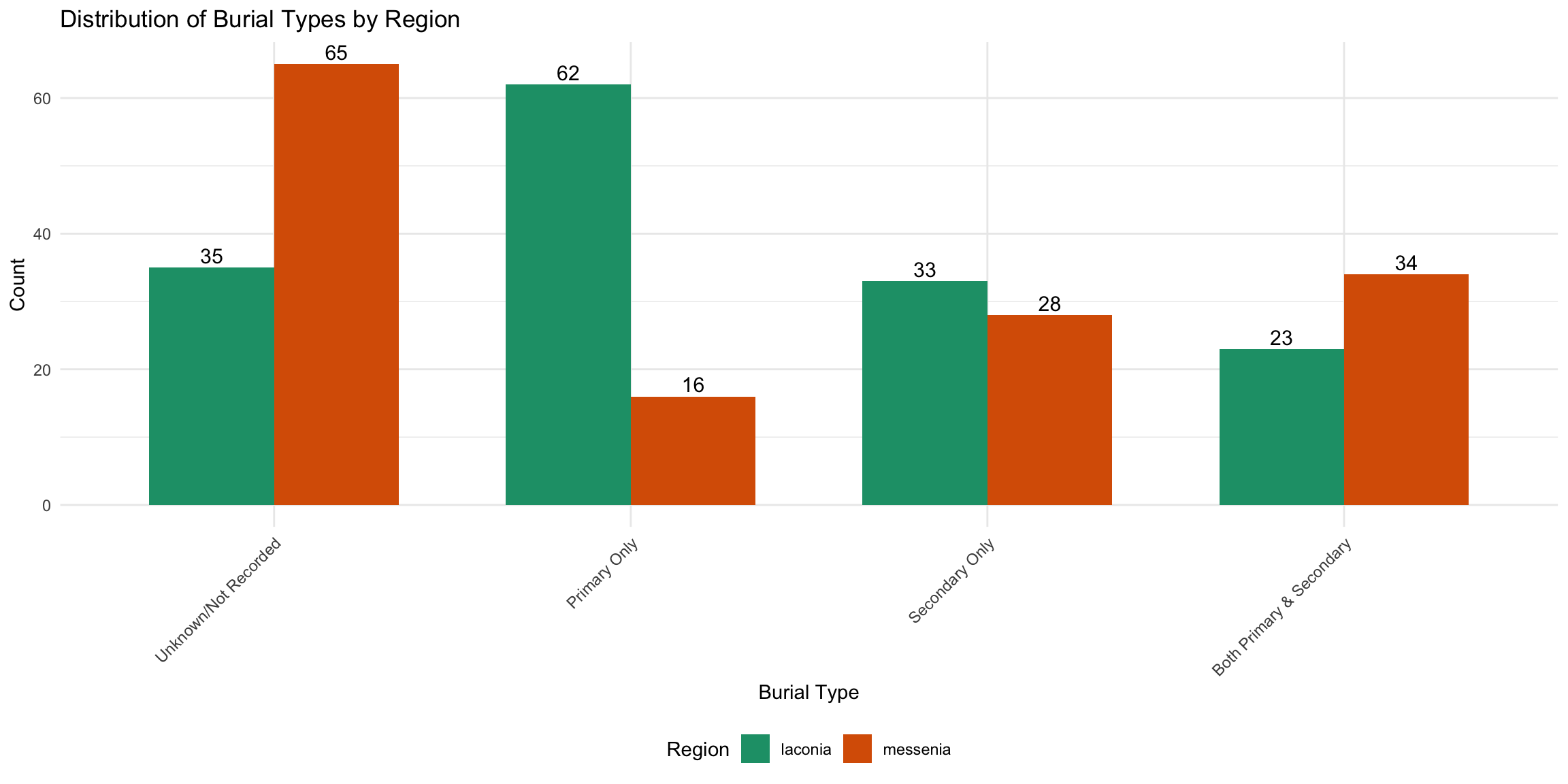
cat("3. Burial Type Association:\n")
3. Burial Type Association:
burial_counts <- cups_skulls_clean %>%
  count(burial_category) %>%
  arrange(desc(n))
for (i in 1:nrow(burial_counts)) {
  cat("   -", burial_counts$burial_category[i], ":", burial_counts$n[i], "graves\n")
}
   - Unknown/Not Recorded : 100 graves
   - Primary Only : 78 graves
   - Secondary Only : 61 graves
   - Both Primary & Secondary : 57 graves
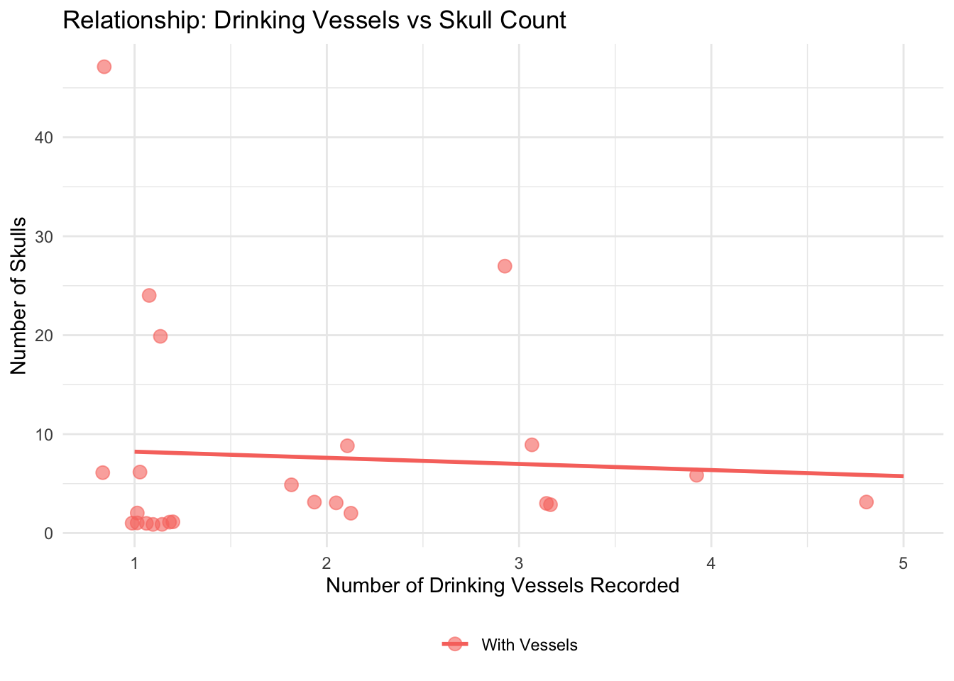
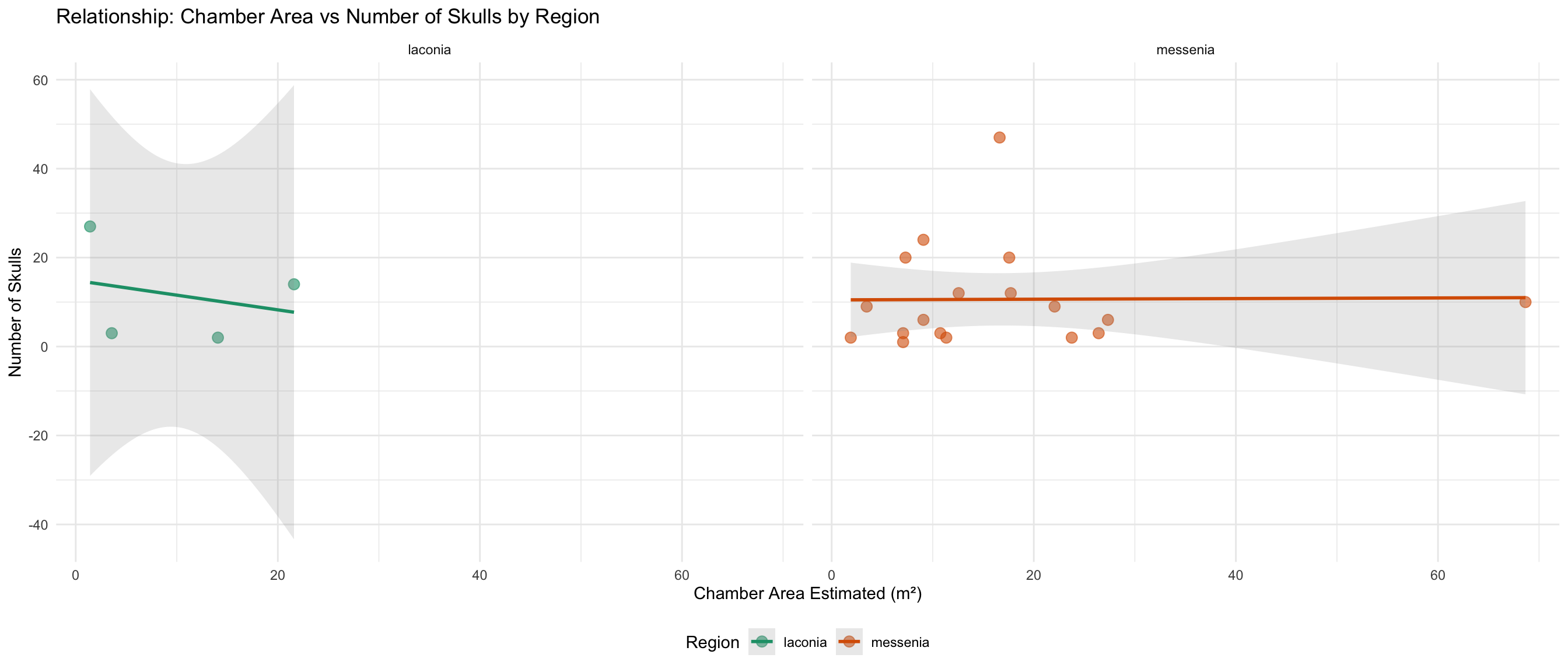
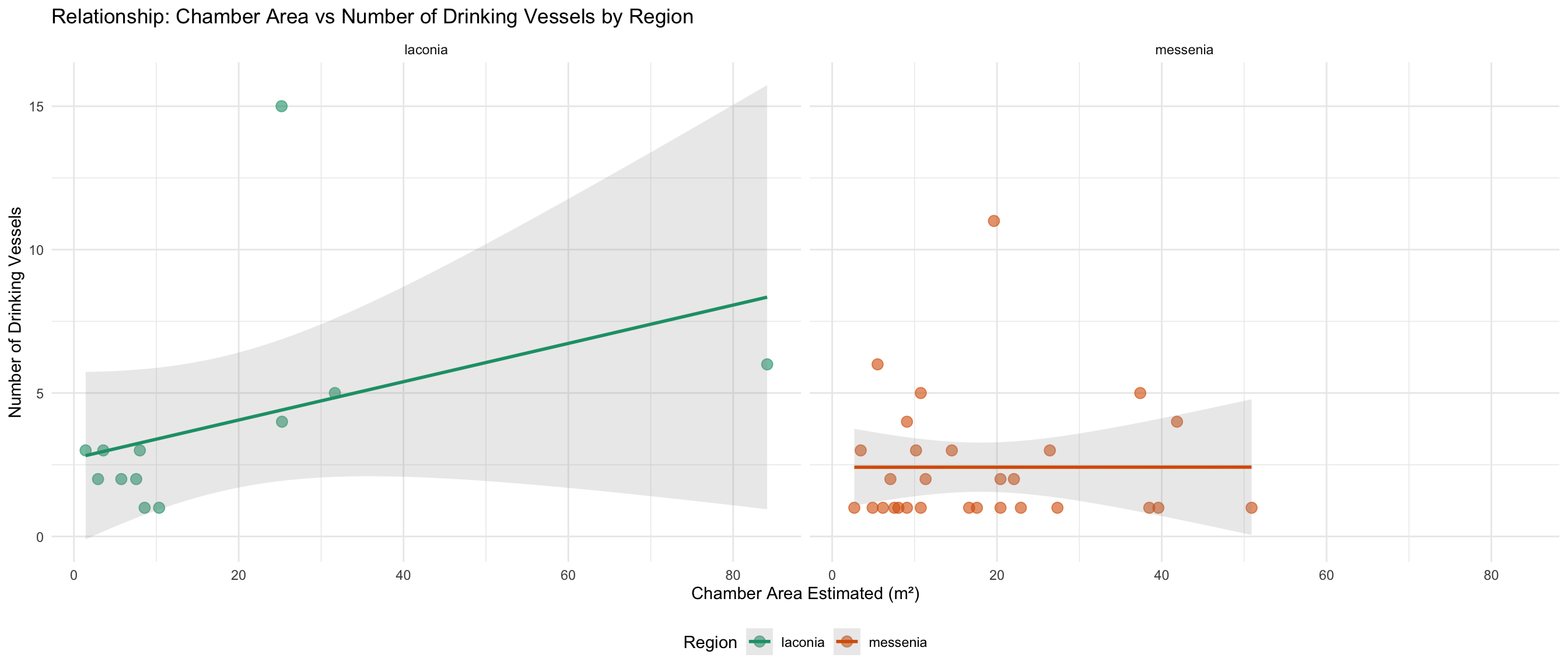
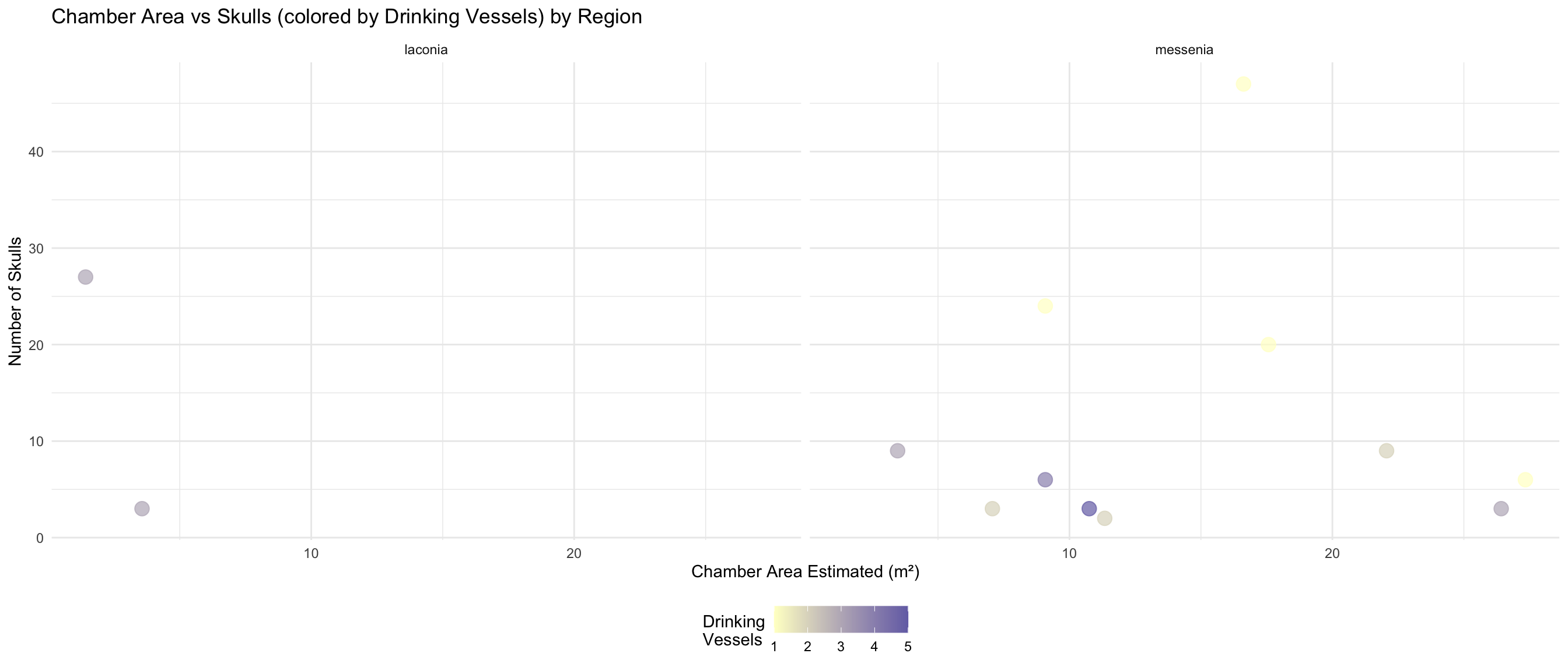
Chamber Space and Burial Goods
Do larger chambers have more skulls and drinking vessels?
This section explores whether the estimated chamber area relates to
the number of skulls and drinking vessels found.
HOW YOUR PERIOD DICTIONARY WILL ENHANCE THIS: - Once
you complete period_dictionary.csv and enable the
dictionary loading code, we can add temporal layers - You’ll be able to
see if these relationships change across periods - Time-based patterns
can reveal ritual practice evolution
Data Availability
space_analysis_data <- cups_skulls_clean %>%
  filter(!is.na(area_of_chamber_estimated))

cat("Graves with chamber area estimated:", nrow(space_analysis_data), "\n")
Graves with chamber area estimated: 99
cat("Graves with area AND skull count:", sum(!is.na(space_analysis_data$skulls_number)), "\n")
Graves with area AND skull count: 22
cat("Graves with area AND vessel count:", sum(!is.na(space_analysis_data$drinking_vessel_number)), "\n\n")
Graves with area AND vessel count: 41
# Summary statistics for chamber area
cat("Chamber Area Summary (m²):\n")