Analyses
Tina Lasisi
2023-03-23 16:39:57
Last updated: 2023-03-23
Checks: 7 0
Knit directory: PODFRIDGE/
This reproducible R Markdown analysis was created with workflowr (version 1.7.0). The Checks tab describes the reproducibility checks that were applied when the results were created. The Past versions tab lists the development history.
Great! Since the R Markdown file has been committed to the Git repository, you know the exact version of the code that produced these results.
Great job! The global environment was empty. Objects defined in the global environment can affect the analysis in your R Markdown file in unknown ways. For reproduciblity it’s best to always run the code in an empty environment.
The command set.seed(20230302) was run prior to running
the code in the R Markdown file. Setting a seed ensures that any results
that rely on randomness, e.g. subsampling or permutations, are
reproducible.
Great job! Recording the operating system, R version, and package versions is critical for reproducibility.
Nice! There were no cached chunks for this analysis, so you can be confident that you successfully produced the results during this run.
Great job! Using relative paths to the files within your workflowr project makes it easier to run your code on other machines.
Great! You are using Git for version control. Tracking code development and connecting the code version to the results is critical for reproducibility.
The results in this page were generated with repository version b24ae94. See the Past versions tab to see a history of the changes made to the R Markdown and HTML files.
Note that you need to be careful to ensure that all relevant files for
the analysis have been committed to Git prior to generating the results
(you can use wflow_publish or
wflow_git_commit). workflowr only checks the R Markdown
file, but you know if there are other scripts or data files that it
depends on. Below is the status of the Git repository when the results
were generated:
Ignored files:
    Ignored:    .DS_Store
    Ignored:    .Rhistory
    Ignored:    .Rproj.user/
    Ignored:    data/.DS_Store
Note that any generated files, e.g. HTML, png, CSS, etc., are not included in this status report because it is ok for generated content to have uncommitted changes.
These are the previous versions of the repository in which changes were
made to the R Markdown (analysis/analyses.Rmd) and HTML
(docs/analyses.html) files. If you’ve configured a remote
Git repository (see ?wflow_git_remote), click on the
hyperlinks in the table below to view the files as they were in that
past version.
| File | Version | Author | Date | Message |
|---|---|---|---|---|
| Rmd | b24ae94 | Tina Lasisi | 2023-03-23 | Generating figures across variable combos |
| Rmd | 6605057 | Tina Lasisi | 2023-03-20 | Update parameters for generations |
| html | 6605057 | Tina Lasisi | 2023-03-20 | Update parameters for generations |
| html | 5f805fe | Tina Lasisi | 2023-03-06 | Build site. |
| Rmd | 5106bab | Tina Lasisi | 2023-03-06 | add analyses |
| html | c3948af | Tina Lasisi | 2023-03-05 | Build site. |
| html | f02bc38 | Tina Lasisi | 2023-03-03 | Build site. |
| html | c9130d5 | Tina Lasisi | 2023-03-03 | wflow_git_commit(all = TRUE) |
| html | a4a7d45 | Tina Lasisi | 2023-03-03 | Build site. |
| html | 00073fd | Tina Lasisi | 2023-03-03 | Build site. |
| html | 51ed5a6 | Tina Lasisi | 2023-03-03 | Build site. |
| Rmd | 13ed9ae | Tina Lasisi | 2023-03-03 | Publishing POPFORGE |
| html | 13ed9ae | Tina Lasisi | 2023-03-03 | Publishing POPFORGE |
# Load necessary packages
library(wesanderson) # for color palettes
library(tidyverse) #data wrangling etc
── Attaching packages ─────────────────────────────────────── tidyverse 1.3.2 ──
✔ ggplot2 3.4.0 ✔ purrr 0.3.5
✔ tibble 3.1.8 ✔ dplyr 1.0.10
✔ tidyr 1.2.1 ✔ stringr 1.5.0
✔ readr 2.1.3 ✔ forcats 0.5.2
── Conflicts ────────────────────────────────────────── tidyverse_conflicts() ──
✖ dplyr::filter() masks stats::filter()
✖ dplyr::lag() masks stats::lag()# Set path to the data file
path <- file.path(".", "data")
savepath <- file.path(".", "output")
# Set up vector for cousin degree
p <- c(1:8)
# Set up initial population size
N <- 76e6
# Set up vector of database sizes to test
DB.sizes <- c(1e6, 5e6, 10e6)
# Set color palette for graphs
my.cols <- wes_palette("Darjeeling1")# Read in data on US population sizes by year
US_pop <- read.csv(file.path(path,"est-pop-combo.csv"))
# Calculate number of grandparents by generation
# p_grandpar_gen <- 1950 - 30 * (p + 1)
p_grandpar_gen <- 1990 - 30 * (p + 1)
# Get population sizes by year for grandparents' generation
US_Ns <- US_pop %>%
filter(Year %in% p_grandpar_gen)
# Scale population size down by 50% (assumed number of potential parents) and 90% of those have children + set minimum for populations
#
# N <- US_Ns %>%
# mutate(across(!Year, ~ . * 0.5 * 0.9))
N <- US_Ns %>%
mutate(across(!Year, ~ case_when(. * 0.5 * 0.9 < 1e6 ~ 1e6,
TRUE ~ . * 0.5 * 0.9)))
# Set up vector of database sizes to test
DB.sizes <- c(1e6, 5e6, 10e6)
# Set color palette for graphs
my.cols <- wes_palette("Darjeeling1")# Calculate number of grandparents by generation
calc_grandparent_gen <- function(year, p = c(1:8)) {
grandparent_gen <- year - 30 * (p + 1)
return(grandparent_gen)
}
# Define a function to calculate final population sizes based on input data file and generation of grandparents
calc_final_N <- function(file_path, p_grandpar_gen) {
# Read in data on US population sizes by year
US_pop <- read.csv(file_path)
names(US_pop)[1] <- "Year"
# Get population sizes by year for grandparents' generation
US_Ns <- US_pop %>%
filter(Year %in% p_grandpar_gen)
# Scale population size down by 50% (assumed number of potential parents) and 90% of those have children + set minimum for populations
N <- US_Ns %>%
mutate(across(!Year, ~ case_when(. * 0.5 * 0.9 < 1e6 ~ 1e6,
TRUE ~ . * 0.5 * 0.9)))
return(N)
}
# get file
US_pop_fp <- file.path(path, "est-pop-combo.csv")
US_pop_coop_fp <- file.path(path, "US_popsize.csv")p_grandpar_gen <- calc_grandparent_gen(1990)
N <- calc_final_N(US_pop_fp, p_grandpar_gen)# Define the population sizes and names
populations <- N %>%
pivot_longer(-Year, names_to = "Population", values_to = "N")
# Create a ggplot object to visualize population sizes
pop_size_plot <- ggplot(populations, aes(x = Population, y = N)) +
geom_bar(stat = "identity", fill = "steelblue") +
labs(x = "Population", y = "Population size") +
theme_minimal() +
facet_wrap(~Year)
# Display the plot
print(pop_size_plot)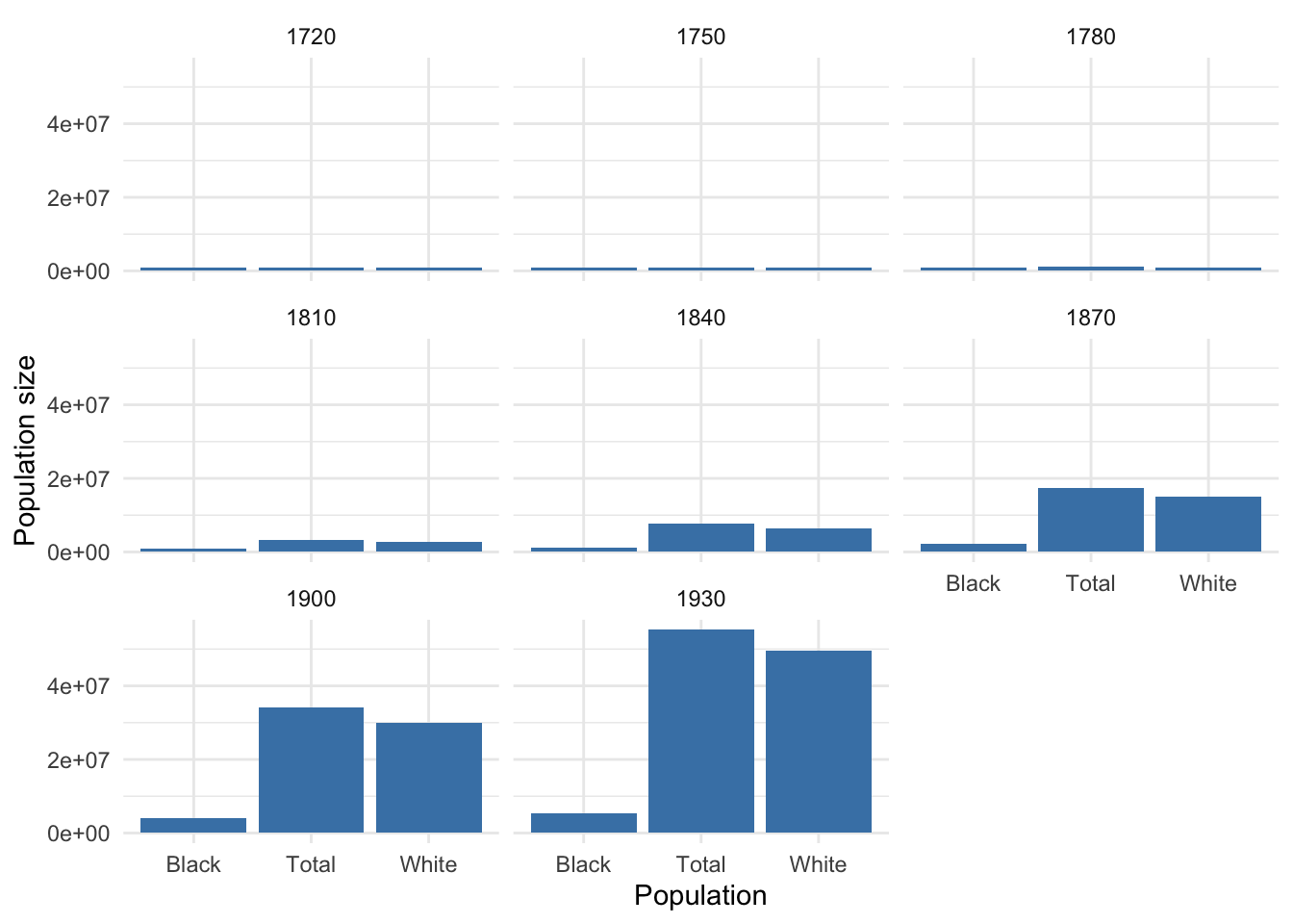
Probability of p-th degree cousin
library(wesanderson)
library(ggplot2)

# Function to calculate probabilities for finding a p-th degree cousin
calc_prob <- function(p, DB.size, N) {
  prob.no.rellys <- exp(-2^(2*p - 2) * DB.size / N)
  return(1 - prob.no.rellys)
}

# Function to calculate probabilities for different database fractions
calc_prob_db_frac <- function(p, DB.sizes, db.frac, N) {
  data <- data.frame(p = integer(), Population = character(), DB.size = double(), Probability = double(), Fraction = double())

  for (pop_name in names(N)) {
    for (i in 1:length(db.frac)) {
      for (j in 1:length(DB.sizes)) {
        DB.size <- DB.sizes[j] * db.frac[i]
        prob <- calc_prob(p, DB.size, N[[pop_name]])
        data <- rbind(data, data.frame(p = p, Population = rep(pop_name, length(p)), DB.size = rep(DB.sizes[j], length(p)), Probability = prob, Fraction = rep(db.frac[i], length(p))))
      }
    }
  }

  return(data)
}


# Function to generate ggplot object
ggplot_prob <- function(data, my.cols) {
  plot <- ggplot(data, aes(x = p, y = Probability, color = factor(DB.size), group = factor(DB.size))) +
    geom_point() +
    geom_line() +
    scale_color_manual(values = my.cols, name = "Database size (Millions)",
                       labels = format(unique(data$DB.size) / 1e6, dig = 1)) +
    labs(x = "p (degree of cousin)", y = "Probability of at least one p-th cousin in database") +
    theme_minimal() +
    facet_grid(Fraction ~ Population, labeller = labeller(Fraction = function(x) sprintf("%.0f%%", as.numeric(x) * 100)))

  return(plot)
}

# Set color palette for graphs
my.cols <- wes_palette("Darjeeling1")

# Define the population sizes and names
populations <- list(
  "European American" = N$White,
  "African American" = N$Black,
  "Total US" = N$Total
)

# Define the database sizes and fractions
DB.sizes <- c(1e6, 5e6, 10e6)
db.frac <- c(0.05, 0.8, 1)

# Calculate the probabilities for each population and database fraction
prob_data <- calc_prob_db_frac(p, DB.sizes, db.frac, populations)

# Create and display the ggplot object
prob_plot <- ggplot_prob(prob_data, my.cols)
print(prob_plot)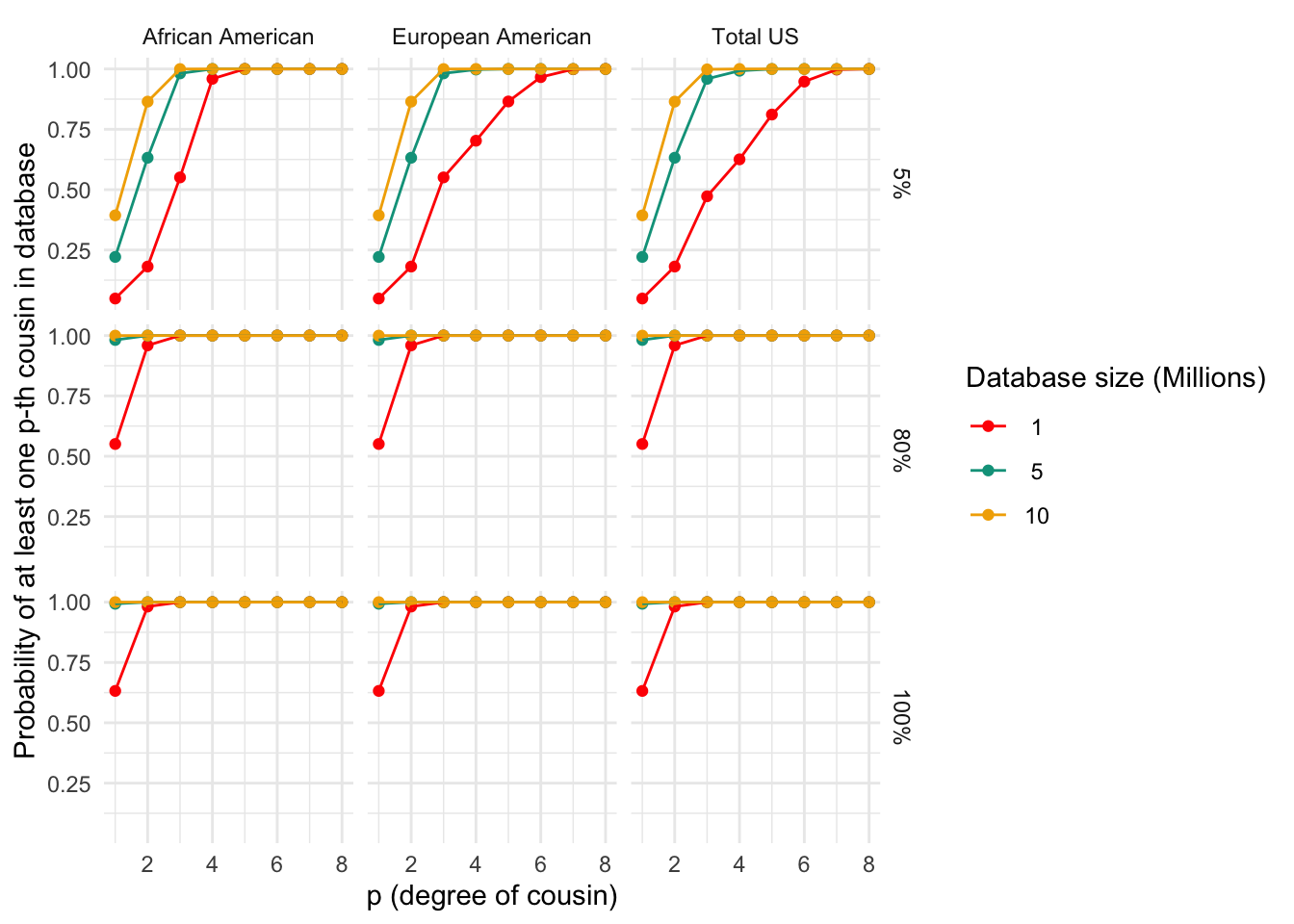
# Print the table of final probabilities
# print(prob_data)
# Function to generate ggplot object with populations in different colors
ggplot_prob_combined <- function(data, my.cols) {
plot <- ggplot(data, aes(x = p, y = Probability, color = Population, group = interaction(Population, factor(DB.size)))) +
geom_point() +
geom_line() +
scale_color_manual(values = my.cols, name = "Population") +
labs(x = "p (degree of cousin)", y = "Probability of at least one p-th cousin in database") +
theme_minimal() +
facet_grid(Fraction ~ factor(DB.size),
labeller = labeller(Fraction = function(x) sprintf("%.0f%%", as.numeric(x) * 100),
DB.size = function(x) sprintf("%gM", x / 1e6)))
function(x) formatC(x / 1e6, format = "f", digits = 0, big.mark = ",")
return(plot)
}
# Set color palette for graphs
my.cols <- wes_palette("Darjeeling1", n = 3, type = "continuous")
# Create and display the ggplot object with populations in different colors
prob_combined_plot <- ggplot_prob_combined(prob_data, my.cols)
print(prob_combined_plot)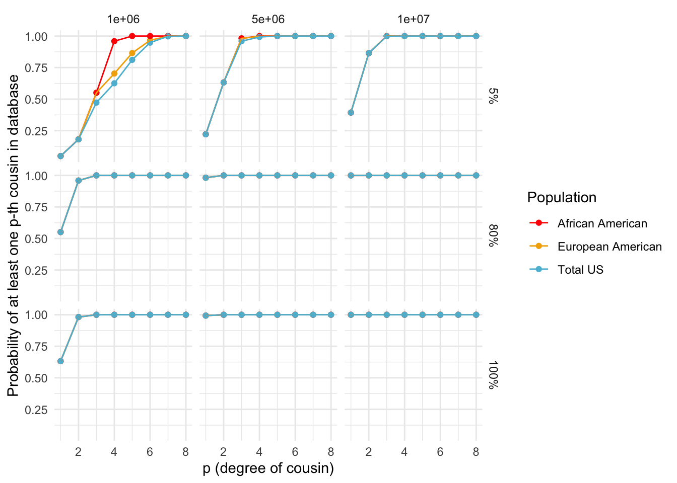
Number of p-th degree cousins
# Function to calculate the number of p-th degree cousins
calc_cousins <- function(p, DB.size, N) {
  num_cousins <- 4^(p) * DB.size / (N / 2)
  return(num_cousins)
}

# Function to calculate the number of p-th degree cousins for different database fractions
calc_cousins_db_frac <- function(p, DB.sizes, db.frac, N) {
  data <- data.frame(p = integer(), Population = as.character(), DB.size = double(), Cousins = double(), Fraction = double())

  for (pop_name in names(N)) {
    for (i in 1:length(db.frac)) {
      for (j in 1:length(DB.sizes)) {
        DB.size <- DB.sizes[j] * db.frac[i]
        cousins <- calc_cousins(p, DB.size, N[[pop_name]])
        data <- rbind(data, data.frame(p = p, Population = rep(pop_name, length(p)), DB.size = rep(DB.sizes[j], length(p)), Cousins = cousins, Fraction = rep(db.frac[i], length(p))))
      }
    }
  }

  return(data)
}

# Function to generate ggplot object
ggplot_cousins <- function(data, my.cols) {
  plot <- ggplot(data, aes(x = p, y = Cousins, color = factor(DB.size), group = factor(DB.size))) +
    geom_point() +
    geom_line() +
    scale_color_manual(values = my.cols, name = "Database size (Millions)", labels = c("1", "5", "10")) +
    labs(x = "p (degree of cousin)", y = "Number of p-th degree cousins in database") +
    theme_minimal() +
    facet_grid(Fraction ~ Population, labeller = labeller(Fraction = function(x) sprintf("%.0f%%", as.numeric(x) * 100), Population = c("European American" = "European American", "African American" = "African American", "Total US" = "Total US")))

  return(plot)
}

# Set up vector of database sizes to test
DB.sizes <- c(1e6, 5e6, 10e6)

# Define the database fractions
db.frac <- c(0.05, 0.8, 1)

# Define the population sizes and names
populations <- list(
  "European American" = N$White,
  "African American" = N$Black,
  "Total US" = N$Total
)

# Calculate the number of cousins for each population and database fraction
cousins_data <- calc_cousins_db_frac(p, DB.sizes, db.frac, populations)

# Create and display the ggplot object
cousins_plot <- ggplot_cousins(cousins_data, my.cols)
print(cousins_plot)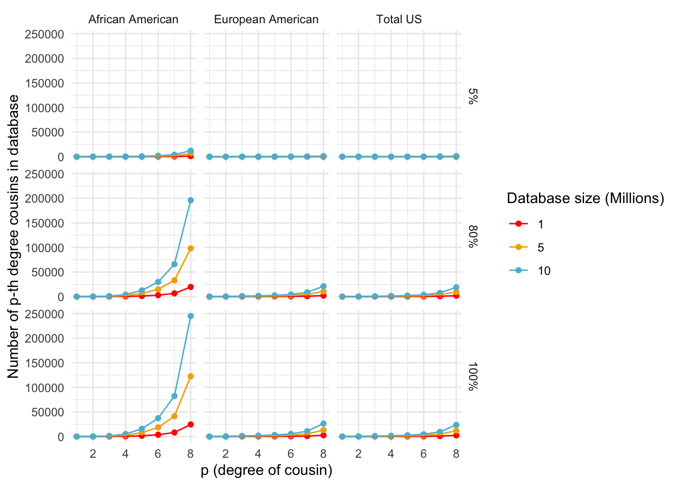
Probability of a genetically detectable cousin
Below, we calculate the expected number of shared blocks of genetic material between cousins of varying degrees of relatedness. This is important because the probability of detecting genetic material that is shared between two individuals decreases as the degree of relatedness between them decreases. The code uses a Poisson distribution assumption to estimate the probability of two cousins sharing at least one, two, or three blocks of genetic material, based on the expected number of shared blocks of genetic material calculated from previous research.
# The variable 'meiosis' represents the number of meiosis events between cousins, where 'p' is the degree of relatedness (i.e. p = 1 for first cousins, p = 2 for second cousins, etc.)
meiosis <- p + 1

## Expected number of blocks shared between cousins
# 'E.num.blocks' is the expected number of blocks of shared genetic material between cousins based on the degree of relatedness and the number of meiosis events between them. This value is calculated based on previous research and is not calculated in this code.
E.num.blocks <- 2 * (33.8 * (2 * meiosis) + 22) / (2^(2 * meiosis - 1))

## Use Poisson assumption
# 'Prob.genetic' is the probability of two cousins sharing at least one block of genetic material based on the expected number of shared blocks calculated in the previous step. The calculation uses a Poisson distribution assumption.
Prob.genetic <- 1 - exp(-E.num.blocks)

# 'prob.g.e.2.blocks' is the probability of two cousins sharing at least two blocks of genetic material based on the expected number of shared blocks calculated in the previous step. The calculation uses a Poisson distribution assumption.
prob.g.e.2.blocks <- 1 - sapply(E.num.blocks, function(expected.num) {sum(dpois(0:1, expected.num))})

# 'prob.g.e.3.blocks' is the probability of two cousins sharing at least three blocks of genetic material based on the expected number of shared blocks calculated in the previous step. The calculation uses a Poisson distribution assumption.
prob.g.e.3.blocks <- 1 - sapply(E.num.blocks, function(expected.num) {sum(dpois(0:2, expected.num))})
General
## Plot for number of shared blocks with p-th degree cousins
# Set layout of plot
layout(t(1))

# Set color palette for plot
my.cols2<-wes_palette("FantasticFox1")[3:5]

# Create a blank plot with labeled axes
plot(c(1,8),c(0,1),type="n",ylab="Probability p-th cousin \"detectable\"",xlab="p.(degree of cousin)")

# Add points for probability of detecting pth cousin with genomic blocks using colors from my.cols2
points(p,Prob.genetic,col=my.cols2[1],pch=19,type="b",lwd=2)
points(p,prob.g.e.2.blocks,col=my.cols2[2],pch=19,type="b",lwd=2)
points(p,prob.g.e.3.blocks,col=my.cols2[3],pch=19,type="b",lwd=2)

# Add a legend to the plot
legend(x="topright",legend=c("Cousins (w. >0 genomic blocks)","Cousins (w. >1 genomic blocks)","Cousins (w. >2 genomic blocks)"),col=my.cols2[1:3],lty=1)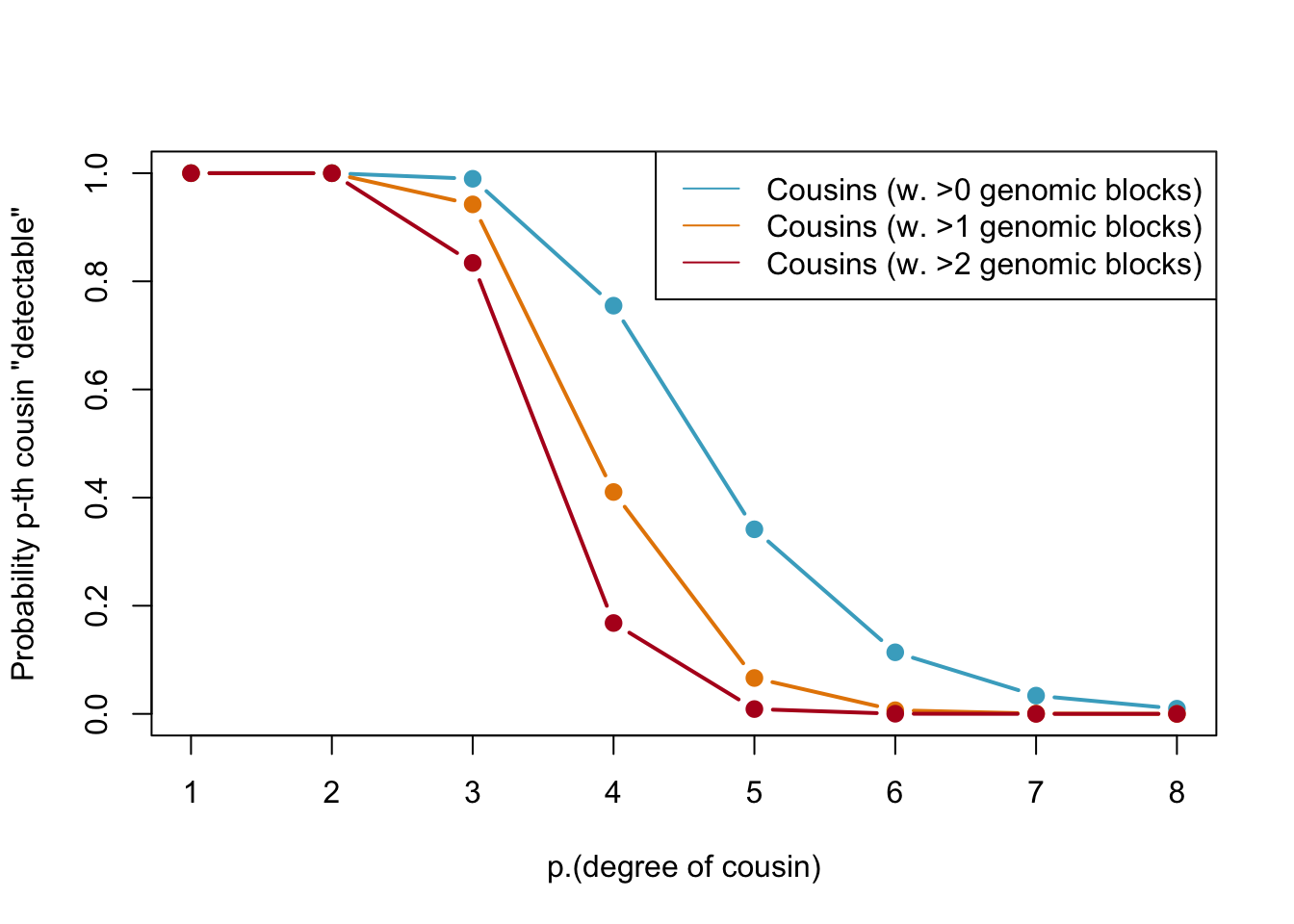
Probabilities of detecting a genetic cousin in a database based on shared genomic blocks. Blue lines represent cousins with at least one genomic block, orange dotted and red lines represent cousins with at least two and three genomic blocks, respectively. The legend specifies the type of cousin being represented by each line.
| Version | Author | Date |
|---|---|---|
| 5f805fe | Tina Lasisi | 2023-03-06 |
Relative to database size
# Function to calculate expected number of p-th degree cousins based on shared genetic blocks
calc_gen_cousins <- function(p, DB.size, N, prob) {
  num.cousins <- 4^(p) * DB.size / (N / 2)
  return(num.cousins * prob)
}

# Function to calculate expected number of p-th degree cousins based on shared genetic blocks for different database fractions
calc_gen_cousins_db_frac <- function(p, DB.sizes, db.frac, N, prob) {
  data <- data.frame(p = integer(), Population = character(), DB.size = double(), Gen_Cousins = double(), Fraction = double())

  for (pop_name in names(N)) {
    for (i in 1:length(db.frac)) {
      for (j in 1:length(DB.sizes)) {
        DB.size <- DB.sizes[j] * db.frac[i]
        num_cousins <- calc_gen_cousins(p, DB.size, N[[pop_name]], prob)
        data <- rbind(data, data.frame(p = p, Population = rep(pop_name, length(p)), DB.size = rep(DB.sizes[j], length(p)), Gen_Cousins = num_cousins, Fraction = rep(db.frac[i], length(p))))
      }
    }
  }

  return(data)
}

# Function to generate ggplot object for expected number of p-th degree cousins based on shared genetic blocks
ggplot_gen_cousins <- function(data, my.cols) {
  plot <- ggplot(data, aes(x = p, y = Gen_Cousins, color = factor(DB.size), group = factor(DB.size))) +
    geom_point() +
    geom_line() +
    scale_color_manual(values = my.cols, name = "Database size (Millions)",
                       labels = format(unique(data$DB.size) / 1e6, nsmall = 0)) +
    labs(x = "p (degree of cousin)", y = "Expected number of genetic p-th cousins in database") +
    theme_minimal() +
    # facet_grid(Fraction ~ Population, labeller = label_parsed)
  facet_grid(Fraction ~ Population, labeller = labeller(Fraction = function(x) sprintf("%.0f%%", as.numeric(x) * 100), Population = c("European American" = "European American", "African American" = "African American", "Total US" = "Total US")))

  return(plot)
}

# Calculate the expected number of p-th degree cousins based on shared genetic blocks for each population and database fraction
gen_cousins_data <- calc_gen_cousins_db_frac(p, DB.sizes, db.frac, populations, prob.g.e.3.blocks)

# Create and display the ggplot object
gen_cousins_plot <- ggplot_gen_cousins(gen_cousins_data, my.cols)
print(gen_cousins_plot)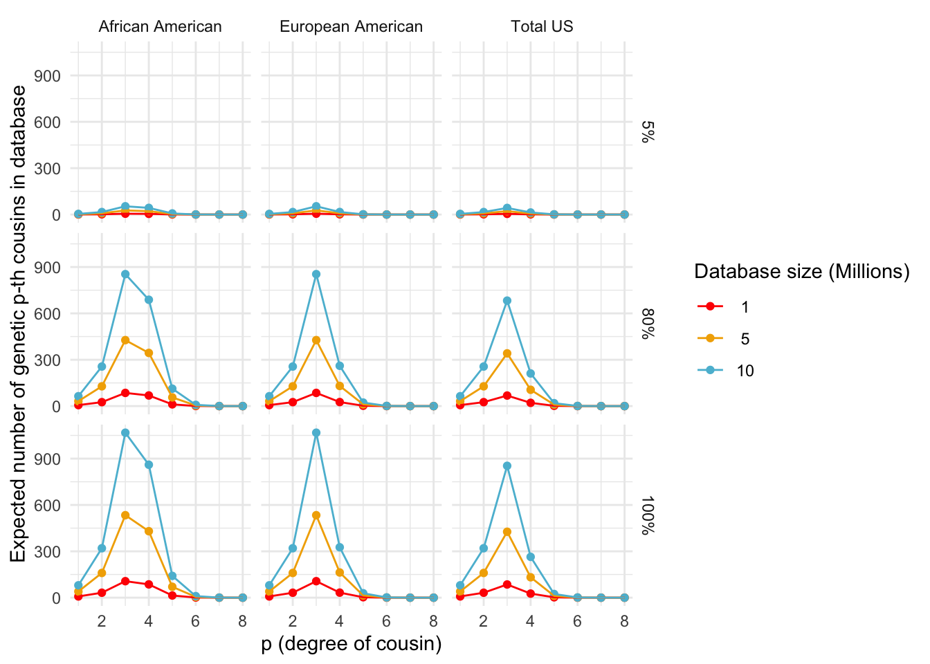
sessionInfo()R version 4.2.2 (2022-10-31)
Platform: aarch64-apple-darwin20 (64-bit)
Running under: macOS Ventura 13.2.1
Matrix products: default
BLAS: /Library/Frameworks/R.framework/Versions/4.2-arm64/Resources/lib/libRblas.0.dylib
LAPACK: /Library/Frameworks/R.framework/Versions/4.2-arm64/Resources/lib/libRlapack.dylib
locale:
[1] en_US.UTF-8/en_US.UTF-8/en_US.UTF-8/C/en_US.UTF-8/en_US.UTF-8
attached base packages:
[1] stats graphics grDevices utils datasets methods base
other attached packages:
[1] forcats_0.5.2 stringr_1.5.0 dplyr_1.0.10 purrr_0.3.5
[5] readr_2.1.3 tidyr_1.2.1 tibble_3.1.8 ggplot2_3.4.0
[9] tidyverse_1.3.2 wesanderson_0.3.6 workflowr_1.7.0
loaded via a namespace (and not attached):
[1] Rcpp_1.0.9 lubridate_1.9.0 getPass_0.2-2
[4] ps_1.7.2 assertthat_0.2.1 rprojroot_2.0.3
[7] digest_0.6.30 utf8_1.2.2 R6_2.5.1
[10] cellranger_1.1.0 backports_1.4.1 reprex_2.0.2
[13] evaluate_0.18 highr_0.9 httr_1.4.4
[16] pillar_1.8.1 rlang_1.0.6 readxl_1.4.1
[19] googlesheets4_1.0.1 rstudioapi_0.14 whisker_0.4
[22] callr_3.7.3 jquerylib_0.1.4 rmarkdown_2.18
[25] labeling_0.4.2 googledrive_2.0.0 munsell_0.5.0
[28] broom_1.0.1 modelr_0.1.10 compiler_4.2.2
[31] httpuv_1.6.6 xfun_0.35 pkgconfig_2.0.3
[34] htmltools_0.5.3 tidyselect_1.2.0 fansi_1.0.3
[37] crayon_1.5.2 withr_2.5.0 tzdb_0.3.0
[40] dbplyr_2.2.1 later_1.3.0 grid_4.2.2
[43] jsonlite_1.8.3 gtable_0.3.1 lifecycle_1.0.3
[46] DBI_1.1.3 git2r_0.30.1 magrittr_2.0.3
[49] scales_1.2.1 cli_3.4.1 stringi_1.7.8
[52] cachem_1.0.6 farver_2.1.1 fs_1.5.2
[55] promises_1.2.0.1 xml2_1.3.3 bslib_0.4.1
[58] ellipsis_0.3.2 generics_0.1.3 vctrs_0.5.1
[61] tools_4.2.2 glue_1.6.2 hms_1.1.2
[64] processx_3.8.0 fastmap_1.1.0 yaml_2.3.6
[67] timechange_0.1.1 colorspace_2.0-3 gargle_1.2.1
[70] rvest_1.0.3 knitr_1.41 haven_2.5.1
[73] sass_0.4.4