About
Last updated: 2024-07-19
Checks: 7 0
Knit directory: KODAMA-Analysis/
This reproducible R Markdown analysis was created with workflowr (version 1.7.1). The Checks tab describes the reproducibility checks that were applied when the results were created. The Past versions tab lists the development history.
Great! Since the R Markdown file has been committed to the Git repository, you know the exact version of the code that produced these results.
Great job! The global environment was empty. Objects defined in the global environment can affect the analysis in your R Markdown file in unknown ways. For reproduciblity it’s best to always run the code in an empty environment.
The command set.seed(20240618) was run prior to running
the code in the R Markdown file. Setting a seed ensures that any results
that rely on randomness, e.g. subsampling or permutations, are
reproducible.
Great job! Recording the operating system, R version, and package versions is critical for reproducibility.
Nice! There were no cached chunks for this analysis, so you can be confident that you successfully produced the results during this run.
Great job! Using relative paths to the files within your workflowr project makes it easier to run your code on other machines.
Great! You are using Git for version control. Tracking code development and connecting the code version to the results is critical for reproducibility.
The results in this page were generated with repository version 3f7aad6. See the Past versions tab to see a history of the changes made to the R Markdown and HTML files.
Note that you need to be careful to ensure that all relevant files for
the analysis have been committed to Git prior to generating the results
(you can use wflow_publish or
wflow_git_commit). workflowr only checks the R Markdown
file, but you know if there are other scripts or data files that it
depends on. Below is the status of the Git repository when the results
were generated:
Unstaged changes:
    Deleted:    analysis/figure/DLPFC-12.Rmd/unnamed-chunk-10-1.png
    Modified:   analysis/index.Rmd
Note that any generated files, e.g. HTML, png, CSS, etc., are not included in this status report because it is ok for generated content to have uncommitted changes.
These are the previous versions of the repository in which changes were
made to the R Markdown (analysis/Giotto.Rmd) and HTML
(docs/Giotto.html) files. If you’ve configured a remote Git
repository (see ?wflow_git_remote), click on the hyperlinks
in the table below to view the files as they were in that past version.
| File | Version | Author | Date | Message |
|---|---|---|---|---|
| Rmd | 3f7aad6 | Stefano Cacciatore | 2024-07-19 | Start my new project |
| Rmd | e7be557 | GitHub | 2024-07-16 | Update Giotto.Rmd |
| html | 40f0fda | GitHub | 2024-07-16 | Update Giotto.html |
| Rmd | b662e13 | GitHub | 2024-07-16 | Update Giotto.Rmd |
| html | 7be8f59 | tkcaccia | 2024-07-15 | updates |
| Rmd | f8ca54a | tkcaccia | 2024-07-14 | update |
| html | f8ca54a | tkcaccia | 2024-07-14 | update |
| Rmd | 89a11c1 | GitHub | 2024-07-08 | Add files via upload |
| html | 2b5aad7 | GitHub | 2024-07-08 | Add files via upload |
Giotto Suite
Introduction to Giotto
Giotto Suite is a collection of open-source software tools, including data structures and methods, for the comprehensive analysis and visualization of spatial multi-omics data at multiple scales and resolutions. More information can be found here.
Dataset Description
The data in this tutorial originates from a Visium Spatial Gene Expression slide of the adult mouse. This dataset is available on the 10X Genomics support site and can be downloaded using the following code.
Library loading
library(KODAMA)
library(KODAMAextra)
library(Giotto)
Dataset loading
instrs = createGiottoInstructions(save_dir = '../Temporary',
                                  save_plot = FALSE,
                                  show_plot = TRUE,
                                  python_path = NULL)


## directly from visium folder
visium_brain = createGiottoVisiumObject(visium_dir = "../Giotto_Mouse_brain/",
                                        expr_data = 'raw',
                                        png_name = 'tissue_lowres_image.png',
                                        gene_column_index = 2,
                                        instructions = instrs,
                                        verbose = FALSE)


## check metadata
pDataDT(visium_brain)
cell_ID in_tissue array_row array_col
<char> <int> <int> <int>
1: AAACAACGAATAGTTC-1 0 0 16
2: AAACAAGTATCTCCCA-1 1 50 102
3: AAACAATCTACTAGCA-1 1 3 43
4: AAACACCAATAACTGC-1 1 59 19
5: AAACAGAGCGACTCCT-1 1 14 94
---
4988: TTGTTTCACATCCAGG-1 1 58 42
4989: TTGTTTCATTAGTCTA-1 1 60 30
4990: TTGTTTCCATACAACT-1 1 45 27
4991: TTGTTTGTATTACACG-1 0 73 41
4992: TTGTTTGTGTAAATTC-1 1 7 51## show plot
spatPlot2D(gobject = visium_brain, cell_color = 'in_tissue', point_size = 2,
cell_color_code = c('0' = 'lightgrey', '1' = 'blue'))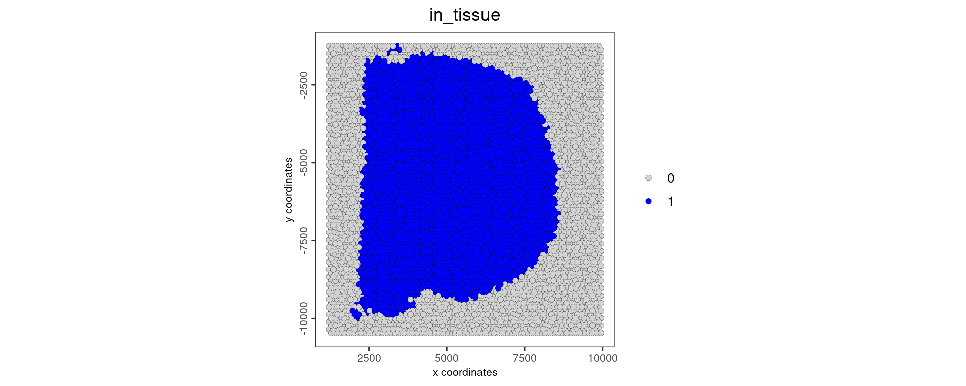 ###Loading and Preparing Data Create Giotto Visium Object
# Provide path to Visium data folder
data_path <- '../Giotto_Mouse_brain/'

# Create Giotto Visium object
visium_brain <- createGiottoVisiumObject(visium_dir = data_path,
                                         expr_data = 'raw',
                                         png_name = 'tissue_lowres_image.png',
                                         gene_column_index = 2,
                                         instructions = instrs)
Preprocessing
## subset on spots that were covered by tissue
metadata = pDataDT(visium_brain)
in_tissue_barcodes = metadata[in_tissue == 1]$cell_ID
visium_brain = subsetGiotto(visium_brain, cell_ids = in_tissue_barcodes)

## filter
visium_brain <- filterGiotto(gobject = visium_brain,
                             expression_threshold = 1,
                             feat_det_in_min_cells = 50,
                             min_det_feats_per_cell = 1000,
                             expression_values = c('raw'),
                             verbose = FALSE)
Normalization and feature reduction
## normalize
visium_brain <- normalizeGiotto(gobject = visium_brain, scalefactor = 6000, verbose = FALSE)

## add gene & cell statistics
visium_brain <- addStatistics(gobject = visium_brain)


visium_brain <- calculateHVF(gobject = visium_brain)


gene_metadata = fDataDT(visium_brain)
featgenes = gene_metadata[hvf == 'yes' & perc_cells > 3 & mean_expr_det > 0.4]$feat_ID

## run PCA on expression values (default)
visium_brain <- runPCA(gobject = visium_brain, feats_to_use = featgenes)
KODAMA analysis
visium_brain=RunKODAMAmatrix(visium_brain, f.par.pls = 50,FUN="PLS",n.cores=4)socket cluster with 4 nodes on host 'localhost'
================================================================================[1] "Finished parallel computation"
[1] "Calculation of dissimilarity matrix..."
================================================================================visium_brain=RunKODAMAvisualization(visium_brain,method="UMAP")Clustering and visualization
visium_brain <- createNearestNetwork(gobject = visium_brain,dim_reduction_to_use = "KODAMA", dim_reduction_name="KODAMA",dimensions_to_use = 1:2, k = 15)

## Leiden clustering
visium_brain <- doLeidenCluster(gobject = visium_brain, resolution = 0.5, n_iterations = 1000,network_name = "sNN.KODAMA")

dimPlot2D(gobject = visium_brain, dim_reduction_to_use ="KODAMA", dim_reduction_name="KODAMA",cell_color = 'leiden_clus',point_size = 2)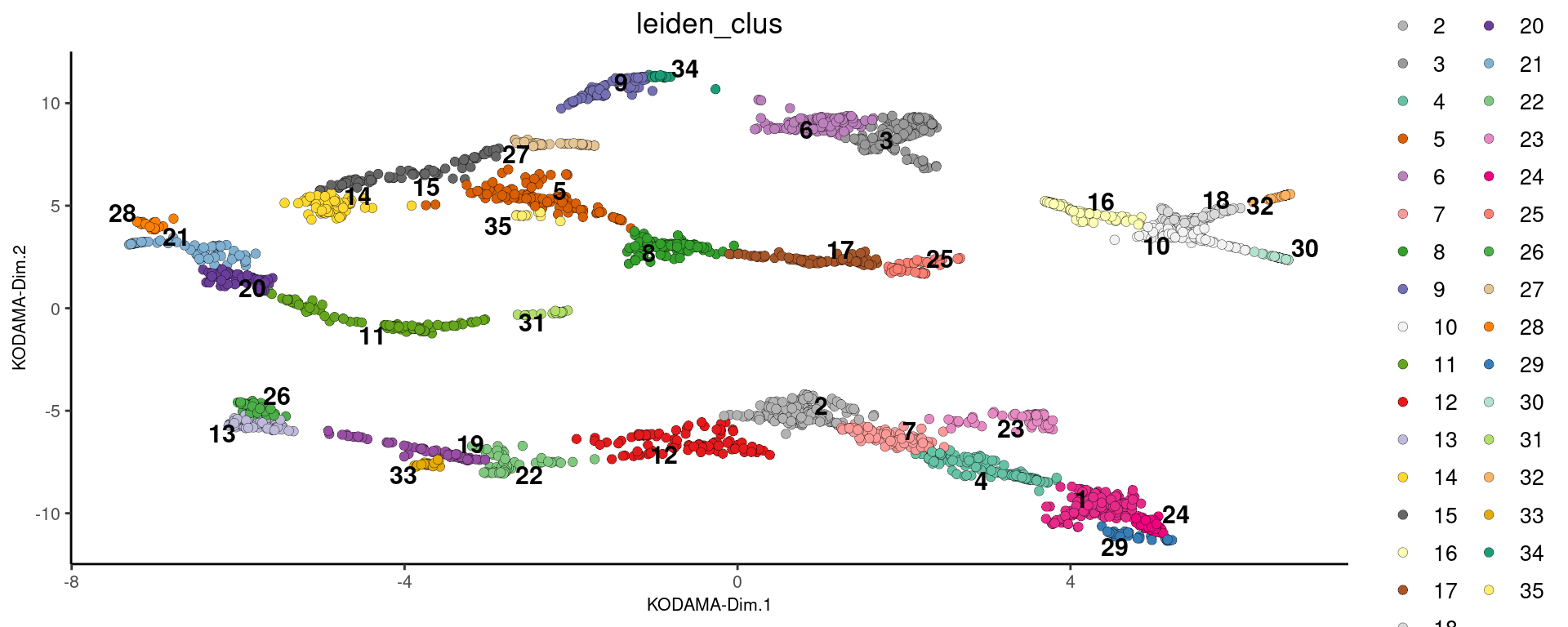
| Version | Author | Date |
|---|---|---|
| 911c63e | GitHub | 2024-07-16 |
spatPlot2D(gobject = visium_brain,cell_color = 'leiden_clus',point_size = 2.5)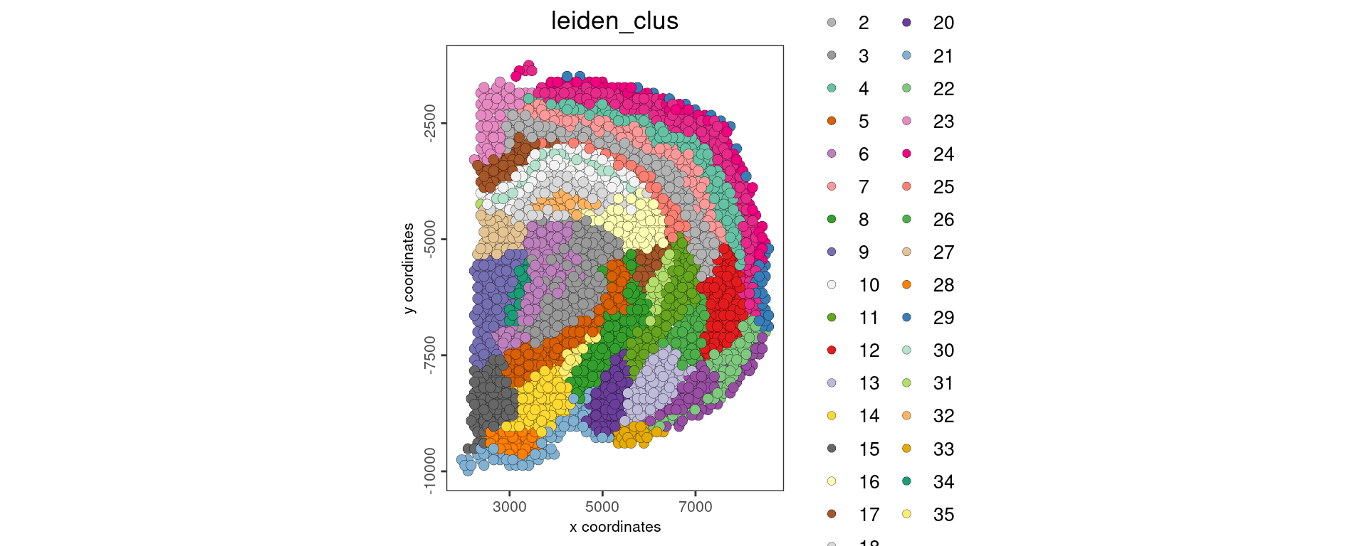
sessionInfo()R version 4.4.1 (2024-06-14)
Platform: x86_64-pc-linux-gnu
Running under: Ubuntu 20.04.6 LTS
Matrix products: default
BLAS: /usr/lib/x86_64-linux-gnu/blas/libblas.so.3.9.0
LAPACK: /usr/lib/x86_64-linux-gnu/lapack/liblapack.so.3.9.0
locale:
[1] LC_CTYPE=en_US.UTF-8 LC_NUMERIC=C
[3] LC_TIME=en_US.UTF-8 LC_COLLATE=en_US.UTF-8
[5] LC_MONETARY=en_US.UTF-8 LC_MESSAGES=en_US.UTF-8
[7] LC_PAPER=en_US.UTF-8 LC_NAME=C
[9] LC_ADDRESS=C LC_TELEPHONE=C
[11] LC_MEASUREMENT=en_US.UTF-8 LC_IDENTIFICATION=C
time zone: Etc/UTC
tzcode source: system (glibc)
attached base packages:
[1] parallel stats graphics grDevices utils datasets methods
[8] base
other attached packages:
[1] Giotto_4.0.8 GiottoClass_0.3.1 KODAMAextra_1.0 e1071_1.7-14
[5] doParallel_1.0.17 iterators_1.0.14 foreach_1.5.2 KODAMA_3.1
[9] umap_0.2.10.0 Rtsne_0.17 minerva_1.5.10 workflowr_1.7.1
loaded via a namespace (and not attached):
[1] RColorBrewer_1.1-3 rstudioapi_0.16.0
[3] jsonlite_1.8.8 magrittr_2.0.3
[5] magick_2.8.4 farver_2.1.2
[7] rmarkdown_2.27 fs_1.6.4
[9] zlibbioc_1.50.0 vctrs_0.6.5
[11] GiottoUtils_0.1.9 askpass_1.2.0
[13] terra_1.7-78 htmltools_0.5.8.1
[15] S4Arrays_1.4.1 SparseArray_1.4.8
[17] parallelly_1.37.1 sass_0.4.9
[19] bslib_0.7.0 htmlwidgets_1.6.4
[21] plyr_1.8.9 plotly_4.10.4
[23] cachem_1.1.0 whisker_0.4.1
[25] igraph_2.0.3 lifecycle_1.0.4
[27] pkgconfig_2.0.3 rsvd_1.0.5
[29] Matrix_1.7-0 R6_2.5.1
[31] fastmap_1.2.0 future_1.33.2
[33] GenomeInfoDbData_1.2.12 MatrixGenerics_1.16.0
[35] digest_0.6.36 colorspace_2.1-0
[37] S4Vectors_0.42.1 ps_1.7.7
[39] rprojroot_2.0.4 irlba_2.3.5.1
[41] RSpectra_0.16-1 GenomicRanges_1.56.1
[43] beachmat_2.20.0 labeling_0.4.3
[45] fansi_1.0.6 httr_1.4.7
[47] abind_1.4-5 compiler_4.4.1
[49] proxy_0.4-27 withr_3.0.0
[51] backports_1.5.0 BiocParallel_1.38.0
[53] highr_0.11 R.utils_2.12.3
[55] openssl_2.2.0 rappdirs_0.3.3
[57] DelayedArray_0.30.1 rjson_0.2.21
[59] gtools_3.9.5 GiottoVisuals_0.2.3
[61] tools_4.4.1 httpuv_1.6.15
[63] future.apply_1.11.2 R.oo_1.26.0
[65] glue_1.7.0 dbscan_1.2-0
[67] callr_3.7.6 promises_1.3.0
[69] grid_4.4.1 checkmate_2.3.1
[71] getPass_0.2-4 reshape2_1.4.4
[73] snow_0.4-4 generics_0.1.3
[75] gtable_0.3.5 R.methodsS3_1.8.2
[77] class_7.3-22 tidyr_1.3.1
[79] data.table_1.15.4 ScaledMatrix_1.12.0
[81] BiocSingular_1.20.0 sp_2.1-4
[83] utf8_1.2.4 XVector_0.44.0
[85] BiocGenerics_0.50.0 ggrepel_0.9.5
[87] pillar_1.9.0 stringr_1.5.1
[89] later_1.3.2 dplyr_1.1.4
[91] lattice_0.22-6 deldir_2.0-4
[93] tidyselect_1.2.1 SingleCellExperiment_1.26.0
[95] knitr_1.48 git2r_0.33.0
[97] IRanges_2.38.1 SummarizedExperiment_1.34.0
[99] scattermore_1.2 stats4_4.4.1
[101] xfun_0.45 Biobase_2.64.0
[103] matrixStats_1.3.0 stringi_1.8.4
[105] UCSC.utils_1.0.0 lazyeval_0.2.2
[107] yaml_2.3.9 evaluate_0.24.0
[109] codetools_0.2-20 tibble_3.2.1
[111] colorRamp2_0.1.0 cli_3.6.3
[113] reticulate_1.38.0 munsell_0.5.1
[115] processx_3.8.4 jquerylib_0.1.4
[117] Rcpp_1.0.12 GenomeInfoDb_1.40.1
[119] doSNOW_1.0.20 globals_0.16.3
[121] png_0.1-8 ggplot2_3.5.1
[123] listenv_0.9.1 SpatialExperiment_1.14.0
[125] viridisLite_0.4.2 scales_1.3.0
[127] purrr_1.0.2 crayon_1.5.3
[129] rlang_1.1.4 cowplot_1.1.3