Ingenuity Pathway Analysis
Ha M. Tran
24/12/2021
Last updated: 2023-01-22
Checks: 7 0
Knit directory: SRB_2022/1_analysis/
This reproducible R Markdown analysis was created with workflowr (version 1.7.0). The Checks tab describes the reproducibility checks that were applied when the results were created. The Past versions tab lists the development history.
Great! Since the R Markdown file has been committed to the Git repository, you know the exact version of the code that produced these results.
Great job! The global environment was empty. Objects defined in the global environment can affect the analysis in your R Markdown file in unknown ways. For reproduciblity it’s best to always run the code in an empty environment.
The command set.seed(12345) was run prior to running the
code in the R Markdown file. Setting a seed ensures that any results
that rely on randomness, e.g. subsampling or permutations, are
reproducible.
Great job! Recording the operating system, R version, and package versions is critical for reproducibility.
Nice! There were no cached chunks for this analysis, so you can be confident that you successfully produced the results during this run.
Great job! Using relative paths to the files within your workflowr project makes it easier to run your code on other machines.
Great! You are using Git for version control. Tracking code development and connecting the code version to the results is critical for reproducibility.
The results in this page were generated with repository version eb10bef. See the Past versions tab to see a history of the changes made to the R Markdown and HTML files.
Note that you need to be careful to ensure that all relevant files for
the analysis have been committed to Git prior to generating the results
(you can use wflow_publish or
wflow_git_commit). workflowr only checks the R Markdown
file, but you know if there are other scripts or data files that it
depends on. Below is the status of the Git repository when the results
were generated:
Ignored files:
    Ignored:    .Rhistory
    Ignored:    .Rproj.user/

Untracked files:
    Untracked:  .gitignore

Unstaged changes:
    Deleted:    1_analysis/mmu04060.pv.png
    Deleted:    1_analysis/mmu04151.pv.png
    Deleted:    1_analysis/mmu04270.pv.png
    Deleted:    1_analysis/mmu04510.pv.png
    Deleted:    1_analysis/mmu04640.pv.png
    Deleted:    1_analysis/mmu04670.pv.png
    Modified:   2_plots/de/ma_1.05.png
    Modified:   2_plots/de/ma_1.1.png
    Modified:   2_plots/de/ma_1.5.png
    Modified:   2_plots/de/vol_1.05.png
    Modified:   2_plots/de/vol_1.1.png
    Modified:   2_plots/de/vol_1.5.png
    Modified:   2_plots/kegg/heat_1.05_Cytokine-cytokine receptor interaction.svg
    Modified:   2_plots/kegg/heat_1.05_Focal adhesion.svg
    Modified:   2_plots/kegg/heat_1.05_Hematopoietic cell lineage.svg
    Modified:   2_plots/kegg/heat_1.05_Leukocyte transendothelial migration.svg
    Modified:   2_plots/kegg/heat_1.05_PI3K-Akt signaling pathway.svg
    Modified:   2_plots/kegg/heat_1.05_Vascular smooth muscle contraction.svg
    Modified:   2_plots/kegg/heat_1.1_Cytokine-cytokine receptor interaction.svg
    Modified:   2_plots/kegg/heat_1.1_Focal adhesion.svg
    Modified:   2_plots/kegg/heat_1.1_Hematopoietic cell lineage.svg
    Modified:   2_plots/kegg/heat_1.1_Leukocyte transendothelial migration.svg
    Modified:   2_plots/kegg/heat_1.1_PI3K-Akt signaling pathway.svg
    Modified:   2_plots/kegg/heat_1.1_Vascular smooth muscle contraction.svg
    Modified:   2_plots/kegg/heat_1.5_Cytokine-cytokine receptor interaction.svg
    Modified:   2_plots/kegg/heat_1.5_Focal adhesion.svg
    Modified:   2_plots/kegg/heat_1.5_Hematopoietic cell lineage.svg
    Modified:   2_plots/kegg/heat_1.5_Leukocyte transendothelial migration.svg
    Modified:   2_plots/kegg/heat_1.5_PI3K-Akt signaling pathway.svg
    Modified:   2_plots/kegg/heat_1.5_Vascular smooth muscle contraction.svg
    Modified:   3_output/enrichGO_sig.xlsx
    Modified:   3_output/enrichKEGG_all.xlsx
    Modified:   3_output/enrichKEGG_sig.xlsx
    Modified:   3_output/lmTreat_all.xlsx
    Modified:   3_output/lmTreat_fc1.5_voom2_all_fdr.xlsx
    Modified:   3_output/lmTreat_sig.xlsx
    Modified:   3_output/reactome_all.xlsx
    Modified:   3_output/reactome_sig.xlsx
    Modified:   README.md
    Deleted:    test plz delete me.Rmd
    Deleted:    test-plz-delete-me.html
Note that any generated files, e.g. HTML, png, CSS, etc., are not included in this status report because it is ok for generated content to have uncommitted changes.
These are the previous versions of the repository in which changes were
made to the R Markdown (1_analysis/extraFigures.Rmd) and
HTML (docs/extraFigures.html) files. If you’ve configured a
remote Git repository (see ?wflow_git_remote), click on the
hyperlinks in the table below to view the files as they were in that
past version.
| File | Version | Author | Date | Message |
|---|---|---|---|---|
| Rmd | eb10bef | Ha Manh Tran | 2023-01-22 | workflowr::wflow_publish(here::here("1_analysis/*.Rmd")) |
| Rmd | 8c9178d | tranmanhha135 | 2023-01-21 | added png |
| html | 8c9178d | tranmanhha135 | 2023-01-21 | added png |
| html | d578f46 | Ha Manh Tran | 2023-01-21 | Build site. |
| Rmd | 01a61cb | Ha Manh Tran | 2023-01-21 | workflowr::wflow_publish(here::here("1_analysis/*.Rmd")) |
| Rmd | 159f352 | tranmanhha135 | 2023-01-21 | adding for pathview |
| html | 159f352 | tranmanhha135 | 2023-01-21 | adding for pathview |
| html | 4d51a4e | tranmanhha135 | 2023-01-20 | test png |
| html | 691cf34 | Ha Manh Tran | 2023-01-20 | Build site. |
| Rmd | 3119fad | tranmanhha135 | 2022-11-05 | build website |
| html | 3119fad | tranmanhha135 | 2022-11-05 | build website |
Data Setup
# working with data
library(dplyr)
library(magrittr)
library(readr)
library(tibble)
library(reshape2)
library(tidyverse)

# Visualisation:
library(kableExtra)
library(ggplot2)
library(grid)
library(pander)
library(cowplot)
library(pheatmap)
library(viridis)
library(igraph)
library(ggalluvial)


# Custom ggplot
library(ggplotify)
library(ggbiplot)
library(ggrepel)
theme_set(theme_minimal())
pub <- readRDS(here::here("0_data/RDS_objects/pub.rds"))
palette <- readRDS(here::here("0_data/RDS_objects/palette.rds"))
IPA analysis
Regulated Pathways
pathways <- read_csv(file = here::here("0_data/raw_data/IPA_pathways.csv"), col_names = T) %>% slice(1:14) %>% as.data.frame()
colnames(pathways) <- c("name", "logPval", "pval", "ratio", "zScore", "molecules")

# at the beginnning of a word (after 35 characters), add a newline. shorten the y axis for dot plot
pathways$name <- sub(
  pattern = "(.{1,40})(?:$| )",
  replacement = "\\1\n",
  x = pathways$name
)

# remove the additional newline at the end of the string
pathways$name <- sub(
  pattern = "\n$",
  replacement = "",
  x = pathways$name
)

pathways <- ggplot(data = pathways) +
  geom_point(aes(
    x = ratio,
    y = reorder(name, logPval),
    color = zScore,
    size = logPval)) +
  scale_size(range = c(2, 7)) +
  scale_color_gradient(low = "dodgerblue3", high = "firebrick3", limits=c(0, NA)) +
  ggtitle("Regulated Pathways") +
  xlab(label = "Gene Ratio") +
  ylab(label = "") +
  labs(color = "Z-Score",
       size = expression("-log"[10] * "P-value")) +
  scale_x_continuous(expand = c(0,0.007))
  # theme(axis.text.x = element_text(angle = 90, hjust = 1, vjust = 0.5))

ggsave(filename = "pathways.svg", plot = pathways, path = here::here("2_plots/ipa"), width = 250, height = 166, units = "mm")
pathways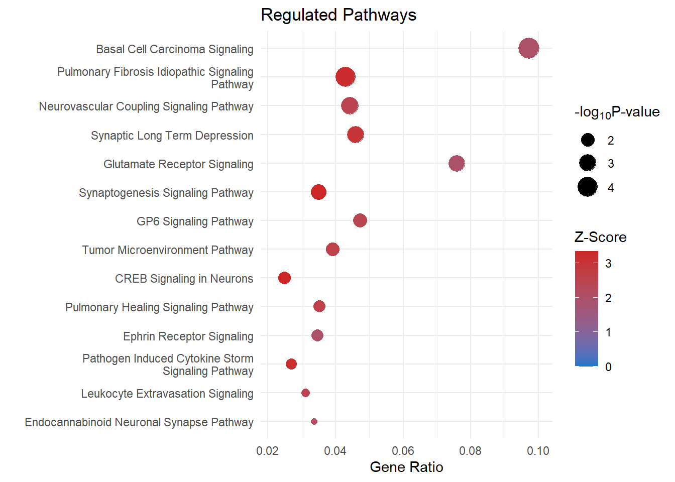
Upstream Regulators
upstream <-
  read_csv(file = here::here("0_data/raw_data/IPA_upstreamRegulators.csv"),
    col_names = T,
    skip = 1) %>% as.data.frame()
# colnames(upstream) <- c("regulator", "logRatio", "molecule", "activationState", "zScore", "flags", "pvalOverlap", "targetMolecule")
# upstream <- column_to_rownames(.data = upstream,var = "Upstream Regulator")
upstream <-
  dplyr::filter(
    .data = upstream,
      `Molecule Type` == "enzyme" |
      `Molecule Type` == "growth factor" |
      `Molecule Type` == "cytokine" |
      `Molecule Type` == "chemical - endogenous mammalian"
  )
heatMatrix <-
  upstream %>% select(c("Upstream Regulator", "Activation z-score")) %>% column_to_rownames("Upstream Regulator")
# %>% pivot_wider(names_from = `Upstream Regulator`, values_from = `Activation z-score`)

# my_palette <- colorRampPalette(c("dodgerblue3", "white", "firebrick3"))(n = 201)
# my_palette <- viridis_pal(option = "viridis")(300)

# df for heatmap annotation of sample group
anno <-
  dplyr::select(.data = upstream, c(`Upstream Regulator`, `Molecule Type`))
# anno %>% column_to_rownames("Upstream Regulator")
anno$`Molecule Type` <- str_to_title(anno$`Molecule Type`)
anno$`Molecule Type` <- as.factor(anno$`Molecule Type`)
anno <- column_to_rownames(.data = anno, var = "Upstream Regulator")

anno_colours <- c("#d7191c", "#fdae61", "#abd9e9", "#2c7bb6")

names(anno_colours) <- levels(anno$`Molecule Type`)

upstream <- pheatmap(
  mat = heatMatrix,
  cluster_rows = F,
  cluster_cols = F,
  show_colnames = F,
  show_rownames = T,
  legend = T,
  annotation_legend = T,
  annotation_row = anno,
  annotation_names_row = F,
  annotation_colors = list("Molecule Type" = anno_colours),
  annotation_names_col = F,
  # annotation = F,
  color = palette,
  fontsize = 8,
  fontsize_col = 6,
  fontsize_number = 5 ,
  fontsize_row = 8,
  legend_breaks = c(seq(-3, 11, by = 1)),
  legend_labels = c(seq(-3, 11, by = 1)),
  border_color = "grey85",
  angle_col = 90,
  gaps_row = c(8, 13, 16)
  ) %>% as.ggplot()
# upstream <- upstream + theme(legend.box.margin = margin(0,0,-150,0))
ggsave(filename = "upstream_2.svg", plot = upstream, path = here::here("2_plots/ipa"), width = 200, height = 133, units = "mm")upstream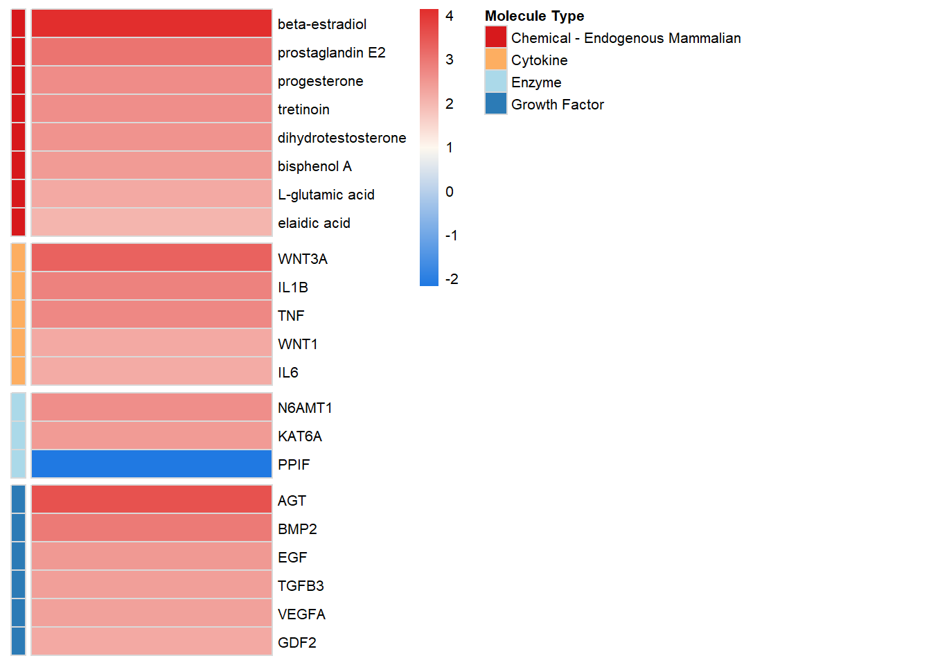
Disease and Function
categories <- c("Cellular Movement", "Cardiovascular System", "Cell-To-Cell Signaling")
tittle <- c("Cellular Movement", "Cardiovascular System Development and Function", "Cell-to-Cell Signaling and Interaction")

disease_function <- read_csv(file = here::here("0_data/raw_data/IPA_diseaseAndFunction.csv"), col_names = T, skip = 1)
disease_function <- drop_na(data = disease_function, "Predicted Activation State")
# disease_function <- dplyr::filter(disease_function, grepl(c(categories), x = disease_function$Categories))

funct=list()
funct_bar=list()
for (i in 1:length(categories)) {
  x <- categories[i] %>% as.character()
  funct[[x]] <-  dplyr::filter(.data = disease_function, grepl(categories[i], x = disease_function$Categories))

  # at the beginnning of a word (after 35 characters), add a newline. shorten the y axis for dot plot
  funct[[x]]$`Diseases or Functions Annotation` <- sub(
    pattern = "(.{1,40})(?:$| )",
    replacement = "\\1\n",
    x = funct[[x]]$`Diseases or Functions Annotation`
    )

  # remove the additional newline at the end of the string
  funct[[x]]$`Diseases or Functions Annotation` <- sub(
    pattern = "\n$",
    replacement = "",
    x = funct[[x]]$`Diseases or Functions Annotation`
    )

  funct_bar[[x]] <- ggplot(data = funct[[x]]) +
    geom_point(aes(
      x = `# Molecules`,
      y = reorder(`Diseases or Functions Annotation`, desc(`p-value`)),
      colour = `Activation z-score`,
      size = -log(`p-value`, 10))) +
  scale_size(range = c(2, 7)) +
  scale_color_gradient(low = "dodgerblue3", high = "firebrick3", limits=c(0, NA)) +
  ggtitle(tittle[i]) +
  xlab(label = "Count") +
  ylab(label = "") +
  labs(colour = "Z-score",
       size = expression("-log"[10] * "P-value")) +
  scale_x_continuous(expand = c(0,5))

ggsave(filename = paste0(x, ".svg"), plot = funct_bar[[i]], path = here::here("2_plots/ipa"), width = 250, height = 166, units = "mm")

}

funct <- do.call(rbind, lapply(funct, as.data.frame)) %>% dplyr::select(-Categories) %>%  rownames_to_column("Categories")
funct$Categories <- gsub(pattern = "\\..*", "", funct$Categories) %>% as.factor()
funct_dot <- ggplot(funct) +
  geom_point(aes(
    x = `# Molecules`,
    y = reorder(`Diseases or Functions Annotation`, desc(`p-value`)),
    colour = `Activation z-score`,
    size = -log(`p-value`, 10),
    shape = `Categories`
  )) +
  facet_grid(vars(`Categories`), scales = "free_y", shrink = T) +
  scale_color_gradient(low = "dodgerblue3", high = "firebrick3", limits=c(0,NA)) +
  xlab(label = "Count") + ylab("") +
  labs(colour = "Z-score",
       size = expression("-log"[10] * "p-value"),
       shape = "Categories") +
  scale_x_continuous(expand = c (0,10)) +
  scale_size(range = c(2,5))
# funct_dot <- funct_dot +
#   theme(
#     panel.background = element_rect(fill='transparent'), #transparent panel bg
#     plot.background = element_rect(fill='transparent', color=NA), #transparent plot bg
#     # panel.grid.major = element_blank(), #remove major gridlines
#     # panel.grid.minor = element_blank(), #remove minor gridlines
#     legend.background = element_rect(fill='transparent'), #transparent legend bg
#     legend.box.background = element_rect(fill='transparent', color=NA) #transparent legend panel
#   )
funct_dot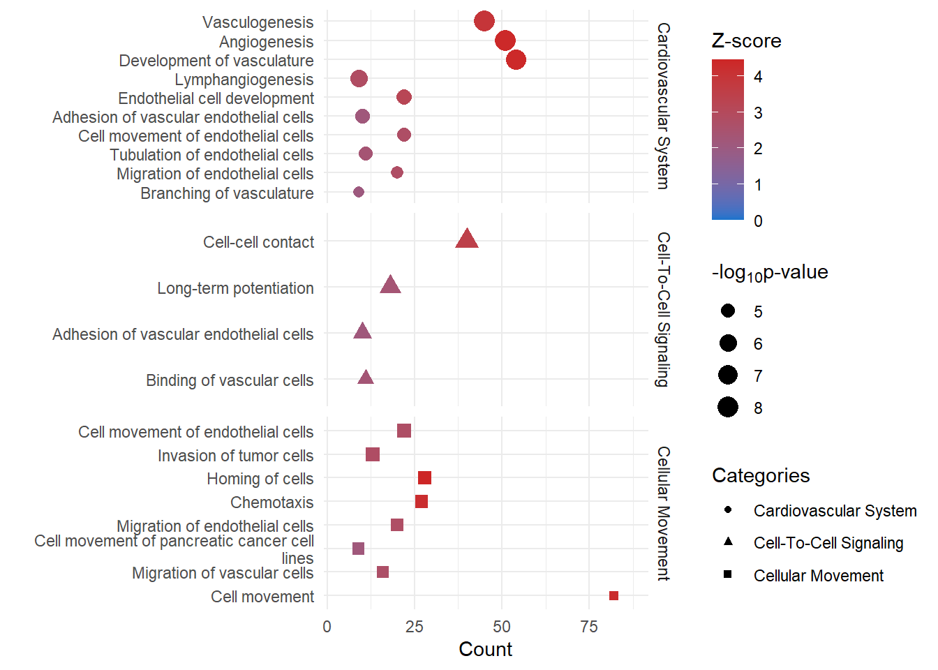
ggsave(filename = "diseaseAndFunction.svg", plot = funct_dot + theme_bw(), path = here::here("2_plots/ipa"), width = 200, height = 300, units = "mm")upstream_filtered <- subset(upstream[c(1,3,19,21,2,18,10,13,11),])
upstream_filtered <- upstream_filtered[order(upstream_filtered$`Molecule Type`),]
test <- separate_rows(data = upstream_filtered, `Target Molecules in Dataset`, sep = ",")
colnames(test)[c(1,8,3)] <- c("name", "molecule", "type")
pathways_filtered <- subset(pathways[c(11,4, 6, 10, 7, 8),])
test1 <- separate_rows(data = pathways_filtered, molecules, sep = ",")
test1[,7] <- "enriched pathways"
colnames(test1)[c(1,6,7)] <- c("name", "molecule", "type" )
funct_filtered <- subset(funct[c(2,3,5,6,7,9,10:21),])
test2 <- separate_rows(data = funct, Molecules, sep = ",")
colnames(test2)[c(2,6,1)] <- c("name", "molecule", "type")
# test_com <- do.call(rbind, lapply(list(test[, c(1, 8, 3)],
# test1[, c(1, 6, 7)]), as.data.frame))
# write.csv(test_com, here::here("C:\\Users/tranm/Desktop/test_com.csv"))
#
# testGraph <- graph.data.frame(test_com, directed = T)
# # testReverse <- as_data_frame(testGraph)
# # E(testGraph)$color <- 'grey'
# # V(testGraph)$color <- 'grey'
# summary(testGraph)
# write_graph(simplify(testGraph), "C:\\Users/tranm/Desktop/testGraph.gml", format = "gml")
# tkplot(testGraph)
merged <- list()
for (i in 1:length(upstream_filtered$`Upstream Regulator`)) {
x <- upstream_filtered$`Upstream Regulator`[i]
for (j in 1:length(funct_filtered$`Diseases or Functions Annotation`)) {
y <- paste0("funct",j)
merged[[x]][[y]] <- length(intersect(unlist(
strsplit(upstream_filtered$`Target Molecules in Dataset`[i], split = ",")
), unlist(strsplit(funct_filtered$Molecules[j], split = ","))))
}
merged[[x]] <- do.call(rbind, lapply(merged[[x]], as.data.frame)) %>% remove_rownames()
merged[[x]][, c( "funct", "funct_cat")] <-
c(funct_filtered$`Diseases or Functions Annotation`,
funct_filtered$Categories %>% as.character()
)
print(i)
}
merged <- do.call(rbind, lapply(merged, as.data.frame)) %>% rownames_to_column("upstream")
merged$upstream <- gsub(pattern = "\\..*", "",merged$upstream) %>% as.factor()
merged$funct_cat <- as.factor(merged$funct_cat)
colnames(merged) <- c("upstream","intersect","funct","funct_cat")
levels(merged$upstream) <- c("beta-estradiol","progesterone","prostaglandin E2","IL1B","IL6","TNF","EGF","VEGFA","BMP2")
####THIS is really weird
# merged$upstream <- gsub(pattern = "protagladin E2",replacement = "prostaglandin E2", merged$upstream)
merged$up_cat <- upstream_filtered$`Molecule Type`[match(merged$upstream, upstream_filtered$`Upstream Regulator`)]
merged$funct <- factor(merged$funct, levels = unique(merged$funct[order(merged$funct_cat)]))
is_alluvia_form(as.data.frame(merged), silent = T)
ggplot(
as.data.frame(merged),
aes(
y = intersect,
# axis1 = up_cat,
axis2 = upstream,
axis3 = funct
# axis4 = funct_cat
)
) +
geom_alluvium(
aes(fill = upstream),
alpha = 0.5,
width = 1 / 250,
curve_type = "quintic"
) +
geom_stratum(fill = "#193e3f",
width = 1 / 35,
color = "#fffaf2") +
# geom_flow() +
geom_text(stat = "stratum", aes(label = after_stat(stratum))) +
scale_x_discrete(
limits =
c(
# "Molecule Type",
"Upstream Regulator",
"Disease and Function"
# "Category"
),
expand = c(.05, .05)
) +
scale_fill_brewer(type = "qual", palette = "Set1") +
theme_void() +
theme(legend.position = "none")
# ylab(" ")
ggsave(filename = "upstream_funct_alluvial.svg",path = here::here("2_plots/ipa/"), width = 450, height = 800, units = "mm")
ggplot(
as.data.frame(merged),
aes(
y = intersect,
axis1 = funct,
axis2 = funct_cat
# axis3 = funct_cat
)
) +
geom_alluvium(aes(fill = funct_cat), alpha = 0.5, width = 1 / 250, curve_type = "quintic") +
geom_stratum(fill = "#193e3f", width = 1 / 35, color = "#fffaf2") +
# geom_flow() +
# geom_text(stat = "stratum", aes(label = after_stat(stratum))) +
scale_x_discrete(
limits = c("Upstream Regulator", "Disease and Function"),
expand = c(.05, .05)
) +
scale_fill_brewer(type = "qual", palette = "Set2") +
theme_void() +
theme(legend.position = "none")
# ylab(" ")
ggsave(filename = "funct_cat_alluvial.svg",path = here::here("2_plots/ipa/"), width = 450, height = 800, units = "mm")
gephi_colours <- colorRampPalette(c("#00c7ff","#ff7045","#8cb900","black"))
ggplot(
as.data.frame(merged),
aes(
y = intersect,
axis1 = up_cat,
axis2 = upstream
)
) +
geom_alluvium(aes(fill = up_cat), alpha = 0.5, width = 1 / 250, curve_type = "quintic") +
geom_stratum(fill = "#193e3f", width = 1 / 35, color = "#fffaf2") +
# geom_flow() +
# geom_text(stat = "stratum", aes(label = after_stat(stratum))) +
scale_x_discrete(
limits = c("Upstream Regulator", "Disease and Function"),
expand = c(.05, .05)
) +
scale_fill_manual(c("#c5da79","#ffb59c","#7fe1f9")) +
theme_void() +
theme(legend.position = "none")
# ylab(" ")
ggsave(filename = "up_cat_alluvial.svg",path = here::here("2_plots/ipa/"), width = 450, height = 800, units = "mm")Network plot

DE genes regulated by predicted upstream regulators and pathways
Alluvial plot

Proportion of DE genes regulated by predicted upstream regulators & functional terms
sessionInfo()R version 4.2.1 (2022-06-23 ucrt)
Platform: x86_64-w64-mingw32/x64 (64-bit)
Running under: Windows 10 x64 (build 19045)
Matrix products: default
locale:
[1] LC_COLLATE=English_Australia.utf8 LC_CTYPE=English_Australia.utf8
[3] LC_MONETARY=English_Australia.utf8 LC_NUMERIC=C
[5] LC_TIME=English_Australia.utf8
attached base packages:
[1] grid stats graphics grDevices utils datasets methods
[8] base
other attached packages:
[1] ggrepel_0.9.1 ggbiplot_0.55 scales_1.2.1 plyr_1.8.7
[5] ggplotify_0.1.0 ggalluvial_0.12.3 igraph_1.3.5 viridis_0.6.2
[9] viridisLite_0.4.1 pheatmap_1.0.12 cowplot_1.1.1 pander_0.6.5
[13] kableExtra_1.3.4 forcats_0.5.2 stringr_1.4.1 purrr_0.3.5
[17] tidyr_1.2.1 ggplot2_3.3.6 tidyverse_1.3.2 reshape2_1.4.4
[21] tibble_3.1.8 readr_2.1.3 magrittr_2.0.3 dplyr_1.0.10
loaded via a namespace (and not attached):
[1] fs_1.5.2 bit64_4.0.5 lubridate_1.8.0
[4] webshot_0.5.4 RColorBrewer_1.1-3 httr_1.4.4
[7] rprojroot_2.0.3 tools_4.2.1 backports_1.4.1
[10] bslib_0.4.0 utf8_1.2.2 R6_2.5.1
[13] DBI_1.1.3 colorspace_2.0-3 withr_2.5.0
[16] tidyselect_1.2.0 gridExtra_2.3 bit_4.0.4
[19] compiler_4.2.1 git2r_0.30.1 textshaping_0.3.6
[22] cli_3.4.1 rvest_1.0.3 xml2_1.3.3
[25] labeling_0.4.2 sass_0.4.2 yulab.utils_0.0.5
[28] systemfonts_1.0.4 digest_0.6.29 rmarkdown_2.17
[31] svglite_2.1.0 pkgconfig_2.0.3 htmltools_0.5.3
[34] highr_0.9 dbplyr_2.2.1 fastmap_1.1.0
[37] rlang_1.0.6 readxl_1.4.1 rstudioapi_0.14
[40] farver_2.1.1 gridGraphics_0.5-1 jquerylib_0.1.4
[43] generics_0.1.3 jsonlite_1.8.2 vroom_1.6.0
[46] googlesheets4_1.0.1 Rcpp_1.0.9 munsell_0.5.0
[49] fansi_1.0.3 lifecycle_1.0.3 stringi_1.7.8
[52] whisker_0.4 yaml_2.3.5 parallel_4.2.1
[55] promises_1.2.0.1 crayon_1.5.2 haven_2.5.1
[58] hms_1.1.2 knitr_1.40 pillar_1.8.1
[61] reprex_2.0.2 glue_1.6.2 evaluate_0.17
[64] modelr_0.1.9 vctrs_0.4.2 tzdb_0.3.0
[67] httpuv_1.6.6 cellranger_1.1.0 gtable_0.3.1
[70] assertthat_0.2.1 cachem_1.0.6 xfun_0.33
[73] broom_1.0.1 later_1.3.0 ragg_1.2.3
[76] googledrive_2.0.0 gargle_1.2.1 workflowr_1.7.0
[79] ellipsis_0.3.2 here_1.0.1