Map Creation
Troy Rowan
2020-07-09
Last updated: 2020-09-03
Checks: 7 0
Knit directory: local_adaptation_sequence/
This reproducible R Markdown analysis was created with workflowr (version 1.6.2). The Checks tab describes the reproducibility checks that were applied when the results were created. The Past versions tab lists the development history.
Great! Since the R Markdown file has been committed to the Git repository, you know the exact version of the code that produced these results.
Great job! The global environment was empty. Objects defined in the global environment can affect the analysis in your R Markdown file in unknown ways. For reproduciblity it’s best to always run the code in an empty environment.
The command set.seed(20200709) was run prior to running the code in the R Markdown file. Setting a seed ensures that any results that rely on randomness, e.g. subsampling or permutations, are reproducible.
Great job! Recording the operating system, R version, and package versions is critical for reproducibility.
Nice! There were no cached chunks for this analysis, so you can be confident that you successfully produced the results during this run.
Great job! Using relative paths to the files within your workflowr project makes it easier to run your code on other machines.
Great! You are using Git for version control. Tracking code development and connecting the code version to the results is critical for reproducibility.
The results in this page were generated with repository version df75bfc. See the Past versions tab to see a history of the changes made to the R Markdown and HTML files.
Note that you need to be careful to ensure that all relevant files for the analysis have been committed to Git prior to generating the results (you can use wflow_publish or wflow_git_commit). workflowr only checks the R Markdown file, but you know if there are other scripts or data files that it depends on. Below is the status of the Git repository when the results were generated:
Ignored files:
    Ignored:    .Rhistory
    Ignored:    .Rproj.user/
    Ignored:    data/PRISM_ppt_30yr_normal_4kmM2_annual_asc.asc
    Ignored:    data/animal_table.rds
    Ignored:    desktop.ini
    Ignored:    output/desktop.ini
    Ignored:    output/k10.allvars.seed2.rds
    Ignored:    output/k9.allvars.seed1.rds
    Ignored:    output/k9.allvars.seed2.rds
    Ignored:    output/k9.threevars.seed1.rds
    Ignored:    output/k9.threevars.seed2.rds
    Ignored:    output/kmeans_plotlist.RDS

Untracked files:
    Untracked:  data/200730_ASA_AllGenotypes.csv
    Untracked:  data/200820_sample_sheet.csv
    Untracked:  data/license.txt
    Untracked:  data/mizzou-data-request/
    Untracked:  data/prism_climate_data/
    Untracked:  data/us-zip-code-latitude-and-longitude.csv
    Untracked:  data/uszips.csv
    Untracked:  data/uszips.xlsx
    Untracked:  output/200822_Lab_IDs.csv
    Untracked:  output/zipcode_zones.csv

Unstaged changes:
    Modified:   code/cluster/200822_SIM.cluster.json
    Modified:   code/config/200822_SIM.config.yaml
    Modified:   code/map_functions.R
Note that any generated files, e.g. HTML, png, CSS, etc., are not included in this status report because it is ok for generated content to have uncommitted changes.
These are the previous versions of the repository in which changes were made to the R Markdown (analysis/map_making.Rmd) and HTML (docs/map_making.html) files. If you’ve configured a remote Git repository (see ?wflow_git_remote), click on the hyperlinks in the table below to view the files as they were in that past version.
| File | Version | Author | Date | Message |
|---|---|---|---|---|
| Rmd | df75bfc | Troy Rowan | 2020-09-03 | added 3,4,all K=9 figures for comparison |
| html | a660a62 | Troy Rowan | 2020-08-31 | Build site. |
| Rmd | 222e47b | Troy Rowan | 2020-08-31 | cleaned up tables and removed K=10 from animal locations file |
| html | 4b17e7e | Troy Rowan | 2020-08-31 | Build site. |
| Rmd | 27eb0df | Troy Rowan | 2020-08-31 | Simmental data dump locations |
| html | 231d3ea | Troy Rowan | 2020-07-28 | Build site. |
| Rmd | 31b23af | Troy Rowan | 2020-07-28 | Added environmental variable PCA |
| html | 3b006f8 | Troy Rowan | 2020-07-14 | Build site. |
| Rmd | bb4e504 | Troy Rowan | 2020-07-14 | Added tabs to maps and section on env variable correlations |
| html | 73221c6 | Troy Rowan | 2020-07-10 | Build site. |
| Rmd | ff7fd0f | Troy Rowan | 2020-07-10 | Checking to see if tabs work for maps on website now |
| html | ae01f68 | Troy Rowan | 2020-07-10 | Build site. |
| Rmd | 5dad063 | Troy Rowan | 2020-07-10 | Fixed tabset plotting for kmeans maps |
| html | d64c6ee | Troy Rowan | 2020-07-10 | Build site. |
| Rmd | 897d00b | Troy Rowan | 2020-07-10 | Fixed link |
| html | d2da211 | Troy Rowan | 2020-07-10 | Build site. |
| Rmd | c205415 | Troy Rowan | 2020-07-10 | Extensive reworking to make initial website with maps example |
| Rmd | a2d16f5 | Troy Rowan | 2020-07-09 | Added page for map making and starte exploring k-means approach |
Introduction
This uses k-means clustering and 30-year normal climate variables to divide the United States into distinct ecoregions.
Reading in climate raster files
These originate from the Prism Climate Group’s website in .bil format I was having issues with the rgdal package reading these or any other form, so had to read them and save as RDS files on Workstation (the only place where rgdal installs properly). SCP’d RDS files here, and these read in the individal environment variable rasters.
temp_raster =
  readRDS(
    here::here("data", "prism_climate_data", "temp_raster.RDS"))

precip_raster =
  readRDS(
    here::here("data", "prism_climate_data", "precip_raster.RDS"))

elev_raster =
  readRDS(
    here::here("data", "prism_climate_data", "elev_raster.RDS"))

dewpt_raster =
  readRDS(
    here::here("data", "prism_climate_data", "mean_dwpt_raster.RDS")
  )

min_vap_raster =
  readRDS(
    here::here("data", "prism_climate_data", "min_vpd_raster.RDS"))

max_vap_raster =
  readRDS(
    here::here("data", "prism_climate_data", "max_vpd_raster.RDS"))

min_temp_raster =
  readRDS(
    here::here("data", "prism_climate_data", "min_temp_raster.RDS"))

max_temp_raster =
  readRDS(
    here::here("data", "prism_climate_data", "max_temp_raster.RDS"))
stacked_raster =
stack(
temp_raster,
precip_raster,
elev_raster,
dewpt_raster,
max_temp_raster,
min_temp_raster,
max_vap_raster,
min_vap_raster
)
threevar_stacked_raster =
stack(
temp_raster,
precip_raster,
elev_raster
)
fourvar_stacked_raster =
stack(
temp_raster,
precip_raster,
elev_raster,
min_vap_raster
)Environmental varible correlations
Numerical Correlations for complete environmental data
env_correlations =
  stacked_raster %>%
    as.data.frame() %>%
    rename("Temperature" = "band1.1",
      "Precipitation" = "band1.2",
      "Elevation" = "band1.3",
      "DewPoint" = "band1.4",
      "MaxTemperature" = "band1.5",
      "MinTemperature" = "band1.6",
      "MaxVaporPressure" = "band1.7",
      "MinVaporPressure" = "band1.8") %>%
    na.omit() %>%
    cor()

env_correlations_p_values =
  stacked_raster %>%
    as.data.frame() %>%
    rename("Temperature" = "band1.1",
      "Precipitation" = "band1.2",
      "Elevation" = "band1.3",
      "DewPoint" = "band1.4",
      "MaxTemperature" = "band1.5",
      "MinTemperature" = "band1.6",
      "MaxVaporPressure" = "band1.7",
      "MinVaporPressure" = "band1.8") %>%
    na.omit() %>%
  cor_pmat()

kable(round(env_correlations, 3))| Temperature | Precipitation | Elevation | DewPoint | MaxTemperature | MinTemperature | MaxVaporPressure | MinVaporPressure | |
|---|---|---|---|---|---|---|---|---|
| Temperature | 1.000 | 0.221 | -0.502 | 0.807 | 0.979 | 0.978 | 0.692 | 0.296 |
| Precipitation | 0.221 | 1.000 | -0.490 | 0.593 | 0.080 | 0.356 | -0.398 | -0.486 |
| Elevation | -0.502 | -0.490 | 1.000 | -0.796 | -0.380 | -0.605 | 0.054 | 0.292 |
| DewPoint | 0.807 | 0.593 | -0.796 | 1.000 | 0.701 | 0.880 | 0.163 | -0.262 |
| MaxTemperature | 0.979 | 0.080 | -0.380 | 0.701 | 1.000 | 0.914 | 0.802 | 0.371 |
| MinTemperature | 0.978 | 0.356 | -0.605 | 0.880 | 0.914 | 1.000 | 0.550 | 0.206 |
| MaxVaporPressure | 0.692 | -0.398 | 0.054 | 0.163 | 0.802 | 0.550 | 1.000 | 0.752 |
| MinVaporPressure | 0.296 | -0.486 | 0.292 | -0.262 | 0.371 | 0.206 | 0.752 | 1.000 |
Correlation heat plots
This plot uses heirchical clustering to group variables
ggcorrplot(env_correlations,
           hc.order = TRUE)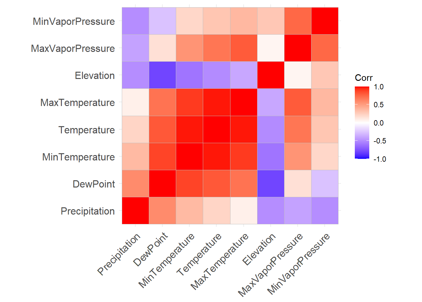
PCA of all PRISM environmental variables
PCA Plot (PC 1 & PC 2)
This shows only loadings of variables (thought that 481,630 was too many points)
fviz_pca_var(env_pca,
             col.var = "contrib", # Color by contributions to the PC
             gradient.cols = c("#00AFBB", "#E7B800", "#FC4E07"),
             repel = TRUE     # Avoid text overlapping
             )+
  ggtitle("Environmental Variable PCA (PC1 & PC2")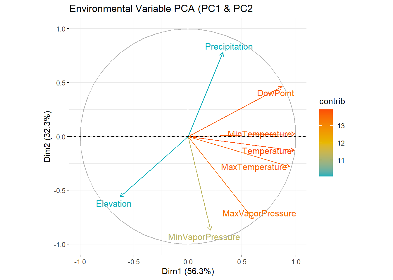
Scree Plot
Vast majority of environmental variance is explained by first two PCs
fviz_eig(env_pca)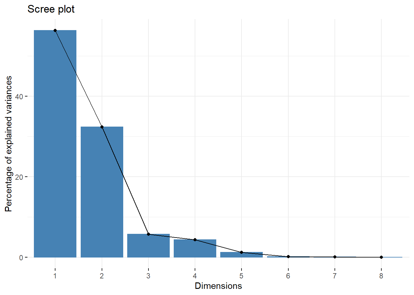
Identifying best K for full- and three-variable datasets
Using fpc::pamk(), K between 3 and 10 This doesn’t run, but appears that based on the fviz_nbclust() function in that the appropriate
It appears that k=2 is optimal by these metrics, but for some reason this step exceeds memory necessary to add to website. While K = 2 may be optimal in a statistical sense, it doesn’t necessarily mean that it’s useful for our analysis (being able to group individuals into subpopulations)
stacked_raster %>%
  as.data.frame() %>%
  na.omit() %>%
  sample_n(20000) %>%
  fviz_nbclust(FUNcluster = kmeans)+
  ggtitle("Full Environmental Data")
  #pamk(krange = 3:20, criterion="multiasw", usepam=FALSE, scaling=TRUE)

threevar_stacked_raster %>%
  as.data.frame() %>%
  na.omit() %>%
  sample_n(20000) %>%
  fviz_nbclust(FUNcluster = kmeans)+
  ggtitle("Three Environmental Variables ")
  #pamk(krange = 3:20, criterion="multiasw", usepam=FALSE, scaling=TRUE)

fourvar_stacked_raster %>%
  as.data.frame() %>%
  na.omit() %>%
  sample_n(20000) %>%
  fviz_nbclust(FUNcluster = kmeans)+
  ggtitle("Three Environmental Variables ") %>%
  #pamk(krange = 3:20, criterion="multiasw", usepam=FALSE, scaling=TRUE)
K-means clustering climate maps
These are the resulting maps from using the full PRISM dataset (all 8 variables) or just three (Temperature, Precipitation, Elevation).
Here, since this is a completely stochastic process, colors don’t have any meaning between K’s or between all data vs. three variables.
I’m particulary intersted in how K=10 breaks out the “Fescue Belt” in both the ALL and Three variable cases.
# plotlist =
#   seq(2,10) %>%
#   purrr::map(
#   ~plot_grid(
#     unsuperClass(stacked_raster,
#                nSamples=2000,
#                nClasses = .x,
#                norm=TRUE,
#                nStarts=5,
#                clusterMap=FALSE) %>%
#     .$map %>%
#     as.data.frame(xy=TRUE) %>%
#     mutate(layer = as.factor(layer)) %>%
#     kmeans_map()+
#       ggtitle(paste("All Variables, k =", .x)),
#     unsuperClass(threevar_stacked_raster,
#                  nSamples=1000,
#                  nClasses = .x,
#                  norm=TRUE,
#                  nStarts=5,
#                  clusterMap=FALSE) %>%
#     .$map %>%
#     as.data.frame(xy=TRUE) %>%
#     mutate(layer = as.factor(layer)) %>%
#     kmeans_map()+
#       ggtitle(paste("Three Variables, k =", .x))
#     )
#   )
#
# saveRDS(plotlist, "../output/kmeans_plotlist.RDS")


plotlist = readRDS(here::here("output", "kmeans_plotlist.RDS"))
#
# for (i in 1:length(plotlist)){
#   cat("### ", i)
#   print(plotlist[[i]])
#   #cat(' \n\n')
# }
K = 2
plotlist[[1]]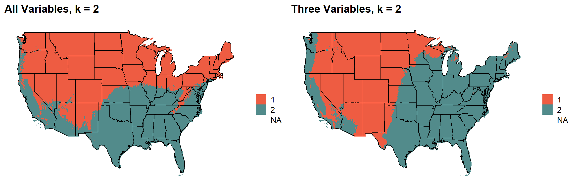
K = 3
plotlist[[2]]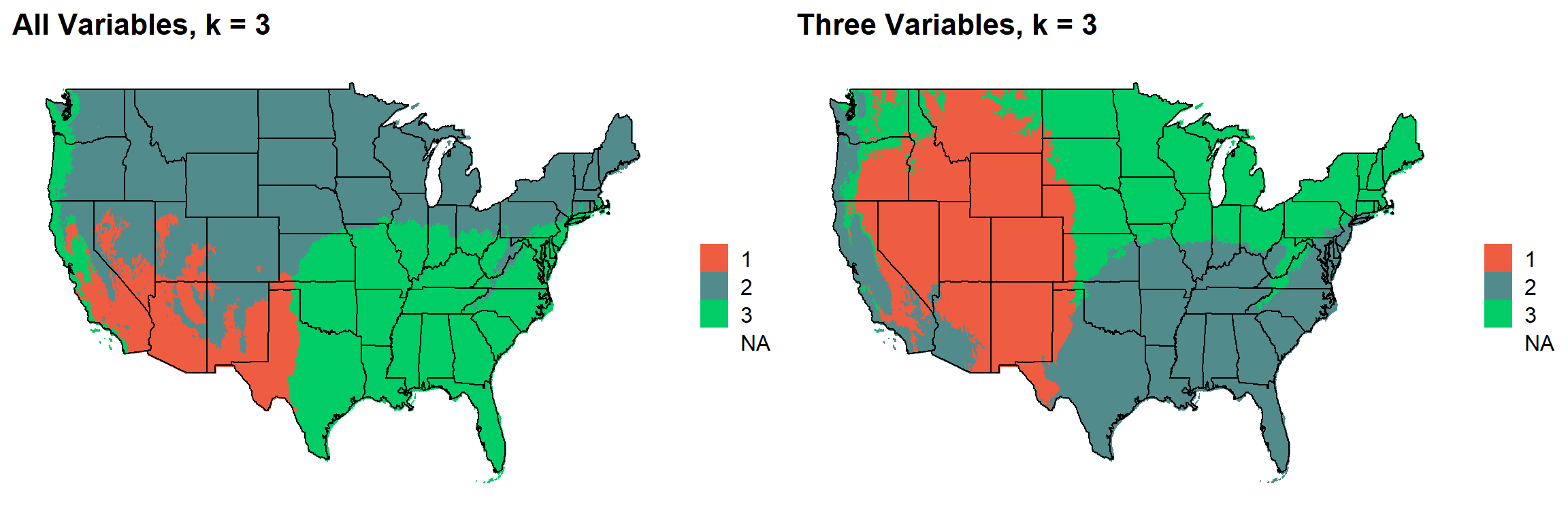
K = 4
plotlist[[3]]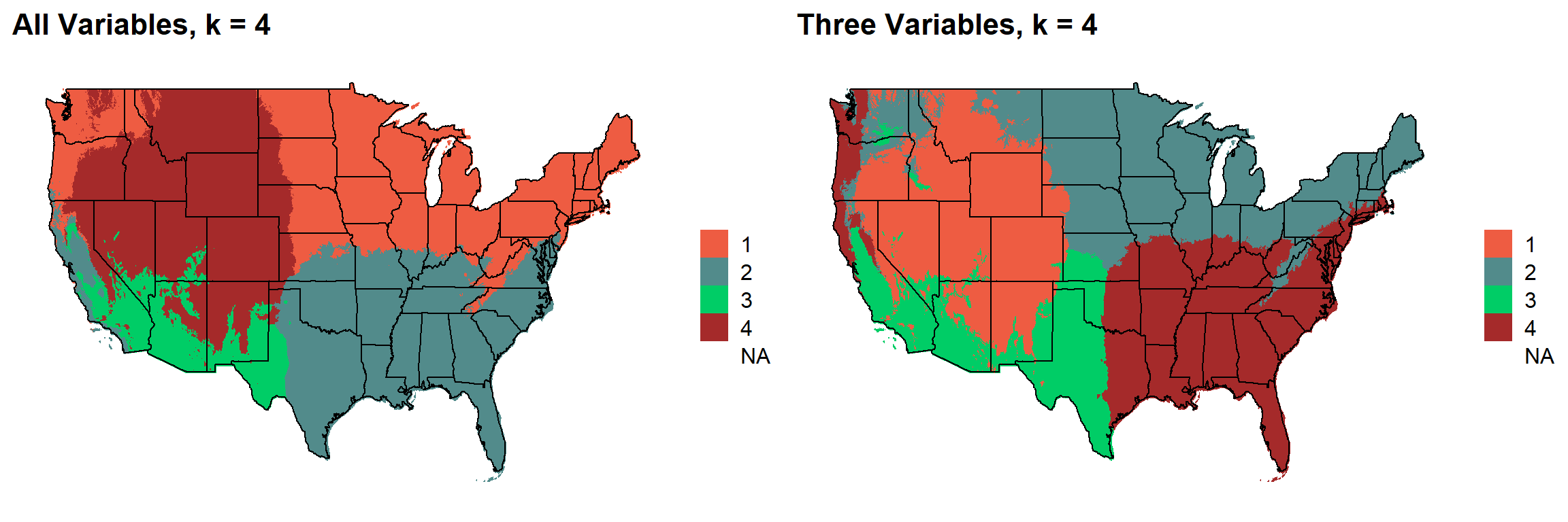
K = 5
plotlist[[4]]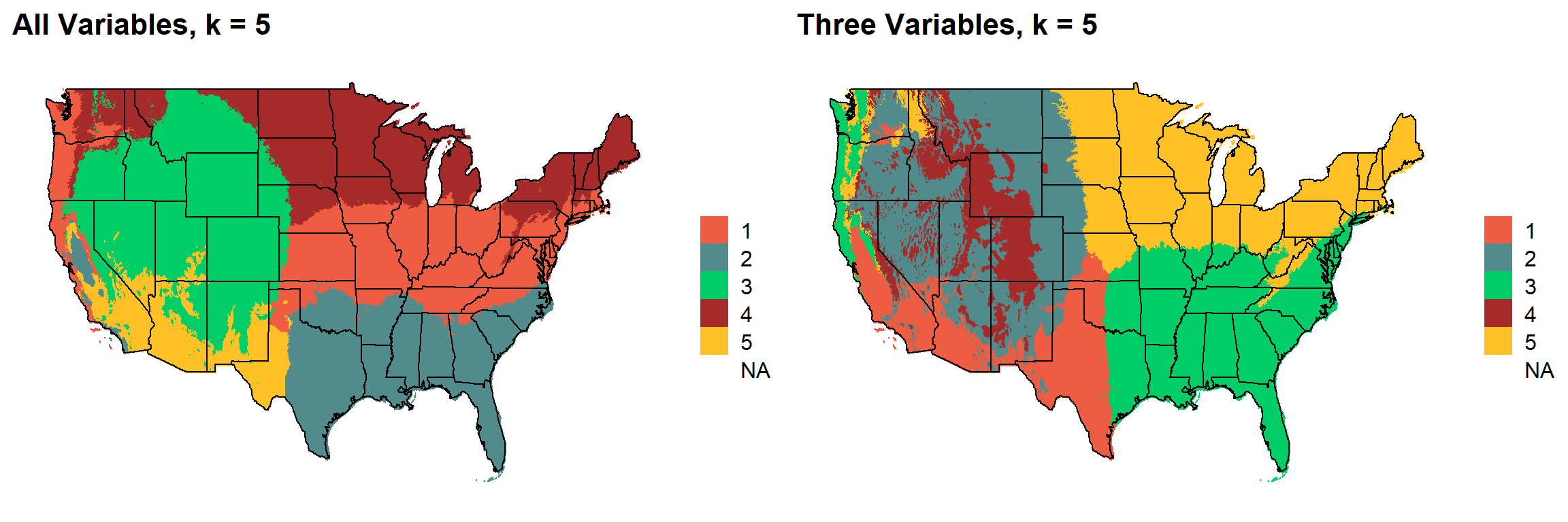
K = 6
plotlist[[5]]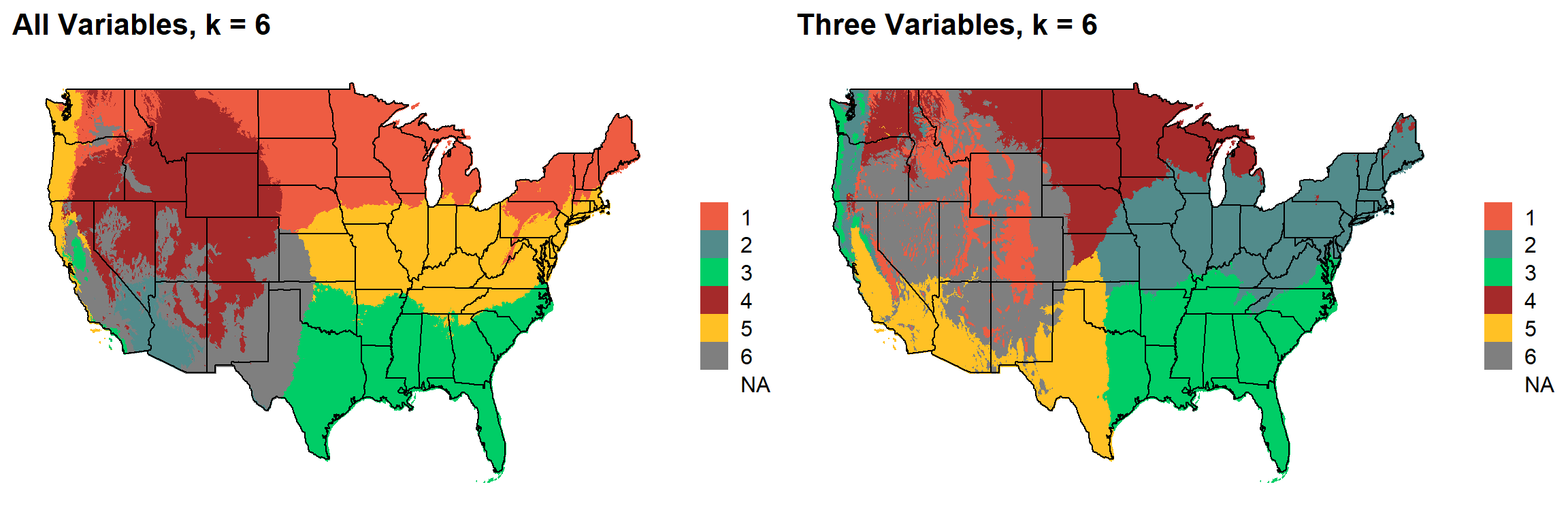
K = 7
plotlist[[6]]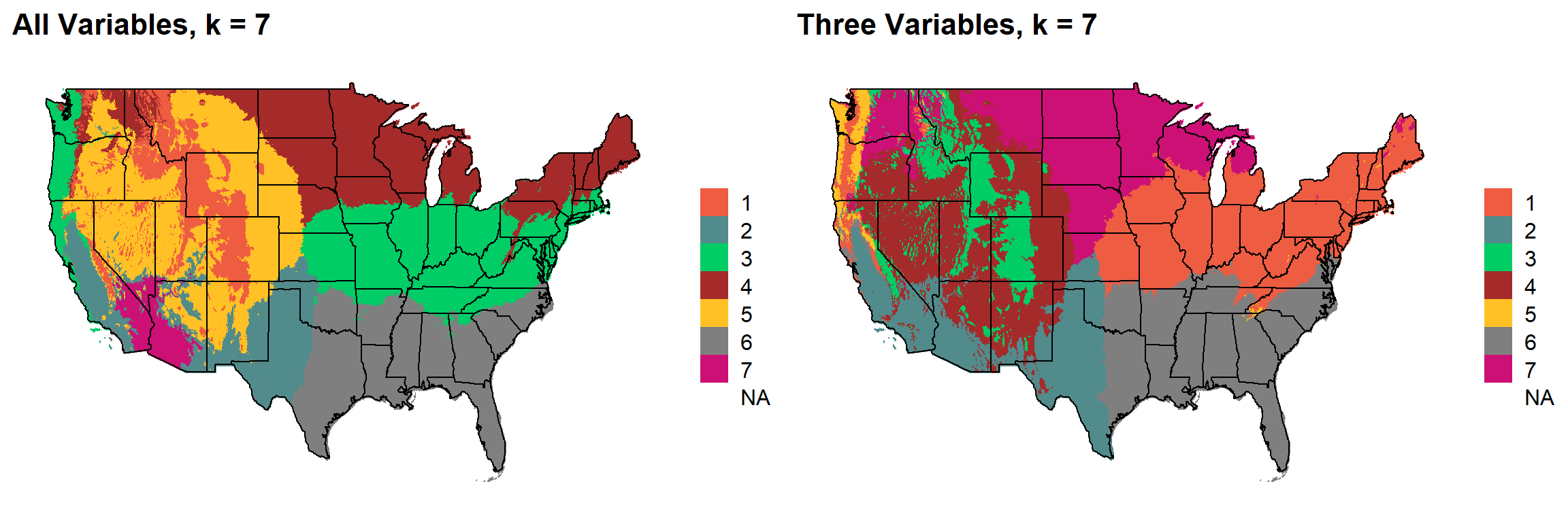
K = 8
plotlist[[7]]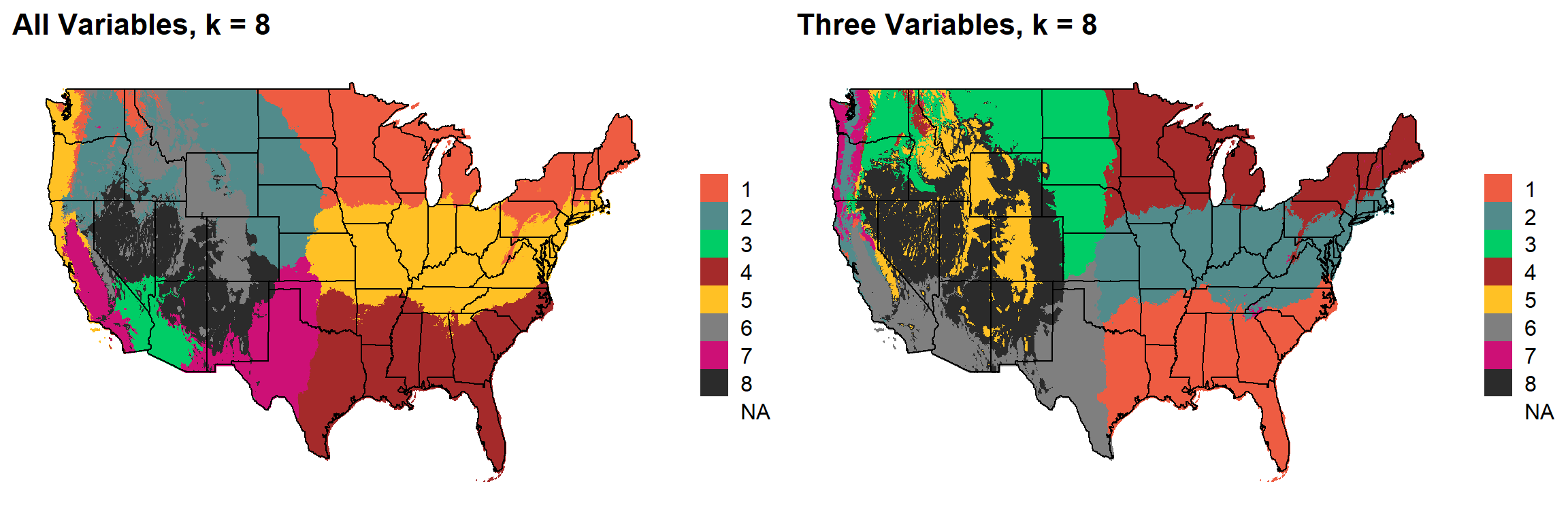
K = 9
plotlist[[8]]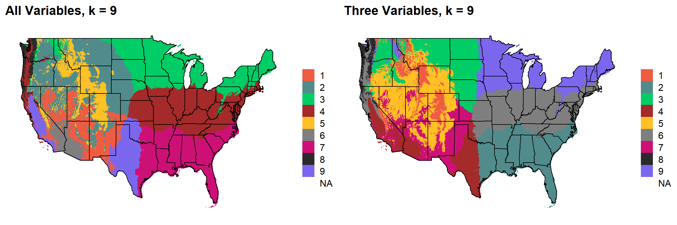
K = 10
plotlist[[9]]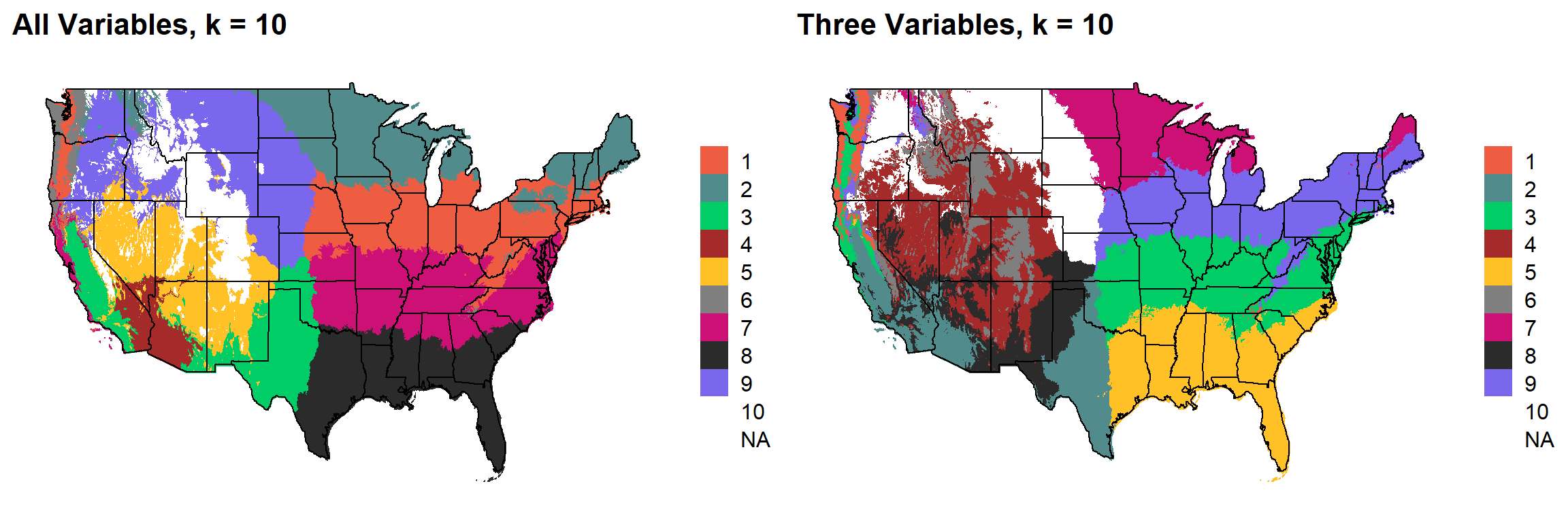
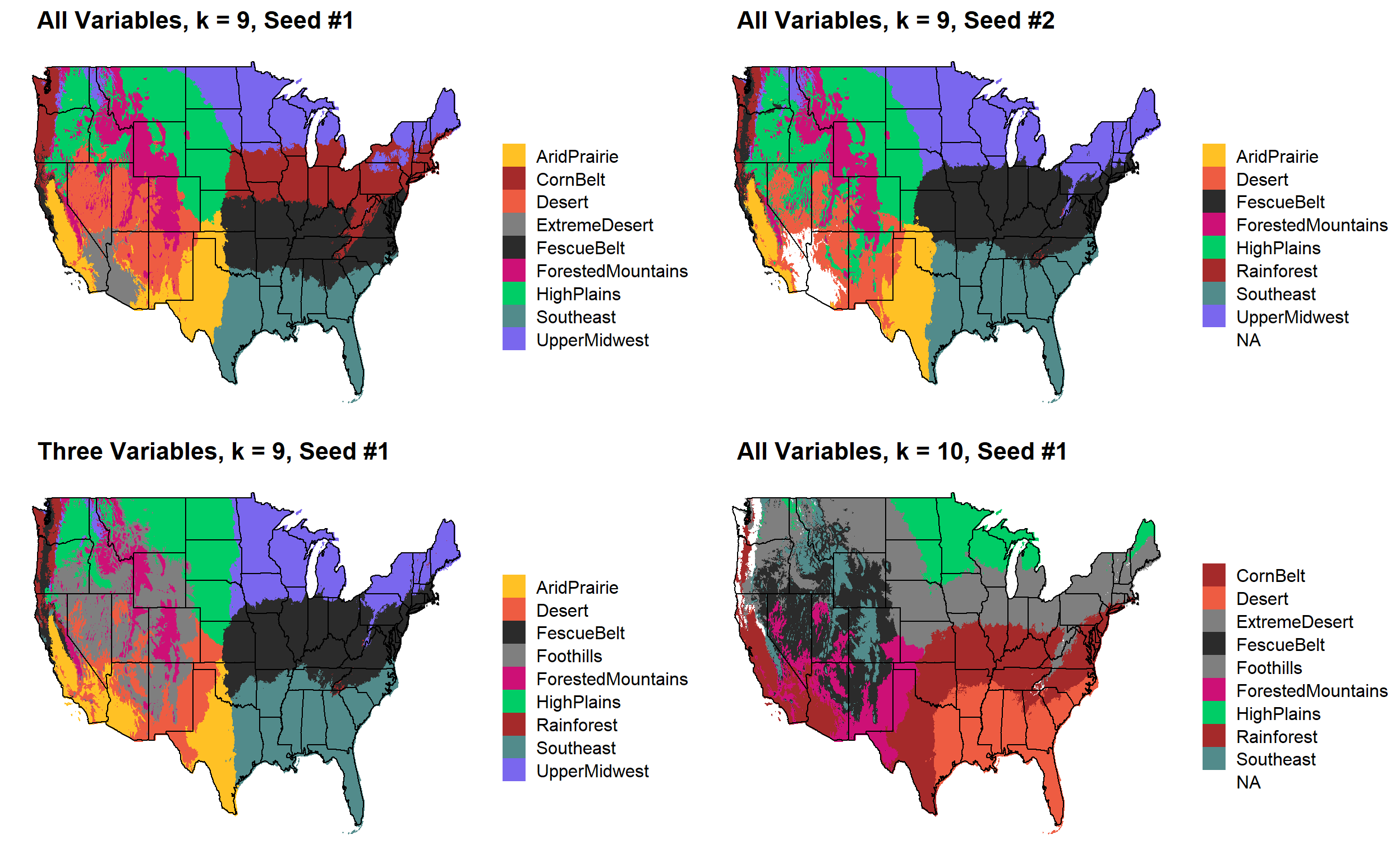
K = 9 ecoregion changes
I’d noticed eariler that there were major changes that occurred in the K = 9 map when using a different seed. In some cases, when using the these look similar to the original 3-variable ecoregions, and occasionally they break out the Fescue Belt into an extra region.
NOTE: The colors here aren’t corresponding from map to map because “zone number” is stochastically determined from run to run
Here, generate a k-means clustering map with K = 9 four times. I use each combination of all environmental variables and the three main variables and two different random seeds.
Using all variables actually makes more sense to me. Correlated variables don’t necessarily drive the assignments one way or another.
Observations: * More accurate “Fescue Belt” in ALL-Seed 1, that said, still likely too far West, not far enough North, disappears with Seed 2 * Rainforest ecoregion disappears with ALL-Seed 1 map (which is probably okay) * All-variable maps division of Dakotas tracks Missouri River (and a real chang in production environment) * ALL-Seed 1 is much less “granular” in elevation divisions. Should result in less weird “regional islands” due to (usually) elevation being created. * Not sure about the “rain line” in Texas, it certainly gets shifted to the West a bit * California is a bit strange in all of these maps still, but I think the differences that it picks up are real.
NOTE: There are definitely issues with coloring in the K = 10 for some reason.
My suggestion moving forward Use all-variable map (seed #1 version). I think that it makese divisions closer to how I’d divide the US based on what I know about these production environments. I’m interested in potentially partitioning out the Fescue Belt and Southeast further.
set.seed(325333)
k9_all =
  unsuperClass(stacked_raster,
               nSamples=2000,
               nClasses = 9,
               norm=TRUE,
               nStarts=5,
               clusterMap=FALSE) %>%
    .$map %>%
    as.data.frame(xy=TRUE) %>%
    mutate(layer = as.factor(layer)) %>%
    filter(!is.na(layer)) %>%
  mutate(region = case_when(layer == 1 ~ "HighPlains",
                            layer == 2 ~ "Desert",
                            layer == 3 ~ "Southeast",
                            layer == 4 ~ "CornBelt",
                            layer == 5 ~ "FescueBelt",
                            layer == 6 ~ "ForestedMountains",
                            layer == 7 ~ "UpperMidwest",
                            layer == 8 ~ "AridPrairie",
                            layer == 9 ~ "ExtremeDesert"))
#saveRDS(k9_all, "output/k9.allvars.seed1.rds")

k9_three =
  unsuperClass(threevar_stacked_raster,
               nSamples=2000,
               nClasses = 9,
               norm=TRUE,
               nStarts=5,
               clusterMap=FALSE) %>%
    .$map %>%
    as.data.frame(xy=TRUE) %>%
    mutate(layer = as.factor(layer)) %>%
    filter(!is.na(layer)) %>%
  mutate(region = case_when(layer == 7 ~ "HighPlains",
                            layer == 5 ~ "Desert",
                            layer == 2 ~ "Southeast",
                            layer == 8 ~ "Rainforest",
                            layer == 1 ~ "FescueBelt",
                            layer == 9 ~ "ForestedMountains",
                            layer == 6 ~ "UpperMidwest",
                            layer == 4 ~ "AridPrairie",
                            layer == 3 ~ "Foothills"))
#saveRDS(k9_three, "output/k9.threevars.seed1.rds")


set.seed(8675305)
k9_all_newseed =
  unsuperClass(stacked_raster,
               nSamples=2000,
               nClasses = 9,
               norm=TRUE,
               nStarts=5,
               clusterMap=FALSE) %>%
    .$map %>%
    as.data.frame(xy=TRUE) %>%
    mutate(layer = as.factor(layer)) %>%
    filter(!is.na(layer))%>%
  mutate(region = case_when(layer == 1 ~ "HighPlains",
                            layer == 5 ~ "Desert",
                            layer == 9 ~ "Southeast",
                            layer == 4 ~ "Rainforest",
                            layer == 7 ~ "FescueBelt",
                            layer == 2 ~ "ForestedMountains",
                            layer == 3 ~ "UpperMidwest",
                            layer == 8 ~ "AridPrairie",
                            layer == 3 ~ "ExtremeDesert"))
#saveRDS(k9_all_newseed, "output/k9.allvars.seed2.rds")

k9_three_newseed =
  unsuperClass(threevar_stacked_raster,
               nSamples=2000,
               nClasses = 9,
               norm=TRUE,
               nStarts=5,
               clusterMap=FALSE) %>%
    .$map %>%
    as.data.frame(xy=TRUE) %>%
    mutate(layer = as.factor(layer)) %>%
    filter(!is.na(layer))
saveRDS(k9_three_newseed, "output/k9.threevars.seed2.rds")


set.seed(325333)
k9_four =
  unsuperClass(fourvar_stacked_raster,
               nSamples=2000,
               nClasses = 9,
               norm=TRUE,
               nStarts=5,
               clusterMap=FALSE) %>%
    .$map %>%
    as.data.frame(xy=TRUE) %>%
    mutate(layer = as.factor(layer)) %>%
    filter(!is.na(layer)) %>%
    mutate(region = case_when(layer == 1 ~ "HighPlains",
                              layer == 2 ~ "Foothills",
                              layer == 3 ~ "Southeast",
                              layer == 4 ~ "FescueBelt",
                              layer == 5 ~ "Rainforest",
                              layer == 6 ~ "ForestedMountains",
                              layer == 7 ~ "UpperMidwest",
                              layer == 8 ~ "AridPrairie",
                              layer == 9 ~ "Desert"))


set.seed(325333)
k10 =
  unsuperClass(threevar_stacked_raster,
               nSamples=2000,
               nClasses = 10,
               norm=TRUE,
               nStarts=5,
               clusterMap=FALSE) %>%
    .$map %>%
    as.data.frame(xy=TRUE) %>%
    mutate(layer = as.factor(layer)) %>%
    filter(!is.na(layer))%>%
    mutate(region = case_when(layer == 1 ~ "HighPlains",
                              layer == 2 ~ "Desert",
                              layer == 3 ~ "Southeast",
                              layer == 4 ~ "CornBelt",
                              layer == 5 ~ "FescueBelt",
                              layer == 6 ~ "ForestedMountains",
                              layer == 6 ~ "UpperMidwest",
                              layer == 8 ~ "Rainforest",
                              layer == 9 ~ "ExtremeDesert",
                              layer == 10 ~ "Foothills"))

#saveRDS(k10, "output/k10.allvars.seed2.rds")

colorkey = c("HighPlains"="springgreen3", "UpperMidwest"="slateblue2", "Desert"="tomato2", "AridPrairie"="goldenrod1", "FescueBelt"="gray17", "Rainforest" = "brown", "CornBelt"="brown", "Southeast"="darkslategray4", "ForestedMountains"="deeppink3", "Foothills" = "gray50", "ExtremeDesert" = "gray50")
colour = c("10" = "white", "3"="springgreen3", "9"="slateblue2", "1"="tomato2", "5"="goldenrod1", "6"="gray50", "8"="gray17", "4"="brown", "2"="darkslategray4", "7"="deeppink3")


plot_grid(
  k9_all %>%
    kmeans_map(id = region, color = colorkey)+
      ggtitle(paste("    All Variables, k = 9, Seed #1")),
  k9_all_newseed %>%
    kmeans_map(id = region, color = colorkey)+
      ggtitle(paste("    All Variables, k = 9, Seed #2")),
  k9_three %>%
    kmeans_map(id = region, color = colorkey)+
      ggtitle(paste("    Three Variables, k = 9, Seed #1")),
  k10 %>%
    kmeans_map(id = region, color = colorkey)+
      ggtitle(paste("    All Variables, k = 10, Seed #1")),
  nrow = 2
  )
Comparing K=9 with different input variables
Three Variables
Temperature (mean), Precipitation, Elevation
k9_three %>%
  kmeans_map(id = region, color = colorkey)+
      ggtitle(paste("    Three Variables, k = 9, Seed #1"))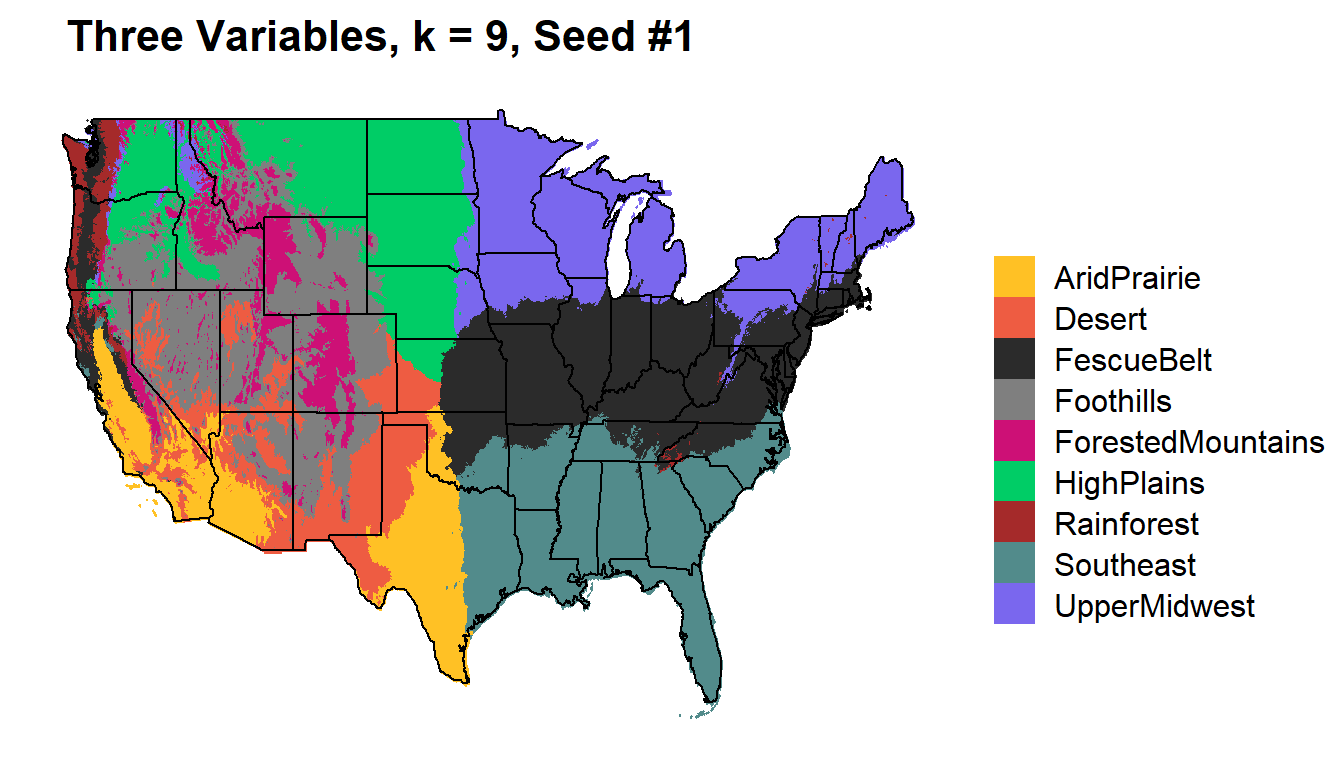
Four Variables
Temperature (mean), Precipitation, Elevation, Minimum Vapor Pressure
k9_four %>%
  kmeans_map(id = region, color = colorkey)+
      ggtitle(paste("    Four Variables, k = 9, Seed #1"))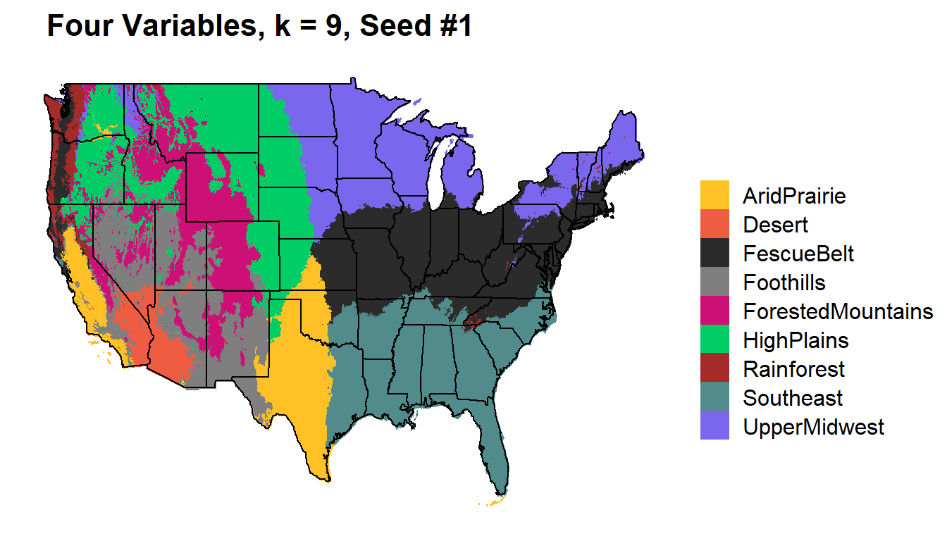
All Variables
Temperature (min, max, mean), Precipitation, DewPoint, Elevation, Vapor Pressure (min, max)
k9_all %>%
  kmeans_map(id = region, color = colorkey)+
      ggtitle(paste("    All Variables, k = 9, Seed #1"))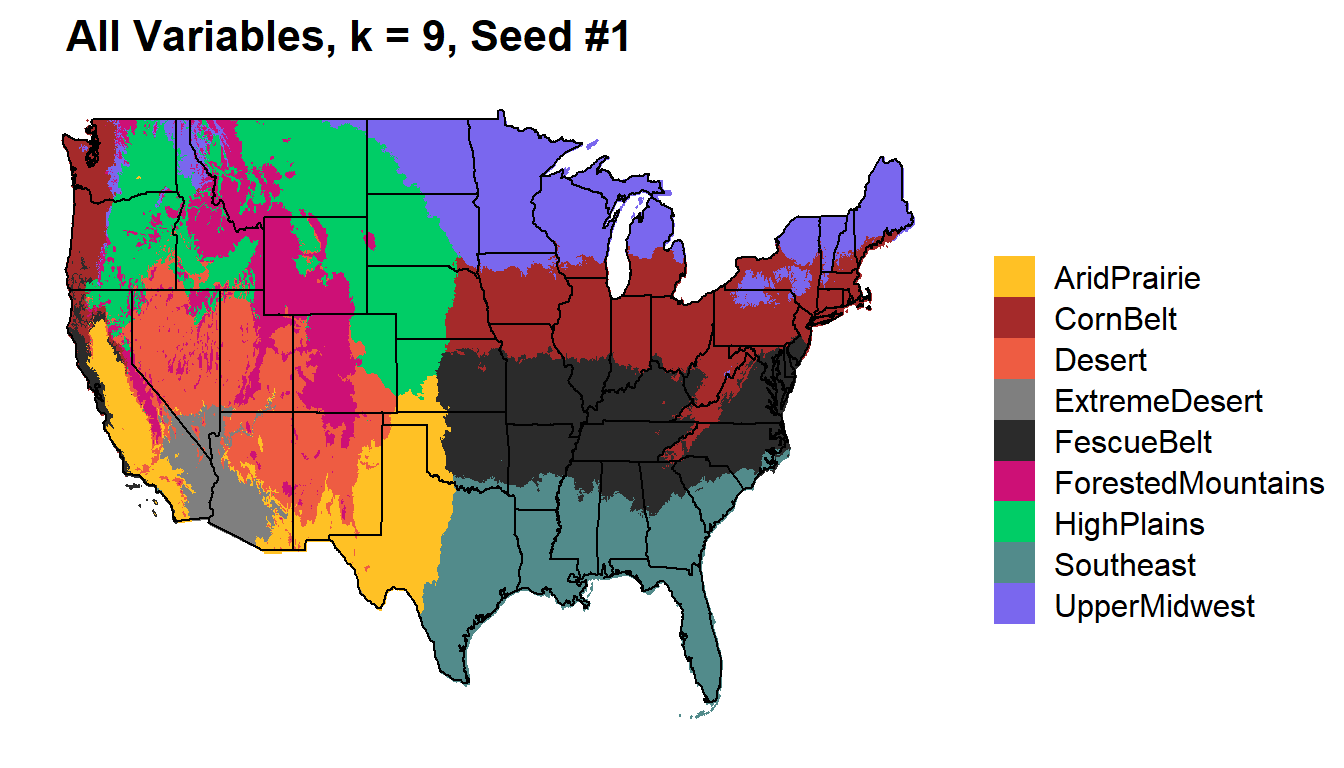
sessionInfo()R version 3.6.1 (2019-07-05)
Platform: x86_64-w64-mingw32/x64 (64-bit)
Running under: Windows 10 x64 (build 19041)
Matrix products: default
locale:
[1] LC_COLLATE=English_United States.1252
[2] LC_CTYPE=English_United States.1252
[3] LC_MONETARY=English_United States.1252
[4] LC_NUMERIC=C
[5] LC_TIME=English_United States.1252
attached base packages:
[1] stats graphics grDevices utils datasets methods base
other attached packages:
[1] forcats_0.5.0 stringr_1.4.0 dplyr_0.8.5 readr_1.3.1
[5] tidyr_1.0.3 tibble_3.0.1 tidyverse_1.3.0 here_0.1
[9] ggcorrplot_0.1.3 corrr_0.4.2 factoextra_1.0.7 ggplot2_3.3.0
[13] purrr_0.3.4 cowplot_1.0.0 ggthemes_4.2.0 maps_3.3.0
[17] RStoolbox_0.2.6 fpc_2.2-7 raster_3.3-7 rgdal_1.5-12
[21] sp_1.4-2 knitr_1.28 workflowr_1.6.2
loaded via a namespace (and not attached):
[1] colorspace_1.4-1 ggsignif_0.6.0 rio_0.5.16
[4] ellipsis_0.3.0 class_7.3-15 modeltools_0.2-23
[7] mclust_5.4.6 rprojroot_1.3-2 fs_1.4.1
[10] rstudioapi_0.11 ggpubr_0.4.0 farver_2.0.3
[13] ggrepel_0.8.2 flexmix_2.3-15 prodlim_2019.11.13
[16] fansi_0.4.1 lubridate_1.7.8 xml2_1.3.2
[19] codetools_0.2-16 splines_3.6.1 doParallel_1.0.15
[22] robustbase_0.93-6 jsonlite_1.6.1 pROC_1.16.2
[25] caret_6.0-86 broom_0.5.6 cluster_2.1.0
[28] kernlab_0.9-29 dbplyr_1.4.3 rgeos_0.5-3
[31] compiler_3.6.1 httr_1.4.1 backports_1.1.6
[34] assertthat_0.2.1 Matrix_1.2-17 cli_2.0.2
[37] later_1.0.0 htmltools_0.4.0 tools_3.6.1
[40] gtable_0.3.0 glue_1.4.0 reshape2_1.4.4
[43] Rcpp_1.0.4.6 carData_3.0-4 cellranger_1.1.0
[46] vctrs_0.2.4 nlme_3.1-140 iterators_1.0.12
[49] timeDate_3043.102 gower_0.2.2 xfun_0.13
[52] openxlsx_4.1.5 rvest_0.3.5 lifecycle_0.2.0
[55] rstatix_0.6.0 XML_3.99-0.3 DEoptimR_1.0-8
[58] MASS_7.3-51.4 scales_1.1.0 ipred_0.9-9
[61] hms_0.5.3 promises_1.1.0 parallel_3.6.1
[64] curl_4.3 yaml_2.2.1 geosphere_1.5-10
[67] rpart_4.1-15 stringi_1.4.6 highr_0.8
[70] foreach_1.5.0 zip_2.0.4 lava_1.6.7
[73] rlang_0.4.6 pkgconfig_2.0.3 prabclus_2.3-2
[76] evaluate_0.14 lattice_0.20-38 recipes_0.1.13
[79] labeling_0.3 tidyselect_1.0.0 plyr_1.8.6
[82] magrittr_1.5 R6_2.4.1 generics_0.0.2
[85] DBI_1.1.0 foreign_0.8-71 pillar_1.4.4
[88] haven_2.2.0 whisker_0.4 withr_2.2.0
[91] abind_1.4-5 survival_3.2-3 nnet_7.3-12
[94] car_3.0-8 modelr_0.1.7 crayon_1.3.4
[97] rmarkdown_2.1 grid_3.6.1 readxl_1.3.1
[100] data.table_1.12.8 git2r_0.27.1 ModelMetrics_1.2.2.2
[103] reprex_0.3.0 digest_0.6.25 diptest_0.75-7
[106] httpuv_1.5.2 stats4_3.6.1 munsell_0.5.0