DEG-analysis
unawaz1996
2023-03-14
Last updated: 2023-05-19
Checks: 6 1
Knit directory: NMD-analysis/
This reproducible R Markdown analysis was created with workflowr (version 1.7.0). The Checks tab describes the reproducibility checks that were applied when the results were created. The Past versions tab lists the development history.
Great! Since the R Markdown file has been committed to the Git repository, you know the exact version of the code that produced these results.
Great job! The global environment was empty. Objects defined in the global environment can affect the analysis in your R Markdown file in unknown ways. For reproduciblity it’s best to always run the code in an empty environment.
The command set.seed(20230314) was run prior to running
the code in the R Markdown file. Setting a seed ensures that any results
that rely on randomness, e.g. subsampling or permutations, are
reproducible.
Great job! Recording the operating system, R version, and package versions is critical for reproducibility.
Nice! There were no cached chunks for this analysis, so you can be confident that you successfully produced the results during this run.
Using absolute paths to the files within your workflowr project makes it difficult for you and others to run your code on a different machine. Change the absolute path(s) below to the suggested relative path(s) to make your code more reproducible.
| absolute | relative |
|---|---|
| /home/neuro/Documents/NMD_analysis/Analysis/NMD-analysis/output/DEG/Thesis_figures/Gene_PCA.svg | output/DEG/Thesis_figures/Gene_PCA.svg |
| /home/neuro/Documents/NMD_analysis/Analysis/NMD-analysis/output/DEG/Thesis_figures/total_DEG.svg | output/DEG/Thesis_figures/total_DEG.svg |
| /home/neuro/Documents/NMD_analysis/Analysis/NMD-analysis/output/DEG/Thesis_figures/ratio_DEG.svg | output/DEG/Thesis_figures/ratio_DEG.svg |
| /home/neuro/Documents/NMD_analysis/Analysis/NMD-analysis/output/DEG/Thesis_figures/UPF3B_KD_volcano.svg | output/DEG/Thesis_figures/UPF3B_KD_volcano.svg |
| /home/neuro/Documents/NMD_analysis/Analysis/NMD-analysis/output/DEG/Thesis_figures/UPF3_venn.svg | output/DEG/Thesis_figures/UPF3_venn.svg |
| /home/neuro/Documents/NMD_analysis/Analysis/NMD-analysis/output/DEG/Thesis_figures/UPF3_corr.svg | output/DEG/Thesis_figures/UPF3_corr.svg |
| /home/neuro/Documents/NMD_analysis/Analysis/NMD-analysis/output/DEG/Thesis_figures/UPF3B_corr.svg | output/DEG/Thesis_figures/UPF3B_corr.svg |
| /home/neuro/Documents/NMD_analysis/Analysis/NMD-analysis/output/DEG/Thesis_figures/UPF3A_corr.svg | output/DEG/Thesis_figures/UPF3A_corr.svg |
Great! You are using Git for version control. Tracking code development and connecting the code version to the results is critical for reproducibility.
The results in this page were generated with repository version e526ece. See the Past versions tab to see a history of the changes made to the R Markdown and HTML files.
Note that you need to be careful to ensure that all relevant files for
the analysis have been committed to Git prior to generating the results
(you can use wflow_publish or
wflow_git_commit). workflowr only checks the R Markdown
file, but you know if there are other scripts or data files that it
depends on. Below is the status of the Git repository when the results
were generated:
Ignored files:
    Ignored:    .Rhistory
    Ignored:    .Rproj.user/
    Ignored:    analysis/Differential-transcript-usage.nb.html
    Ignored:    analysis/Enichment-analysis-fgsea.nb.html
    Ignored:    analysis/Enichment-analysis-goseq.nb.html

Untracked files:
    Untracked:  PCA.png
    Untracked:  PCA_plot.pdf
    Untracked:  PCA_transcript.png
    Untracked:  analysis/Differential-transcript-usage.Rmd
    Untracked:  analysis/UPF3B_KD.Rmd
    Untracked:  analysis/transcript-preprocessing.Rmd
    Untracked:  code/eisaR.R
    Untracked:  code/external_code/
    Untracked:  data/LTK_Sample Metafile_V3.txt
    Untracked:  data/Mus_musculus.GRCm39.105__nifs.tsv
    Untracked:  data/data.txt
    Untracked:  data/data2.txt
    Untracked:  data/fastqc/
    Untracked:  data/nif_output/
    Untracked:  data/samples.txt
    Untracked:  output/DEG-limma-results.Rda
    Untracked:  output/DEG-list.Rda
    Untracked:  output/DEG/
    Untracked:  output/EISA/
    Untracked:  output/For_presentation/
    Untracked:  output/ISAR/
    Untracked:  output/QC/
    Untracked:  output/Transcript/
    Untracked:  output/isoformSwitchAnalyzeR_isoform_AA_complete.fasta
    Untracked:  output/isoformSwitchAnalyzeR_isoform_AA_subset_1_of_3.fasta
    Untracked:  output/isoformSwitchAnalyzeR_isoform_AA_subset_2_of_3.fasta
    Untracked:  output/isoformSwitchAnalyzeR_isoform_AA_subset_3_of_3.fasta
    Untracked:  output/isoformSwitchAnalyzeR_isoform_nt.fasta
    Untracked:  output/limma-matrices.Rda
    Untracked:  tmp/

Unstaged changes:
    Modified:   analysis/Differential-transcript-expression.Rmd
    Modified:   analysis/Enichment-analysis-fgsea.Rmd
    Modified:   analysis/Quality-control.Rmd
    Modified:   analysis/RNA-stability.Rmd
    Modified:   analysis/_site.yml
    Modified:   code/functions.R
    Modified:   code/libraries.R
Note that any generated files, e.g. HTML, png, CSS, etc., are not included in this status report because it is ok for generated content to have uncommitted changes.
These are the previous versions of the repository in which changes were
made to the R Markdown (analysis/DEG-analysis.Rmd) and HTML
(docs/DEG-analysis.html) files. If you’ve configured a
remote Git repository (see ?wflow_git_remote), click on the
hyperlinks in the table below to view the files as they were in that
past version.
| File | Version | Author | Date | Message |
|---|---|---|---|---|
| Rmd | e526ece | unawaz1996 | 2023-05-19 | wflow_publish(c("analysis/index.Rmd", "analysis/DEG-analysis.Rmd")) |
| html | a23bb43 | unawaz1996 | 2023-05-19 | Build site. |
| Rmd | ac69819 | unawaz1996 | 2023-05-19 | wflow_publish(c("analysis/index.Rmd", "analysis/DEG-analysis.Rmd")) |
| html | 4e55d99 | unawaz1996 | 2023-05-12 | Build site. |
| html | bff9b8f | unawaz1996 | 2023-05-12 | Build site. |
| Rmd | 05f4d8c | unawaz1996 | 2023-05-12 | wflow_publish(c("analysis/index.Rmd", "analysis/DEG-analysis.Rmd", |
| html | f8ef81a | unawaz1996 | 2023-05-11 | Build site. |
| Rmd | 582094c | unawaz1996 | 2023-05-11 | wflow_publish(c("analysis/index.Rmd", "analysis/DEG-analysis.Rmd")) |
| html | 401069b | unawaz1996 | 2023-05-04 | Build site. |
| Rmd | 606fc38 | unawaz1996 | 2023-05-04 | wflow_publish(c("analysis/index.Rmd", "analysis/DEG-analysis.Rmd")) |
| html | a9a5164 | unawaz1996 | 2023-03-14 | Build site. |
| Rmd | 7e6ee7a | unawaz1996 | 2023-03-14 | Add main result page to navbar |
| html | 6b613fc | unawaz1996 | 2023-03-14 | Build site. |
| html | 780272b | unawaz1996 | 2023-03-14 | Build site. |
| html | 5a8cba6 | unawaz1996 | 2023-03-14 | Build site. |
| Rmd | 4856ece | unawaz1996 | 2023-03-14 | Add DEG analysis |
source("code/plots.R")
source("code/functions.R")
source("code/libraries.R")
library(biomaRt)
library(nVennR)
library(eulerr)
library(ggsci)
Introduction
Count data
Gene-level count data was retrieved from salmon files by
tximport into a DGEList object. During this process, genes
were removed if
- They were not considered as detectable (TPM < 0.5 in > 3 samples)
- They did not contain any annotation
These filtering steps returned gene-level counts for 10,957 genes.
# Quality control of genes
salmon.files = ("/home/neuro/Documents/NMD_analysis/Analysis/Results/Salmon")
md.files = "data/LTK_Sample Metafile_V3.txt"

# Loading data
txdf = transcripts(EnsDb.Mmusculus.v79, return.type="DataFrame")
tx2gene = as.data.frame(txdf[,c("tx_id","gene_id")])

salmon = list.files(salmon.files, pattern = "transcripts$", full.names = TRUE)
all_files = file.path(salmon, "quant.sf")
names(all_files) <- paste(c(212:229))

txi_genes <- tximport(all_files, type="salmon", txOut=FALSE,
                      countsFromAbundance="scaledTPM", tx2gene = tx2gene, ignoreTxVersion = TRUE, ignoreAfterBar = TRUE)


md = read.table(md.files, header= TRUE) %>%  mutate(files = file.path(salmon, "quant.sf"))
md$Group = factor(md$Group)
md$Sample = as.character(md$Sample)
group_cols <- hcl.colors(
n = length(unique(md$Group)),
palette = "Zissou 1"
) %>%
setNames(unique(md$Group))keep = (rowSums(txi_genes$abundance >= .5 ) >= 3)
exp_den = txi_genes$counts %>% cpm(log=TRUE) %>%
melt() %>%
dplyr::filter(is.finite(value)) %>%
ggplot(aes(x=value, color = as.character(Var2))) +
geom_density() +
ggtitle("Before filtering") +
labs(x = "logCPM", y = "Proportion of Genes") +
theme_bw() +
theme(legend.position = "none")
exp_den_filt = txi_genes$counts %>%
cpm(log=TRUE) %>%
magrittr::extract(keep,) %>%
melt() %>%
dplyr::filter(is.finite(value)) %>%
ggplot(aes(x=value, color = as.character(Var2))) +
geom_density() +
ggtitle("After filtering") +
labs(x = "logCPM", y = "Proportion of Genes") + theme_bw() +
theme(legend.position = "none")
grid.arrange(exp_den,exp_den_filt, ncol=2 )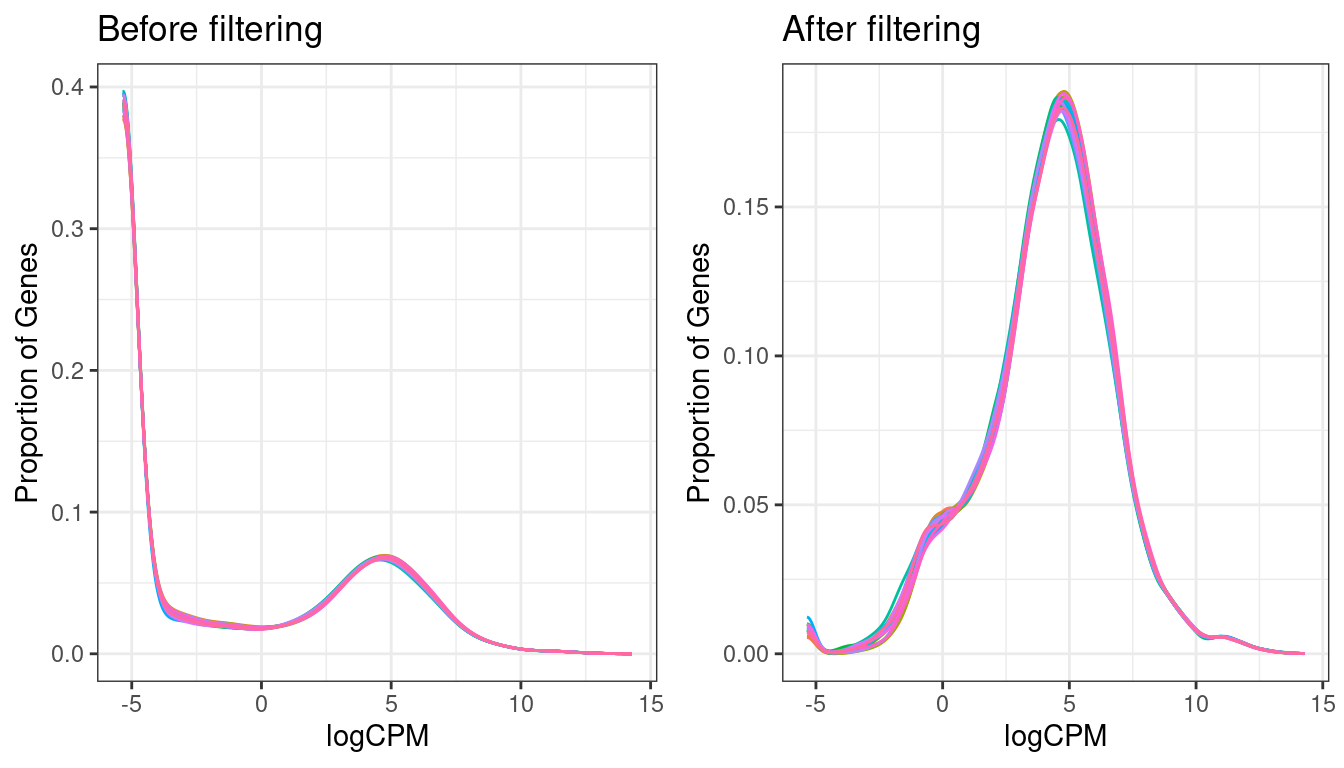
Expression density plots for all samples before and after filtering, showing logCPM values.
txi_genes_filtered = txi_genes$counts[keep,] %>%
    as.data.frame() %>%
    rownames_to_column("geneID") %>%
    mutate(geneName = mapIds(org.Mm.eg.db, keys=.$geneID,
                             column="SYMBOL",keytype="ENSEMBL",
                         multiVals="first")) %>%
    drop_na(geneName) %>%
    column_to_rownames("geneID") %>% dplyr::select(-geneName)
Analysis
PCA
pca = log2(txi_genes$abundance[keep,]  + 10^-6 ) %>%
    t() %>%
    prcomp(scale = TRUE)

pcaVars <- percent_format(0.1)(summary(pca)$importance["Proportion of Variance",])

gene_pca = pca$x[,1:2] %>%
    as.data.frame()  %>%
    cbind(md) %>%
    as.tibble() %>%
    ggplot(aes(PC1, PC2, shape = Condition_UPF3B, label = Condition_UPF3B, color=Group)) +
    geom_point(size = 11.5) +
    theme_bw() + scale_shape_manual(values = c(0,16)) + labs(shape="UPF3B status", colour= "Samples") +
    theme(axis.title.y = element_text(size = 12), axis.title.x = element_text(size = 12),
          axis.text = element_text(size = 10)) +
    xlab(paste0("Principal Component 1 (28.1%)")) + ylab("Principal Component 2 (16.6%)") +
    scale_color_manual(values = c("#FCC98A","#6E74B4", "#E12F8F","#EA2A5F", "#FD9675", "#2F124B"),
                      labels = c("UPF3A_KD_UPF3B_KD" = "Double KD", "UPF3A_KD" = "UPF3A KD",
                                                                   "UPF3B_KD" = "UPF3B KD", "UPF3A_OE" = "UPF3A OE",
                                                                   "UPF3A_OE_UPF3B_KD" = "UPF3A OE UPF3B KD")) +
  labs(x = paste0("PC1 (", pcaVars[["PC1"]], ")"),
    y = paste0("PC2 (", pcaVars[["PC2"]], ")"))

#ggsave(filename = "/home/neuro/Documents/NMD_analysis/Analysis/NMD-analysis/output/DEG/Thesis_figures/Gene_PCA.svg", plot = gene_pca,
#       units = c("in"), width = 6.65, height = 5.60)
The principal component analysis was performed using the logCPM values from each sample. Each group appears to be clustering together. UPF3A over-expression is clustering with Controls, whereas the UPF3B KD samples are clustering closely with UPF3A overexpression in UPF3B KD files.
Boxplots of gene expression and library size
txi_genes$abundance[keep,] %>%
    as.data.frame() %>%
    gather(sample,value) %>%
    ggplot(aes(x=sample, y = log(value), fill = sample)) + geom_boxplot() +
    ylab("Log(TPM)") + xlab("Samples") +
    theme_bw() + theme(legend.position = "none") + scale_fill_manual(values = hydrangea[1:18])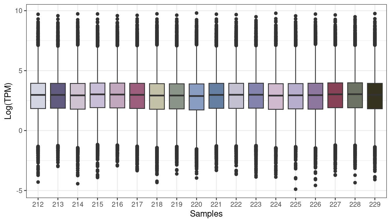
# Library size

countsSum <- colSums(txi_genes$counts) # library size
countsSum %>% melt() %>% rownames_to_column("Sample") %>%
    ggplot(aes(x=Sample, y = value)) + geom_bar(stat = "identity") + ylab("Library size") +
    theme_bw()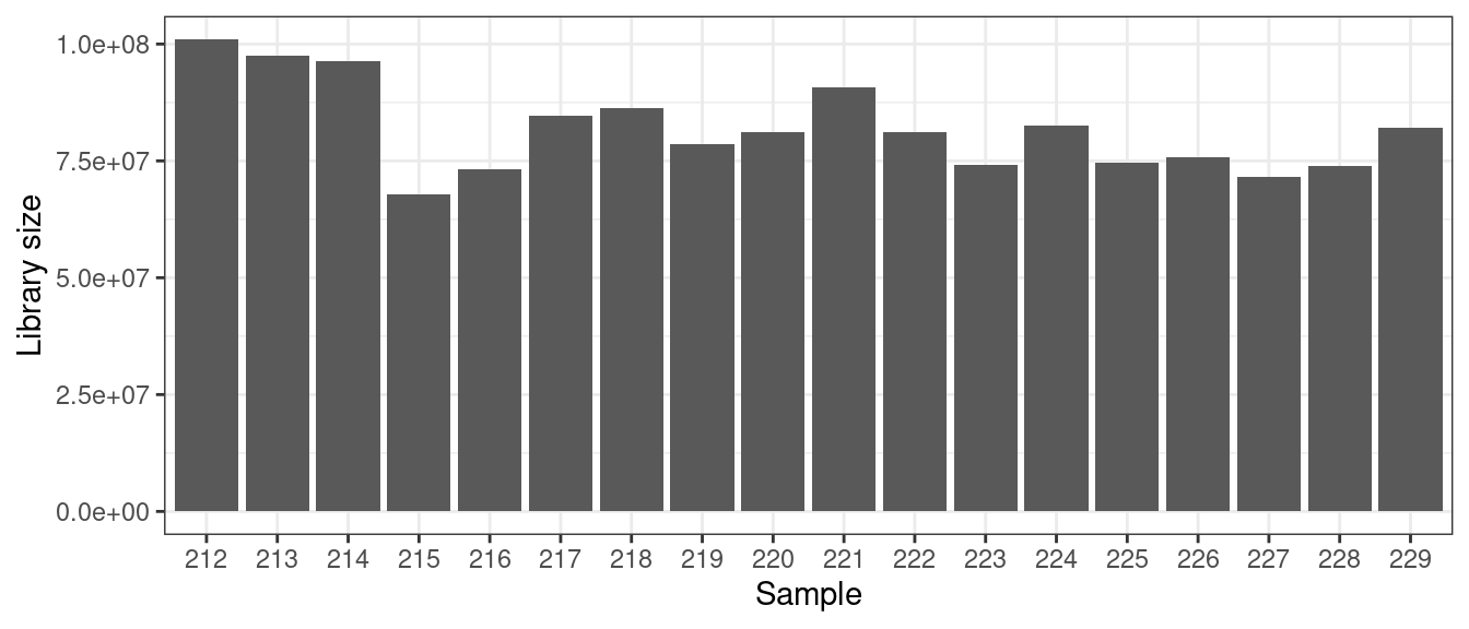
#max(countsSum) / min(countsSum)Differential gene expression using limma
Model description
In this analysis, we are interested in seeing how the knockdowns
behave differently to controls. Given the quality and clustering of the
data, we will perform five pairwise comparisons using limma
where all conditions (KD/OE) will be compared to controls.
y <- DGEList(txi_genes_filtered)


design <- model.matrix(~0+Group, data = md) %>%
    set_colnames(gsub(pattern = "Group", replacement ="", x = colnames(.)))

contrasts <- makeContrasts(levels = colnames(design),
                           UPF3B_vs_Control = UPF3B_KD - Control,
                           UPF3A_vs_Control = UPF3A_KD - Control,
                           UPF3A_OE_vs_Control = UPF3A_OE - Control,
                           DoubleKD_vs_Control = UPF3A_KD_UPF3B_KD - Control,
                           UPF3A_OE_UPF3B_KD_vs_Control = UPF3A_OE_UPF3B_KD - Control)
y <- calcNormFactors(y)
v <- voom(y, design)
fit = lmFit(v, design) %>%
contrasts.fit(contrasts) %>%
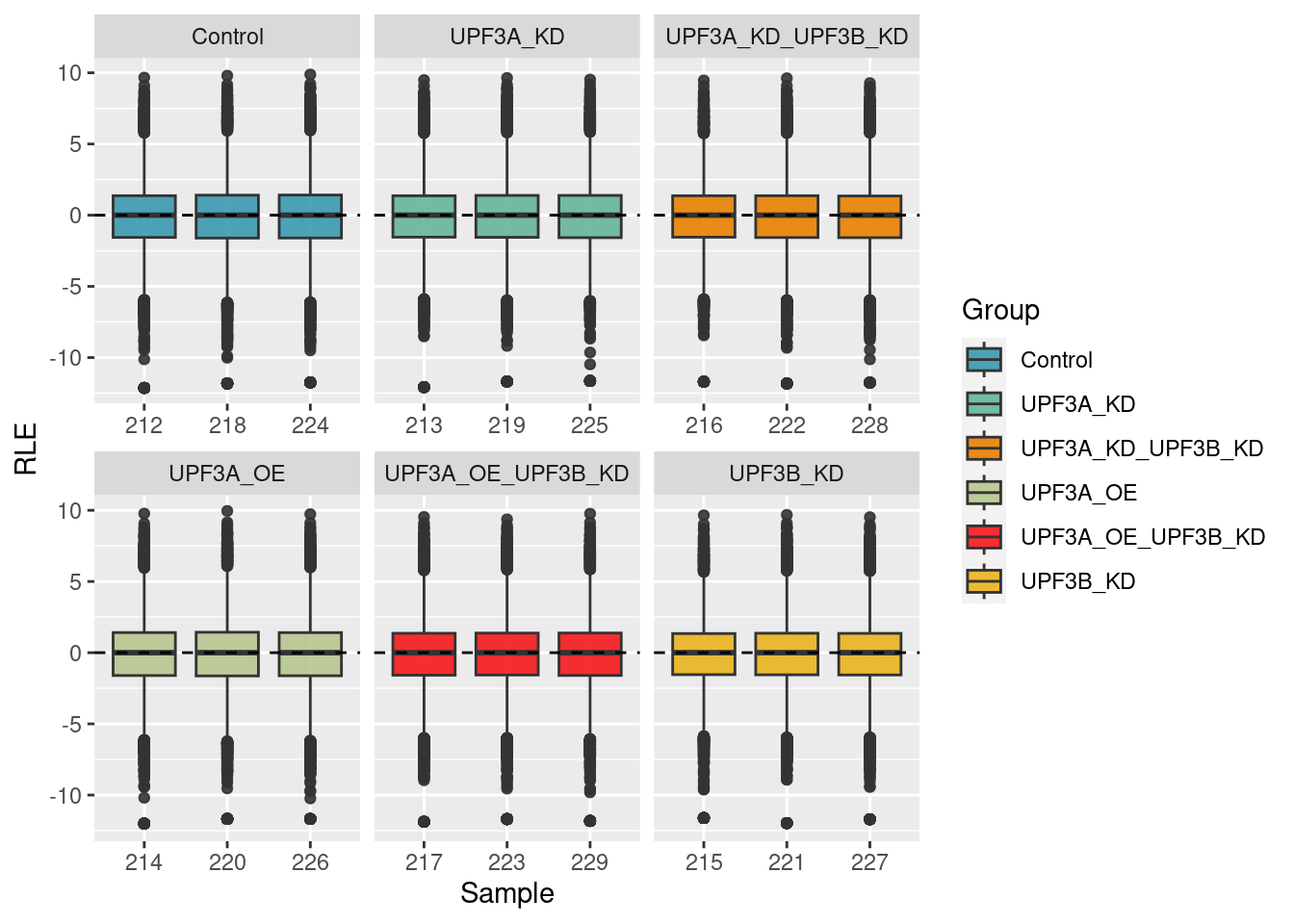
eBayes()v$E %>%
as.data.frame() %>%
pivot_longer(
cols = everything(), names_to = "Sample", values_to = "logCPM"
) %>%
left_join(md) %>%
group_by(Sample) %>%
mutate(RLE = logCPM - median(logCPM))%>%
ggplot(aes(Sample, RLE, fill = Group)) +
geom_boxplot(alpha = 0.9) +
geom_hline(yintercept = 0, linetype = 2) +
facet_wrap(~Group, scales = "free_x") +
scale_fill_manual(values = group_cols) +
labs(
x = "Sample", fill = "Group"
)
| Version | Author | Date |
|---|---|---|
| 401069b | unawaz1996 | 2023-05-04 |
## QC plots - deciding log2FC thresholds
results <- decideTests(fit, p.value = 0.05, adjust.method = "fdr", method= "global")
limma_results = write_fit(fit, results= results, adjust = "fdr") %>%
    rownames_to_column("ensembl_gene_id") %>%
    mutate(gene = mapIds(org.Mm.eg.db, keys=ensembl_gene_id,  column="SYMBOL",keytype="ENSEMBL", multiVals="first"),
           entrez = mapIds(org.Mm.eg.db, keys=ensembl_gene_id,  column="ENTREZID",keytype="ENSEMBL", multiVals="first")) %>% drop_na(entrez)


gene_expression_density = data.frame()
comparisons =c("UPF3B_vs_Control", "UPF3A_vs_Control",  "UPF3A_OE_vs_Control",
               "DoubleKD_vs_Control", "UPF3A_OE_UPF3B_KD_vs_Control")

for (c in comparisons) {
  sig_genes = limma_results %>% as.data.frame() %>%
    dplyr::select(contains("Coef"), contains ("p.value.adj"), contains(c)) %>%
  dplyr::filter(p.value.adj.UPF3B_vs_Control < 0.05) %>%
  dplyr::select(contains("Coef")) %>%
  dplyr::select(contains("UPF3B_vs_Control")) %>% melt()
  gene_expression_density = rbind(gene_expression_density, sig_genes )

}


#ggplot(aes(x=Coef.UPF3B_vs_Control)) +
 # geom_histogram(aes(y=..density..), colour="black", fill="white") +
 # geom_density(alpha=.2, fill="#FF6666") + geom_vline(xintercept =c(log2(1.5), -log2(1.5)),color="red", linetype = "dashed") +
#  theme_bw() + ylab("Density")
results <- decideTests(fit, p.value = 0.05, adjust.method = "fdr", method= "global", lfc = log2(1.5))
limma_results = write_fit(fit, results= results, adjust = "fdr") %>%
rownames_to_column("ensembl_gene_id") %>%
mutate(gene = mapIds(org.Mm.eg.db, keys=ensembl_gene_id, column="SYMBOL",keytype="ENSEMBL", multiVals="first"),
entrez = mapIds(org.Mm.eg.db, keys=ensembl_gene_id, column="ENTREZID",keytype="ENSEMBL", multiVals="first")) %>% drop_na(entrez)
#save(limma_results, file="/home/neuro/Documents/NMD_analysis/Analysis/Results/DEGs/DEG-limma-results.Rda")
#save(results, fit,y,v,contrasts, design, contrasts, file = "/home/neuro/Documents/NMD_analysis/Analysis/Results/DEGs/limma-matrices.Rda")DEGenes <- list()
DEGenes[["UPF3B_vs_Control"]] <- limma_results %>%
dplyr::filter(Res.UPF3B_vs_Control != 0, abs(Coef.UPF3B_vs_Control) > log2(1.5))
DEGenes[["UPF3A_vs_Control"]] <- limma_results %>%
dplyr::filter(Res.UPF3A_vs_Control != 0, abs(Coef.UPF3A_vs_Control) > log2(1.5))
DEGenes[["UPF3A_OE_vs_Control"]] <- limma_results %>%
dplyr::filter(Res.UPF3A_OE_vs_Control != 0, abs(Coef.UPF3A_OE_vs_Control) > log2(1.5)) %>%
arrange(p.value.UPF3A_OE_vs_Control)
DEGenes[["DoubleKD_vs_Control"]] <- limma_results %>%
dplyr::filter(Res.DoubleKD_vs_Control != 0, abs(Coef.DoubleKD_vs_Control) > log2(1.5)) %>%
arrange(p.value.DoubleKD_vs_Control)
DEGenes[["UPF3A_OE_UPF3B_KD_vs_Control"]] <- limma_results %>%
dplyr::filter(Res.UPF3A_OE_UPF3B_KD_vs_Control != 0, abs(Coef.UPF3A_OE_UPF3B_KD_vs_Control) > log2(1.5)) %>%
arrange(p.value.UPF3A_OE_UPF3B_KD_vs_Control)
#write.xlsx(DEGenes, "NMD-DEG-limma.xlsx")
#save(DEGenes, file="/home/neuro/Documents/NMD_analysis/Analysis/Results/DEGs/DEG-list.Rda")Total number of DEGs
summary(results) UPF3B_vs_Control UPF3A_vs_Control UPF3A_OE_vs_Control
Down 102 67 20
NotSig 10458 10464 10849
Up 316 345 7
DoubleKD_vs_Control UPF3A_OE_UPF3B_KD_vs_Control
Down 216 121
NotSig 9923 10535
Up 737 220summary_DEG = summary(results) %>% melt() %>%
dplyr::filter(Var1 != "NotSig")
summary_DEG$Var1 = factor(summary_DEG$Var1, levels = c("Up", "Down"))
summary_DEG$Var2 = factor(summary_DEG$Var2, levels = c("UPF3B_vs_Control",
"UPF3A_vs_Control",
"DoubleKD_vs_Control",
"UPF3A_OE_vs_Control",
"UPF3A_OE_UPF3B_KD_vs_Contro"))
summary_DEG = summary_DEG %>%
ggplot(aes(x=Var2, y = value, fill=Var1)) +
geom_bar(stat = "identity", colour = "white", width = .75) +
theme_bw() +
theme(axis.text.x = element_text(angle = 70, hjust=1, face = "bold", size=10),
legend.position = "bottom",
legend.title= element_blank(), axis.title.y = element_text(size = 12),
axis.text.y = element_text(size = 12, face = "bold")) +
scale_fill_manual(values = c("#EA2A5F", "#2F124B")) +
ylab("# Differentially expressed genes") + xlab("") + scale_x_discrete(labels=c("DoubleKD_vs_Control" = "Double KD", "UPF3A_vs_Control" = "UPF3A KD",
"UPF3B_vs_Control" = "UPF3B KD", "UPF3A_OE_vs_Control" = "UPF3A OE",
"UPF3A_OE_UPF3B_KD_vs_Control" = "UPF3A OE UPF3B KD"))
summary_DEG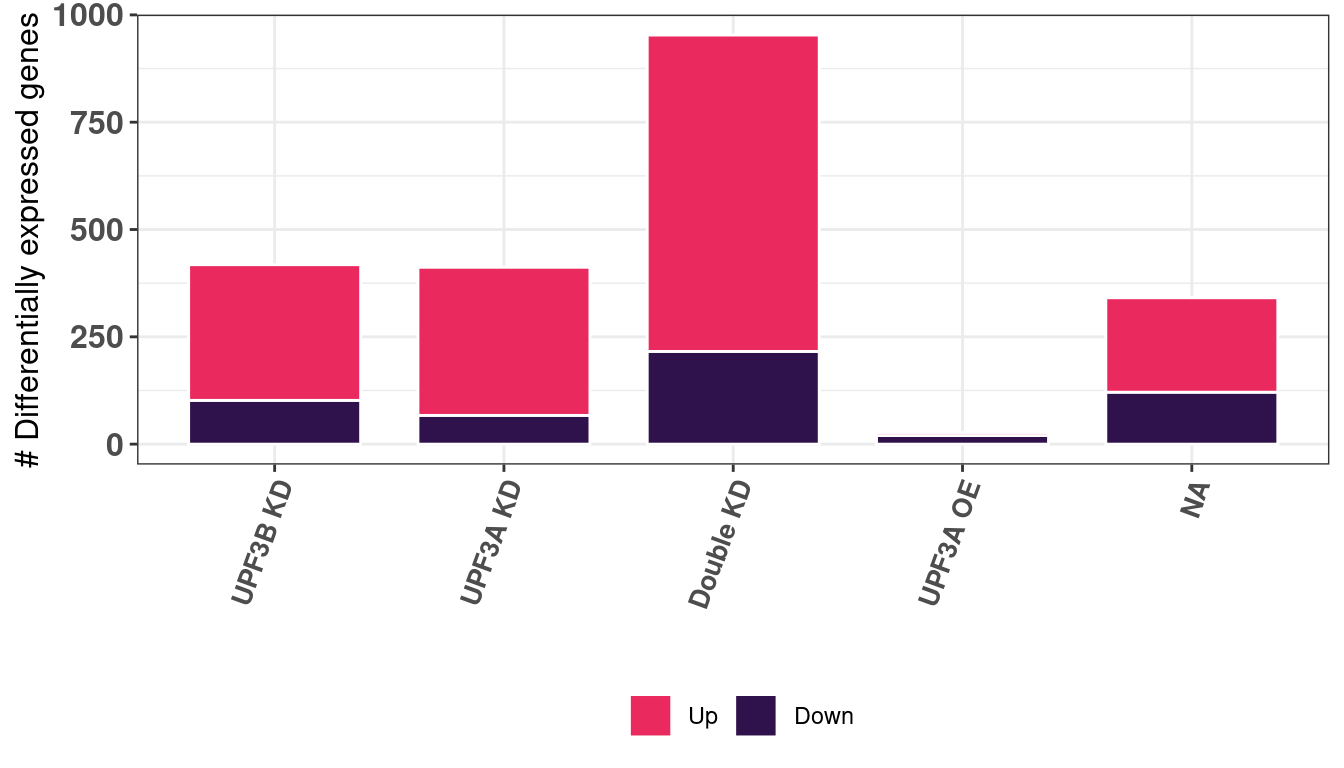
#ggsave(filename = "/home/neuro/Documents/NMD_analysis/Analysis/NMD-analysis/output/DEG/Thesis_figures/total_DEG.svg", plot = #summary_DEG,
#       units = c("in"), height = 5.31, width = 4.48)
ratios = data.frame()
for (c in comparisons){
temp = summary(results) %>%
melt() %>%
dplyr::filter(Var2 == c, Var1 != "NotSig")
ratio= temp$value[2]/temp$value[1]
ratio = data.frame(Comparisons = c,
ratio = ratio)
ratios = rbind(ratios, ratio)
}
ratios$Comparisons = factor(ratios$Comparisons, levels = c("UPF3B_vs_Control",
"UPF3A_vs_Control",
"DoubleKD_vs_Control",
"UPF3A_OE_vs_Control",
"UPF3A_OE_UPF3B_KD_vs_Control"))
ratios_fig =ratios %>%
ggplot(aes(x =Comparisons, y = ratio, fill = Comparisons)) +
geom_bar(stat = "identity", colour = "white", width = .75) +
theme_classic() +
theme(axis.text.x = element_text(angle = 70, hjust=1, face = "bold"),
legend.position = "none",
legend.title= element_blank(), axis.title.y = element_text(size = 12),
axis.text.y = element_text(size = 14, face = "bold")) +
scale_fill_manual(values = c("#2F124B","#EA2A5F","#6E74B4","#E12F8F", "#FD9675")) +
ylab("ratio up/down") + xlab("") + scale_x_discrete(labels=c("DoubleKD_vs_Control" = "Double KD", "UPF3A_vs_Control" = "UPF3A KD",
"UPF3B_vs_Control" = "UPF3B KD", "UPF3A_OE_vs_Control" = "UPF3A OE",
"UPF3A_OE_UPF3B_KD_vs_Control" = "UPF3A OE UPF3B KD"))
ratios Comparisons ratio
1 UPF3B_vs_Control 3.098039
2 UPF3A_vs_Control 5.149254
3 UPF3A_OE_vs_Control 0.350000
4 DoubleKD_vs_Control 3.412037
5 UPF3A_OE_UPF3B_KD_vs_Control 1.818182#ggsave(filename = "/home/neuro/Documents/NMD_analysis/Analysis/NMD-analysis/output/DEG/Thesis_figures/ratio_DEG.svg", plot = #ratios_fig,
# units = c("in"), height = 3.30, width = 4.48)After performing pairwise differential gene expression analysis, we can see that majority of all significantly expressed genes in all contrasts are up-regulated. Overall, we find that a total of 395 genes are differentially expressed between UPF3B KD and controls. 388 genes are differentially expressed between UPF3A KD vs Controls.
Overlapping DEGs
## Venn diagram and table representing each venn diagram with gene name and its results
ven <- venndetail(list("UPF3B KD" = DEGenes$UPF3B_vs_Control$gene,
                       "UPF3A KD" = DEGenes$UPF3A_vs_Control$gene,
                    "Double KD" = DEGenes$DoubleKD_vs_Control$gene,
                    "UPF3A OE" = DEGenes$UPF3A_OE_vs_Control$gene,
                  "UPF3A OE, UPF3B KD" = DEGenes$UPF3A_OE_UPF3B_KD_vs_Control$gene))
x=list("UPF3B KD" = DEGenes$UPF3B_vs_Control$ensembl_gene_id,
"UPF3A KD" = DEGenes$UPF3A_vs_Control$ensembl_gene_id,
"Double KD" = DEGenes$DoubleKD_vs_Control$ensembl_gene_id,
"UPF3A OE" = DEGenes$UPF3A_OE_vs_Control$ensembl_gene_id,
"UPF3A OE, UPF3B KD" = DEGenes$UPF3A_OE_UPF3B_KD_vs_Control$ensembl_gene_id)
upset(fromList(x))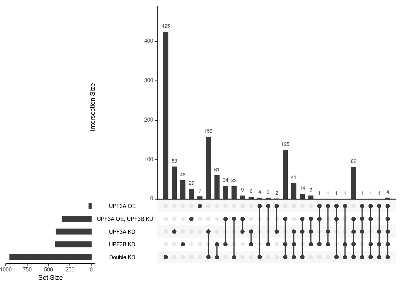
| Version | Author | Date |
|---|---|---|
| 401069b | unawaz1996 | 2023-05-04 |
UPF3B vs Controls
DEColours <- c("-1" = "#2F124B","1" = "#EA2A5F",  "0" = "#D3D5E3")
UPF3B_volc = limma_results %>%
    ggplot(aes(x = Coef.UPF3B_vs_Control,
               y = -log10(p.value.adj.UPF3B_vs_Control),
               colour = as.factor(as.character(Res.UPF3B_vs_Control)))) +
    geom_point(alpha = 0.8, size =1.5) +
    scale_colour_manual(values = DEColours) + theme_classic() +
    theme(legend.position = "none",
          axis.title.y = element_text(size = 12)) +
    geom_hline(yintercept = -log10(0.05), color = "grey60", size = 0.5, lty = "dashed") +
    #geom_hline(yintercept = -log10(limma_results %>%
     #                                  dplyr::filter(Res.UPF3B_vs_Control != 0) %>%
      #                                 use_series(p.value.adj.UPF3B_vs_Control) %>% max),
       #        color = "black") +
    labs(x = "log2 Fold Change", y = "-log10 adj p-value") +
    ggtitle("UPF3B KD vs. Control") +
  geom_vline(xintercept = c(-log2(1.5), log2(1.5)), size = 0.5, lty = "dashed", color = "grey60") + xlim(-8.5, 8.5)


#my_gg = UPF3B_volc + geom_point_interactive(aes(tooltip = gene, data_id = gene),
#    size = 1, hover_nearest = TRUE)
#girafe(ggobj = my_gg)
UPF3B_volc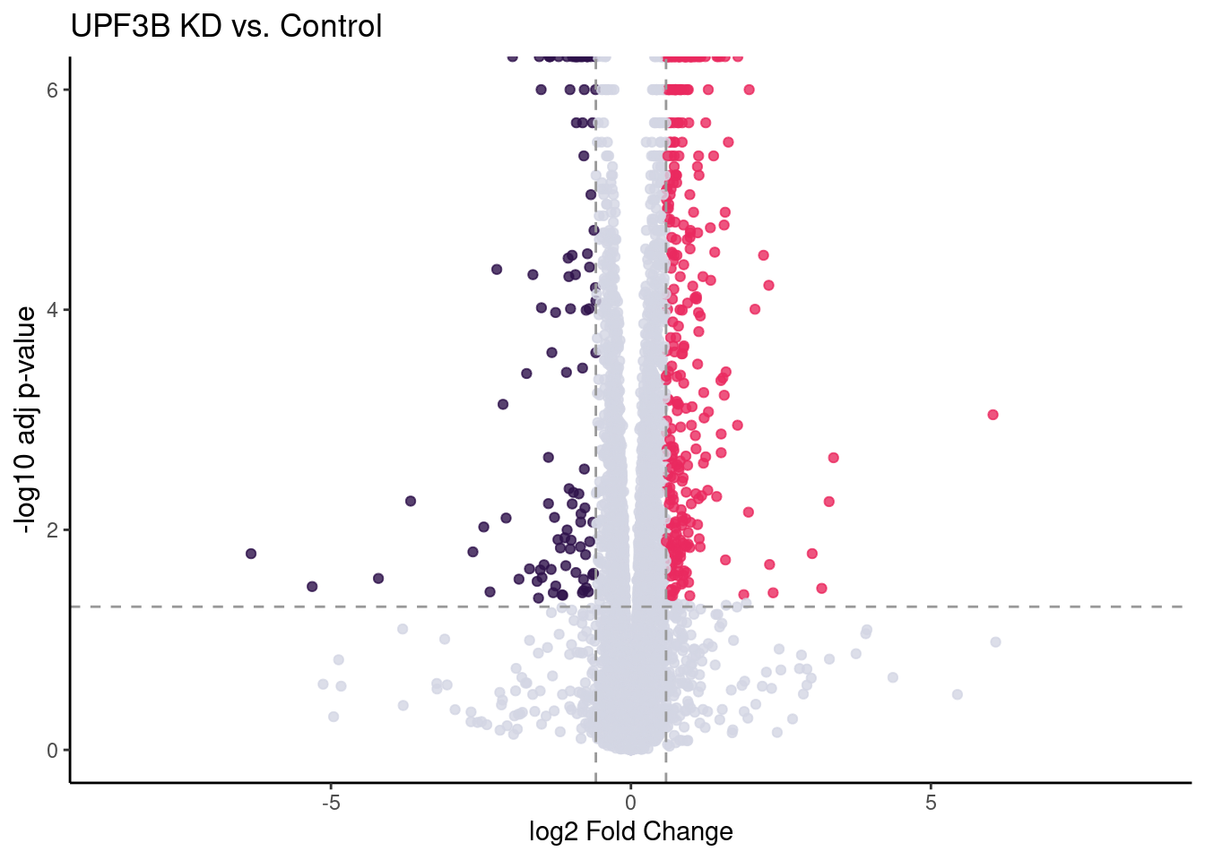
| Version | Author | Date |
|---|---|---|
| 401069b | unawaz1996 | 2023-05-04 |
## volcano plot
#ggsave(filename = "/home/neuro/Documents/NMD_analysis/Analysis/NMD-analysis/output/DEG/Thesis_figures/UPF3B_KD_volcano.svg", plot = volc,
#       units = c("in"), width = 5.97, height = 3.63)
DEGenes$UPF3B_vs_Control %>%
dplyr::select(ensembl_gene_id,gene,entrez, contains("UPF3B_vs")) %>%
dplyr::select(-contains("Res")) %>%
mutate(genename = mapIds(org.Mm.eg.db, keys=ensembl_gene_id, column="GENENAME",keytype="ENSEMBL", multiVals="first")) %>% DT::datatable(filter = 'top', extensions = c('Buttons', 'FixedColumns'), caption = "Genes significantly expressed in UPF3B KD relative to Controls", style = "auto", width = NULL, height = NULL, elementId = NULL,
options = list(scrollX = TRUE,
scrollCollapse = TRUE,
pageLength = 5, autoWidth = TRUE,
dom = 'Blfrtip',
buttons = c('copy', 'csv', 'excel', 'pdf', 'colvis'),
lengthMenu = list(c(10,25,50,-1),
c(10,25,50,"All"))))limma_results %>%
dplyr::select(ensembl_gene_id,gene,entrez, contains("UPF3B_vs")) %>%
dplyr::select(-contains("Res")) %>%
mutate(genename = mapIds(org.Mm.eg.db, keys=ensembl_gene_id, column="GENENAME",keytype="ENSEMBL", multiVals="first")) %>%
DT::datatable(filter = 'top', extensions = c('Buttons', 'FixedColumns'), caption = "Genes significantly expressed in UPF3B KD relative to Controls", style = "auto", width = NULL, height = NULL, elementId = NULL,
options = list(scrollX = TRUE,
scrollCollapse = TRUE,
pageLength = 5, autoWidth = TRUE,
dom = 'Blfrtip',
buttons = c('copy', 'csv', 'excel', 'pdf', 'colvis'),
lengthMenu = list(c(10,25,50,-1),
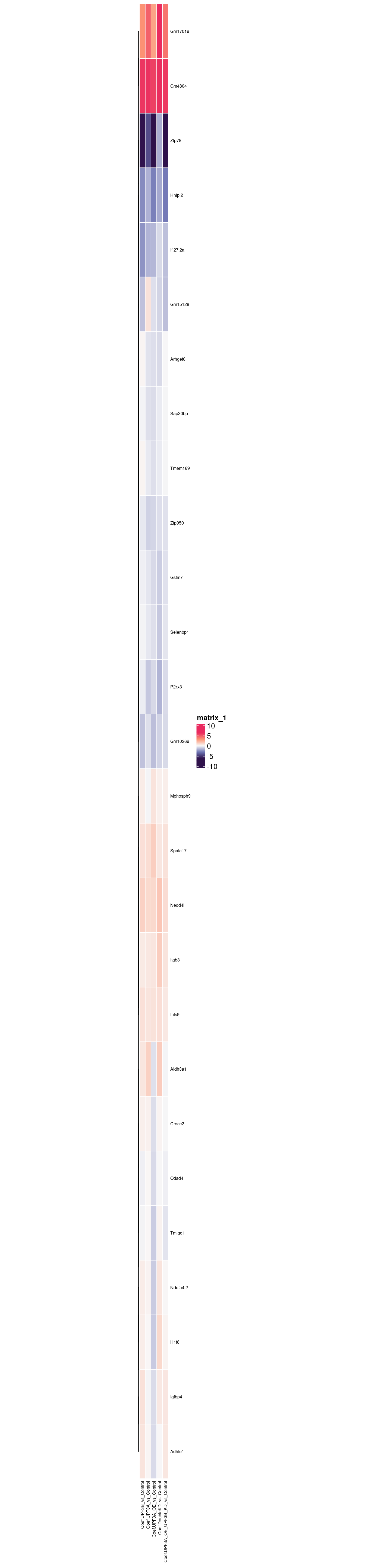
c(10,25,50,"All"))))Given that previous studies have confirmed UPF3B KD results in a decrease of efficieny of NMD resulting in an increase of upregulated genes, we are interested in seeing how the significantly expressed up-regulated genes behave in other conditions compared to controls.
In order to do this, we will create a heatmap visualisaiton.
rg <- limma_results %>%
     dplyr::filter(Res.UPF3B_vs_Control == 1) %>%
    dplyr::select(contains("Coef"), gene)  %>%
    column_to_rownames("gene") %>% max(abs(.));

limma_results %>%
    dplyr::filter(Res.UPF3B_vs_Control == 1) %>%
    dplyr::select(contains("Coef"), gene)  %>%
    column_to_rownames("gene") %>%
    pheatmap(,
        scale="none",
        cluster_cols = FALSE,
        breaks = seq(-rg, rg, length.out = 100),
        clustering_distance_rows = "euclidean",
        border_color = "white",
        treeheight_row = 0,
        fontsize = 6,
        color = colorRampPalette(c("#2F124B", "#6E74B4","#F9F9F9", "#FD9675", "#EA2A5F"))(100),
        labels_row = row.names(.),
        cellwidth = 8
    )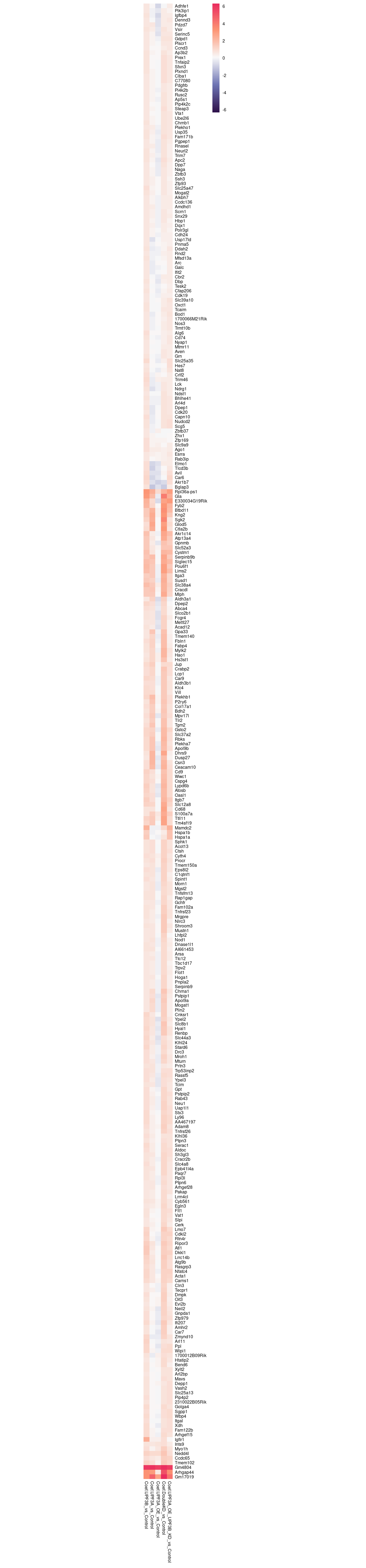
From the heatmap above, we can notice a few trends that upregulated genes in UPF3B KD have in other conditions.
Inverted expression in UPF3A OE genes
Inverted expression in UPF3A KD
These genes can be explored here:
limma_results %>%
    dplyr::filter(Res.UPF3B_vs_Control == 1) %>%
    dplyr::select(gene, contains("Coef"))  %>%
   # column_to_rownames("gene") %>%
    DT::datatable(filter = 'top', extensions = c('Buttons', 'FixedColumns'),
            options = list(scrollX = TRUE,
                           scrollCollapse = TRUE,
                           pageLength = 5, autoWidth = TRUE,
                           dom = 'Blfrtip',
                           buttons = c('copy', 'csv', 'excel', 'pdf', 'colvis'),
                           lengthMenu = list(c(10,25,50,-1),
                                             c(10,25,50,"All"))))
UPF2 levels
limma_results %>%
  dplyr::filter(ensembl_gene_id == "ENSMUSG00000038398") %>%
  column_to_rownames("ensembl_gene_id") %>%
  dplyr::select(contains("Coef.")) %>%
  melt() %>%
  ggplot(aes(x=variable, y=value)) + geom_bar(stat="identity")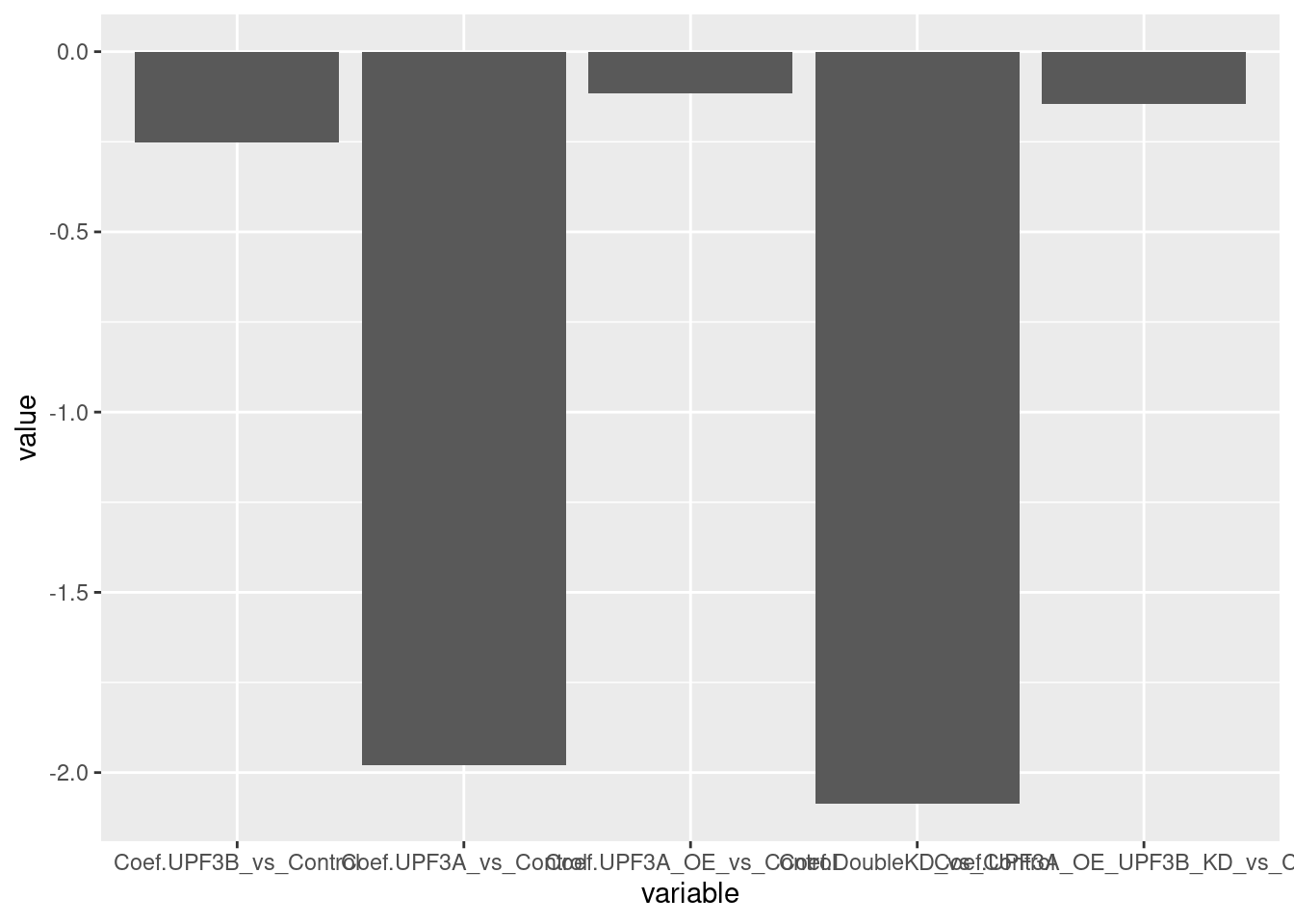
| Version | Author | Date |
|---|---|---|
| a23bb43 | unawaz1996 | 2023-05-19 |
Overlap with other significant genes
We are now also interested in seeing how all genes differentially expressed in UPF3B KD overlap with significant genes from other conditions.
Comparison with UPF3A KD significant genes
#venn(list("UPF3B KD" = DEGenes$UPF3B_vs_Control$ensembl_gene_id,
 #                      "UPF3A KD" = DEGenes$UPF3A_vs_Control$ensembl_gene_id))
x = list( "UPF3B KD" = DEGenes$UPF3B_vs_Control$ensembl_gene_id,
"UPF3A KD" = DEGenes$UPF3A_vs_Control$ensembl_gene_id,
"Double KD" = DEGenes$DoubleKD_vs_Control$ensembl_gene_id,
"UPF3A OE" = DEGenes$UPF3A_OE_vs_Control$ensembl_gene_id,
"UPF3A OE UPF3B KD" = DEGenes$UPF3A_OE_UPF3B_KD_vs_Control$ensembl_gene_id)
venn_upf3 = ggvenn(x[c(1,2)], fill_color = c("#2F124B", "#EA2A5F"),
set_name_color = "black", text_color = "white", text_size = 6,
stroke_size = 0.5, fill_alpha = 0.6)
venn_upf3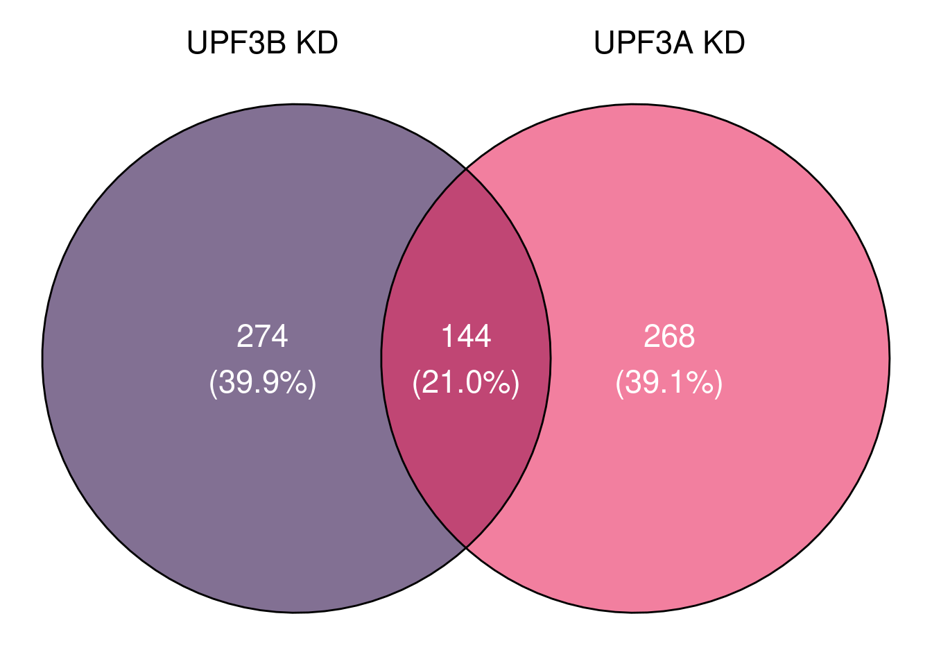
#ggsave(filename = "/home/neuro/Documents/NMD_analysis/Analysis/NMD-analysis/output/DEG/Thesis_figures/UPF3_venn.svg", plot = #venn_upf3 ,
#       units = c("in"), height = 3.30, width = 4.48)
When we compare all significant genes in UPF3B KD with UPF3A KD, we can see that there is an overlap of 144 genes.
cor_upf3KD = limma_results %>%
    dplyr::filter(Res.UPF3B_vs_Control != 0 & Res.UPF3A_vs_Control !=0) %>%
    ggscatter(., x= "Coef.UPF3B_vs_Control", y="Coef.UPF3A_vs_Control",
              cor.coef = TRUE, add = "reg.line",
              conf.int = TRUE, add.params = list(color = "blue",
                                                 fill = "lightgray")) +
    theme_bw() + ylab("UPF3A KD (log2FoldChange)") + xlab("UPF3B KD (log2FoldChange)") +
  geom_hline(yintercept = 0, size = 0.5,lty = "dashed", color = "grey60") +
  geom_vline(xintercept = 0, size = 0.5, lty = "dashed", color = "grey60")

ggsave(filename = "/home/neuro/Documents/NMD_analysis/Analysis/NMD-analysis/output/DEG/Thesis_figures/UPF3_corr.svg", plot = cor_upf3KD,
       units = c("in"), height = 3.80, width = 4.73)
When we compare the direction of gene expression in these 144 genes, we can see that there is a positive correlation (r = 0.56).
We are now interested in seeing which genes are present in each of the quadrants:
- Quadrant 1: Definied as x < 0, y > 0 where is significant genes belogning to UPF3A KD group show upregulation and genes belonging to UPF3B KD group show downregulation. A total of 14 genes belong to this group:
limma_results %>%
    dplyr::filter(Res.UPF3B_vs_Control == -1 & Res.UPF3A_vs_Control == 1) %>%
    dplyr::select(ensembl_gene_id,gene,entrez, contains(c("UPF3B_vs", "UPF3A_vs"))) %>%
    dplyr::arrange(Res.UPF3B_vs_Control) %>%
     DT::datatable(filter = 'top', extensions = c('Buttons', 'FixedColumns'),
                   caption ="Overlapping genes between UPF3B KD and UPF3A KD relative to controls in Quadrant 1 (Upregulated in UPF3A KD, downregulated in UPF3B KD)",
            options = list(scrollX = TRUE,
                           scrollCollapse = TRUE,
                           pageLength = 5, autoWidth = TRUE,
                           dom = 'Blfrtip',
                           buttons = c('copy', 'csv', 'excel', 'pdf', 'colvis'),
                           lengthMenu = list(c(10,25,50,-1),
c(10,25,50,"All"))))- Quadrant 2: Defined as x > 0, y > 0 where significant genes from both conditions show upregulation. 114 genes belong to this group.
limma_results %>%
    dplyr::filter(Res.UPF3B_vs_Control == 1 & Res.UPF3A_vs_Control ==1) %>%
    dplyr::select(ensembl_gene_id,gene,entrez, contains(c("UPF3B_vs", "UPF3A_vs"))) %>%
    dplyr::arrange(Res.UPF3B_vs_Control) %>%
    DT::datatable(filter = 'top', extensions = c('Buttons', 'FixedColumns'),
                  caption ="Overlapping genes between UPF3B KD and UPF3A KD relative to controls in Quadrant 2 (Upregulated in both conditions)",
            options = list(scrollX = TRUE,
                           scrollCollapse = TRUE,
                           pageLength = 5, autoWidth = TRUE,
                           dom = 'Blfrtip',
                           buttons = c('copy', 'csv', 'excel', 'pdf', 'colvis'),
                           lengthMenu = list(c(10,25,50,-1),
c(10,25,50,"All"))))- Quadrant 3 is defined as x < 0, y < 0 where genes in both groups show downregulation. 12 genes are in this quadrant:
limma_results %>%
    dplyr::filter(Res.UPF3B_vs_Control == -1 & Res.UPF3A_vs_Control == -1) %>%
    dplyr::select(ensembl_gene_id,gene,entrez, contains(c("UPF3B_vs", "UPF3A_vs"))) %>%
    dplyr::arrange(Res.UPF3B_vs_Control) %>%
    DT::datatable(filter = 'top', extensions = c('Buttons', 'FixedColumns'),
                  caption ="Overlapping genes between UPF3B KD and UPF3A KD relative to controls in Quadrant 3 (Downregulated in both conditions)",
            options = list(scrollX = TRUE,
                           scrollCollapse = TRUE,
                           pageLength = 5, autoWidth = TRUE,
                           dom = 'Blfrtip',
                           buttons = c('copy', 'csv', 'excel', 'pdf', 'colvis'),
                           lengthMenu = list(c(10,25,50,-1),
c(10,25,50,"All"))))- Quadrant 4 is defined as x > 0, y < 0, where significant genes belonging to UPF3B KD group are upregulated and genes belonging to UPF3A KD group are downregulated. Only 4 genes belong in this group.
limma_results %>%
dplyr::filter(Res.UPF3B_vs_Control == 1 & Res.UPF3A_vs_Control ==-1) %>%
dplyr::select(ensembl_gene_id,gene,entrez, contains(c("UPF3B_vs", "UPF3A_vs"))) %>%
dplyr::arrange(Res.UPF3B_vs_Control) %>%
DT::datatable(filter = 'top', extensions = c('Buttons', 'FixedColumns'),
caption ="Overlapping genes between UPF3B KD and UPF3A KD relative to controls in Quadrant 4 (Upregulated in UPF3B KD, downregulated in UPF3A KD)",
options = list(scrollX = TRUE,
scrollCollapse = TRUE,
pageLength = 5, autoWidth = TRUE,
dom = 'Blfrtip',
buttons = c('copy', 'csv', 'excel', 'pdf', 'colvis'),
lengthMenu = list(c(10,25,50,-1),
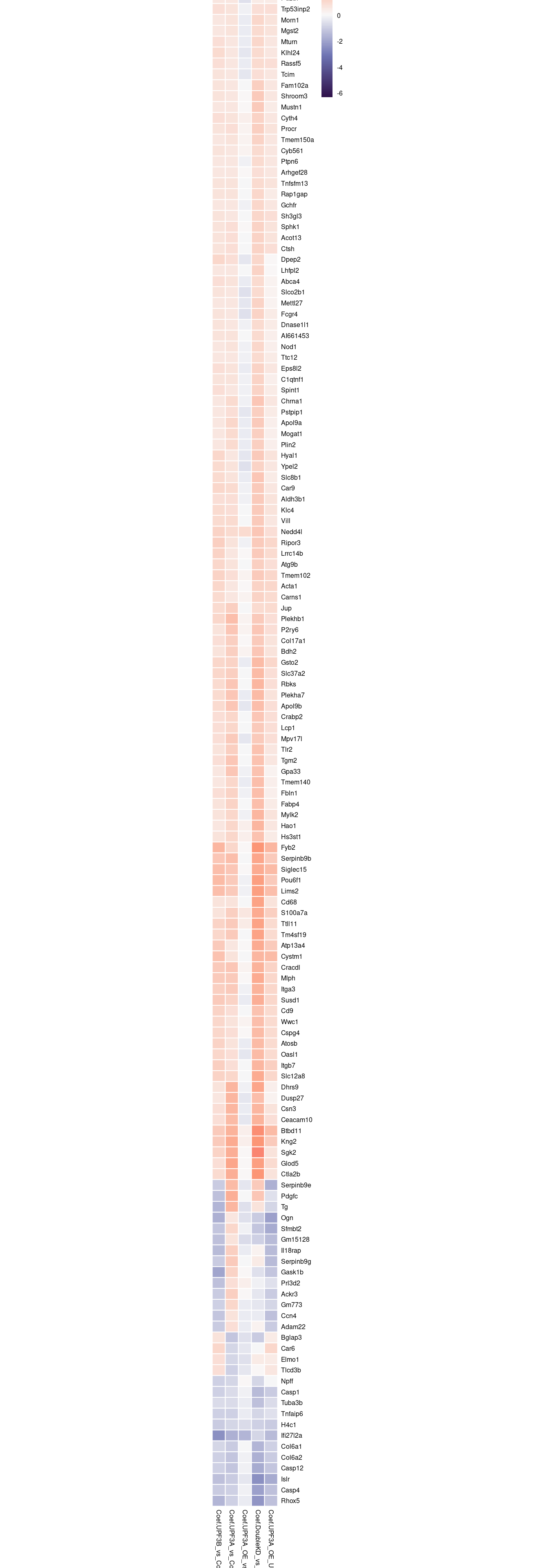
c(10,25,50,"All"))))We are also interested in seeing how the 144 overlapping genes between UPF3A and UPF3B KD behave in other conditions. To do this, we will use a heatmap visualisation again.
limma_results %>%
    dplyr::filter(Res.UPF3B_vs_Control != 0 & Res.UPF3A_vs_Control !=0) %>%
    dplyr::select(ensembl_gene_id,gene, contains(c("Coef."))) %>%
 DT::datatable(filter = 'top', extensions = c('Buttons', 'FixedColumns'),
               caption ="Overlapping genes between UPF3B KD and UPF3A KD (padj < 0.05; absolute log2FoldChange > log2(1.5)) in other comparisons)",
            options = list(scrollX = TRUE,
                           scrollCollapse = TRUE,
                           pageLength = 5, autoWidth = TRUE,
                           dom = 'Blfrtip',
                           buttons = c('copy', 'csv', 'excel', 'pdf', 'colvis'),
                           lengthMenu = list(c(10,25,50,-1),
                                             c(10,25,50,"All"))))
rg <- limma_results %>%
dplyr::filter(Res.UPF3B_vs_Control != 0 & Res.UPF3A_vs_Control !=0) %>%
dplyr::select(contains("Coef"), gene) %>%
column_to_rownames("gene") %>% max(abs(.));
limma_results %>%
dplyr::filter(Res.UPF3B_vs_Control != 0 & Res.UPF3A_vs_Control !=0) %>%
dplyr::select(contains("Coef"), gene) %>%
column_to_rownames("gene") %>%
pheatmap(,
# scale="row",
cluster_cols = FALSE,
breaks = seq(-rg, rg, length.out = 100),
clustering_distance_rows = "euclidean",
border_color = "white",
treeheight_row = 0,
cutree_rows = 2,
fontsize = 6,
color = colorRampPalette(c("#2F124B", "#6E74B4","#F9F9F9", "#FD9675", "#EA2A5F"))(100),
labels_row = row.names(.),
cellheight = 10,
cellwidth = 12
)
library(ComplexHeatmap)
library(circlize)
heatmap = limma_results %>%
dplyr::filter(Res.UPF3B_vs_Control != 0 & Res.UPF3A_vs_Control !=0) %>%
dplyr::select(contains("Coef"), gene) %>%
column_to_rownames("gene")
split = sample(letters[1:5], 144, replace = TRUE)
split = factor(split, levels = letters[1:5])
col_fun1 = colorRamp2(c(-6, 0, 6), c("#2F124B", "#F9F9F9","#EA2A5F"))
color = colorRampPalette(c("#2F124B", "#6E74B4","#F9F9F9", "#FD9675", "#EA2A5F"))(100)
circos.par(gap.after = c(2, 2, 2, 2, 10))
circos.heatmap(heatmap ,col = col_fun1, split = split, rownames.side = "outside")
circos.track(track.index = get.current.track.index(), panel.fun = function(x, y) {
if(CELL_META$sector.numeric.index == 5) { # the last sector
cn = colnames(heatmap)
n = length(cn)
circos.text(rep(CELL_META$cell.xlim[2], n) + convert_x(1, "mm"),
1:n - 0.5, cn,
cex = 0.5, adj = c(0, 0.5,0), facing = "inside")
}
}, bg.border = NA)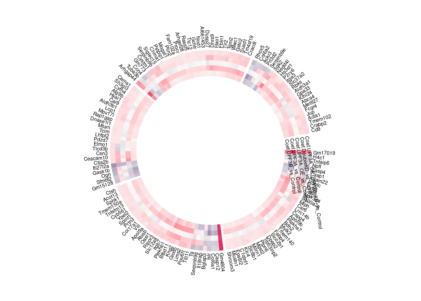
We also want to see the genes that are unique to UPF3A KD and unique to UPF3B KD and how their expression is
upf3b_uniq = limma_results %>%
    dplyr::filter(Res.UPF3B_vs_Control != 0 & Res.UPF3A_vs_Control ==0) %>%
    ggscatter(., x= "Coef.UPF3B_vs_Control", y="Coef.UPF3A_vs_Control",
              cor.coef = TRUE, add = "reg.line",
              conf.int = TRUE, add.params = list(color = "blue",
                                                 fill = "lightgray")) +
    theme_bw() + ylab("UPF3A KD (log2FoldChange)") + xlab("UPF3B KD (log2FoldChange)") +
  geom_hline(yintercept = 0, size = 0.5,lty = "dashed", color = "grey60") +
  geom_vline(xintercept = 0, size = 0.5, lty = "dashed", color = "grey60")


ggsave(filename = "/home/neuro/Documents/NMD_analysis/Analysis/NMD-analysis/output/DEG/Thesis_figures/UPF3B_corr.svg", plot = upf3b_uniq,
       units = c("in"), height = 3.80, width = 4.73)
upf3a_uniq = limma_results %>%
dplyr::filter(Res.UPF3B_vs_Control == 0 & Res.UPF3A_vs_Control !=0) %>%
ggscatter(., x= "Coef.UPF3B_vs_Control", y="Coef.UPF3A_vs_Control",
cor.coef = TRUE, add = "reg.line",
conf.int = TRUE, add.params = list(color = "blue",
fill = "lightgray")) +
theme_bw() + ylab("UPF3A KD (log2FoldChange)") + xlab("UPF3B KD (log2FoldChange)") +
geom_hline(yintercept = 0, size = 0.5,lty = "dashed", color = "grey60") +
geom_vline(xintercept = 0, size = 0.5, lty = "dashed", color = "grey60")
ggsave(filename = "/home/neuro/Documents/NMD_analysis/Analysis/NMD-analysis/output/DEG/Thesis_figures/UPF3A_corr.svg", plot = upf3a_uniq,
units = c("in"), height = 3.80, width = 4.73)UPF3B vs Double KD
ggvenn(x[c(1,3)])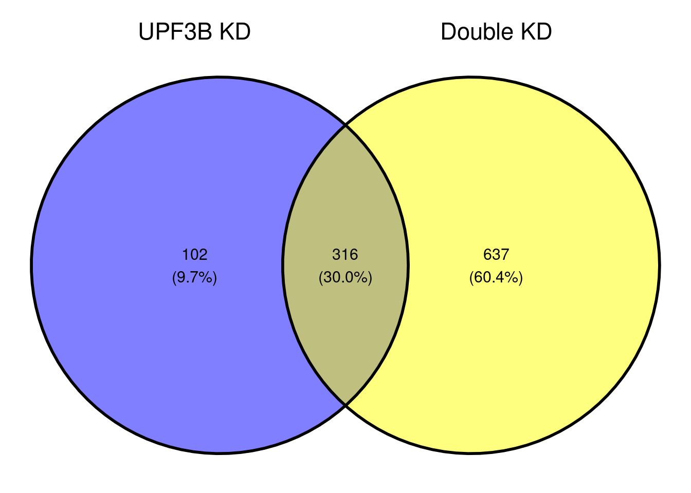
A total of 316 genes overlap betweeen the Double KDs and UPF3B KD. When we look at the correlation, we see that there is a strong positive correlation.
limma_results %>%
    dplyr::filter(Res.UPF3B_vs_Control != 0 & Res.DoubleKD_vs_Control !=0) %>%
    ggscatter(., x= "Coef.UPF3B_vs_Control", y="Coef.DoubleKD_vs_Control",
              cor.coef = TRUE, add = "reg.line",
              conf.int = TRUE, add.params = list(color = "blue",
                                                 fill = "lightgray")) +
theme_bw() 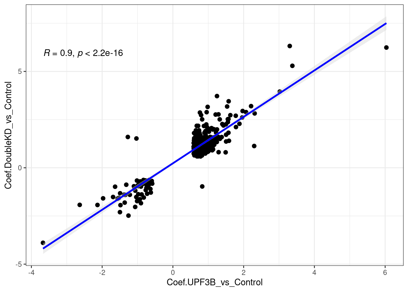
- Quadrant 1: Defined as x < 0, y > 0 where is significant genes belonging to Double KD group show upregulation and genes belonging to UPF3B KD group show downregulation. A total of 2 genes belong to this group:
limma_results %>%
    dplyr::filter(Res.UPF3B_vs_Control == -1 & Res.DoubleKD_vs_Control == 1) %>%
    dplyr::select(ensembl_gene_id,gene,entrez, contains(c("UPF3B_vs", "Double"))) %>%
    dplyr::arrange(Res.UPF3B_vs_Control) %>%
     DT::datatable(filter = 'top', extensions = c('Buttons', 'FixedColumns'),
            options = list(scrollX = TRUE,
                           scrollCollapse = TRUE,
                           pageLength = 5, autoWidth = TRUE,
                           dom = 'Blfrtip',
                           buttons = c('copy', 'csv', 'excel', 'pdf', 'colvis'),
                           lengthMenu = list(c(10,25,50,-1),
c(10,25,50,"All"))))- Quadrant 2: Defined as x > 0, y > 0 where significant genes from both conditions show upregulation. 255 genes belong to this group.
limma_results %>%
    dplyr::filter(Res.UPF3B_vs_Control == 1 & Res.DoubleKD_vs_Control ==1) %>%
    dplyr::select(ensembl_gene_id,gene,entrez, contains(c("UPF3B_vs", "DoubleKD"))) %>%
    dplyr::arrange(Res.UPF3B_vs_Control) %>%
   DT::datatable(filter = 'top', extensions = c('Buttons', 'FixedColumns'),
            options = list(scrollX = TRUE,
                           scrollCollapse = TRUE,
                           pageLength = 5, autoWidth = TRUE,
                           dom = 'Blfrtip',
                           buttons = c('copy', 'csv', 'excel', 'pdf', 'colvis'),
                           lengthMenu = list(c(10,25,50,-1),
c(10,25,50,"All"))))- Quadrant 3 is defined as x < 0, y < 0 where genes in both groups show downregulation. 58 genes are in this quadrant:
limma_results %>%
    dplyr::filter(Res.UPF3B_vs_Control == -1 & Res.DoubleKD_vs_Control == -1) %>%
    dplyr::select(ensembl_gene_id,gene,entrez, contains(c("UPF3B_vs", "DoubleKD"))) %>%
    dplyr::arrange(Res.UPF3B_vs_Control) %>%
     DT::datatable(filter = 'top', extensions = c('Buttons', 'FixedColumns'),
            options = list(scrollX = TRUE,
                           scrollCollapse = TRUE,
                           pageLength = 5, autoWidth = TRUE,
                           dom = 'Blfrtip',
                           buttons = c('copy', 'csv', 'excel', 'pdf', 'colvis'),
                           lengthMenu = list(c(10,25,50,-1),
                                             c(10,25,50,"All"))))
UPF3B vs UPF3A OE, UPF3B KD
ggvenn(x[c(1,5)])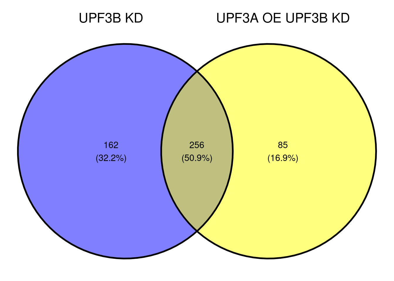
limma_results %>%
    dplyr::filter(Res.UPF3B_vs_Control != 0 & Res.UPF3A_OE_UPF3B_KD_vs_Control !=0) %>%
    ggscatter(., x= "Coef.UPF3B_vs_Control", y="Coef.UPF3A_OE_UPF3B_KD_vs_Control",
              cor.coef = TRUE, add = "reg.line",
              conf.int = TRUE, add.params = list(color = "blue",
                                                 fill = "lightgray")) +
theme_bw() 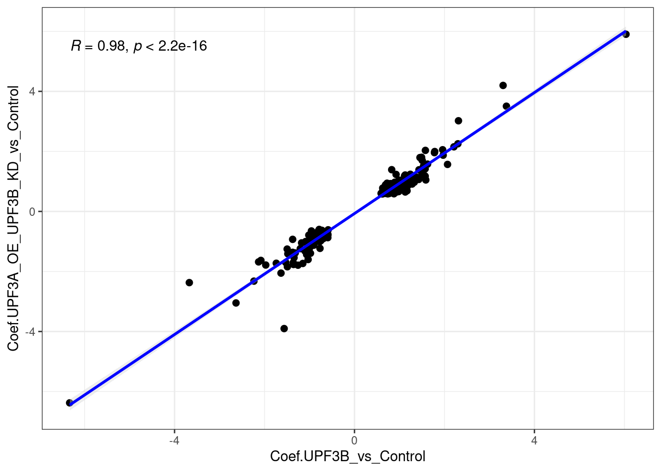
When we compare UPF3B KD with UPF3A OE in UPF3B KD cell lines, we can see there is a strong positive correlation. This correlation is very likely induced by the UPF3B KD cell line itself, and not the impact of the UPF3A OE. For interest, here are the gene in Quadrant 2 and Quadrant 3
- Quadrant 2: Defined as x > 0, y > 0 where significant genes from both conditions show upregulation. 183 genes belong to this group.
limma_results %>%
    dplyr::filter(Res.UPF3B_vs_Control == 1 & Res.UPF3A_OE_UPF3B_KD_vs_Control ==1) %>%
    dplyr::select(ensembl_gene_id,gene,entrez, contains(c("UPF3B_vs", "DoubleKD"))) %>%
    dplyr::arrange(Res.UPF3B_vs_Control) %>%
   DT::datatable(filter = 'top', extensions = c('Buttons', 'FixedColumns'),
            options = list(scrollX = TRUE,
                           scrollCollapse = TRUE,
                           pageLength = 5, autoWidth = TRUE,
                           dom = 'Blfrtip',
                           buttons = c('copy', 'csv', 'excel', 'pdf', 'colvis'),
                           lengthMenu = list(c(10,25,50,-1),
c(10,25,50,"All"))))- Quadrant 3 is defined as x < 0, y < 0 where genes in both groups show downregulation. 73 genes are in this quadrant:
limma_results %>%
    dplyr::filter(Res.UPF3B_vs_Control == -1 & Res.UPF3A_OE_UPF3B_KD_vs_Control== -1) %>%
    dplyr::select(ensembl_gene_id,gene,entrez, contains(c("UPF3B_vs", "DoubleKD"))) %>%
    dplyr::arrange(Res.UPF3B_vs_Control) %>%
     DT::datatable(filter = 'top', extensions = c('Buttons', 'FixedColumns'),
            options = list(scrollX = TRUE,
                           scrollCollapse = TRUE,
                           pageLength = 5, autoWidth = TRUE,
                           dom = 'Blfrtip',
                           buttons = c('copy', 'csv', 'excel', 'pdf', 'colvis'),
                           lengthMenu = list(c(10,25,50,-1),
                                             c(10,25,50,"All"))))
Following up from this, it would be good to see how the genes that were specific to the UPF3B KD (162 genes) and UPF3A OE, UPF3B KD (85) behave relative to the other condition.
limma_results %>%
    dplyr::filter(Res.UPF3B_vs_Control != 0 &  Res.UPF3A_OE_UPF3B_KD_vs_Control == 0 ) %>%
    ggscatter(., x= "Coef.UPF3B_vs_Control", y="Coef.UPF3A_OE_UPF3B_KD_vs_Control",
              cor.coef = TRUE, add = "reg.line",
              conf.int = TRUE, add.params = list(color = "blue",
                                                 fill = "lightgray")) +
theme_bw() 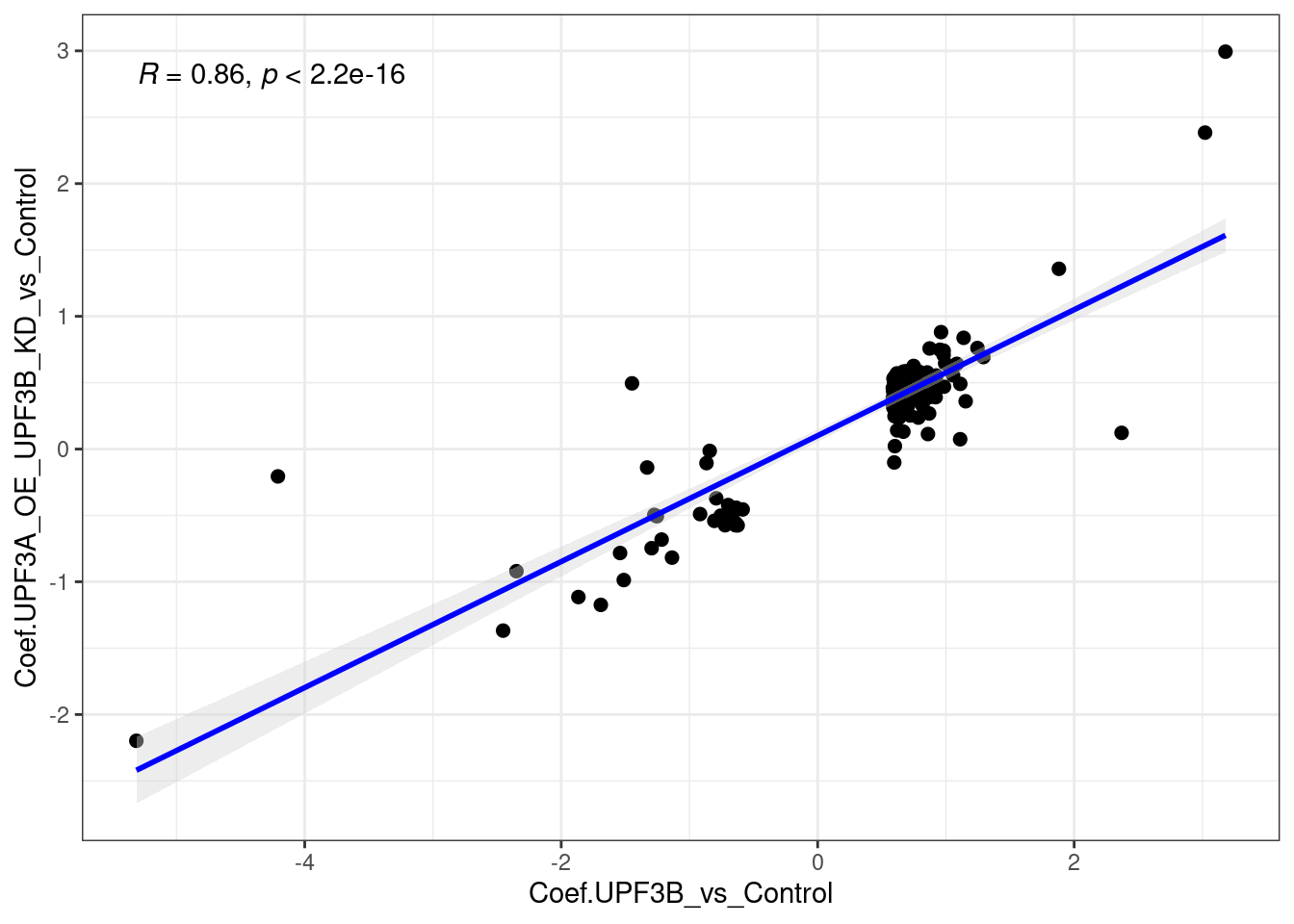
limma_results %>%
    dplyr::filter(Res.UPF3B_vs_Control ==0 &  Res.UPF3A_OE_UPF3B_KD_vs_Control != 0 ) %>%
    ggscatter(., x= "Coef.UPF3B_vs_Control", y="Coef.UPF3A_OE_UPF3B_KD_vs_Control",
              cor.coef = TRUE, add = "reg.line",
              conf.int = TRUE, add.params = list(color = "blue",
                                                 fill = "lightgray")) +
theme_bw() 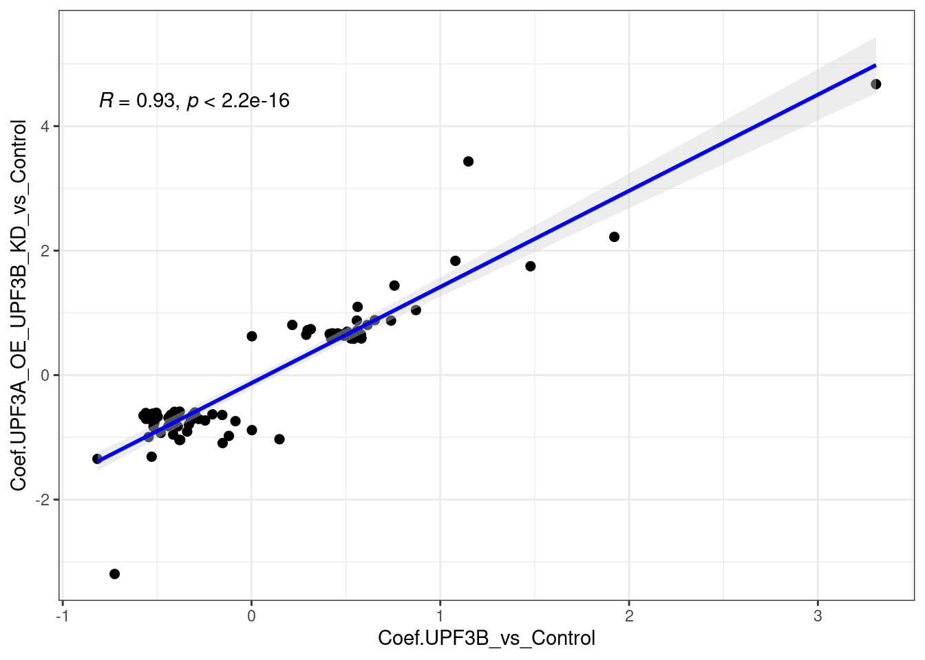
| Version | Author | Date |
|---|---|---|
| a23bb43 | unawaz1996 | 2023-05-19 |
Overall the above plots show that there is a strong positive correlation.
UPF3A
UPF3A_volc = limma_results %>%
    ggplot(aes(x = Coef.UPF3A_vs_Control,
               y = -log10(p.value.adj.UPF3A_vs_Control),
               colour = as.factor(as.character(Res.UPF3A_vs_Control)))) +
    geom_point(alpha = 0.8, size =0.8) +
    scale_colour_manual(values = DEColours) + theme_classic() +
    theme(legend.position = "none") +
    geom_hline(yintercept = -log10(0.05), color = "grey60", size = 0.5, lty = "dashed") +
    labs(x = "log2 Fold Change", y = "-log10 adj p-value") +
    ggtitle("UPF3A KD vs. Control") +
  geom_vline(xintercept = c(-log2(1.5), log2(1.5)), size = 0.5, lty = "dashed", color = "grey60") + xlim(-8.5, 8.5)


#my_gg = volc + geom_point_interactive(aes(tooltip = gene, data_id = gene),
#    size = 1, hover_nearest = TRUE)
#girafe(ggobj = my_gg)
UPF3A_volc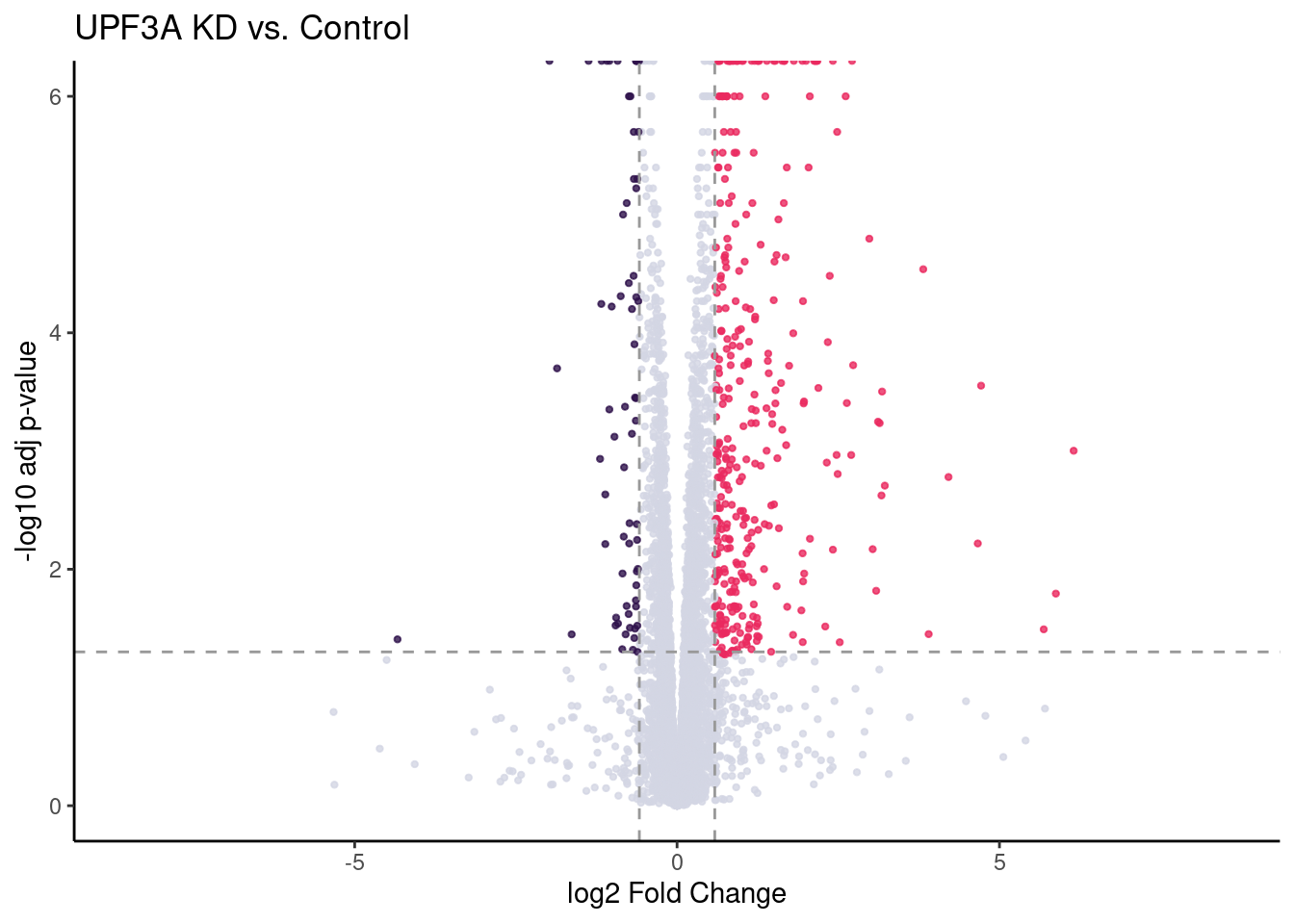
limma_results %>%
  dplyr::filter(Res.UPF3A_vs_Control != 0) %>%
    #dplyr::select(ensembl_gene_id,gene,entrez, contains("UPF3A_vs")) %>%
    mutate(genename = mapIds(org.Mm.eg.db, keys=ensembl_gene_id,  column="GENENAME",keytype="ENSEMBL", multiVals="first")) %>%     DT::datatable(filter = 'top', extensions = c('Buttons', 'FixedColumns'),
                                                                                                                                                 caption = "Genes significantly expression in UPF3A KDs relative to Controls",
            options = list(scrollX = TRUE,
                           scrollCollapse = TRUE,
                           pageLength = 5, autoWidth = TRUE,
                           dom = 'Blfrtip',
                           buttons = c('copy', 'csv', 'excel', 'pdf', 'colvis'),
                           lengthMenu = list(c(10,25,50,-1),
                                             c(10,25,50,"All"))))
UPF3A vs Double KDs
ggvenn(x[c(2,3)])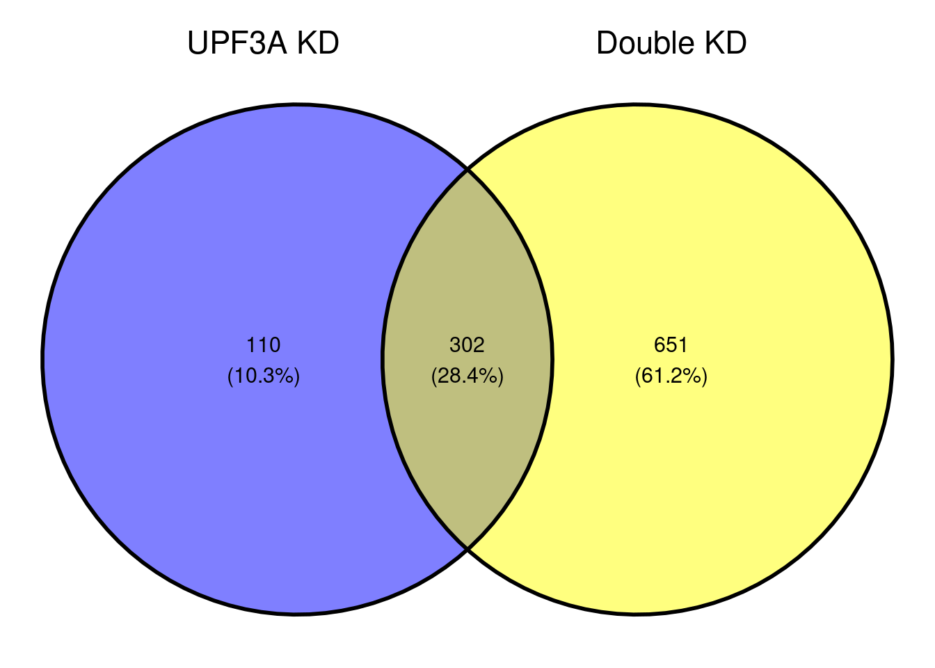
limma_results %>%
    dplyr::filter(Res.UPF3A_vs_Control != 0 & Res.DoubleKD_vs_Control !=0) %>%
    ggscatter(., x= "Coef.UPF3B_vs_Control", y="Coef.UPF3A_OE_UPF3B_KD_vs_Control",
              cor.coef = TRUE, add = "reg.line",
              conf.int = TRUE, add.params = list(color = "blue",
                                                 fill = "lightgray")) +
theme_bw() 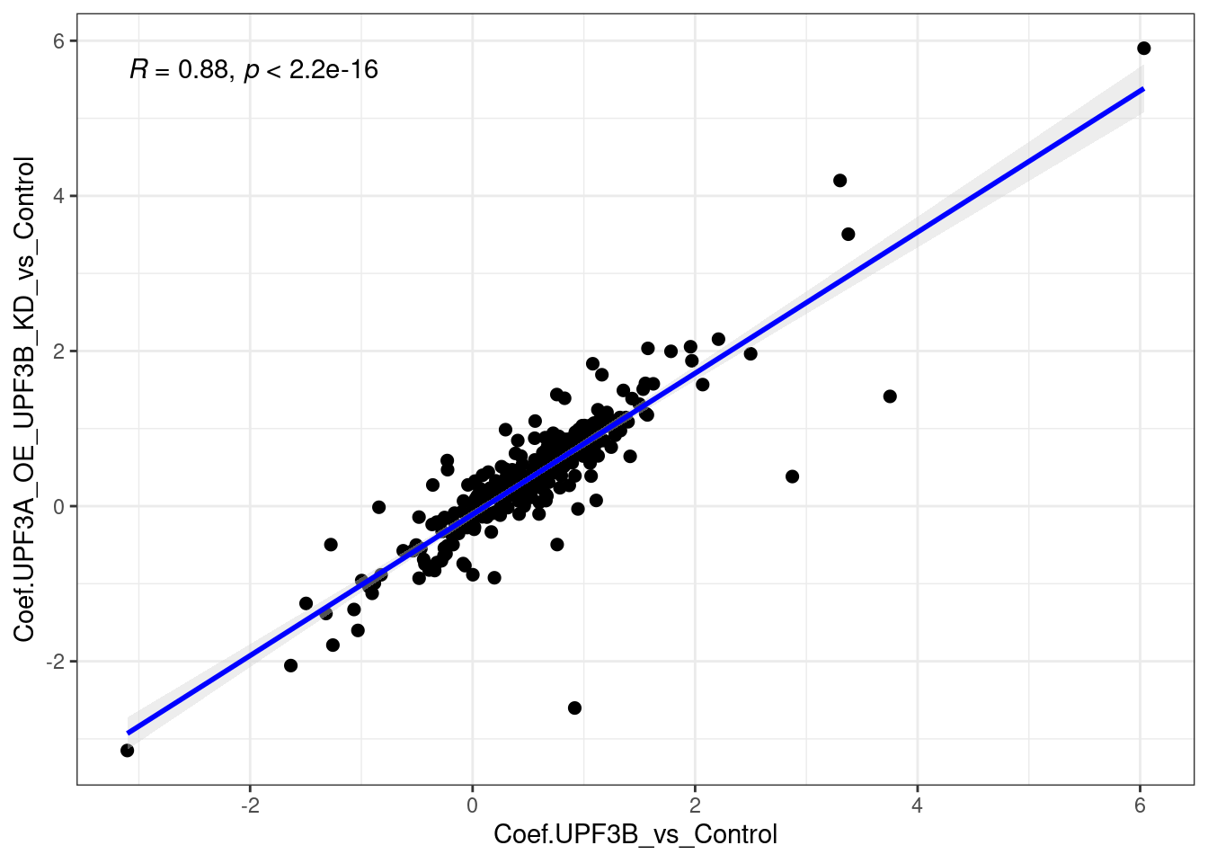
| Version | Author | Date |
|---|---|---|
| a23bb43 | unawaz1996 | 2023-05-19 |
UPF3A OE
DEGenes$UPF3A_OE_vs_Control %>%
    dplyr::select(ensembl_gene_id,gene,entrez, contains("UPF3B_vs")) %>%
    dplyr::select(-contains("Res")) %>%
    mutate(genename = mapIds(org.Mm.eg.db, keys=ensembl_gene_id,  column="GENENAME",keytype="ENSEMBL", multiVals="first")) %>%     DT::datatable(filter = 'top', extensions = c('Buttons', 'FixedColumns'), caption = "Genes significantly expressed in UPF3B KD relative to Controls", style = "auto", width = NULL, height = NULL, elementId = NULL,
            options = list(scrollX = TRUE,
                           scrollCollapse = TRUE,
                           pageLength = 5, autoWidth = TRUE,
                           dom = 'Blfrtip',
                           buttons = c('copy', 'csv', 'excel', 'pdf', 'colvis'),
                           lengthMenu = list(c(10,25,50,-1),
                                             c(10,25,50,"All"))))
rg <- limma_results %>%
dplyr::filter(Res.UPF3A_OE_vs_Control != 0) %>%
dplyr::select(contains("Coef"), gene) %>%
column_to_rownames("gene") %>% max(abs(.));
limma_results %>%
dplyr::filter(Res.UPF3A_OE_vs_Control != 0) %>%
dplyr::select(contains("Coef"), gene) %>%
column_to_rownames("gene") %>%
pheatmap(,
scale="none",
cluster_cols = FALSE,
breaks = seq(-rg, rg, length.out = 100),
clustering_distance_rows = "euclidean",
border_color = "white",
treeheight_row = 0,
fontsize = 6,
color = colorRampPalette(c("#2F124B", "#6E74B4","#F9F9F9", "#FD9675", "#EA2A5F"))(100),
labels_row = row.names(.),
cellwidth = 8
)
Heatmap of log2FCof comparisons based on genes significant in UPF3A OE compared to controls
| Version | Author | Date |
|---|---|---|
| a23bb43 | unawaz1996 | 2023-05-19 |
UPF3 dKDs
dKds_volc = limma_results %>%
    ggplot(aes(x = Coef.DoubleKD_vs_Control,
               y = -log10(p.value.adj.DoubleKD_vs_Control),
               colour = as.factor(as.character(Res.DoubleKD_vs_Control)))) +
    geom_point(alpha = 0.8, size =1.5) +
    scale_colour_manual(values = DEColours) + theme_classic() +
    theme(legend.position = "none",
          axis.title.y = element_text(size = 12)) +
    geom_hline(yintercept = -log10(0.05), color = "grey60", size = 0.5, lty = "dashed") +
    #geom_hline(yintercept = -log10(limma_results %>%
     #                                  dplyr::filter(Res.UPF3B_vs_Control != 0) %>%
      #                                 use_series(p.value.adj.UPF3B_vs_Control) %>% max),
       #        color = "black") +
    labs(x = "log2 Fold Change", y = "-log10 adj p-value") +
    ggtitle("UPF3B KD vs. Control") +
  geom_vline(xintercept = c(-log2(1.5), log2(1.5)), size = 0.5, lty = "dashed", color = "grey60") + xlim(-8.5, 8.5)
dKds_volc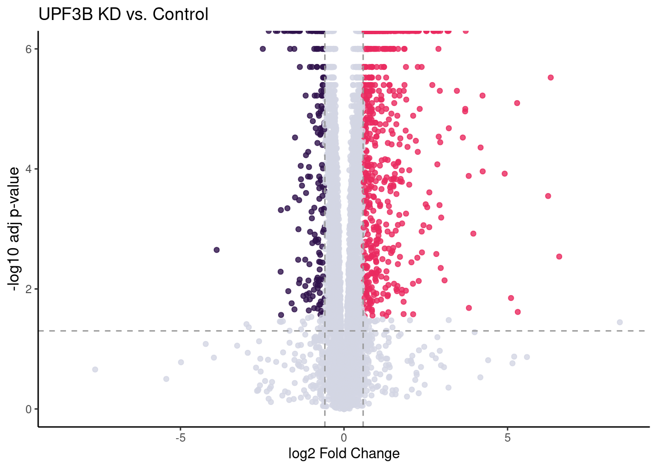
UPF3A OE
upf3a_oe_volc = limma_results %>%
    ggplot(aes(x = Coef.UPF3A_OE_vs_Control,
               y = -log10(p.value.adj.UPF3A_OE_vs_Control),
               colour = as.factor(as.character(Res.UPF3A_OE_vs_Control)))) +
    geom_point(alpha = 0.8, size =1.5) +
    scale_colour_manual(values = DEColours) + theme_classic() +
    theme(legend.position = "none",
          axis.title.y = element_text(size = 12)) +
    geom_hline(yintercept = -log10(0.05), color = "grey60", size = 0.5, lty = "dashed") +
    #geom_hline(yintercept = -log10(limma_results %>%
     #                                  dplyr::filter(Res.UPF3B_vs_Control != 0) %>%
      #                                 use_series(p.value.adj.UPF3B_vs_Control) %>% max),
       #        color = "black") +
    labs(x = "log2 Fold Change", y = "-log10 adj p-value") +
    ggtitle("UPF3B KD vs. Control") +
  geom_vline(xintercept = c(-log2(1.5), log2(1.5)), size = 0.5, lty = "dashed", color = "grey60") + xlim(-8.5, 8.5)
upf3a_oe_volc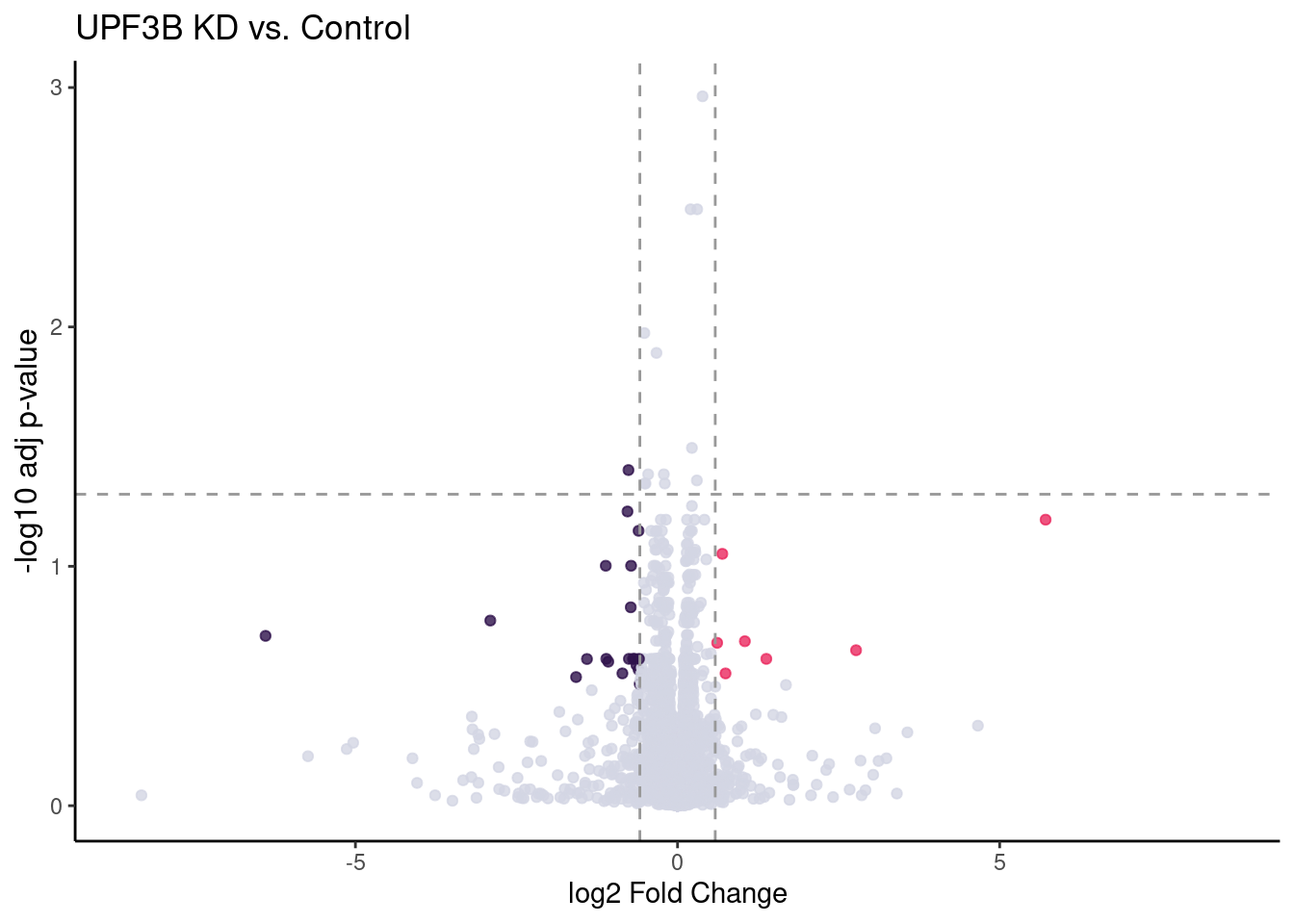
| Version | Author | Date |
|---|---|---|
| a23bb43 | unawaz1996 | 2023-05-19 |
UPF3A OE in UPF3B KD
upf3a_oe_kd_volc = limma_results %>%
    ggplot(aes(x = Coef.UPF3A_OE_UPF3B_KD_vs_Control,
               y = -log10(p.value.adj.UPF3A_OE_UPF3B_KD_vs_Control),
               colour = as.factor(as.character(Res.UPF3A_OE_UPF3B_KD_vs_Control)))) +
    geom_point(alpha = 0.8, size =1.5) +
    scale_colour_manual(values = DEColours) + theme_classic() +
    theme(legend.position = "none",
          axis.title.y = element_text(size = 12)) +
    geom_hline(yintercept = -log10(0.05), color = "grey60", size = 0.5, lty = "dashed") +
    #geom_hline(yintercept = -log10(limma_results %>%
     #                                  dplyr::filter(Res.UPF3B_vs_Control != 0) %>%
      #                                 use_series(p.value.adj.UPF3B_vs_Control) %>% max),
       #        color = "black") +
    labs(x = "log2 Fold Change", y = "-log10 adj p-value") +
    ggtitle("UPF3B KD vs. Control") +
  geom_vline(xintercept = c(-log2(1.5), log2(1.5)), size = 0.5, lty = "dashed", color = "grey60") + xlim(-8.5, 8.5)
upf3a_oe_kd_volc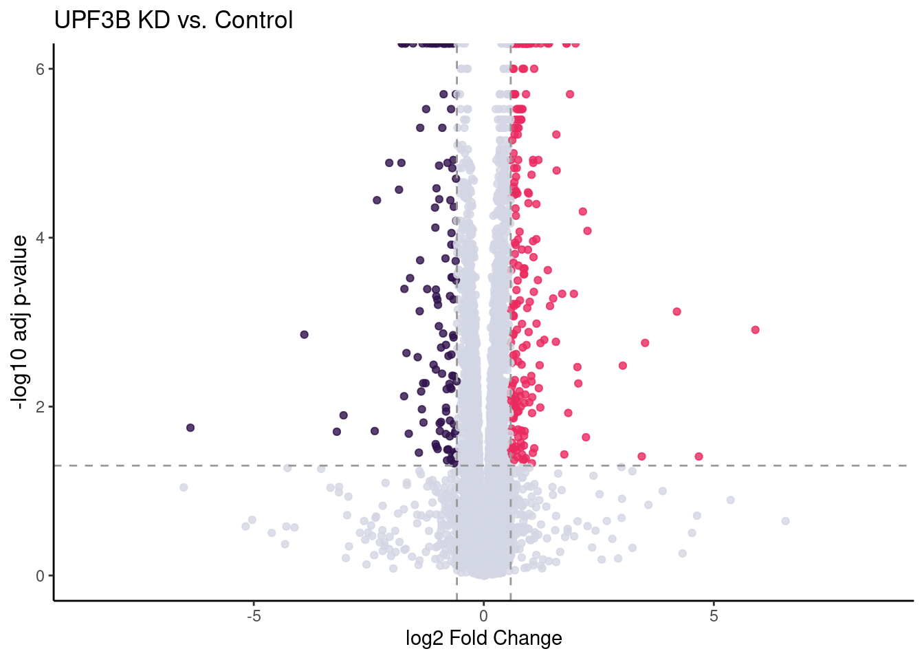
| Version | Author | Date |
|---|---|---|
| a23bb43 | unawaz1996 | 2023-05-19 |
Siginifcant genes across all conditions with respect to other conditions
rg <- limma_results %>%
     dplyr::filter(Res.UPF3B_vs_Control != 0 | Res.UPF3A_vs_Control != 0 |
                Res.DoubleKD_vs_Control !=0 | Res.UPF3A_OE_vs_Control != 0 |
                  Res.UPF3A_OE_UPF3B_KD_vs_Control != 0) %>%
    dplyr::select(contains("Coef"), gene)  %>%
    column_to_rownames("gene") %>% max(abs(.));

limma_results %>%
  dplyr::filter(Res.UPF3B_vs_Control != 0 | Res.UPF3A_vs_Control != 0 |
                Res.DoubleKD_vs_Control !=0 | Res.UPF3A_OE_vs_Control != 0 |
                  Res.UPF3A_OE_UPF3B_KD_vs_Control != 0 ) %>%
  dplyr::select(contains("Coef"), gene)  %>%
    column_to_rownames("gene") %>%
    pheatmap(,
       # scale="row",
        cluster_cols = TRUE,
        breaks = seq(-rg, rg, length.out = 100),
        clustering_distance_rows = "euclidean",
        border_color = "white",
        treeheight_row = 0,
        cutree_rows = 2,
        fontsize = 6,
        color = colorRampPalette(c("#2F124B", "#6E74B4","#F9F9F9", "#FD9675", "#EA2A5F"))(100),
        labels_row = row.names(.)
    )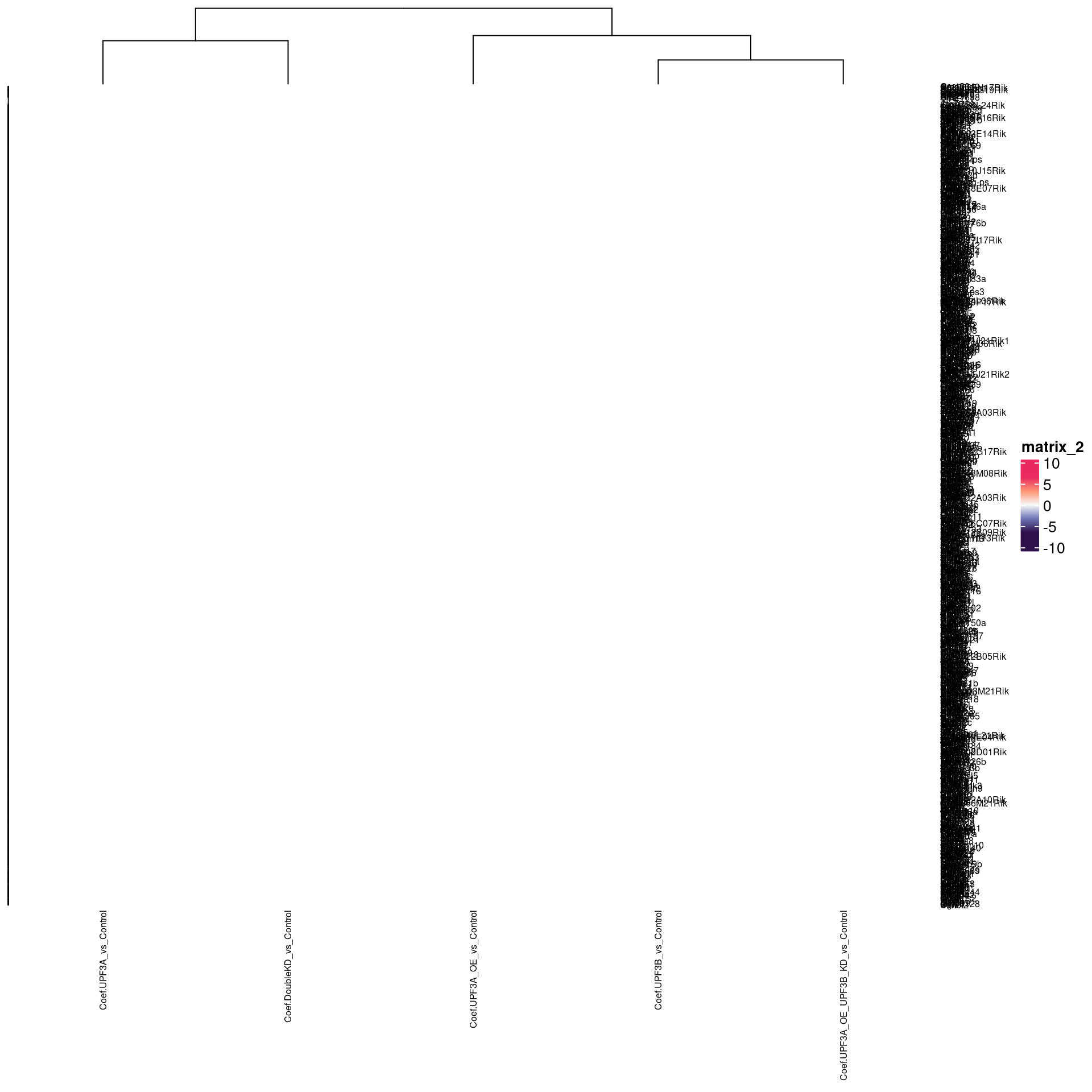
Heatmap of log fold changes across different comparisons for genes that were significant in at least 1 pairwise comparison aganst controls
| Version | Author | Date |
|---|---|---|
| a23bb43 | unawaz1996 | 2023-05-19 |
Data export
save(DEGenes, file=here::here("output/DEG-list.Rda"))
save(limma_results, file=here::here("output/DEG-limma-results.Rda"))
save(results, fit,y,v,contrasts, design, contrasts,  file = here::here("output/limma-matrices.Rda"))
sessionInfo()R version 4.2.2 Patched (2022-11-10 r83330)
Platform: x86_64-pc-linux-gnu (64-bit)
Running under: Ubuntu 22.04.2 LTS
Matrix products: default
BLAS: /usr/lib/x86_64-linux-gnu/blas/libblas.so.3.10.0
LAPACK: /usr/lib/x86_64-linux-gnu/lapack/liblapack.so.3.10.0
locale:
[1] LC_CTYPE=en_AU.UTF-8 LC_NUMERIC=C
[3] LC_TIME=en_AU.UTF-8 LC_COLLATE=en_AU.UTF-8
[5] LC_MONETARY=en_AU.UTF-8 LC_MESSAGES=en_AU.UTF-8
[7] LC_PAPER=en_AU.UTF-8 LC_NAME=C
[9] LC_ADDRESS=C LC_TELEPHONE=C
[11] LC_MEASUREMENT=en_AU.UTF-8 LC_IDENTIFICATION=C
attached base packages:
[1] grid stats4 tools stats graphics grDevices utils
[8] datasets methods base
other attached packages:
[1] circlize_0.4.15 ComplexHeatmap_2.14.0
[3] ggsci_3.0.0 eulerr_7.0.0
[5] nVennR_0.2.3 IsoformSwitchAnalyzeR_2.01.04
[7] pfamAnalyzeR_0.99.0 sva_3.46.0
[9] genefilter_1.80.3 mgcv_1.8-42
[11] nlme_3.1-162 satuRn_1.6.0
[13] DEXSeq_1.44.0 BiocParallel_1.32.6
[15] ggrepel_0.9.3 pander_0.6.5
[17] msigdbr_7.5.1 cowplot_1.1.1
[19] ngsReports_2.0.3 patchwork_1.1.2
[21] VennDiagram_1.7.3 futile.logger_1.4.3
[23] UpSetR_1.4.0 fgsea_1.24.0
[25] GOplot_1.0.2 RColorBrewer_1.1-3
[27] gridExtra_2.3 ggdendro_0.1.23
[29] AnnotationHub_3.6.0 BiocFileCache_2.6.1
[31] dbplyr_2.3.2 openxlsx_4.2.5.2
[33] ggiraph_0.8.7 wasabi_1.0.1
[35] sleuth_0.30.1 DT_0.27
[37] VennDetail_1.14.0 msigdb_1.6.0
[39] GSEABase_1.60.0 graph_1.76.0
[41] annotate_1.76.0 XML_3.99-0.14
[43] pheatmap_1.0.12 ggvenn_0.1.10
[45] MetBrewer_0.2.0 ggpubr_0.6.0
[47] venn_1.11 viridis_0.6.2
[49] viridisLite_0.4.2 tximeta_1.16.1
[51] tximport_1.26.1 goseq_1.50.0
[53] geneLenDataBase_1.34.0 BiasedUrn_2.0.9
[55] org.Mm.eg.db_3.16.0 EnsDb.Mmusculus.v79_2.99.0
[57] ensembldb_2.22.0 AnnotationFilter_1.22.0
[59] GenomicFeatures_1.50.4 AnnotationDbi_1.60.2
[61] biomaRt_2.54.1 edgeR_3.40.2
[63] limma_3.54.2 DESeq2_1.38.3
[65] SummarizedExperiment_1.28.0 Biobase_2.58.0
[67] MatrixGenerics_1.10.0 matrixStats_0.63.0
[69] GenomicRanges_1.50.2 GenomeInfoDb_1.34.9
[71] IRanges_2.32.0 S4Vectors_0.36.2
[73] BiocGenerics_0.44.0 corrplot_0.92
[75] lubridate_1.9.2 forcats_1.0.0
[77] purrr_1.0.1 readr_2.1.4
[79] tidyverse_2.0.0 stringr_1.5.0
[81] tidyr_1.3.0 scales_1.2.1
[83] data.table_1.14.8 readxl_1.4.2
[85] tibble_3.2.1 magrittr_2.0.3
[87] reshape2_1.4.4 ggplot2_3.4.2
[89] dplyr_1.1.1 workflowr_1.7.0
loaded via a namespace (and not attached):
[1] rappdirs_0.3.3 rtracklayer_1.58.0
[3] ragg_1.2.5 bit64_4.0.5
[5] knitr_1.42 DelayedArray_0.24.0
[7] hwriter_1.3.2.1 doParallel_1.0.17
[9] KEGGREST_1.38.0 RCurl_1.98-1.12
[11] generics_0.1.3 callr_3.7.3
[13] lambda.r_1.2.4 RSQLite_2.3.1
[15] bit_4.0.5 tzdb_0.3.0
[17] xml2_1.3.3 httpuv_1.6.9
[19] xfun_0.38 hms_1.1.3
[21] jquerylib_0.1.4 babelgene_22.9
[23] evaluate_0.20 promises_1.2.0.1
[25] fansi_1.0.4 restfulr_0.0.15
[27] progress_1.2.2 DBI_1.1.3
[29] geneplotter_1.76.0 htmlwidgets_1.6.2
[31] ellipsis_0.3.2 crosstalk_1.2.0
[33] backports_1.4.1 locfdr_1.1-8
[35] vctrs_0.6.2 here_1.0.1
[37] abind_1.4-5 cachem_1.0.7
[39] withr_2.5.0 BSgenome_1.66.3
[41] vroom_1.6.1 GenomicAlignments_1.34.1
[43] prettyunits_1.1.1 cluster_2.1.4
[45] svglite_2.1.1 lazyeval_0.2.2
[47] crayon_1.5.2 labeling_0.4.2
[49] pkgconfig_2.0.3 ProtGenerics_1.30.0
[51] rlang_1.1.1 lifecycle_1.0.3
[53] filelock_1.0.2 cellranger_1.1.0
[55] rprojroot_2.0.3 Matrix_1.5-3
[57] carData_3.0-5 boot_1.3-28.1
[59] Rhdf5lib_1.20.0 zoo_1.8-11
[61] GlobalOptions_0.1.2 whisker_0.4.1
[63] processx_3.8.0 png_0.1-8
[65] rjson_0.2.21 bitops_1.0-7
[67] getPass_0.2-2 rhdf5filters_1.10.1
[69] Biostrings_2.66.0 blob_1.2.4
[71] shape_1.4.6 rstatix_0.7.2
[73] ggsignif_0.6.4 memoise_2.0.1
[75] plyr_1.8.8 zlibbioc_1.44.0
[77] compiler_4.2.2 BiocIO_1.8.0
[79] clue_0.3-64 Rsamtools_2.14.0
[81] cli_3.6.1 XVector_0.38.0
[83] pbapply_1.7-0 ps_1.7.4
[85] formatR_1.14 MASS_7.3-58.3
[87] tidyselect_1.2.0 stringi_1.7.12
[89] textshaping_0.3.6 highr_0.10
[91] yaml_2.3.7 locfit_1.5-9.7
[93] sass_0.4.5 fastmatch_1.1-3
[95] timechange_0.2.0 parallel_4.2.2
[97] rstudioapi_0.14 uuid_1.1-0
[99] foreach_1.5.2 git2r_0.31.0
[101] farver_2.1.1 digest_0.6.31
[103] BiocManager_1.30.20 shiny_1.7.4
[105] Rcpp_1.0.10 car_3.1-2
[107] broom_1.0.4 BiocVersion_3.16.0
[109] later_1.3.0 httr_1.4.5
[111] colorspace_2.1-0 fs_1.6.1
[113] splines_4.2.2 statmod_1.5.0
[115] plotly_4.10.1 systemfonts_1.0.4
[117] xtable_1.8-4 jsonlite_1.8.4
[119] futile.options_1.0.1 R6_2.5.1
[121] pillar_1.9.0 htmltools_0.5.5
[123] mime_0.12 glue_1.6.2
[125] fastmap_1.1.1 interactiveDisplayBase_1.36.0
[127] codetools_0.2-19 utf8_1.2.3
[129] lattice_0.20-45 bslib_0.4.2
[131] curl_5.0.0 magick_2.7.4
[133] zip_2.2.2 GO.db_3.16.0
[135] survival_3.5-5 admisc_0.31
[137] rmarkdown_2.21 munsell_0.5.0
[139] GetoptLong_1.0.5 rhdf5_2.42.0
[141] GenomeInfoDbData_1.2.9 iterators_1.0.14
[143] gtable_0.3.3