Results
Marnin Wolfe
2020-Dec-03
Last updated: 2020-12-04
Checks: 7 0
Knit directory: IITA_2020GS/
This reproducible R Markdown analysis was created with workflowr (version 1.6.2). The Checks tab describes the reproducibility checks that were applied when the results were created. The Past versions tab lists the development history.
Great! Since the R Markdown file has been committed to the Git repository, you know the exact version of the code that produced these results.
Great job! The global environment was empty. Objects defined in the global environment can affect the analysis in your R Markdown file in unknown ways. For reproduciblity it’s best to always run the code in an empty environment.
The command set.seed(20200915) was run prior to running the code in the R Markdown file. Setting a seed ensures that any results that rely on randomness, e.g. subsampling or permutations, are reproducible.
Great job! Recording the operating system, R version, and package versions is critical for reproducibility.
Nice! There were no cached chunks for this analysis, so you can be confident that you successfully produced the results during this run.
Great job! Using relative paths to the files within your workflowr project makes it easier to run your code on other machines.
Great! You are using Git for version control. Tracking code development and connecting the code version to the results is critical for reproducibility.
The results in this page were generated with repository version 79b6430. See the Past versions tab to see a history of the changes made to the R Markdown and HTML files.
Note that you need to be careful to ensure that all relevant files for the analysis have been committed to Git prior to generating the results (you can use wflow_publish or wflow_git_commit). workflowr only checks the R Markdown file, but you know if there are other scripts or data files that it depends on. Below is the status of the Git repository when the results were generated:
Ignored files:
    Ignored:    .DS_Store
    Ignored:    .Rhistory
    Ignored:    .Rproj.user/
    Ignored:    analysis/.DS_Store
    Ignored:    data/.DS_Store
    Ignored:    output/.DS_Store

Untracked files:
    Untracked:  data/GEBV_IITA_OutliersRemovedTRUE_73119.csv
    Untracked:  data/PedigreeGeneticGainCycleTime_aafolabi_01122020.csv
    Untracked:  data/iita_blupsForCrossVal_outliersRemoved_73019.rds
    Untracked:  output/DosageMatrix_IITA_2020Sep16.rds
    Untracked:  output/IITA_CleanedTrialData_2020Dec03.rds
    Untracked:  output/IITA_ExptDesignsDetected_2020Dec03.rds
    Untracked:  output/Kinship_AA_IITA_2020Sep16.rds
    Untracked:  output/Kinship_AD_IITA_2020Sep16.rds
    Untracked:  output/Kinship_A_IITA_2020Sep16.rds
    Untracked:  output/Kinship_DD_IITA2020Sep16.rds
    Untracked:  output/Kinship_D_IITA_2020Sep16.rds
    Untracked:  output/cvresults_ModelADE_chunk1.rds
    Untracked:  output/cvresults_ModelADE_chunk2.rds
    Untracked:  output/cvresults_ModelADE_chunk3.rds
    Untracked:  output/genomicPredictions_ModelADE_threestage_IITA_2020Sep21.rds
    Untracked:  output/genomicPredictions_ModelADE_twostage_IITA_2020Dec03.rds
    Untracked:  output/genomicPredictions_ModelA_threestage_IITA_2020Sep21.rds
    Untracked:  output/iita_blupsForModelTraining_twostage_asreml_2020Dec03.rds
    Untracked:  output/model_rawgetgvs_vs_year.csv
    Untracked:  output/training_data_summary.csv
    Untracked:  workflowr_log.R

Unstaged changes:
    Modified:   output/IITA_ExptDesignsDetected.rds
    Modified:   output/iita_blupsForModelTraining.rds
    Modified:   output/maxNOHAV_byStudy.csv
    Modified:   output/meanGETGVbyYear_IITA_2020Dec03.csv
Note that any generated files, e.g. HTML, png, CSS, etc., are not included in this status report because it is ok for generated content to have uncommitted changes.
These are the previous versions of the repository in which changes were made to the R Markdown (analysis/06-Results.Rmd) and HTML (docs/06-Results.html) files. If you’ve configured a remote Git repository (see ?wflow_git_remote), click on the hyperlinks in the table below to view the files as they were in that past version.
| File | Version | Author | Date | Message |
|---|---|---|---|---|
| Rmd | 79b6430 | wolfemd | 2020-12-04 | Update the analysis of rate-of-gain. Include regressions and output |
| html | 7bae38d | wolfemd | 2020-12-03 | Build site. |
| Rmd | 3cd0f44 | wolfemd | 2020-12-03 | Refresh BLUPs and GBLUPs with trials harvested so far. Include |
| html | b9bb6f8 | wolfemd | 2020-12-03 | Build site. |
| Rmd | 9718666 | wolfemd | 2020-12-03 | Refresh BLUPs and GBLUPs with trials harvested so far. Include |
| html | c97b21b | wolfemd | 2020-11-27 | Build site. |
| Rmd | 1f8cd99 | wolfemd | 2020-11-27 | Added plots of genetic gain for 4 traits. Initial analysis of GEBV vs. |
| html | d72a9ed | wolfemd | 2020-09-21 | Build site. |
| html | 9194239 | wolfemd | 2020-09-21 | Build site. |
| Rmd | 97778e7 | wolfemd | 2020-09-21 | Big update. Two types of pipeline to get BLUPs, GEBVs and GETGVs: |
Cross-validation accuracy
Conducted 5-fold x 5-reps of cross-validation (here). Three traits only, MCMDS, logFYLD, DM.
library(tidyverse)
library(magrittr)
cvresults <- readRDS(here::here("output", "cvresults_ModelA_chunk1.rds")) %>% bind_rows(readRDS(here::here("output",
    "cvresults_ModelA_chunk2.rds"))) %>% bind_rows(readRDS(here::here("output", "cvresults_ModelA_chunk3.rds"))) %>%
    mutate(Model = "A") %>% bind_rows(readRDS(here::here("output", "cvresults_ModelADE_chunk1.rds")) %>%
    bind_rows(readRDS(here::here("output", "cvresults_ModelADE_chunk2.rds"))) %>%
    bind_rows(readRDS(here::here("output", "cvresults_ModelADE_chunk3.rds"))) %>%
    mutate(Model = "ADE"))
cvresults %>% select(Trait, repeats, id, VersionOfBLUPs, accGEBV, Model) %>% ggplot(.,
aes(x = Model, y = accGEBV, fill = VersionOfBLUPs)) + geom_boxplot() + theme_bw() +
facet_wrap(~Trait, scales = "free") + scale_fill_viridis_d() + labs(title = "GEBV: Compare 3-stage and 2-stage prediction pipelines")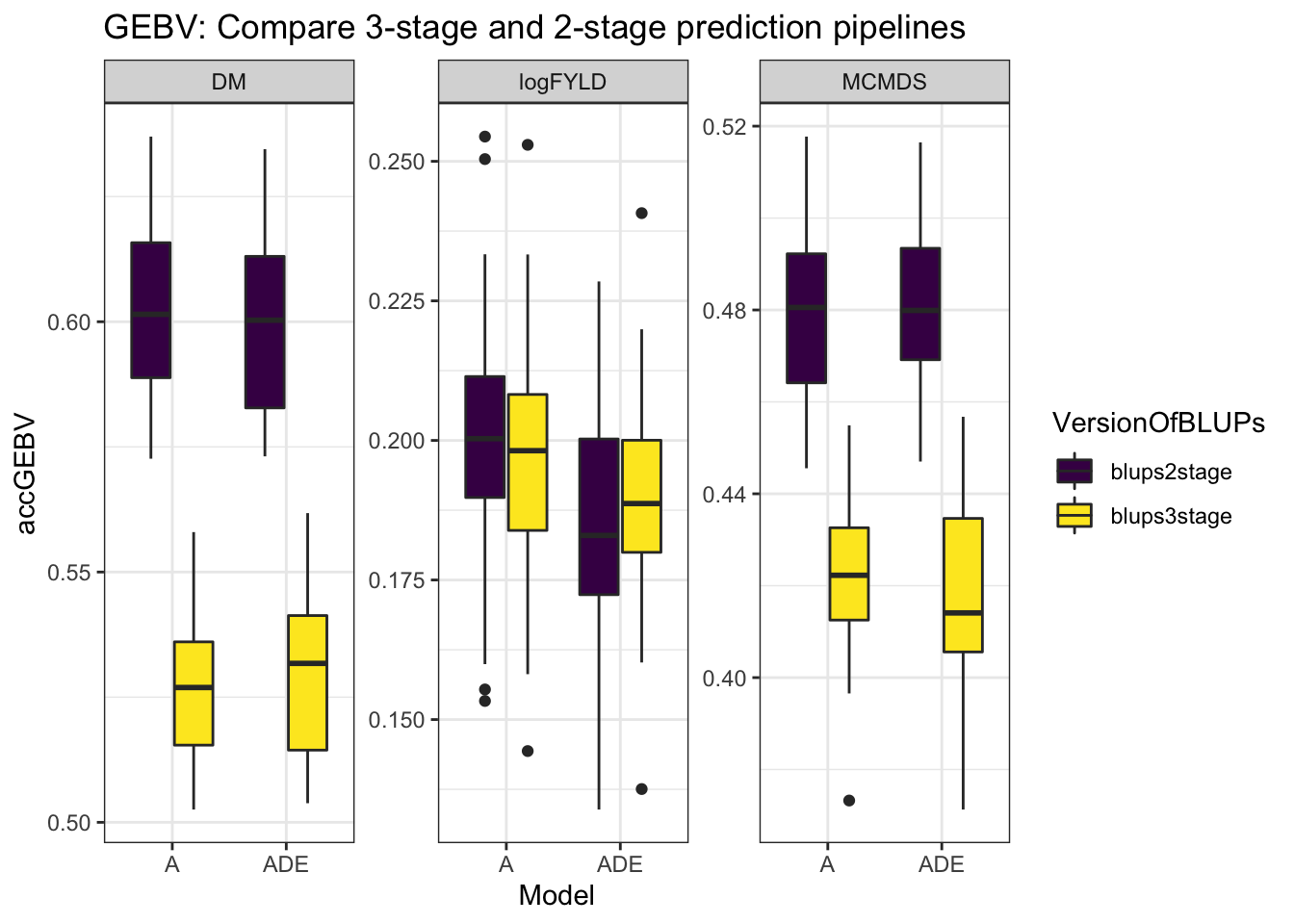
cvresults %>% select(Trait, repeats, id, VersionOfBLUPs, accGETGV, Model) %>% ggplot(.,
    aes(x = Model, y = accGETGV, fill = VersionOfBLUPs)) + geom_boxplot() + theme_bw() +
    facet_wrap(~Trait, scales = "free") + scale_fill_viridis_d() + labs(title = "GETGV: Compare 3-stage and 2-stage prediction pipelines")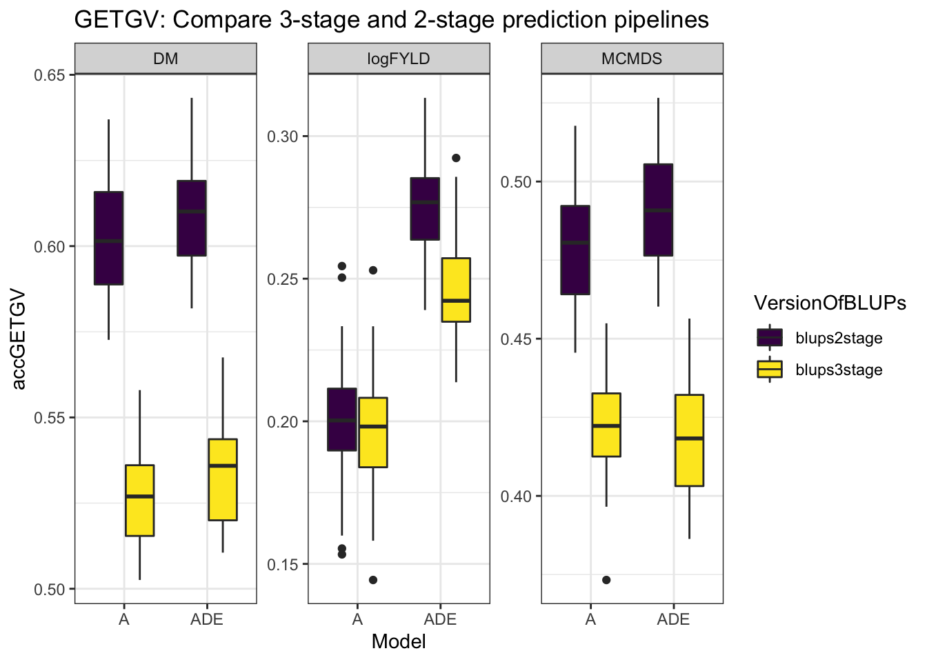
cvresults %>% select(Trait, Model, repeats, id, VersionOfBLUPs, accGEBV) %>% spread(VersionOfBLUPs,
    accGEBV) %>% mutate(diffAcc = blups2stage - blups3stage) %>% ggplot(., aes(x = Model,
    y = diffAcc, fill = Trait)) + geom_hline(yintercept = 0, color = "darkred") +
    geom_boxplot() + theme_bw() + facet_wrap(~Trait, scales = "free") + scale_fill_viridis_d() +
    labs(y = "Accuracy Difference (2-stage minus 3-stage)", title = "GEBV")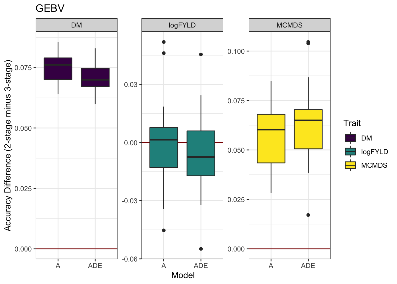
| Version | Author | Date |
|---|---|---|
| b9bb6f8 | wolfemd | 2020-12-03 |
cvresults %>% select(Trait, Model, repeats, id, VersionOfBLUPs, accGETGV) %>% spread(VersionOfBLUPs,
    accGETGV) %>% mutate(diffAcc = blups2stage - blups3stage) %>% ggplot(., aes(x = Model,
    y = diffAcc, fill = Trait)) + geom_hline(yintercept = 0, color = "darkred") +
    geom_boxplot() + theme_bw() + facet_wrap(~Trait, scales = "free") + scale_fill_viridis_d() +
    labs(y = "Accuracy Difference (2-stage minus 3-stage)", title = "GETGV")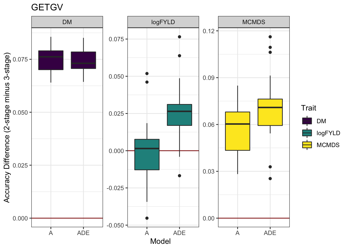
| Version | Author | Date |
|---|---|---|
| b9bb6f8 | wolfemd | 2020-12-03 |
cvresults %>% filter(VersionOfBLUPs == "blups2stage") %>% select(Trait, repeats,
    id, VersionOfBLUPs, accGETGV, Model) %>% ggplot(., aes(x = Trait, y = accGETGV,
    fill = Model)) + geom_boxplot(color = "gray60", notch = T) + theme_bw() + facet_wrap(~Trait,
    scales = "free") + scale_fill_viridis_d() + labs(title = "Compare accuracy: models A vs. ADE")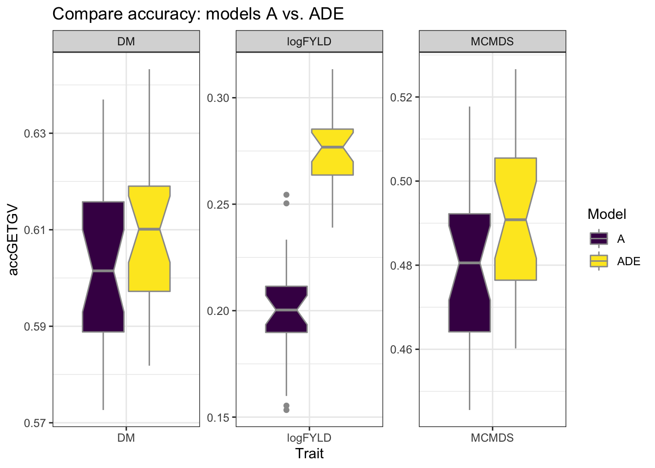
| Version | Author | Date |
|---|---|---|
| b9bb6f8 | wolfemd | 2020-12-03 |
Genetic Gain
September 2020
library(tidyverse)
library(magrittr)
iita_gebvs <- read.csv(here::here("output", "GEBV_IITA_ModelA_twostage_IITA_2020Sep21.csv"),
    stringsAsFactors = F)
traits <- c("DM", "logFYLD", "logTOPYLD", "MCMDS")
iita_gebvs %>% select(GID, GeneticGroup, any_of(traits)) %>% pivot_longer(cols = any_of(traits),
    names_to = "Trait", values_to = "GEBV") %>% group_by(Trait, GeneticGroup) %>%
    summarize(meanGEBV = mean(GEBV), stdErr = sd(GEBV)/sqrt(n()), upperSE = meanGEBV +
        stdErr, lowerSE = meanGEBV - stdErr) %>% ggplot(., aes(x = GeneticGroup,
    y = meanGEBV, fill = Trait)) + geom_bar(stat = "identity", color = "gray60",
    size = 1.25) + geom_linerange(aes(ymax = upperSE, ymin = lowerSE), color = "gray60",
    size = 1.25) + facet_wrap(~Trait, scales = "free_y", ncol = 1) + theme_bw() +
    geom_hline(yintercept = 0, size = 1.15, color = "black") + theme(axis.text.x = element_text(face = "bold",
    angle = 0, size = 12), axis.title.y = element_text(face = "bold", size = 14),
    legend.position = "none", strip.background.x = element_blank(), strip.text = element_text(face = "bold",
        size = 14)) + scale_fill_viridis_d() + labs(x = NULL, y = "Mean GEBVs")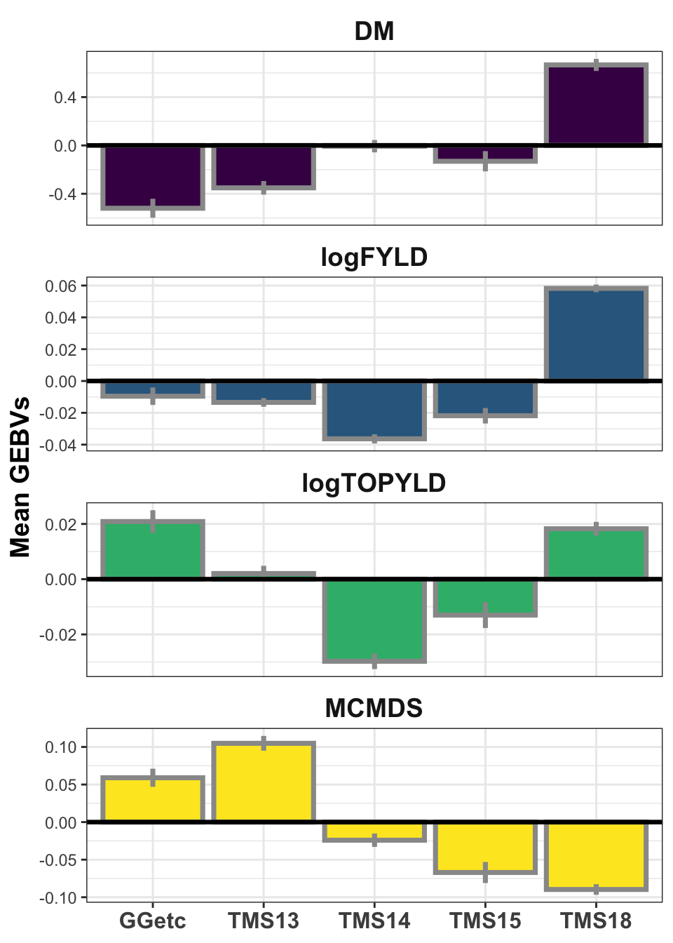
| Version | Author | Date |
|---|---|---|
| b9bb6f8 | wolfemd | 2020-12-03 |
Rate of gain
# List of trials from 2020 to Prasad and Ismail... should I download fresh data?
# dbdata<-readRDS(here::here('output','IITA_CleanedTrialData.rds'))
# trialsHarvested2019to2020<-dbdata %>% filter(studyYear>=2019) %>%
# group_by(studyYear,locationName,studyName,plantingDate,harvestDate) %>%
# summarize(Nhav=sum(!is.na(NOHAV))) trialsHarvested2019to2020 %>%
# write.csv(.,file=here::here('output','trials_uploaded_by_Nharvested_15Sep2020.csv'),
# row.names=F)
GETGV vs. “Accession Year”
Start by merging the “accession year” variable with the GETGVs.
library(tidyverse)
library(magrittr)
iita_getgvs <- read.csv(here::here("output", "GETGV_IITA_ModelADE_twostage_IITA_2020Dec03.csv"),
    stringsAsFactors = F)
traits <- c("logDYLD", "logFYLD", "MCMDS", "DM", "BCHROMO", "BRLVLS", "HI", "logTOPYLD")
# traits<-c('MCMDS','DM','PLTHT','BRNHT1','BRLVLS','HI', 'logDYLD',
# 'logFYLD','logTOPYLD','logRTNO','TCHART','LCHROMO','ACHROMO','BCHROMO')
ggcycletime <- readxl::read_xls(here::here("data", "PedigreeGeneticGainCycleTime_aafolabi_01122020.xls"))
# table(ggcycletime$Accession %in% iita_getgvs$GID) FALSE 807 Need germplasmName
# field from raw trial data to match GEBV and cycle time
dbdata <- readRDS(here::here("output", "IITA_ExptDesignsDetected_2020Dec03.rds"))
iita_getgvs %<>% left_join(dbdata %>% select(-MaxNOHAV) %>% unnest(TrialData) %>%
    distinct(germplasmName, GID)) %>% group_by(GID) %>% slice(1) %>% ungroup()
rm(dbdata)
# table(ggcycletime$Accession %in% iita_getgvs$germplasmName) FALSE TRUE 193 614

# table(ggcycletime$Year_Accession)
iita_getgvs %<>% left_join(., ggcycletime %>% rename(germplasmName = Accession) %>%
    mutate(Year_Accession = as.numeric(Year_Accession)))
iita_getgvs %<>% mutate(Year_Accession = case_when(grepl("2013_|TMS13", germplasmName) ~
    2013, grepl("TMS14", germplasmName) ~ 2014, grepl("TMS15", germplasmName) ~ 2015,
    grepl("TMS18", germplasmName) ~ 2018, !grepl("2013_|TMS13|TMS14|TMS15|TMS18",
        germplasmName) ~ Year_Accession))

write.csv(iita_getgvs, file = here::here("output", "GETGV_IITA_ModelADE_twostage_IITA_2020Dec03_withAccessionYear.csv"),
    row.names = F)
Key output is a file output/GETGV_IITA_ModelADE_twostage_IITA_2020Dec03_withAccessionYear.csv for use in downstream analyses.
What is yellow?
rm(list = ls())
library(tidyverse)
library(magrittr)
iita_getgvs <- read.csv(here::here("output", "GETGV_IITA_ModelADE_twostage_IITA_2020Dec03_withAccessionYear.csv"),
    stringsAsFactors = F)

traits <- c("logDYLD", "logFYLD", "MCMDS", "DM", "BCHROMO", "BRLVLS", "HI", "logTOPYLD")
Plot B-value and decide on a threshold for removing “yellow” clones from the analysis.
# iita_getgvs %>% ggplot(.,aes(x=TCHART,y=BCHROMO)) + geom_hex() + theme_bw() +
# facet_wrap(~GeneticGroup, nrow=1) + theme(legend.position = 'none') +
# geom_vline(xintercept = 0.5) + geom_hline(yintercept = 5) +
# labs(title='Arbitrary suggested cut-offs for `white` rooted GETGVs', subtitle =
# 'horiz. and vert. lines')
iita_getgvs %>%
ggplot(.,aes(x=BCHROMO)) + geom_histogram() +
theme_bw() + #facet_wrap(~GeneticGroup, nrow=1) +
theme(legend.position = 'none') +
geom_vline(xintercept = 1, color='darkred') + # geom_hline(yintercept = 5) +
labs(title="Histogram of GETGV for chromometer B-value",
subtitle = "Cut-offs for `white` roots == 1")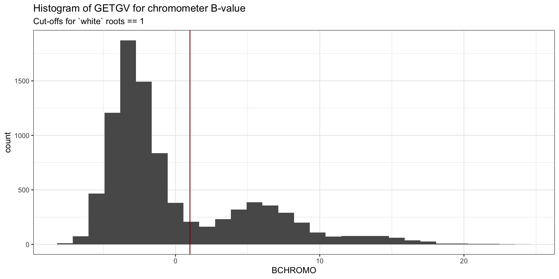
Subset years
Remove clones between 2005 and 2012.
Declare the “eras” as PreGS<2012 and GS>=2013.
iita_getgvs %<>% filter(Year_Accession > 2012 | Year_Accession < 2005)

iita_getgvs %<>% mutate(GeneticGroup = ifelse(Year_Accession >= 2013, "GS", "PreGS"))
Analysis by raw GETGVs
Number of clones for each “era” that
iita_getgvs %>% select(GeneticGroup, GID, Year_Accession, all_of(traits)) %>% count(Nclone = GeneticGroup) Nclone n
1 GS 7800
2 PreGS 449Number of white root clones (BCHROMO<=1).
iita_getgvs %>% select(GeneticGroup, GID, Year_Accession, all_of(traits)) %>% filter(BCHROMO <=
    1) %>% count(NwhiteRoot = GeneticGroup)
NwhiteRoot n
1 GS 5568
2 PreGS 346Group by Era (Genetic Group) and fit a simple linear regression for each trait, i.e. lm(GETGV ~ Year_Accession).
Fit model to “all clones” and then to “white root clones only”.
model_rawgetgvs <- iita_getgvs %>% select(GeneticGroup, GID, Year_Accession, all_of(traits)) %>%
    mutate(Dataset = "AllGermplasm") %>% bind_rows(iita_getgvs %>% select(GeneticGroup,
    GID, Year_Accession, all_of(traits)) %>% filter(BCHROMO <= 1) %>% mutate(Dataset = "WhiteRootClones")) %>%
    pivot_longer(cols = all_of(traits), names_to = "Trait", values_to = "GETGV") %>%
    nest(data = c(GID, Year_Accession, GETGV)) %>% mutate(model = map(data, ~lm(formula = "GETGV~Year_Accession",
    data = .)))
Extract the model effects, etc.
model_rawgetgvs %<>% mutate(out = map(model, ~broom::glance(.))) %>% unnest(out)
model_rawgetgvs %<>% mutate(out = map(model, ~broom::tidy(.)))
model_rawgetgvs %<>% mutate(out = map(out, ~select(., term, estimate) %>% spread(term,
    estimate))) %>% unnest(out) %>% rename(InterceptEst = `(Intercept)`, YearAccessionEst = Year_Accession) %>%
    select(Dataset, GeneticGroup, Trait, r.squared, nobs, InterceptEst, YearAccessionEst)
Basic summary of linear models
model_rawgetgvs %>% knitr::kable()| Dataset | GeneticGroup | Trait | r.squared | nobs | InterceptEst | YearAccessionEst |
|---|---|---|---|---|---|---|
| AllGermplasm | GS | logDYLD | 0.0597436 | 7800 | -32.8435514 | 0.0163021 |
| AllGermplasm | GS | logFYLD | 0.0397470 | 7800 | -34.8372928 | 0.0172871 |
| AllGermplasm | GS | MCMDS | 0.0286617 | 7800 | 72.9953447 | -0.0362284 |
| AllGermplasm | GS | DM | 0.0211352 | 7800 | -369.5705222 | 0.1834374 |
| AllGermplasm | GS | BCHROMO | 0.0101789 | 7800 | 476.2108691 | -0.2364140 |
| AllGermplasm | GS | BRLVLS | 0.0031576 | 7800 | 17.9085113 | -0.0088801 |
| AllGermplasm | GS | HI | 0.0183721 | 7800 | -5.9819828 | 0.0029696 |
| AllGermplasm | GS | logTOPYLD | 0.0067462 | 7800 | -11.6739546 | 0.0057907 |
| AllGermplasm | PreGS | logDYLD | 0.0012828 | 449 | -1.4315074 | 0.0007455 |
| AllGermplasm | PreGS | logFYLD | 0.0260293 | 449 | -8.3406627 | 0.0042546 |
| AllGermplasm | PreGS | MCMDS | 0.1126616 | 449 | 46.7030870 | -0.0234186 |
| AllGermplasm | PreGS | DM | 0.0154354 | 449 | 108.7297796 | -0.0545255 |
| AllGermplasm | PreGS | BCHROMO | 0.0162609 | 449 | -210.7971127 | 0.1052991 |
| AllGermplasm | PreGS | BRLVLS | 0.0046733 | 449 | -5.6464989 | 0.0027723 |
| AllGermplasm | PreGS | HI | 0.0068318 | 449 | -1.1127692 | 0.0005626 |
| AllGermplasm | PreGS | logTOPYLD | 0.0162925 | 449 | -5.6193029 | 0.0028573 |
| WhiteRootClones | GS | logDYLD | 0.0588583 | 5568 | -31.6705409 | 0.0157311 |
| WhiteRootClones | GS | logFYLD | 0.0531070 | 5568 | -40.9607249 | 0.0203292 |
| WhiteRootClones | GS | MCMDS | 0.0394175 | 5568 | 85.9181834 | -0.0426380 |
| WhiteRootClones | GS | DM | 0.0200139 | 5568 | -335.9238243 | 0.1670061 |
| WhiteRootClones | GS | BCHROMO | 0.0010279 | 5568 | 44.6226969 | -0.0235684 |
| WhiteRootClones | GS | BRLVLS | 0.0022178 | 5568 | -13.5887498 | 0.0067111 |
| WhiteRootClones | GS | HI | 0.0220050 | 5568 | -6.3856958 | 0.0031721 |
| WhiteRootClones | GS | logTOPYLD | 0.0169639 | 5568 | -18.5792266 | 0.0092126 |
| WhiteRootClones | PreGS | logDYLD | 0.0048734 | 346 | -2.4268634 | 0.0012559 |
| WhiteRootClones | PreGS | logFYLD | 0.0296757 | 346 | -8.2106463 | 0.0041973 |
| WhiteRootClones | PreGS | MCMDS | 0.1264779 | 346 | 45.9661526 | -0.0230526 |
| WhiteRootClones | PreGS | DM | 0.0042269 | 346 | 51.5416200 | -0.0256549 |
| WhiteRootClones | PreGS | BCHROMO | 0.0004246 | 346 | -11.4927840 | 0.0042290 |
| WhiteRootClones | PreGS | BRLVLS | 0.0002161 | 346 | 0.8557676 | -0.0005100 |
| WhiteRootClones | PreGS | HI | 0.0105153 | 346 | -1.2969781 | 0.0006570 |
| WhiteRootClones | PreGS | logTOPYLD | 0.0146826 | 346 | -4.9844269 | 0.0025395 |
Compare slope estimates between “eras”
model_rawgetgvs %>% select(Dataset, GeneticGroup, Trait, YearAccessionEst) %>% spread(GeneticGroup,
YearAccessionEst) %>% knitr::kable()| Dataset | Trait | GS | PreGS |
|---|---|---|---|
| AllGermplasm | BCHROMO | -0.2364140 | 0.1052991 |
| AllGermplasm | BRLVLS | -0.0088801 | 0.0027723 |
| AllGermplasm | DM | 0.1834374 | -0.0545255 |
| AllGermplasm | HI | 0.0029696 | 0.0005626 |
| AllGermplasm | logDYLD | 0.0163021 | 0.0007455 |
| AllGermplasm | logFYLD | 0.0172871 | 0.0042546 |
| AllGermplasm | logTOPYLD | 0.0057907 | 0.0028573 |
| AllGermplasm | MCMDS | -0.0362284 | -0.0234186 |
| WhiteRootClones | BCHROMO | -0.0235684 | 0.0042290 |
| WhiteRootClones | BRLVLS | 0.0067111 | -0.0005100 |
| WhiteRootClones | DM | 0.1670061 | -0.0256549 |
| WhiteRootClones | HI | 0.0031721 | 0.0006570 |
| WhiteRootClones | logDYLD | 0.0157311 | 0.0012559 |
| WhiteRootClones | logFYLD | 0.0203292 | 0.0041973 |
| WhiteRootClones | logTOPYLD | 0.0092126 | 0.0025395 |
| WhiteRootClones | MCMDS | -0.0426380 | -0.0230526 |
Add some summary of the raw data that went into the GETGV analyzed above.
# summarize the raw plot data
dbdata <- readRDS(here::here("output", "IITA_ExptDesignsDetected_2020Dec03.rds")) %>%
    dplyr::select(-MaxNOHAV) %>% unnest(TrialData) %>% dplyr::select(programName,
    locationName, studyYear, TrialType, studyName, CompleteBlocks, IncompleteBlocks,
    yearInLoc, trialInLocYr, repInTrial, blockInRep, observationUnitDbId, germplasmName,
    FullSampleName, GID, all_of(traits), PropNOHAV) %>% mutate(IncompleteBlocks = ifelse(IncompleteBlocks ==
    TRUE, "Yes", "No"), CompleteBlocks = ifelse(CompleteBlocks == TRUE, "Yes", "No")) %>%
    pivot_longer(cols = all_of(traits), names_to = "Trait", values_to = "Value") %>%
    filter(!is.na(Value), !is.na(GID)) %>% nest(MultiTrialTraitData = c(-Trait))

trainingdata_summary <- dbdata %>% mutate(NplotsTotal = map_dbl(MultiTrialTraitData,
    nrow), nplot = map(MultiTrialTraitData, ~count(., TrialType) %>% mutate(TrialType = paste0("Nplots_",
    TrialType)) %>% spread(TrialType, n) %>% select(any_of(paste0("Nplots_", c("CrossingBlock",
    "GeneticGain", "CET", "ExpCET", "PYT", "AYT", "UYT", "NCRP")))))) %>% unnest(nplot) %>%
    select(-MultiTrialTraitData) %>% # and add a summary of the BLUPs that result which were then later used for
# prediction
left_join(readRDS(file = here::here("output", "iita_blupsForModelTraining_twostage_asreml_2020Dec03.rds")) %>%
    filter(Trait %in% traits) %>% mutate(NclonesWithBLUPs = map_dbl(blups, nrow)) %>%
    select(Trait, NclonesWithBLUPs, Vg, Ve, H2))
Print a summary of the raw plots and resulting BLUPs that went into the GETGV .
trainingdata_summary %>% knitr::kable()| Trait | NplotsTotal | Nplots_CrossingBlock | Nplots_GeneticGain | Nplots_CET | Nplots_ExpCET | Nplots_PYT | Nplots_AYT | Nplots_UYT | Nplots_NCRP | NclonesWithBLUPs | Vg | Ve | H2 |
|---|---|---|---|---|---|---|---|---|---|---|---|---|---|
| logDYLD | 137340 | 580 | 24951 | 20345 | 799 | 26599 | 26943 | 35510 | 1613 | 26173 | 0.1561461 | 0.2208620 | 0.4141718 |
| logFYLD | 191052 | 830 | 41182 | 29673 | 1092 | 31783 | 35446 | 49013 | 2033 | 35224 | 0.3704443 | 0.2922750 | 0.5589762 |
| MCMDS | 199457 | 1246 | 11830 | 41441 | 1216 | 37252 | 40377 | 51985 | 2163 | 36292 | 0.6562184 | 0.1518826 | 0.8120500 |
| DM | 144694 | 593 | 25879 | 21044 | 800 | 28190 | 28196 | 38086 | 1618 | 26487 | 9.9466254 | 13.9393974 | 0.4164203 |
| HI | 155652 | 825 | 34146 | 24210 | 1092 | 27752 | 28606 | 37394 | 1627 | 29237 | 0.0089967 | 0.0088168 | 0.5050513 |
| logTOPYLD | 158719 | 851 | 34489 | 25058 | 1109 | 28027 | 29108 | 38448 | 1629 | 29899 | 0.1788046 | 0.2290638 | 0.4383879 |
| BRLVLS | 18551 | 275 | 1019 | 5358 | 438 | 4444 | 3260 | 3485 | 272 | 5990 | 0.4297302 | 0.5008366 | 0.4617941 |
| BCHROMO | 33611 | 242 | 3046 | 8385 | 1308 | 8753 | 5527 | 4219 | 566 | 8549 | 52.0688764 | 1.5419750 | 0.9712376 |
Write model summaries to disk: output/model_rawgetgvs_vs_year.csv.
Write training data summary to disk: output/training_data_summary.csv
write.csv(trainingdata_summary, file = here::here("output", "training_data_summary.csv"),
    row.names = F)
write.csv(model_rawgetgvs, file = here::here("output", "model_rawgetgvs_vs_year.csv"),
    row.names = F)
Plot all germplasm vs. year
iita_getgvs %>% select(GeneticGroup, GID, Year_Accession, all_of(traits)) %>% pivot_longer(cols = all_of(traits),
    names_to = "Trait", values_to = "GETGV") %>% mutate(Trait = factor(Trait, traits)) %>%
    ggplot(., aes(x = Year_Accession, y = GETGV, color = GeneticGroup)) + geom_point(size = 1.25) +
    geom_smooth(method = lm, se = TRUE, size = 1.5) + facet_wrap(~Trait, scales = "free_y",
    ncol = 2) + theme_bw() + theme(axis.text = element_text(face = "bold", angle = 0,
    size = 14), axis.title = element_text(face = "bold", size = 16), strip.background.x = element_blank(),
    strip.text = element_text(face = "bold", size = 18)) + scale_color_viridis_d() +
    labs(title = "Regression of raw GETGV vs. Year_Accession by 'era' [GS vs. PreGS]",
        subtitle = "All Germplasm")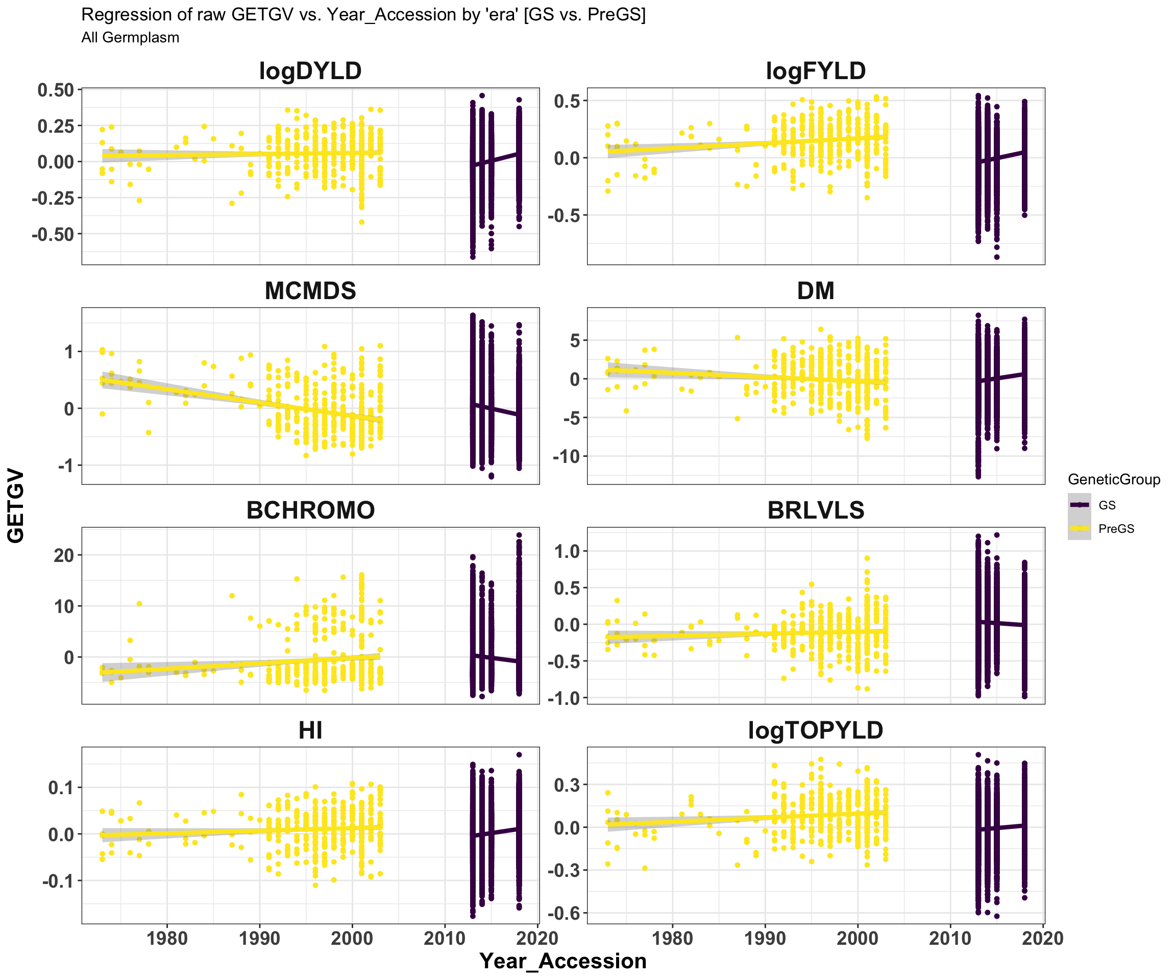
iita_getgvs %>% select(GeneticGroup, GID, Year_Accession, all_of(traits)) %>% filter(BCHROMO <=
    1) %>% pivot_longer(cols = all_of(traits), names_to = "Trait", values_to = "GETGV") %>%
    mutate(Trait = factor(Trait, traits)) %>% ggplot(., aes(x = Year_Accession, y = GETGV,
    color = GeneticGroup)) + geom_point(size = 1.25) + geom_smooth(method = lm, se = TRUE,
    size = 1.5) + facet_wrap(~Trait, scales = "free_y", ncol = 2) + theme_bw() +
    theme(axis.text = element_text(face = "bold", angle = 0, size = 14), axis.title = element_text(face = "bold",
        size = 16), strip.background.x = element_blank(), strip.text = element_text(face = "bold",
        size = 18)) + scale_color_viridis_d() + labs(title = "Regression of raw GETGV vs. Year_Accession by 'era' [GS vs. PreGS]",
    subtitle = "White Root Germplasm (BCHROMO<=1)")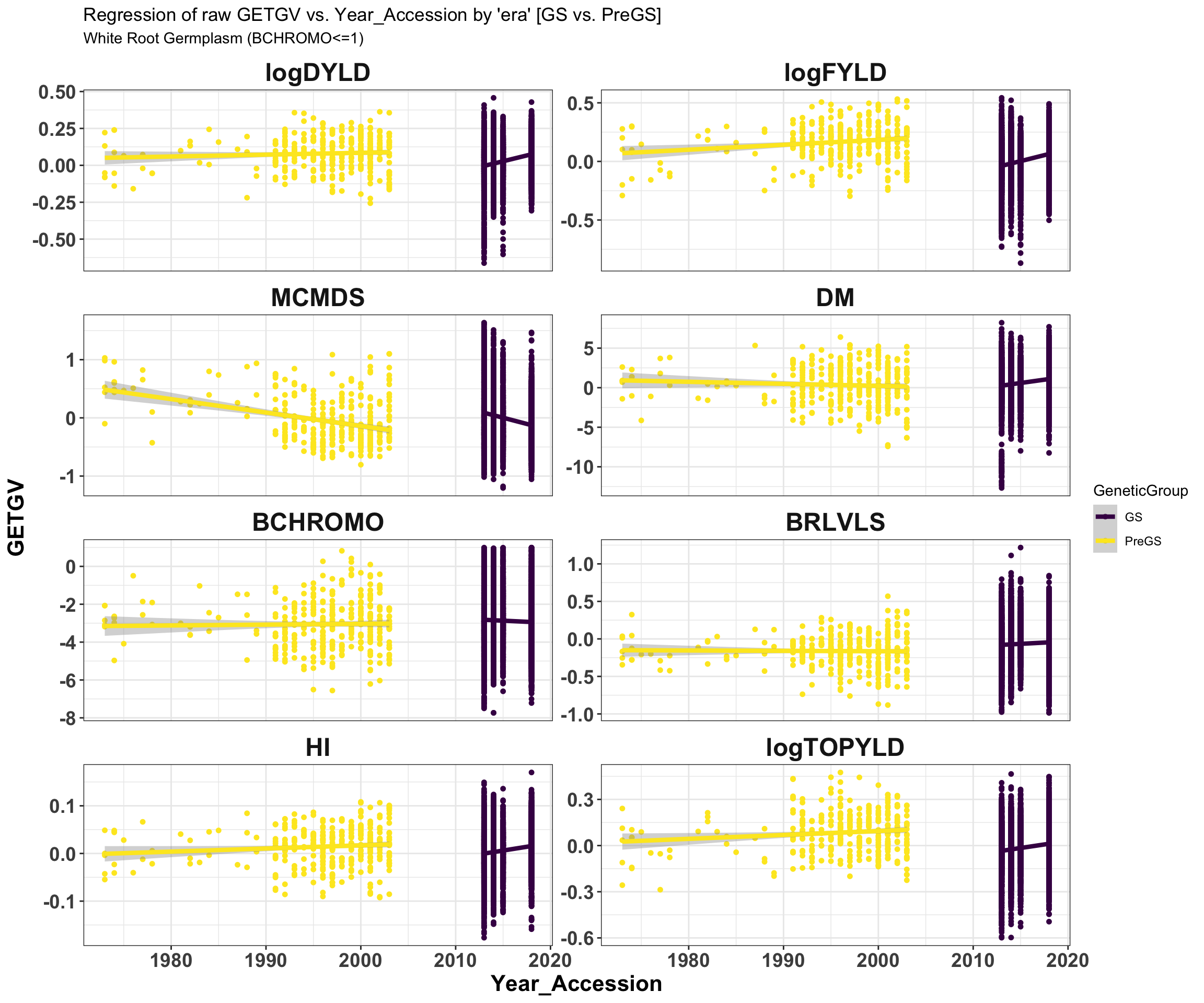
Analysis by mean GETGV-by-Year
I recommend using the analysis and maybe also the plots above.
For completeness, below is an analysis and plots using the meanGETGV-by-year.
Compute mean and std. error by Dataset (“all germplasm” vs. “white root clones only”) and GeneticGroup (“GS” vs. “PreGS”).
mean_getgvs <- iita_getgvs %>% select(GeneticGroup, GID, Year_Accession, all_of(traits)) %>%
    mutate(Dataset = "AllGermplasm") %>% bind_rows(iita_getgvs %>% select(GeneticGroup,
    GID, Year_Accession, all_of(traits)) %>% filter(BCHROMO <= 1) %>% mutate(Dataset = "WhiteRootClones")) %>%
    select(Dataset, GeneticGroup, GID, Year_Accession, all_of(traits)) %>% pivot_longer(cols = all_of(traits),
    names_to = "Trait", values_to = "GETGV") %>% group_by(Dataset, Trait, GeneticGroup,
    Year_Accession) %>% summarize(meanGETGV = mean(GETGV), Nclones = n(), stdErr = sd(GETGV)/sqrt(n()),
    upperSE = meanGETGV + stdErr, lowerSE = meanGETGV - stdErr) %>% ungroup()

write.csv(mean_getgvs, file = here::here("output", "meanGETGVbyYear_IITA_2020Dec03.csv"),
    row.names = F)
Group by Era (Genetic Group) and fit a simple linear regression for each trait, i.e. lm(GETGV ~ Year_Accession).
model_meangetgvs <- mean_getgvs %>% nest(data = c(-Dataset, -Trait, -GeneticGroup)) %>%
    mutate(model = map(data, ~lm(formula = "meanGETGV~Year_Accession", data = .)))
Extract the model effects, etc.
model_meangetgvs %<>% mutate(out = map(model, ~broom::glance(.))) %>% unnest(out) %>%
    mutate(out = map(model, ~broom::tidy(.))) %>% mutate(out = map(out, ~select(.,
    term, estimate) %>% spread(term, estimate))) %>% unnest(out) %>% rename(InterceptEst = `(Intercept)`,
    YearAccessionEst = Year_Accession) %>% select(Dataset, GeneticGroup, Trait, r.squared,
    nobs, InterceptEst, YearAccessionEst)
Basic summary of linear models
model_meangetgvs %>% knitr::kable()| Dataset | GeneticGroup | Trait | r.squared | nobs | InterceptEst | YearAccessionEst |
|---|---|---|---|---|---|---|
| AllGermplasm | GS | BCHROMO | 0.8532004 | 4 | 471.9497093 | -0.2343083 |
| AllGermplasm | PreGS | BCHROMO | 0.0429321 | 28 | -113.5633194 | 0.0566350 |
| AllGermplasm | GS | BRLVLS | 0.1280562 | 4 | 18.1115255 | -0.0089737 |
| AllGermplasm | PreGS | BRLVLS | 0.0312191 | 28 | -3.9254210 | 0.0019110 |
| AllGermplasm | GS | DM | 0.8480500 | 4 | -367.8607283 | 0.1825682 |
| AllGermplasm | PreGS | DM | 0.0026520 | 28 | 12.8247623 | -0.0064715 |
| AllGermplasm | GS | HI | 0.9169543 | 4 | -5.9505790 | 0.0029538 |
| AllGermplasm | PreGS | HI | 0.0339995 | 28 | -0.6821122 | 0.0003487 |
| AllGermplasm | GS | logDYLD | 0.9673037 | 4 | -32.7297867 | 0.0162452 |
| AllGermplasm | PreGS | logDYLD | 0.0746435 | 28 | -3.9716902 | 0.0020204 |
| AllGermplasm | GS | logFYLD | 0.7654132 | 4 | -34.9962751 | 0.0173632 |
| AllGermplasm | PreGS | logFYLD | 0.2111658 | 28 | -10.0364112 | 0.0051028 |
| AllGermplasm | GS | logTOPYLD | 0.4333553 | 4 | -11.9159076 | 0.0059094 |
| AllGermplasm | PreGS | logTOPYLD | 0.1574272 | 28 | -6.9318689 | 0.0035059 |
| AllGermplasm | GS | MCMDS | 0.7196770 | 4 | 72.2250873 | -0.0358507 |
| AllGermplasm | PreGS | MCMDS | 0.4968339 | 28 | 48.0679272 | -0.0240747 |
| WhiteRootClones | GS | BCHROMO | 0.0579712 | 4 | 39.1769308 | -0.0208431 |
| WhiteRootClones | PreGS | BCHROMO | 0.0573489 | 27 | 37.3227110 | -0.0201925 |
| WhiteRootClones | GS | BRLVLS | 0.0484472 | 4 | -15.7816767 | 0.0078091 |
| WhiteRootClones | PreGS | BRLVLS | 0.0096716 | 27 | -2.4146129 | 0.0011384 |
| WhiteRootClones | GS | DM | 0.8157617 | 4 | -334.7466632 | 0.1664016 |
| WhiteRootClones | PreGS | DM | 0.0020053 | 27 | -14.6935281 | 0.0075602 |
| WhiteRootClones | GS | HI | 0.8523860 | 4 | -6.3476943 | 0.0031529 |
| WhiteRootClones | PreGS | HI | 0.0645647 | 27 | -1.0889273 | 0.0005537 |
| WhiteRootClones | GS | logDYLD | 0.9128293 | 4 | -31.7062537 | 0.0157479 |
| WhiteRootClones | PreGS | logDYLD | 0.1270733 | 27 | -5.1261249 | 0.0026098 |
| WhiteRootClones | GS | logFYLD | 0.8254112 | 4 | -40.4750002 | 0.0200853 |
| WhiteRootClones | PreGS | logFYLD | 0.2684843 | 27 | -11.9213372 | 0.0060552 |
| WhiteRootClones | GS | logTOPYLD | 0.9356043 | 4 | -18.4227385 | 0.0091343 |
| WhiteRootClones | PreGS | logTOPYLD | 0.1687423 | 27 | -7.8116959 | 0.0039504 |
| WhiteRootClones | GS | MCMDS | 0.7636413 | 4 | 87.5299546 | -0.0434427 |
| WhiteRootClones | PreGS | MCMDS | 0.5075304 | 27 | 50.5545173 | -0.0253250 |
Compare slope estimates between “eras”
model_meangetgvs %>% select(Dataset, GeneticGroup, Trait, YearAccessionEst) %>% spread(GeneticGroup,
YearAccessionEst) %>% knitr::kable()| Dataset | Trait | GS | PreGS |
|---|---|---|---|
| AllGermplasm | BCHROMO | -0.2343083 | 0.0566350 |
| AllGermplasm | BRLVLS | -0.0089737 | 0.0019110 |
| AllGermplasm | DM | 0.1825682 | -0.0064715 |
| AllGermplasm | HI | 0.0029538 | 0.0003487 |
| AllGermplasm | logDYLD | 0.0162452 | 0.0020204 |
| AllGermplasm | logFYLD | 0.0173632 | 0.0051028 |
| AllGermplasm | logTOPYLD | 0.0059094 | 0.0035059 |
| AllGermplasm | MCMDS | -0.0358507 | -0.0240747 |
| WhiteRootClones | BCHROMO | -0.0208431 | -0.0201925 |
| WhiteRootClones | BRLVLS | 0.0078091 | 0.0011384 |
| WhiteRootClones | DM | 0.1664016 | 0.0075602 |
| WhiteRootClones | HI | 0.0031529 | 0.0005537 |
| WhiteRootClones | logDYLD | 0.0157479 | 0.0026098 |
| WhiteRootClones | logFYLD | 0.0200853 | 0.0060552 |
| WhiteRootClones | logTOPYLD | 0.0091343 | 0.0039504 |
| WhiteRootClones | MCMDS | -0.0434427 | -0.0253250 |
Save these estimates also to disk at: output/model_meangetgvs_vs_year.csv
write.csv(model_meangetgvs, file = here::here("output", "model_meangetgvs_vs_year.csv"),
    row.names = F)
Plot all germplasm vs. year
mean_getgvs %>% filter(Dataset == "AllGermplasm") %>% mutate(Trait = factor(Trait,
    traits)) %>% ggplot(., aes(x = Year_Accession, y = meanGETGV, color = GeneticGroup,
    size = Nclones)) + geom_point(size = 4) + geom_smooth(method = lm, se = TRUE) +
    geom_linerange(aes(ymax = upperSE, ymin = lowerSE), color = "gray40", size = 1) +
    facet_wrap(~Trait, scales = "free_y", ncol = 2) + theme_bw() + theme(axis.text = element_text(face = "bold",
    angle = 0, size = 14), axis.title = element_text(face = "bold", size = 16), strip.background.x = element_blank(),
    strip.text = element_text(face = "bold", size = 18)) + scale_color_viridis_d() +
    labs(title = "meanGETGV vs. Year_Accession - All Germplasm", subtitle = "Mean across all clones within Year_Accession")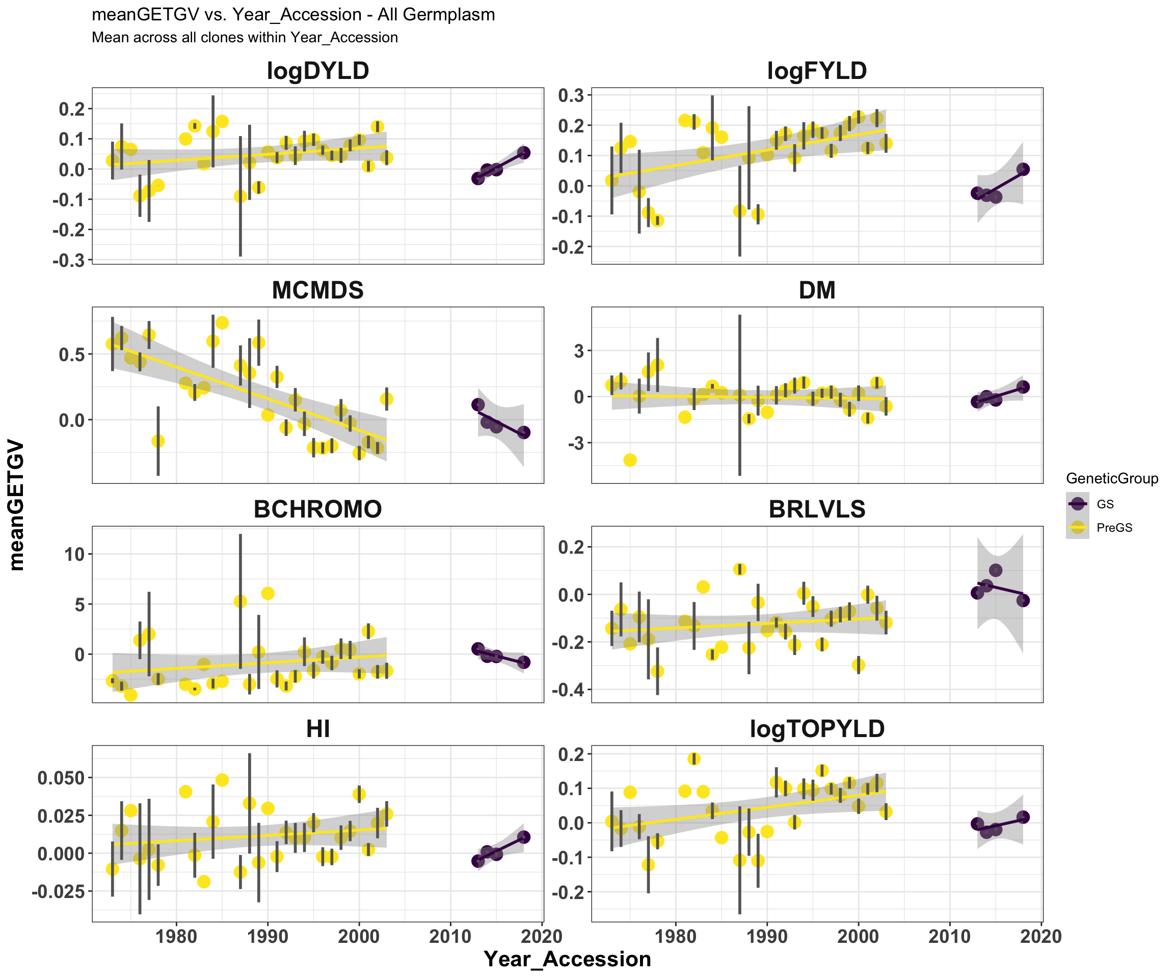
Plot “white” germplasm vs. year
mean_getgvs %>% filter(Dataset == "WhiteRootClones") %>% mutate(Trait = factor(Trait,
    traits)) %>% ggplot(., aes(x = Year_Accession, y = meanGETGV, color = GeneticGroup,
    size = Nclones)) + geom_point(size = 4) + geom_smooth(method = lm, se = TRUE) +
    geom_linerange(aes(ymax = upperSE, ymin = lowerSE), color = "gray40", size = 1) +
    facet_wrap(~Trait, scales = "free_y", ncol = 2) + theme_bw() + theme(axis.text = element_text(face = "bold",
    angle = 0, size = 14), axis.title = element_text(face = "bold", size = 16), strip.background.x = element_blank(),
    strip.text = element_text(face = "bold", size = 18)) + scale_color_viridis_d() +
    labs(title = "meanGETGV vs. Year_Accession - White rooted germplasm", subtitle = "Mean across all clones within Year_Accession")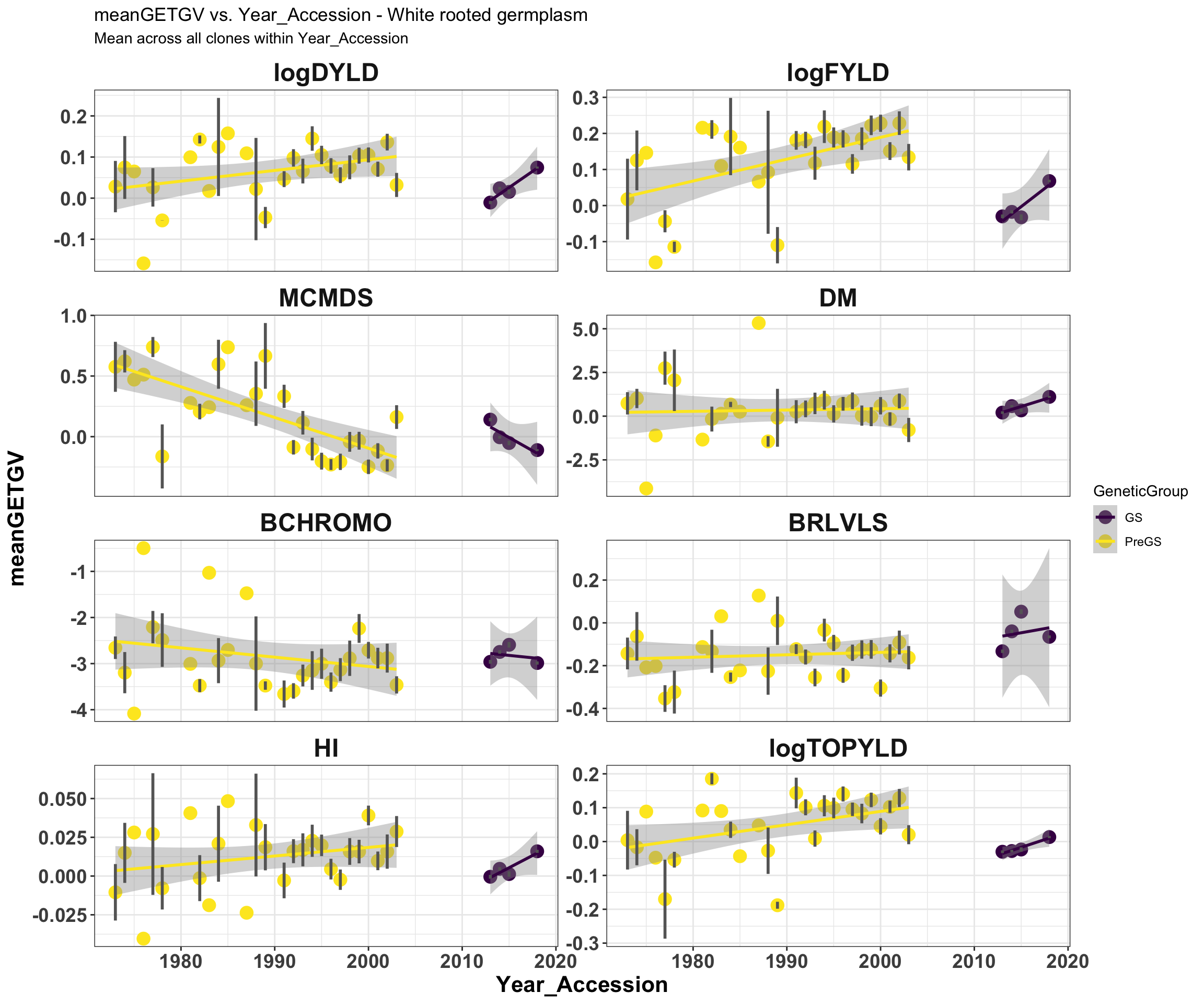
sessionInfo()R version 4.0.2 (2020-06-22)
Platform: x86_64-apple-darwin17.0 (64-bit)
Running under: macOS Catalina 10.15.7
Matrix products: default
BLAS: /Library/Frameworks/R.framework/Versions/4.0/Resources/lib/libRblas.dylib
LAPACK: /Library/Frameworks/R.framework/Versions/4.0/Resources/lib/libRlapack.dylib
locale:
[1] en_US.UTF-8/en_US.UTF-8/en_US.UTF-8/C/en_US.UTF-8/en_US.UTF-8
attached base packages:
[1] stats graphics grDevices utils datasets methods base
other attached packages:
[1] magrittr_2.0.1 forcats_0.5.0 stringr_1.4.0 dplyr_1.0.2
[5] purrr_0.3.4 readr_1.4.0 tidyr_1.1.2 tibble_3.0.4
[9] ggplot2_3.3.2 tidyverse_1.3.0 workflowr_1.6.2
loaded via a namespace (and not attached):
[1] Rcpp_1.0.5 lattice_0.20-41 lubridate_1.7.9.2 here_1.0.0
[5] ps_1.4.0 assertthat_0.2.1 rprojroot_2.0.2 digest_0.6.27
[9] R6_2.5.0 cellranger_1.1.0 backports_1.2.0 reprex_0.3.0
[13] evaluate_0.14 httr_1.4.2 highr_0.8 pillar_1.4.7
[17] rlang_0.4.9 readxl_1.3.1 rstudioapi_0.13 whisker_0.4
[21] Matrix_1.2-18 rmarkdown_2.5 splines_4.0.2 labeling_0.4.2
[25] munsell_0.5.0 broom_0.7.2 compiler_4.0.2 httpuv_1.5.4
[29] modelr_0.1.8 xfun_0.19 pkgconfig_2.0.3 mgcv_1.8-33
[33] htmltools_0.5.0 tidyselect_1.1.0 fansi_0.4.1 viridisLite_0.3.0
[37] crayon_1.3.4 dbplyr_2.0.0 withr_2.3.0 later_1.1.0.1
[41] grid_4.0.2 nlme_3.1-150 jsonlite_1.7.1 gtable_0.3.0
[45] lifecycle_0.2.0 DBI_1.1.0 git2r_0.27.1 formatR_1.7
[49] scales_1.1.1 cli_2.2.0 stringi_1.5.3 farver_2.0.3
[53] fs_1.5.0 promises_1.1.1 xml2_1.3.2 ellipsis_0.3.1
[57] generics_0.1.0 vctrs_0.3.5 tools_4.0.2 glue_1.4.2
[61] hms_0.5.3 yaml_2.2.1 colorspace_2.0-0 rvest_0.3.6
[65] knitr_1.30 haven_2.3.1