Supplementary Figures
2020-July-29
Last updated: 2021-02-01
Checks: 7 0
Knit directory: PredictOutbredCrossVar/
This reproducible R Markdown analysis was created with workflowr (version 1.6.2). The Checks tab describes the reproducibility checks that were applied when the results were created. The Past versions tab lists the development history.
Great! Since the R Markdown file has been committed to the Git repository, you know the exact version of the code that produced these results.
Great job! The global environment was empty. Objects defined in the global environment can affect the analysis in your R Markdown file in unknown ways. For reproduciblity it’s best to always run the code in an empty environment.
The command set.seed(20191123) was run prior to running the code in the R Markdown file. Setting a seed ensures that any results that rely on randomness, e.g. subsampling or permutations, are reproducible.
Great job! Recording the operating system, R version, and package versions is critical for reproducibility.
Nice! There were no cached chunks for this analysis, so you can be confident that you successfully produced the results during this run.
Great job! Using relative paths to the files within your workflowr project makes it easier to run your code on other machines.
Great! You are using Git for version control. Tracking code development and connecting the code version to the results is critical for reproducibility.
The results in this page were generated with repository version 883b1d4. See the Past versions tab to see a history of the changes made to the R Markdown and HTML files.
Note that you need to be careful to ensure that all relevant files for the analysis have been committed to Git prior to generating the results (you can use wflow_publish or wflow_git_commit). workflowr only checks the R Markdown file, but you know if there are other scripts or data files that it depends on. Below is the status of the Git repository when the results were generated:
Ignored files:
    Ignored:    .DS_Store
    Ignored:    .Rhistory
    Ignored:    .Rproj.user/
    Ignored:    analysis/.DS_Store
    Ignored:    code/.DS_Store
    Ignored:    data/.DS_Store
    Ignored:    output/.DS_Store
    Ignored:    output/crossRealizations/.DS_Store

Untracked files:
    Untracked:  .gitignore
    Untracked:  Icon
    Untracked:  PredictOutbredCrossVar.Rproj
    Untracked:  manuscript/
    Untracked:  output/crossPredictions/
    Untracked:  output/gblups_DirectionalDom_parentwise_crossVal_folds.rds
    Untracked:  output/gblups_geneticgroups.rds
    Untracked:  output/gblups_parentwise_crossVal_folds.rds
Note that any generated files, e.g. HTML, png, CSS, etc., are not included in this status report because it is ok for generated content to have uncommitted changes.
These are the previous versions of the repository in which changes were made to the R Markdown (analysis/SupplementaryFigures.Rmd) and HTML (docs/SupplementaryFigures.html) files. If you’ve configured a remote Git repository (see ?wflow_git_remote), click on the hyperlinks in the table below to view the files as they were in that past version.
| File | Version | Author | Date | Message |
|---|---|---|---|---|
| Rmd | 883b1d4 | wolfemd | 2021-02-01 | Update the syntax highlighting and code-block formatting throughout for |
| Rmd | 6a10c30 | wolfemd | 2021-01-04 | Submission and GitHub ready version. |
| html | 6a10c30 | wolfemd | 2021-01-04 | Submission and GitHub ready version. |
library(tidyverse); library(magrittr);Figure S01: Genome-wide proportion homozygous
Figure S01: Boxplot of the genome-wide proportion of homozygous SNPs in each of four genetic groups comprising the study pedigree.
propHom<-readxl::read_xlsx(here::here("manuscript","SupplementaryTables.xlsx"),sheet = "TableS14")
propHom %>%
  mutate(Group=ifelse(!grepl("TMS13|TMS14|TMS15", GID),"GG (C0)",NA),
         Group=ifelse(grepl("TMS13", GID),"TMS13 (C1)",Group),
         Group=ifelse(grepl("TMS14", GID),"TMS14 (C2)",Group),
         Group=ifelse(grepl("TMS15", GID),"TMS15 (C3)",Group)) %>%
  ggplot(.,aes(x=Group,y=PropSNP_homozygous,fill=Group)) + geom_boxplot() +
  theme_bw() +
  scale_fill_viridis_d()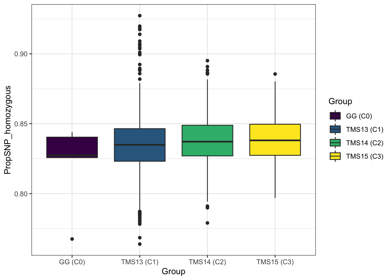
| Version | Author | Date |
|---|---|---|
| 6a10c30 | wolfemd | 2021-01-04 |
Figure S02: Correlations among phenotypic BLUPs (including Selection Indices)
Figure S02: Correlations among BLUPs (including Selection Indices). (A) StdSI vs. BiofortSI computed from i.i.d. BLUPs. (B) Heatmap of the correlation among BLUPs for each of four component traits and two derived selection indices.
library(tidyverse); library(magrittr);
# Selection weights -----------
indices<-readxl::read_xlsx(here::here("manuscript","SupplementaryTables.xlsx"),sheet = "TableS01")
# BLUPs -----------
blups<-readRDS(here::here("data","blups_forawcdata.rds")) %>%
  select(Trait,blups) %>%
  unnest(blups) %>%
  select(Trait,germplasmName,BLUP) %>%
  spread(Trait,BLUP) %>%
  select(germplasmName,all_of(c("DM","logFYLD","MCMDS","TCHART")))
blups %<>%
  select(germplasmName,all_of(indices$Trait)) %>%
  mutate(stdSI=blups %>%
           select(all_of(indices$Trait)) %>%
           as.data.frame(.) %>%
           as.matrix(.)%*%indices$stdSI,
         biofortSI=blups %>%
           select(all_of(indices$Trait)) %>%
           as.data.frame(.) %>%
           as.matrix(.)%*%indices$biofortSI)
#```{r, fig.show="hold", out.width="50%"}
library(patchwork)
p1<-ggplot(blups,aes(x=stdSI,y=biofortSI)) + geom_point(size=1.25) + theme_bw()
corMat<-cor(blups[,-1],use = 'pairwise.complete.obs')
(p1 | ~corrplot::corrplot(corMat, type = 'lower', col = viridis::viridis(n = 10), diag = T,addCoef.col = "black")) +
plot_layout(nrow=1, widths = c(0.35,0.65)) +
plot_annotation(tag_levels = 'A',
title = 'Correlations among phenotypic BLUPs (including Selection Indices)')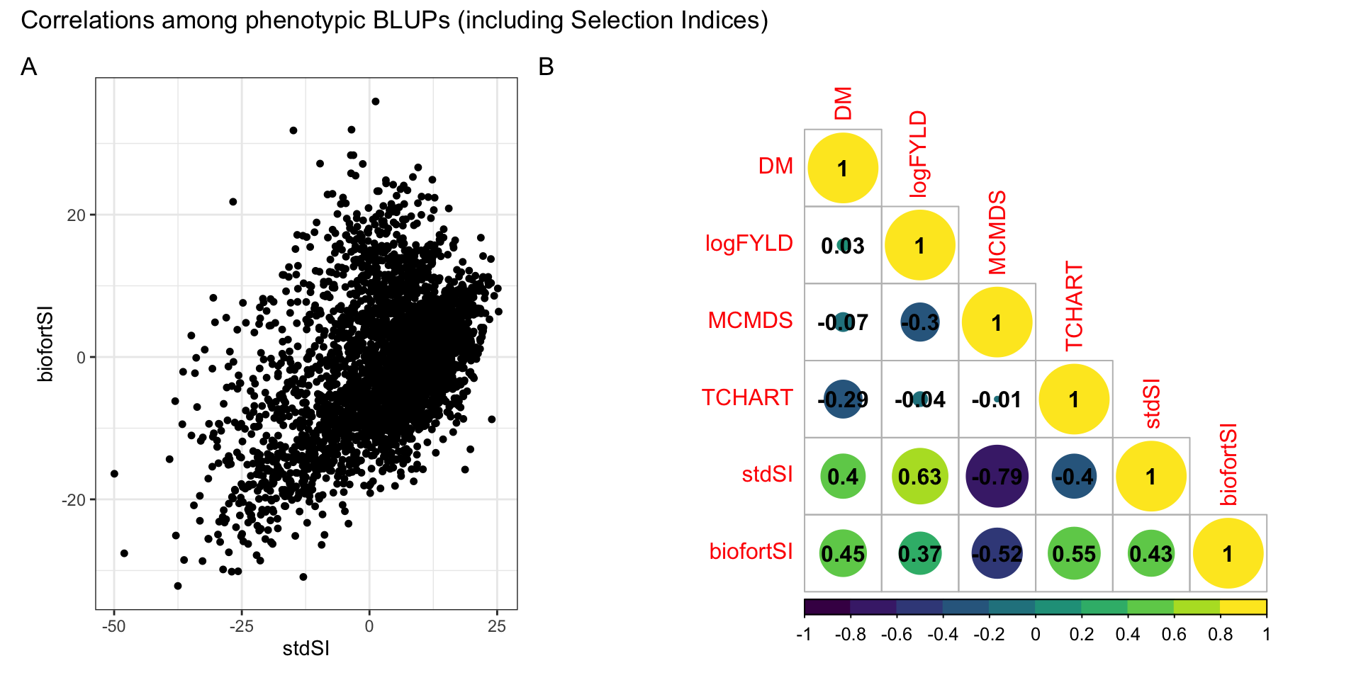
| Version | Author | Date |
|---|---|---|
| 6a10c30 | wolfemd | 2021-01-04 |
Figure S03: Scatterplot comparing accuracies for family means using different validation-data
Figure S03: Scatterplot comparing accuracies for family means using different validation-data.
library(tidyverse); library(magrittr);
# Table S10: Accuracies predicting the mean
accMeans<-readxl::read_xlsx(here::here("manuscript","SupplementaryTables.xlsx"),sheet = "TableS10")
accMeans %>% #count(ValidationData,Model,VarComp)
  spread(ValidationData,Accuracy) %>%
  ggplot(.,aes(x=iidBLUPs,y=GBLUPs,color=predOf,shape=Trait)) +
  geom_point() +
  geom_abline(slope=1,color='darkred') +
  facet_wrap(~predOf+Model,scales = 'free') +
  theme_bw() + scale_color_viridis_d() +
  labs(title = "Scatterplot comparing accuracies for family means using different validation-data")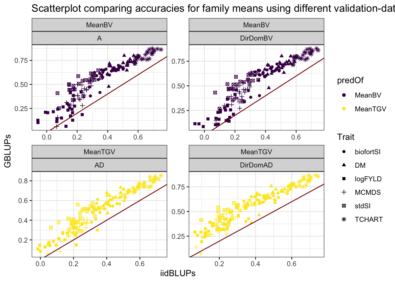
| Version | Author | Date |
|---|---|---|
| 6a10c30 | wolfemd | 2021-01-04 |
Figure S04: Accuracies per trait-fold-rep-Model do not re-rank much from iid-to-GBLUP validation data
Figure S04: Boxplots to show that Accuracies per trait-fold-rep-Model do not re-rank much whether using the iid or the GBLUPs as validation data.
forplot<-accMeans %>%
  mutate(Pred=paste0(predOf,"_",Model),
         Pred=factor(Pred,levels=c("MeanBV_A","MeanBV_DirDomBV","MeanTGV_AD","MeanTGV_DirDomAD")),
         Trait=factor(Trait,levels=c("stdSI","biofortSI","DM","logFYLD","MCMDS","TCHART")),
         predOf=factor(predOf,levels=c("MeanBV","MeanTGV")),
         Model=factor(Model,levels=c("A","AD","DirDomBV","DirDomAD")),
         RepFold=paste0(Repeat,"_",Fold,"_",Trait))

forplot %>%
  ggplot(aes(x=ValidationData,y=Accuracy)) +
  geom_violin(data=forplot,aes(fill=ValidationData), alpha=0.75) +
  geom_boxplot(data=forplot,aes(fill=ValidationData), alpha=0.85, color='gray',width=0.2) +
  geom_line(data=forplot,aes(group=RepFold),color='darkred',size=0.6,alpha=0.8) +
  geom_point(data=forplot,aes(color=ValidationData, group=RepFold),size=1.5) +
  theme_bw() +
  scale_fill_viridis_d(option = "A") +
  scale_color_viridis_d() +
  theme(axis.text.x = element_text(face='bold', size=10, angle=90),
        axis.text.y = element_text(face='bold', size=10)) +
  facet_grid(Trait~Pred, scales='free_y') +
  labs(title = "Accuracies per trait-fold-rep-Model do not re-rank much from iid-to-GBLUP validation data")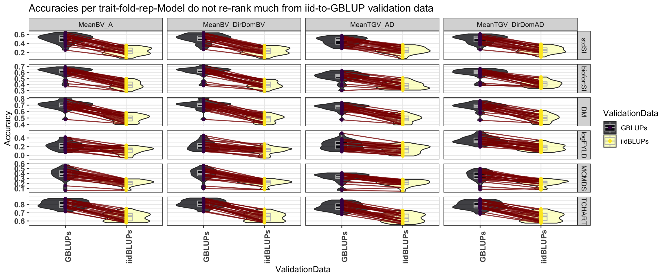
| Version | Author | Date |
|---|---|---|
| 6a10c30 | wolfemd | 2021-01-04 |
Figure S05: Accuracy predicting family means - GBLUP vs. iid-BLUPs as validation data
Figure S05: Accuracy predicting family means - GBLUP vs. iid-BLUPs as validation data. Fivefold parent-wise cross-validation estimates of the accuracy predicting the cross means on selection indices and for component traits (x-axis), summarized in boxplots. Accuracy (y-axis) was measured as the correlation between the predicted and the observed mean GEBV or GETGV. For each trait, accuracies for four predictions: two prediction types (family mean BV vs. TGV) times two prediction models (Classic vs. DirDom). Validation data (GBLUPs vs. iidBLUPs) are shown in two horizontal panels.
accMeans %>%
  mutate(Pred=paste0(predOf,"_",Model),
         Pred=factor(Pred,levels=c("MeanBV_A","MeanBV_DirDomBV","MeanTGV_AD","MeanTGV_DirDomAD")),
         Trait=factor(Trait,levels=c("stdSI","biofortSI","DM","logFYLD","MCMDS","TCHART")),
         predOf=factor(predOf,levels=c("MeanBV","MeanTGV")),
         Model=factor(Model,levels=c("A","AD","DirDomBV","DirDomAD"))) %>%
  ggplot(.,aes(x=Trait,y=Accuracy,fill=Pred,linetype=predOf)) +
  geom_boxplot() + theme_bw() + scale_fill_viridis_d() +
  geom_hline(yintercept = 0, color='darkred', size=1.5) +
  theme(axis.text.x = element_text(face='bold', size=10, angle=90),
        axis.text.y = element_text(face='bold', size=10)) +
    facet_grid(.~ValidationData) +
  labs(title = "Accuracy predicting family means",
       subtitle = "GBLUP vs. iid-BLUPs as validation data")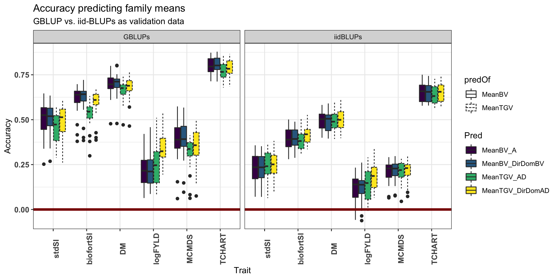
| Version | Author | Date |
|---|---|---|
| 6a10c30 | wolfemd | 2021-01-04 |
Figure S06: The difference between PMV and VPM for variance and covariance predictions
Figure S06: The difference between PMV and VPM for variance and covariance predictions. Each boxplot shows the posterior mean variance (PMV) minus the variance of posterior means (VPM) based prediction of cross variances and covariances. Each panel is a variance or covariance. Each boxplot shows either an additive or dominance variance from one of the genetic models (x-axis).
## Table S7: Predicted cross variances
predVars<-read.csv(here::here("manuscript","SupplementaryTable07.csv"),stringsAsFactors = F)
predVars %>%
  mutate(VarCovar=paste0(Trait1,"_",Trait2),
         Pred=paste0(Model,"_",VarComp),
         diffPredVar=PMV-VPM) %>%
  ggplot(.,aes(x=Pred,y=diffPredVar,fill=Pred,linetype=VarComp)) +
  geom_boxplot() + facet_wrap(~VarCovar,scales='free',nrow=2) +
  geom_hline(yintercept = 0) + theme_bw() +
  theme(axis.text.x = element_text(angle=90)) +
  scale_fill_viridis_d() +
  labs(title="The difference between PMV and VPM for variance and covariance predictions",
       y="diffPredVar = PMV minus VPM ")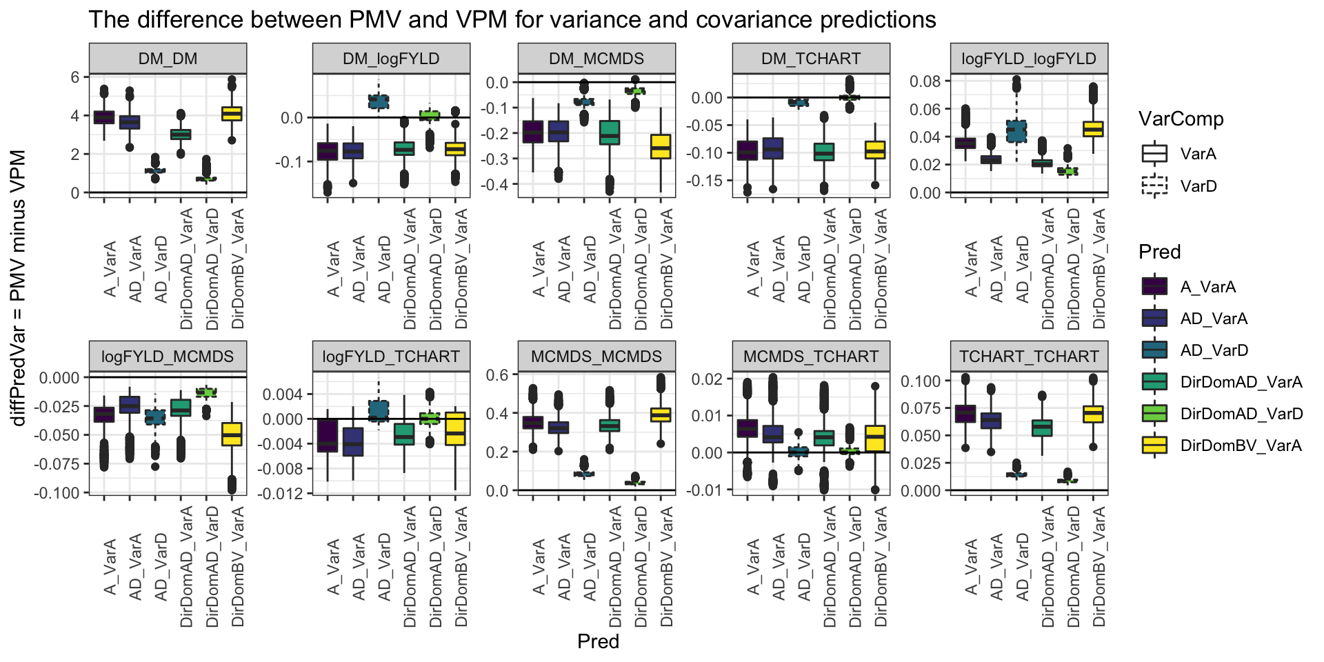
| Version | Author | Date |
|---|---|---|
| 6a10c30 | wolfemd | 2021-01-04 |
Figure S07: The difference between PMV and VPM in terms of prediction accuracy
Figure S07: The difference between PMV and VPM in terms of prediction accuracy. Each boxplot shows the posterior mean variance (PMV) minus the variance of posterior means (VPM) based estimate of prediction accuracy for cross variances and covariances. Each panel is a variance or covariance. Each boxplot shows either an additive or dominance variance from one of the genetic models (x-axis).
## Table S11: Accuracies predicting the variances
accVars<-readxl::read_xlsx(here::here("manuscript","SupplementaryTables.xlsx"),sheet = "TableS11")
accVars %>%
  select(-AccuracyCor) %>%
  spread(VarMethod,AccuracyWtCor) %>%
  mutate(VarCovar=paste0(Trait1,"_",Trait2),
         Pred=paste0(Model,"_",predOf),
         diffAcc=PMV-VPM) %>%
  ggplot(.,aes(x=Pred,y=diffAcc,fill=Pred,linetype=predOf)) +
  geom_boxplot() + facet_wrap(~VarCovar,scales='free',nrow=2) +
  geom_hline(yintercept = 0) + theme_bw() +
  theme(axis.text.x = element_text(angle=90)) +
  scale_fill_viridis_d() +
  labs(title="The difference between PMV and VPM in terms of prediction accuracy",
       y="diffPredAcc = predAccPMV minus predAccVPM",x=NULL)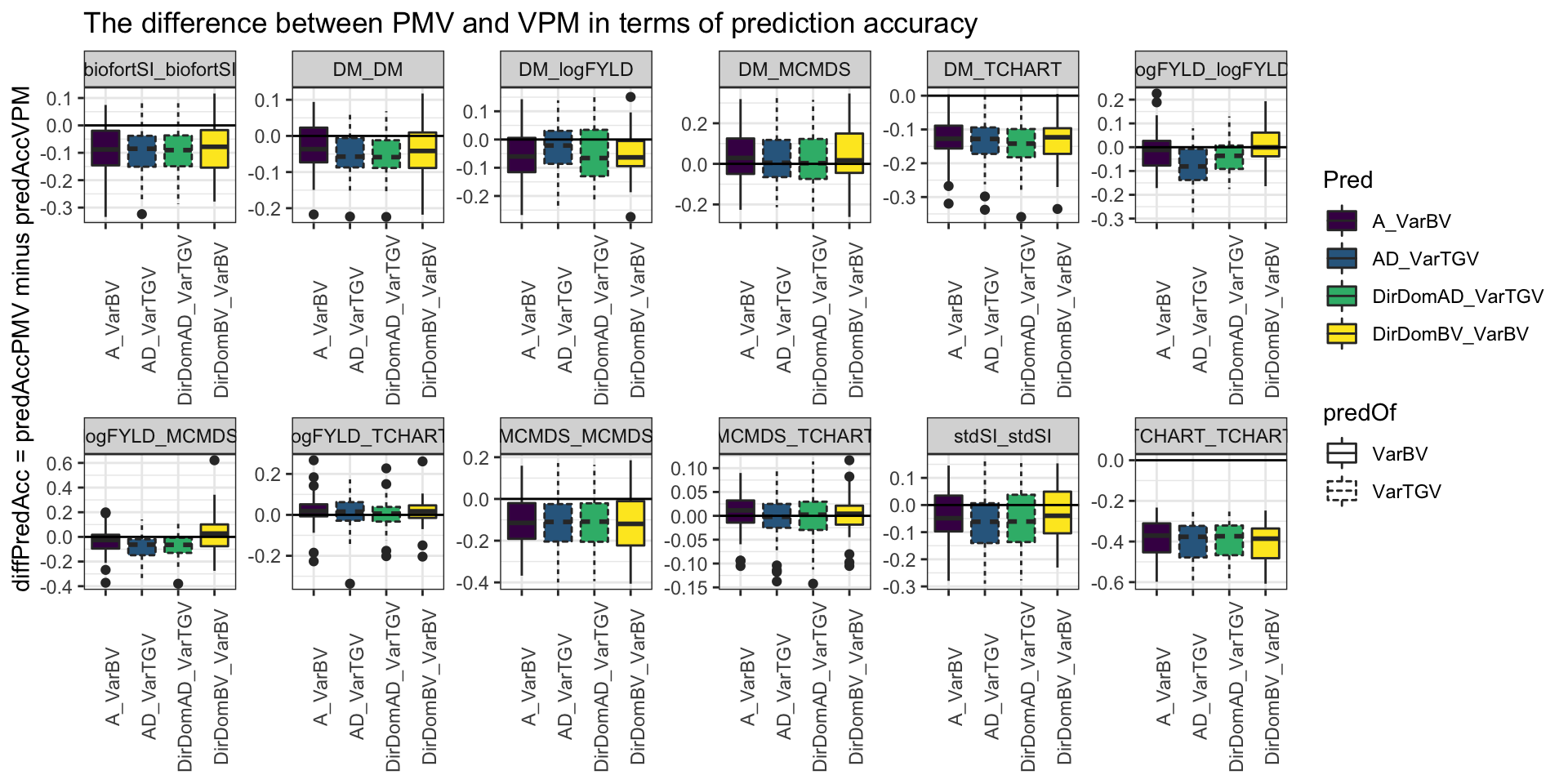
| Version | Author | Date |
|---|---|---|
| 6a10c30 | wolfemd | 2021-01-04 |
Figure S08: Scatterplot comparing accuracies for family (co)variances using different validation-data
Figure S08: Scatterplot comparing accuracies for family variance and covariance prediction using different validation-data.
## Table S11: Accuracies predicting the variances
accVars<-readxl::read_xlsx(here::here("manuscript","SupplementaryTables.xlsx"),sheet = "TableS11")

accVars %>%
  filter(VarMethod=="PMV") %>%
  select(-AccuracyCor) %>%
  spread(ValidationData,AccuracyWtCor) %>%
  mutate(Component=paste0(Trait1,"_",Trait2)) %>%
  ggplot(.,aes(x=iidBLUPs,y=GBLUPs,shape=predOf,color=Component)) +
  geom_point() +
  geom_abline(slope=1,color='darkred') +
  facet_wrap(~predOf+Model,scales = 'free') +
  theme_bw() + scale_color_viridis_d(option = "B") +
  labs(title = "Scatterplot comparing accuracies for different validation-data",
       subtitle = "Family (co)variances")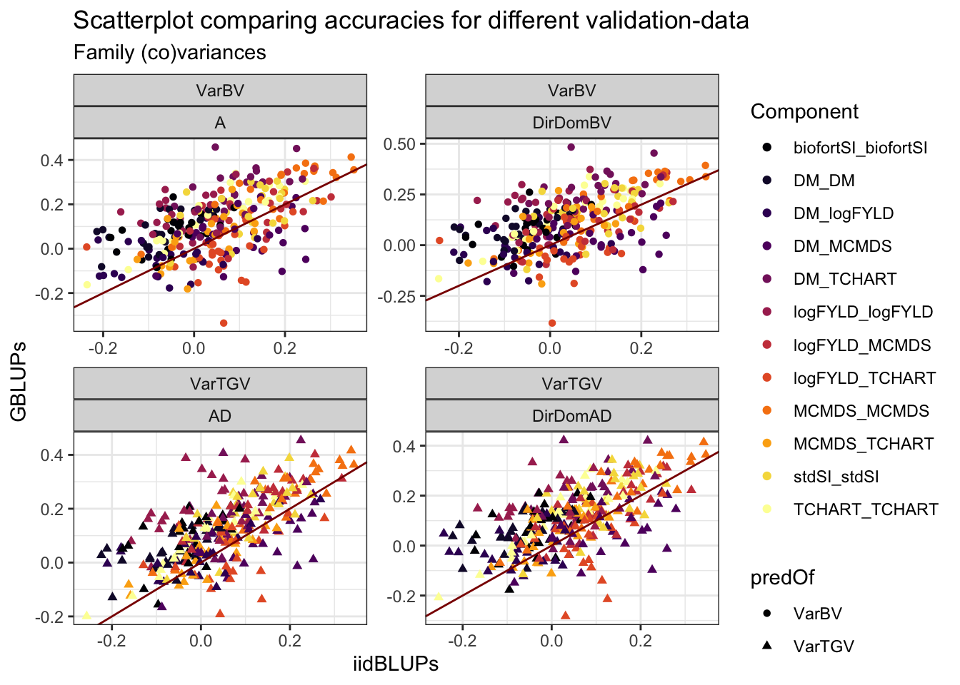
| Version | Author | Date |
|---|---|---|
| 6a10c30 | wolfemd | 2021-01-04 |
Figure S09: Plot of variance-prediction accuracy: Re-ranking according choice of validation?
Figure S09: Plot of variance-prediction accuracy to show whether re-ranking occurrs according to the choice of validation data (x-axis), GBLUPs vs. i.i.d. BLUPs.
forplot<-accVars %>%
  filter(VarMethod=="PMV") %>%
  filter(Trait1==Trait2,grepl("SI",Trait1)) %>%
  mutate(Pred=paste0(predOf,"_",Model),
         Pred=factor(Pred,levels=c("VarBV_A","VarBV_DirDomBV","VarTGV_AD","VarTGV_DirDomAD")),
         Trait1=factor(Trait1,levels=c("stdSI","biofortSI")),#,"DM","logFYLD","MCMDS","TCHART")),
         Trait2=factor(Trait2,levels=c("stdSI","biofortSI")),#,"DM","logFYLD","MCMDS","TCHART")),
         Component=paste0(Trait1,"_",Trait2),
         predOf=factor(predOf,levels=c("VarBV","VarTGV")),
         Model=factor(Model,levels=c("A","AD","DirDomBV","DirDomAD")),
         RepFold=paste0(Repeat,"_",Fold,"_",Component))

forplot %>%
  ggplot(aes(x=ValidationData,y=AccuracyWtCor)) +
  geom_violin(data=forplot,aes(fill=ValidationData), alpha=0.75) +
  geom_boxplot(data=forplot,aes(fill=ValidationData), alpha=0.85, color='gray',width=0.2) +
  geom_line(data=forplot,aes(group=RepFold),color='darkred',size=0.6,alpha=0.8) +
  geom_point(data=forplot,aes(color=ValidationData, group=RepFold),size=1.5) +
  theme_bw() +
  scale_fill_viridis_d(option = "A") +
  scale_color_viridis_d() +
  theme(axis.text.x = element_text(face='bold', size=10, angle=90),
        axis.text.y = element_text(face='bold', size=10)) +
  facet_grid(Component~Pred, scales='free_y') +
  labs(title="Plot of variance-prediction accuracy: Re-ranking according choice of validation?")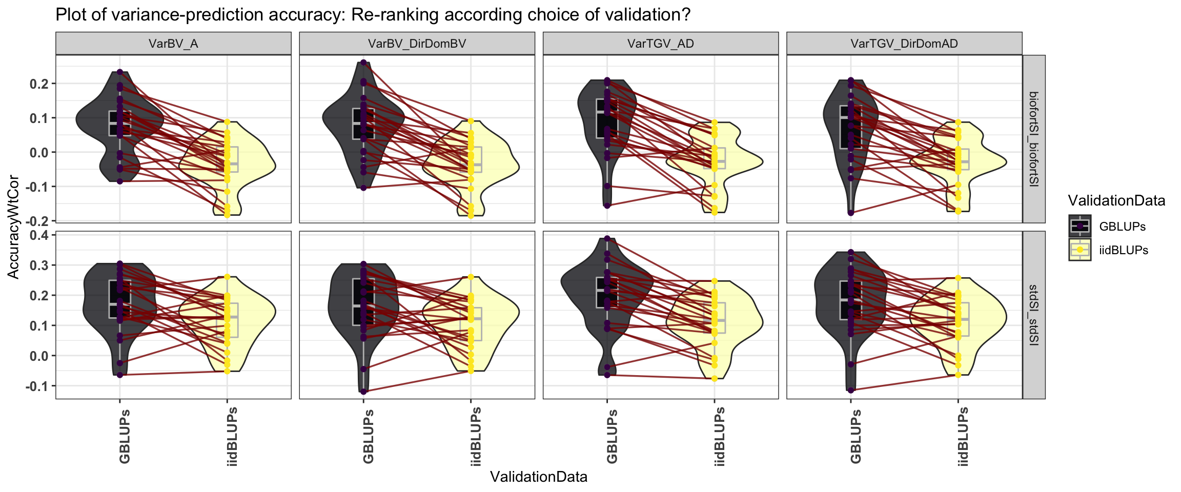
| Version | Author | Date |
|---|---|---|
| 6a10c30 | wolfemd | 2021-01-04 |
Figure S10: Accuracy predicting family variances - GBLUP vs. iid-BLUPs as validation data
Figure S10: Accuracy predicting family variances - GBLUP vs. iid-BLUPs as validation data. Fivefold parent-wise cross-validation estimates of the accuracy predicting (A) genetic variances and (B) covariances. Selection indices and component trait variances are shown on the x-axis. Accuracy (y-axis) was measured as the weighted correlation between the predicted and the observed (co)variance of GEBV or GETGV. For each trait (panel), accuracies for four predictions: two prediction types (VarBV vs. VarTGV) times two prediction models (Classic vs. DirDom). Validation data (GBLUPs vs. iidBLUPs) are shown in horizontal panels.
forplot<-accVars %>%
  filter(VarMethod=="PMV") %>%
  mutate(Pred=paste0(predOf,"_",Model),
         Pred=factor(Pred,levels=c("VarBV_A","VarTGV_AD","VarBV_DirDomBV","VarTGV_DirDomAD")),
         Trait1=factor(Trait1,levels=c("stdSI","biofortSI","DM","logFYLD","MCMDS","TCHART")),
         Trait2=factor(Trait2,levels=c("stdSI","biofortSI","DM","logFYLD","MCMDS","TCHART")),
         Component=paste0(Trait1,"_",Trait2),
         predOf=factor(predOf,levels=c("VarBV","VarTGV")),
         Model=factor(Model,levels=c("A","AD","DirDomBV","DirDomAD")),
         RepFold=paste0(Repeat,"_",Fold,"_",Component))

p_vars<-forplot %>%
  filter(Trait1==Trait2) %>%
  ggplot(.,aes(x=Component,y=AccuracyWtCor,fill=Pred,linetype=predOf)) +
  geom_boxplot() + theme_bw() + scale_fill_viridis_d() +
  geom_hline(yintercept = 0, color='darkred', size=1.5) +
  theme(axis.text.x = element_text(face='bold', size=8, angle=90),
        axis.text.y = element_text(face='bold', size=10)) +
  facet_wrap(~ValidationData,scales='free') +
  ggtitle(expression(paste("Plot of ", underline(variance), "-prediction accuracy")))
p_covars<-forplot %>%
  filter(VarMethod=="PMV") %>%
  filter(Trait1!=Trait2) %>%
  ggplot(.,aes(x=Component,y=AccuracyWtCor,fill=Pred,linetype=predOf)) +
  geom_boxplot() + theme_bw() + scale_fill_viridis_d() +
  geom_hline(yintercept = 0, color='darkred', size=1.5) +
  theme(axis.text.x = element_text(face='bold', size=8, angle=90),
        axis.text.y = element_text(face='bold', size=10)) +
  facet_wrap(~ValidationData,scales='free') +
  ggtitle(expression(paste("Plot of ", underline(co), "variance-prediction accuracy")))
#  labs(subtitle="GBLUPs vs. iidBLUPs as validation-data")
require(patchwork)
(p_vars / p_covars) +
plot_layout(nrow=2,guides = 'collect') +
plot_annotation(tag_levels = 'A',
title = 'Accuracy predicting family (co)variances - GBLUP vs. iid-BLUPs as validation data')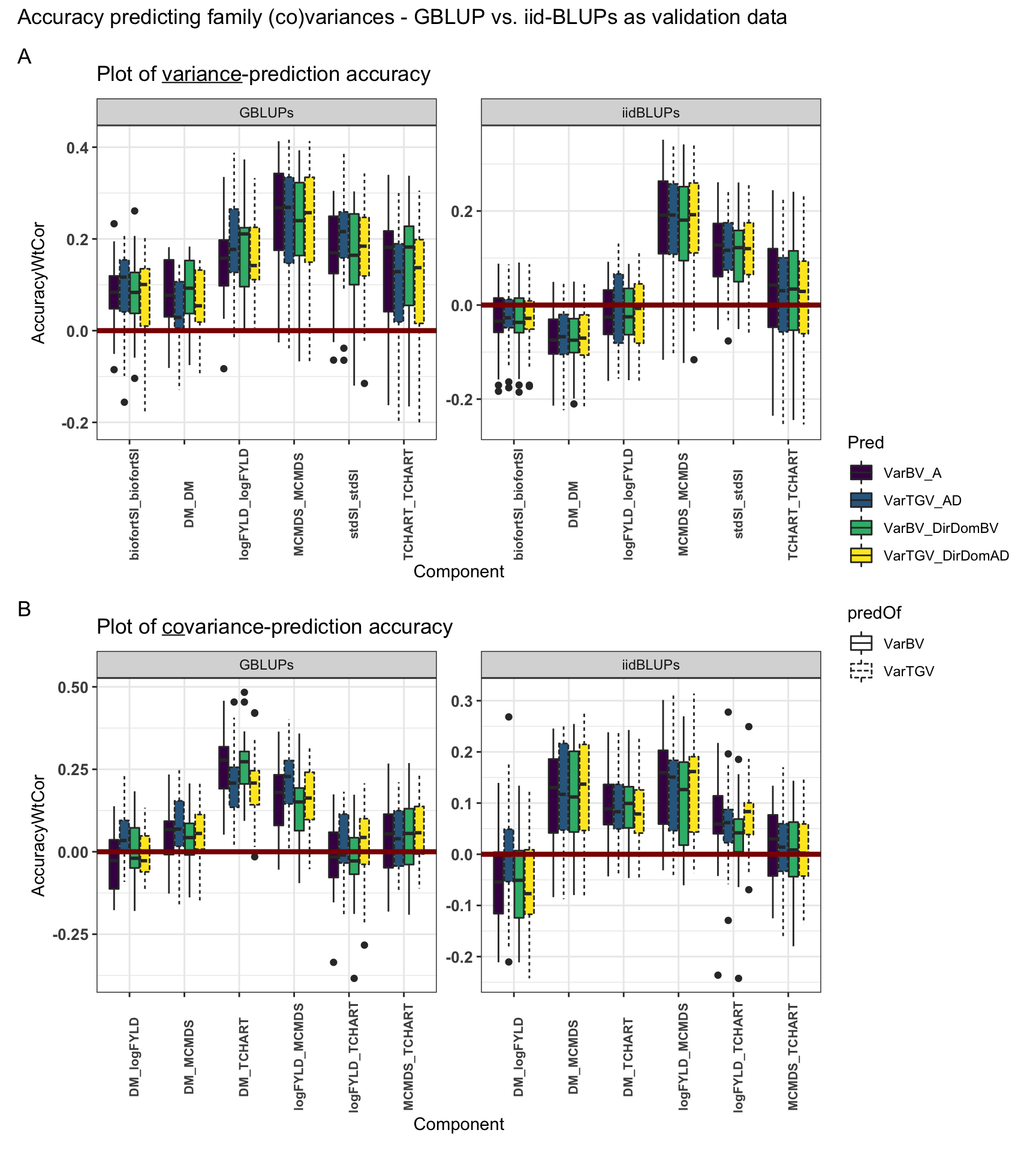
| Version | Author | Date |
|---|---|---|
| 6a10c30 | wolfemd | 2021-01-04 |
Figure S11: Accuracy predicting family (co)variances - Weighted vs. Unweighted Correlation
Figure S11: Accuracy predicting family (co)variances - Weighted vs. Unweighted Correlation. Fivefold parent-wise cross-validation estimates of the accuracy predicting (A) genetic variances and (B) covariances. Selection indices and component trait variances are shown on the x-axis. Accuracy (y-axis) was measured as the (weighted or unweighted) correlation between the predicted and the observed (co)variance of GEBV or GETGV. For each trait (panel), accuracies for four predictions: two prediction types (VarBV vs. VarTGV) times two prediction models (Classic vs. DirDom). Weighted vs. Unweighted Correlations as accuracy estimates are shown in horizontal panels.
forplot<-accVars %>%
  filter(VarMethod=="PMV",ValidationData=="GBLUPs") %>%
  pivot_longer(cols=contains("Cor"),names_to = "WT_or_NoWT", values_to = "Accuracy") %>%
   mutate(Pred=paste0(predOf,"_",Model),
         Pred=factor(Pred,levels=c("VarBV_A","VarTGV_AD","VarBV_DirDomBV","VarTGV_DirDomAD")),
         Trait1=factor(Trait1,levels=c("stdSI","biofortSI","DM","logFYLD","MCMDS","TCHART")),
         Trait2=factor(Trait2,levels=c("stdSI","biofortSI","DM","logFYLD","MCMDS","TCHART")),
         Component=paste0(Trait1,"_",Trait2),
         predOf=factor(predOf,levels=c("VarBV","VarTGV")),
         Model=factor(Model,levels=c("A","AD","DirDomBV","DirDomAD")),
         RepFold=paste0(Repeat,"_",Fold,"_",Component))


p_vars<-forplot %>%
  filter(Trait1==Trait2) %>%
  ggplot(.,aes(x=Component,y=Accuracy,fill=Pred,linetype=predOf)) +
  geom_boxplot() + theme_bw() + scale_fill_viridis_d() +
  geom_hline(yintercept = 0, color='darkred', size=1.5) +
  theme(axis.text.x = element_text(face='bold', size=9, angle=90),
        axis.text.y = element_text(face='bold', size=10)) +
  facet_wrap(~WT_or_NoWT,scales='free') +
  ggtitle(expression(paste("Plot of ", underline(variance), "-prediction accuracy")))
p_covars<-forplot %>%
  filter(Trait1!=Trait2) %>%
  ggplot(.,aes(x=Component,y=Accuracy,fill=Pred,linetype=predOf)) +
  geom_boxplot() + theme_bw() + scale_fill_viridis_d() +
  geom_hline(yintercept = 0, color='darkred', size=1.5) +
  theme(axis.text.x = element_text(face='bold', size=9, angle=90),
        axis.text.y = element_text(face='bold', size=10)) +
  facet_wrap(~WT_or_NoWT,scales='free') +
  ggtitle(expression(paste("Plot of ", underline(co), "variance-prediction accuracy")))
(p_vars / p_covars) +
plot_layout(nrow=2,guides = 'collect') +
plot_annotation(tag_levels = 'A',
title = 'Accuracy predicting family (co)variances - Weighted vs. Unweighted Correlation',
subtitle = "GBLUPs as validation-data")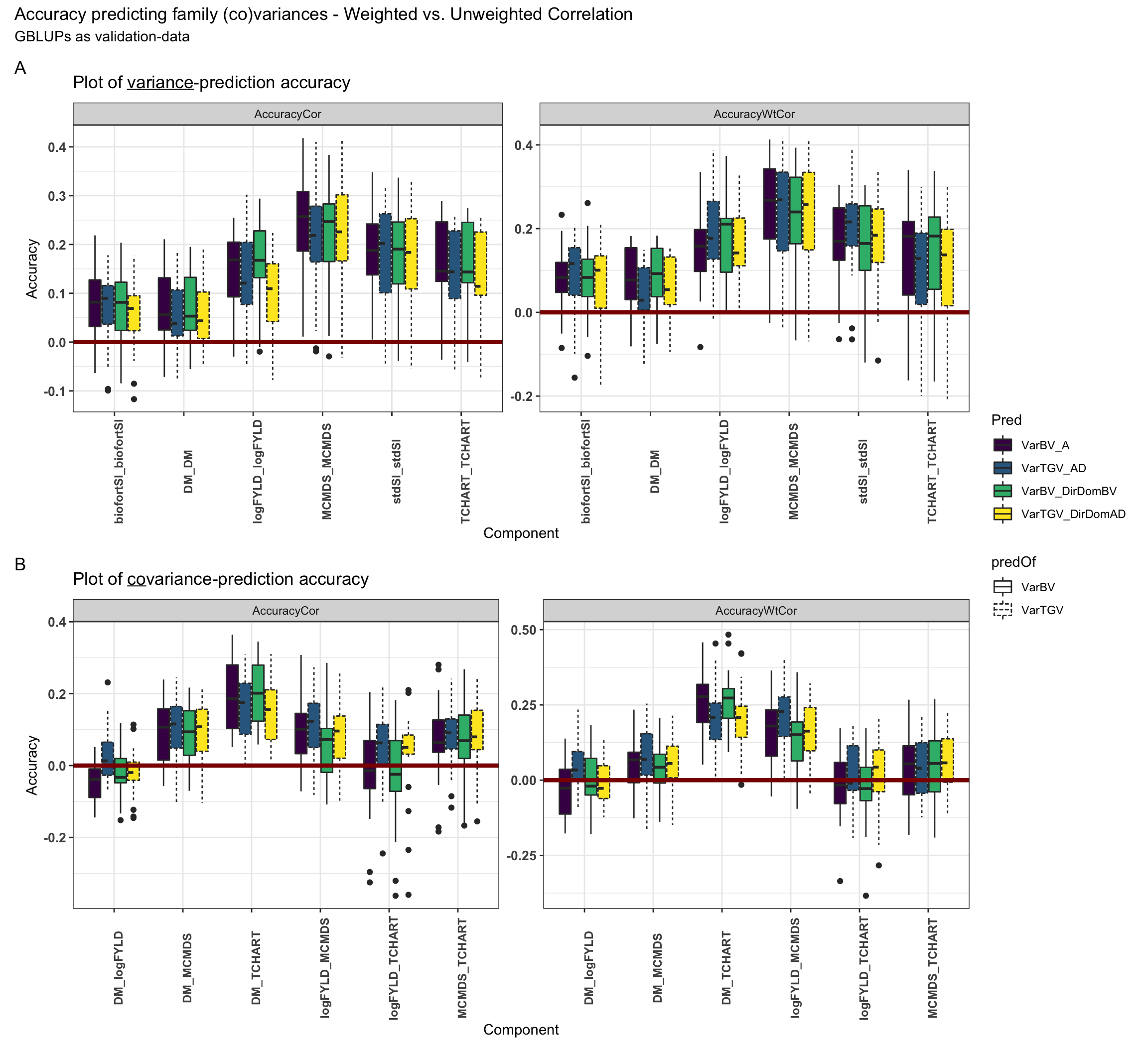
| Version | Author | Date |
|---|---|---|
| 6a10c30 | wolfemd | 2021-01-04 |
Figure S12: Realized selection intensities: measuring post-cross selection
Figure S12: Realized selection intensities: measuring post-cross selection. Boxplots showing (A) the proportion of each family selected and (B) the standardized selection intensity for each stage of the breeding pipeline, in each genetic group.
library(patchwork)
## Table S13: Realized within-cross selection metrics
crossmetrics<-readxl::read_xlsx(here::here("manuscript","SupplementaryTables.xlsx"),sheet = "TableS13")
propPast<-crossmetrics %>%
  mutate(Cycle=ifelse(!grepl("TMS13|TMS14|TMS15",sireID) & !grepl("TMS13|TMS14|TMS15",damID),"C0",
                      ifelse(grepl("TMS13",sireID) | grepl("TMS13",damID),"C1",
                             ifelse(grepl("TMS14",sireID) | grepl("TMS14",damID),"C2",
                                    ifelse(grepl("TMS15",sireID) | grepl("TMS15",damID),"C3","mixed"))))) %>%
  select(Cycle,starts_with("prop")) %>%
  pivot_longer(cols = contains("prop"),values_to = "PropPast",names_to = "StagePast",names_prefix = "propPast|prop") %>%
  rename(DescendentsOfCycle=Cycle) %>%
  mutate(StagePast=gsub("UsedAs","",StagePast),
         StagePast=factor(StagePast,levels=c("Parent","Phenotyped","CET","PYT","AYT"))) %>%
  ggplot(.,aes(x=StagePast,y=PropPast,fill=DescendentsOfCycle)) +
  geom_boxplot(position = 'dodge2',color='black') +
  theme_bw() + scale_fill_viridis_d()  + labs(y="Proportion of Family Selected") +
  theme(legend.position = 'none')
realIntensity<-crossmetrics %>%
  mutate(Cycle=ifelse(!grepl("TMS13|TMS14|TMS15",sireID) & !grepl("TMS13|TMS14|TMS15",damID),"C0",
                      ifelse(grepl("TMS13",sireID) | grepl("TMS13",damID),"C1",
                             ifelse(grepl("TMS14",sireID) | grepl("TMS14",damID),"C2",
                                    ifelse(grepl("TMS15",sireID) | grepl("TMS15",damID),"C3","mixed"))))) %>%
  select(Cycle,sireID,damID,contains("realIntensity")) %>%
  pivot_longer(cols = contains("realIntensity"),names_to = "Stage", values_to = "Intensity",names_prefix = "realIntensity") %>%
  rename(DescendentsOfCycle=Cycle) %>%
  distinct %>% ungroup() %>%
  mutate(Stage=factor(Stage,levels=c("Parent","CET","PYT","AYT","UYT"))) %>%
  ggplot(.,aes(x=Stage,y=Intensity,fill=DescendentsOfCycle)) +
  geom_boxplot(position = 'dodge2',color='black') +
  theme_bw() + scale_fill_viridis_d()  + labs(y="Stadardized Selection Intensity")
propPast + realIntensity +
  plot_annotation(tag_levels = 'A',
                  title = 'Realized selection intensities: measuring post-cross selection') &
  theme(plot.title = element_text(size = 14, face='bold'),
        plot.tag = element_text(size = 13, face='bold'),
        strip.text.x = element_text(size=11, face='bold'))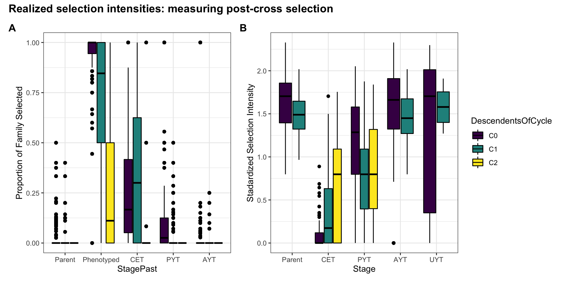
| Version | Author | Date |
|---|---|---|
| 6a10c30 | wolfemd | 2021-01-04 |
Figure S13: Accuracy Predicting Usefulness Criteria - All comparisons
Figure S13: Accuracy Predicting Usefulness Criteria - All comparisons. Accuracy predicting the usefulness (the expected mean of future selected offspring) of previously untested crosses. Fivefold parent-wise cross-validation estimates of the accuracy predicting the usefulness of crosses on the selection indices (x-axes) is summarized in boxplots. Accuracy (y-axis) was measured as the correlation between the predicted and observed usefulness of crosses for each breeding pipeline stage as well as at a constant selection intensity (x-axis). For each UC (panels), accuracies for four predictions: two selection indices (StdSI and BiofortSI) times two prediction models (Classic vs. DirDom).
library(tidyverse); library(magrittr);
## Table S12: Accuracies predicting the usefulness criteria
accUC<-readxl::read_xlsx(here::here("manuscript","SupplementaryTables.xlsx"),sheet = "TableS12")
accUC %>%
  filter(VarMethod=="PMV") %>%
  mutate(Trait=factor(Trait,levels=c("stdSI","biofortSI")),
         Model=ifelse(Model %in% c("A","AD"),"Classic","DirDom"),#gsub("ClassicAD","Classic",Model),
         Pred=paste0(predOf,"_",Model),
         Pred=factor(Pred,levels=c("BV_Classic","TGV_Classic","BV_DirDom","TGV_DirDom")),
         Model=factor(Model,levels=c("Classic","DirDom")),
         predOf=factor(predOf,levels=c("BV","TGV")),
         Stage=factor(Stage,levels = c("ConstIntensity","Parent","CET","PYT","AYT","UYT"))) %>%
  ggplot(.,aes(x=Stage,y=AccuracyWtCor,fill=Pred)) +
  geom_boxplot(position = position_dodge2(padding=0.35), size=1,color='black') +
  theme_bw() +
  scale_fill_viridis_d() +
  scale_color_viridis_d() +
  geom_hline(yintercept = 0, color='darkred', size=1) +
  facet_grid(.~Trait, scales='free_y') +
  labs(y = "Accuracy",
       title = "Accuracy Predicting Usefulness Criteria - All Stages") +
  theme(axis.text = element_text(colour = 'black'),
        axis.text.x = element_text(face='bold',size=20,angle=45, hjust=1),
        axis.title.x = element_blank(),#text(face='bold',size=13),
        axis.text.y = element_text(face='bold', size=20),
        axis.title.y = element_text(face='bold', size=22),
        strip.background.x = element_blank(),
        strip.text.x = element_text(face='bold', size=26),
        plot.title = element_text(size = 14, face='bold'),
        legend.title = element_blank(),
        legend.text = element_text(face='bold',size=22)) +
  labs(y = "Accuracy")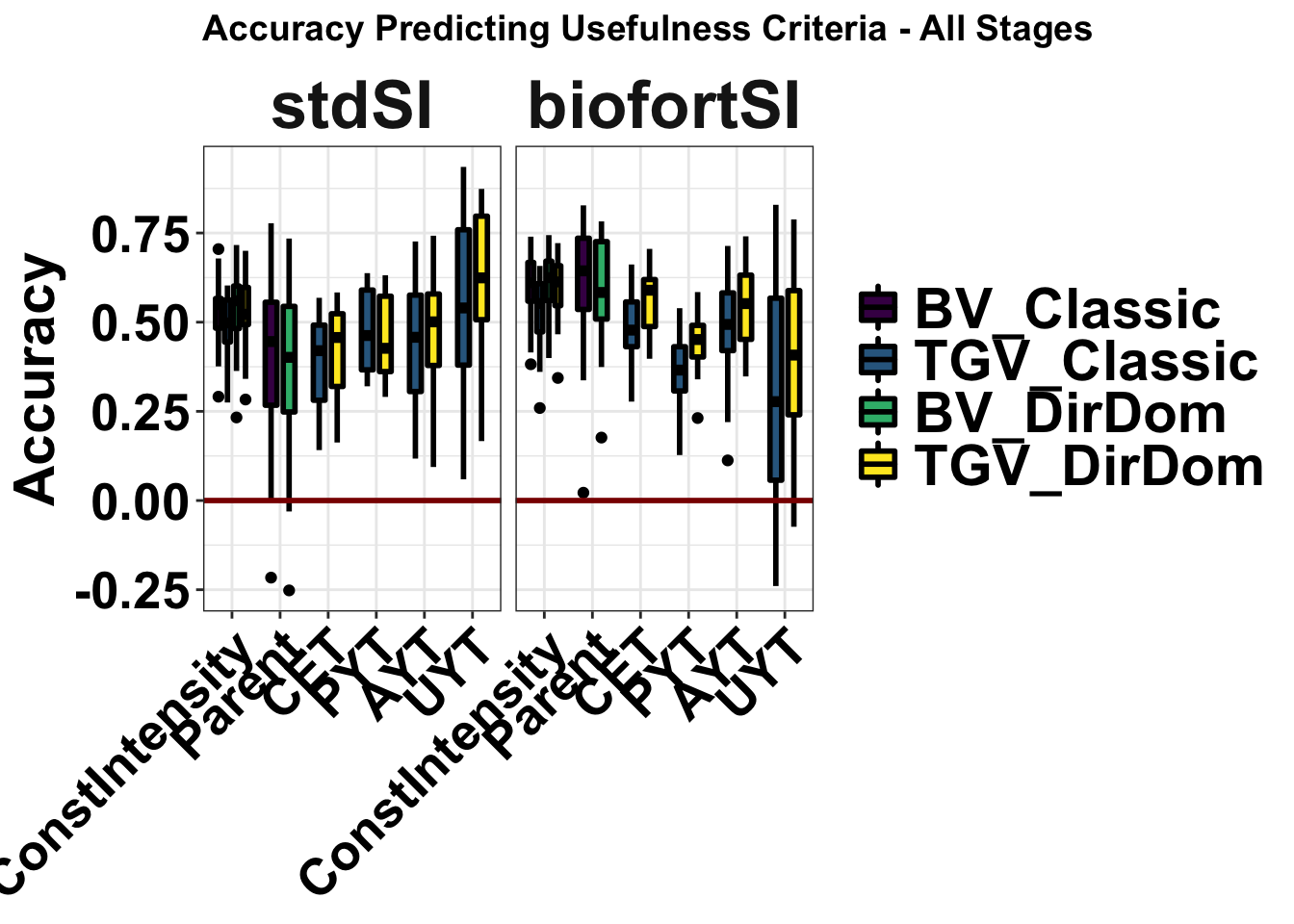
| Version | Author | Date |
|---|---|---|
| 6a10c30 | wolfemd | 2021-01-04 |
Figure S14: Correlation matrix for predictions on the StdSI
Figure S14: Correlation matrix for predictions on the StdSI. Heatmap of the correlations between predictions of mean, standard deviation, and usefulness in terms of BV and TGV, for both the classic and directional dominance model. Predictions were made for 47,083 possible pairwise crosses of 306 parents.
library(tidyverse); library(magrittr);
predUntestedCrosses<-read.csv(here::here("manuscript","SupplementaryTable18.csv"),stringsAsFactors = F)
forCorrMat<-predUntestedCrosses %>%
  mutate(Family=paste0(sireID,"x",damID),
         PredOf=paste0(Trait,"_",PredOf,"_",Component,"_",ifelse(Model=="ClassicAD","classic","dirdom"))) %>%
  select(Family,PredOf,Pred) %>%
spread(PredOf,Pred)corMat_std<-cor(forCorrMat[,grepl("stdSI",colnames(forCorrMat))],use = 'pairwise.complete.obs')
corrplot::corrplot(corMat_std, type = 'lower', col = viridis::viridis(n = 10), diag = F,addCoef.col = "black",
tl.srt = 15, tl.offset = 1,tl.col = 'darkred') 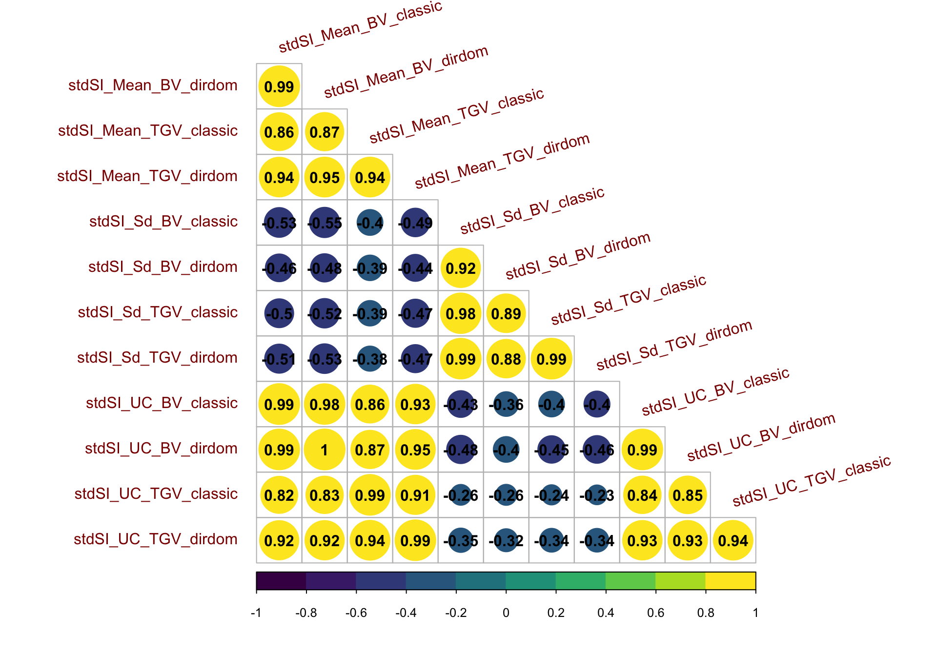
| Version | Author | Date |
|---|---|---|
| 6a10c30 | wolfemd | 2021-01-04 |
Figure S15: Correlation matrix for predictions on the BiofortSI
Figure S15: Correlation matrix for predictions on the BiofortSI. Heatmap of the correlations between predictions of mean, standard deviation, and usefulness in terms of BV and TGV, for both the classic and directional dominance model. Predictions were made for 47,083 possible pairwise crosses of 306 parents.
corMat_bio<-cor(forCorrMat[,grepl("biofortSI",colnames(forCorrMat))],use = 'pairwise.complete.obs')
corrplot::corrplot(corMat_bio, type = 'lower', col = viridis::viridis(n = 10), diag = F,addCoef.col = "black",
tl.srt = 15, tl.offset = 1,tl.col = 'darkred') 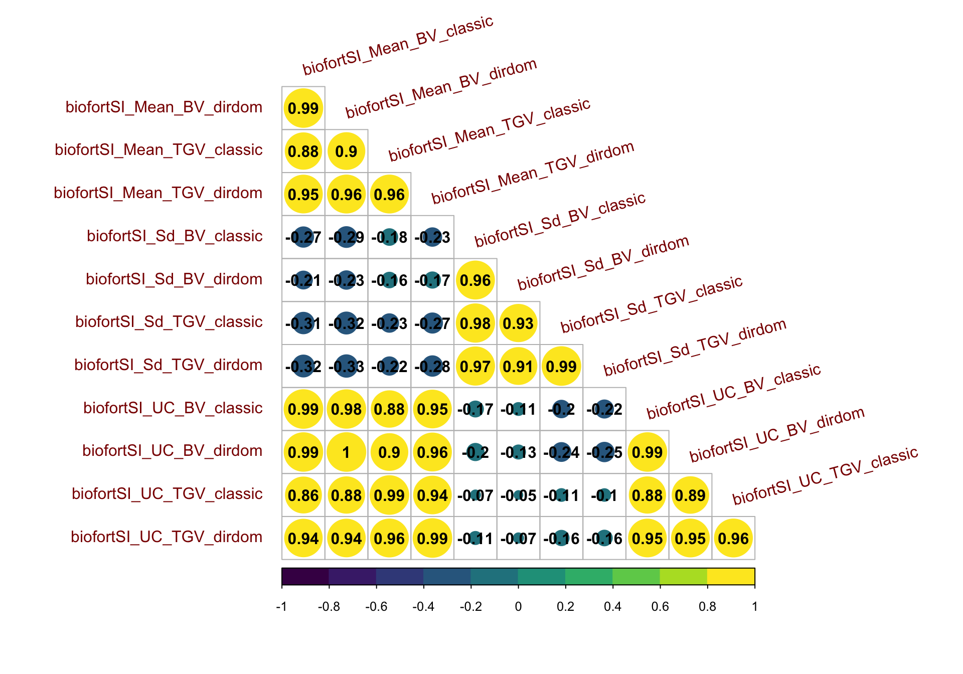
| Version | Author | Date |
|---|---|---|
| 6a10c30 | wolfemd | 2021-01-04 |
sessionInfo()R version 4.0.2 (2020-06-22)
Platform: x86_64-apple-darwin17.0 (64-bit)
Running under: macOS Catalina 10.15.7
Matrix products: default
BLAS: /Library/Frameworks/R.framework/Versions/4.0/Resources/lib/libRblas.dylib
LAPACK: /Library/Frameworks/R.framework/Versions/4.0/Resources/lib/libRlapack.dylib
locale:
[1] en_US.UTF-8/en_US.UTF-8/en_US.UTF-8/C/en_US.UTF-8/en_US.UTF-8
attached base packages:
[1] stats graphics grDevices utils datasets methods base
other attached packages:
[1] patchwork_1.1.1 magrittr_2.0.1 forcats_0.5.1 stringr_1.4.0
[5] dplyr_1.0.3 purrr_0.3.4 readr_1.4.0 tidyr_1.1.2
[9] tibble_3.0.6 ggplot2_3.3.3 tidyverse_1.3.0
loaded via a namespace (and not attached):
[1] Rcpp_1.0.6 lubridate_1.7.9.2 here_1.0.1 ps_1.5.0
[5] assertthat_0.2.1 rprojroot_2.0.2 digest_0.6.27 R6_2.5.0
[9] cellranger_1.1.0 backports_1.2.1 reprex_1.0.0 evaluate_0.14
[13] httr_1.4.2 highr_0.8 pillar_1.4.7 rlang_0.4.10
[17] readxl_1.3.1 rstudioapi_0.13 whisker_0.4 rmarkdown_2.6
[21] textshaping_0.2.1 labeling_0.4.2 munsell_0.5.0 broom_0.7.4
[25] compiler_4.0.2 httpuv_1.5.5 modelr_0.1.8 xfun_0.20
[29] systemfonts_0.3.2 gridGraphics_0.5-1 pkgconfig_2.0.3 htmltools_0.5.1.1
[33] tidyselect_1.1.0 gridExtra_2.3 workflowr_1.6.2 viridisLite_0.3.0
[37] crayon_1.3.4 dbplyr_2.0.0 withr_2.4.1 later_1.1.0.1
[41] grid_4.0.2 jsonlite_1.7.2 gtable_0.3.0 lifecycle_0.2.0
[45] DBI_1.1.1 git2r_0.28.0 scales_1.1.1 cli_2.3.0
[49] stringi_1.5.3 farver_2.0.3 viridis_0.5.1 fs_1.5.0
[53] promises_1.1.1 xml2_1.3.2 ragg_0.4.1 ellipsis_0.3.1
[57] generics_0.1.0 vctrs_0.3.6 tools_4.0.2 glue_1.4.2
[61] hms_1.0.0 yaml_2.2.1 colorspace_2.0-0 corrplot_0.84
[65] rvest_0.3.6 knitr_1.31 haven_2.3.1