Motif Analysis
Steve Pederson
2022-05-25
Last updated: 2022-06-06
Checks: 7 0
Knit directory:
apocrine_signature_mdamb453/
This reproducible R Markdown analysis was created with workflowr (version 1.7.0). The Checks tab describes the reproducibility checks that were applied when the results were created. The Past versions tab lists the development history.
Great! Since the R Markdown file has been committed to the Git repository, you know the exact version of the code that produced these results.
Great job! The global environment was empty. Objects defined in the global environment can affect the analysis in your R Markdown file in unknown ways. For reproduciblity it’s best to always run the code in an empty environment.
The command set.seed(20220427) was run prior to running
the code in the R Markdown file. Setting a seed ensures that any results
that rely on randomness, e.g. subsampling or permutations, are
reproducible.
Great job! Recording the operating system, R version, and package versions is critical for reproducibility.
Nice! There were no cached chunks for this analysis, so you can be confident that you successfully produced the results during this run.
Great job! Using relative paths to the files within your workflowr project makes it easier to run your code on other machines.
Great! You are using Git for version control. Tracking code development and connecting the code version to the results is critical for reproducibility.
The results in this page were generated with repository version 8dde309. See the Past versions tab to see a history of the changes made to the R Markdown and HTML files.
Note that you need to be careful to ensure that all relevant files for
the analysis have been committed to Git prior to generating the results
(you can use wflow_publish or
wflow_git_commit). workflowr only checks the R Markdown
file, but you know if there are other scripts or data files that it
depends on. Below is the status of the Git repository when the results
were generated:
Ignored files:
    Ignored:    .Rhistory
    Ignored:    .Rproj.user/
    Ignored:    data/bigwig/

Untracked files:
    Untracked:  output/meme/
Note that any generated files, e.g. HTML, png, CSS, etc., are not included in this status report because it is ok for generated content to have uncommitted changes.
These are the previous versions of the repository in which changes were
made to the R Markdown (analysis/motif_analysis.Rmd) and
HTML (docs/motif_analysis.html) files. If you’ve configured
a remote Git repository (see ?wflow_git_remote), click on
the hyperlinks in the table below to view the files as they were in that
past version.
| File | Version | Author | Date | Message |
|---|---|---|---|---|
| Rmd | 8dde309 | Steve Pederson | 2022-06-06 | Updated motif analysis |
| html | 8dde309 | Steve Pederson | 2022-06-06 | Updated motif analysis |
| Rmd | e1088ac | Steve Pederson | 2022-06-03 | revised comparison |
| Rmd | 16615bf | Steve Pederson | 2022-05-28 | Finished motif analysis |
| html | 16615bf | Steve Pederson | 2022-05-28 | Finished motif analysis |
| Rmd | 1bf46f7 | Steve Pederson | 2022-05-27 | Added motifs distance plots |
| html | 1bf46f7 | Steve Pederson | 2022-05-27 | Added motifs distance plots |
| Rmd | 7cfa8e7 | Steve Pederson | 2022-05-26 | Added TOMTOM |
| html | 7cfa8e7 | Steve Pederson | 2022-05-26 | Added TOMTOM |
| Rmd | 8836090 | Steve Pederson | 2022-05-26 | Added motif centrality |
| html | 8836090 | Steve Pederson | 2022-05-26 | Added motif centrality |
Introduction
This step takes the peaks defined previously and
- Assesses motif enrichment for all ChIP targets within the peaks
- Detect additional binding motifs
As AR is only found bound in the presence of DHT, all peaks are taken using DHT-treatment as the reference condition.
library(memes)
library(universalmotif)
library(tidyverse)
library(plyranges)
library(extraChIPs)
library(rtracklayer)
library(magrittr)
library(BSgenome.Hsapiens.UCSC.hg19)
library(scales)
library(pander)
library(glue)
library(cowplot)
library(parallel)
library(gt)
library(parallel)
library(readxl)
library(UpSetR)
library(reactable)
library(htmltools)
library(multcomp)
options(meme_bin = "/opt/meme/bin/")
check_meme_install()
theme_set(theme_bw())
panderOptions("big.mark", ",")
n_cores <- 12getBestMatch <- function(x, subject, min.score = "80%", rc = TRUE, ...) {
pwm <- NULL
if (is.matrix(x)) pwm <- x
if (is(x, "universalmotif")) pwm <- x@motif
stopifnot(!is.null(pwm))
stopifnot(is(subject, "XStringViews"))
matches <- matchPWM(
pwm, subject, min.score = min.score, with.score = TRUE, ...
)
df <- as.data.frame(matches)
df$score <- mcols(matches)$score
df$strand <- "+"
if (rc) {
rc_matches <- matchPWM(
reverseComplement(pwm), subject ,
min.score = min.score, with.score = TRUE,
...
)
rc_df <- as.data.frame(rc_matches)
rc_df$score <- mcols(rc_matches)$score
rc_df$strand <- "-"
df <- bind_rows(df, rc_df)
}
grp_cols <- c("start", "end", "width", "seq", "score")
grp_df <- group_by(df, !!!syms(grp_cols))
summ_df <- summarise(
grp_df, strand = paste(strand, collapse = " "), .groups= "drop"
)
summ_df$strand <- str_replace_all(summ_df$strand, ". .", "*")
summ_df$strand <- factor(summ_df$strand, levels = c("+", "-", "*"))
summ_df$view <- findInterval(summ_df$start, start(subject))
summ_df <- arrange(summ_df, view, desc(score))
best_df <- distinct(summ_df, view, .keep_all = TRUE)
best_df <- mutate(
best_df,
start_in_view = start - start(subject)[view] + 1,
end_in_view = start_in_view + width
)
## This will only be added if the views have names
best_df$view_name <- names(subject[best_df$view])
best_df
}
bar_style <- function(width = 1, fill = "#e6e6e6", height = "75%", align = c("left", "right"), color = NULL) {
align <- match.arg(align)
if (align == "left") {
position <- paste0(width * 100, "%")
image <- sprintf("linear-gradient(90deg, %1$s %2$s, transparent %2$s)", fill, position)
} else {
position <- paste0(100 - width * 100, "%")
image <- sprintf("linear-gradient(90deg, transparent %1$s, %2$s %1$s)", position, fill)
}
list(
backgroundImage = image,
backgroundSize = paste("100%", height),
backgroundRepeat = "no-repeat",
backgroundPosition = "center",
color = color
)
}hg19 <- BSgenome.Hsapiens.UCSC.hg19
sq19 <- seqinfo(hg19)all_gr <- here::here("data", "annotations", "all_gr.rds") %>%
read_rds() %>%
lapply(
function(x) {
seqinfo(x) <- sq19
x
}
)
counts <- here::here("data", "rnaseq", "counts.out.gz") %>%
read_tsv(skip = 1) %>%
dplyr::select(Geneid, ends_with("bam")) %>%
dplyr::rename(gene_id = Geneid)
detected <- all_gr$gene %>%
as_tibble() %>%
distinct(gene_id, gene_name) %>%
left_join(counts) %>%
pivot_longer(
cols = ends_with("bam"), names_to = "sample", values_to = "counts"
) %>%
mutate(detected = counts > 0) %>%
group_by(gene_id, gene_name) %>%
summarise(detected = mean(detected) > 0.25, .groups = "drop") %>%
dplyr::filter(detected) %>%
dplyr::select(starts_with("gene"))Pre-existing RNA-seq data was again loaded and the set of 21,173 detected genes was defined as those with \(\geq 1\) aligned read in at least 25% of samples. This dataset represented the DHT response in MDA-MB-453 cells, however, given the existence of both Vehicle and DHT conditions, represents a good representative measure of the polyadenylated components of the transcriptome.
features <- here::here("data", "h3k27ac") %>%
  list.files(full.names = TRUE, pattern = "bed$") %>%
  sapply(import.bed, seqinfo = sq19) %>%
  lapply(granges) %>%
  setNames(basename(names(.))) %>%
  setNames(str_remove_all(names(.), "s.bed")) %>%
  GRangesList() %>%
  unlist() %>%
  names_to_column("feature") %>%
  sort()
The set of H3K27ac-defined features was again used as a marker of regulatory activity, with 16,544 and 15,286 regions defined as enhancers or promoters respectively.
uniprot_to_ensg <- here::here("data", "external", "uniprot_to_ensg.txt.gz") %>%
  read_tsv(col_names = c("uniprot_id", "protein", "gene_id")) %>%
  mutate(
    gene_id = lapply(gene_id, str_split, pattern = "; ") %>%
      lapply(unlist)
  ) %>%
  unnest(gene_id) %>%
  mutate(gene_id = str_replace_all(gene_id, "(ENSG[0-9]+)\\..*", "\\1")) %>%
  left_join(
    as_tibble(all_gr$gene) %>%
      dplyr::select(gene_id, gene_name)
  ) %>%
  dplyr::filter(!is.na(gene_id)) %>%
  dplyr::select(-protein)
rime_detected <- here::here("data", "external", "MDA-MB-453_RIME_processed.xlsx") %>%
  read_excel() %>%
  dplyr::select(-starts_with("AVG"), -ends_with("Coverage2"), -contains("delta")) %>%
  pivot_longer(cols = contains("_")) %>%
  separate(name, c("sample", "measure"), sep = "_", extra = "merge") %>%
  mutate(
    IP = str_remove(sample, "[0-9]$"),
    replicate = str_extract(sample, "[0-9]$"),
    measure = paste(measure, IP, sep = "_")
  ) %>%
  pivot_wider(
    names_from = "measure", values_from = "value",
    id_cols = c("Accession", "Description", "Protein", "replicate")
  ) %>%
  mutate(
    logfc_cov = log2(Coverage_AR + 1) - log2(Coverage_IgG + 1),
    logfc_peptides = log2(Unique_peptides_AR + 1) - log2(Unique_peptides_IgG + 1)
  ) %>%
  dplyr::filter(logfc_cov > 0) %>%
  group_by(Accession, Description, Protein) %>%
  summarise(
    n_detected = dplyr::n(),
    mn_logfc_coverage = mean(logfc_cov),
    mn_coverage_AR = mean(Coverage_AR),
    mn_coverage_IgG = mean(Coverage_IgG),
    mn_peptides_AR = mean(Unique_peptides_AR),
    mn_peptides_IgG = mean(Unique_peptides_IgG),
    .groups = "drop"
  ) %>%
  dplyr::filter(n_detected > 1) %>%
  arrange(desc(mn_logfc_coverage)) %>%
  left_join(uniprot_to_ensg, by = c("Accession" = "uniprot_id")) %>%
  dplyr::select(
    Accession, Description, Protein, starts_with("gene"), everything()
  ) %>%
  dplyr::filter(!is.na(gene_name))
AR-RIME data for MDA-MB-453 cells was also used, with protein to
transcript ID mappings performed using the mappings obtained using the
following bash command
curl https://ftp.uniprot.org/pub/databases/uniprot/current_release/knowledgebase/idmapping/by_organism/HUMAN_9606_idmapping_selected.tab.gz |\
  zcat |\
  cut -f1-2,19 |\
  gzip -c > data/external/uniprot_to_ensg.txt.gz
For RIME data the criteria for detection within a sample was simply defined as the coverage being greater when using AR as the IP-target, than when using IgG as the IP-target. Any genes with no gene_name associated (i.e. only an Ensembl Gene ID) were also excluded. Under this approach, 241 proteins were considered as detected in \(>2\) of 3 samples and were retained for inclusion with motif analysis. When further comparing to the RNA-Seq data only KRT9 was found in the RIME data without supporting RNA evidence.
meme_db <- here::here("data", "external", "JASPAR2022_CORE_Hsapiens.meme") %>%
  read_meme() %>%
  to_df() %>%
  as_tibble() %>%
  mutate(
    across(everything(), vctrs::vec_proxy),
    altname = str_remove(altname, "MA[0-9]+\\.[0-9]*\\."),
    organism = "Homo sapiens"
  )
meme_altname <- setNames(meme_db$altname, meme_db$name)
meme_db_detected <- meme_db %>%
  mutate(
    gene_name = str_split(altname, pattern = "::", n = 2)
  ) %>%
  dplyr::filter(
    vapply(
      gene_name,
      function(x) all(x %in% detected$gene_name),
      logical(1)
    )
  )
meme_info <- meme_db_detected %>%
  mutate(motif_length = vapply(motif, function(x){ncol(x@motif)}, integer(1))) %>%
  dplyr::select(name, altname, icscore, motif_length)
The motif database was initially defined as all 727 CORE motifs found in Homo sapiens, as contained in JASPAR2022. In order to minimise irrelevant results, only the 465 motifs associated with a **detected as an AR interacting were then retained.
dht_peaks <- here::here("data", "peaks") %>%
  list.files(recursive = TRUE, pattern = "oracle", full.names = TRUE) %>%
  sapply(read_rds, simplify = FALSE) %>%
  lapply(function(x) x[["DHT"]]) %>%
  lapply(setNames, nm = c()) %>%
  setNames(str_extract_all(names(.), "AR|FOXA1|GATA3|TFAP2B")) %>%
  lapply(
    function(x) {
      seqinfo(x) <- sq19
      x
    }
  )
targets <- names(dht_peaks)
dht_consensus <- dht_peaks %>%
  lapply(granges) %>%
  GRangesList() %>%
  unlist() %>%
  reduce() %>%
  mutate(
    AR = overlapsAny(., dht_peaks$AR),
    FOXA1 = overlapsAny(., dht_peaks$FOXA1),
    GATA3 = overlapsAny(., dht_peaks$GATA3),
    TFAP2B = overlapsAny(., dht_peaks$TFAP2B),
    promoter = bestOverlap(., features, var = "feature", missing = "None") == "promoter",
    enhancer = bestOverlap(., features, var = "feature", missing = "None") == "enhancer",
    H3K27ac = promoter | enhancer
  )
a <- dht_peaks %>%
lapply(mutate, w = width) %>%
lapply(as_tibble) %>%
bind_rows(.id = "target") %>%
ggplot(aes(w, stat(density), colour = target)) +
geom_density() +
scale_x_log10(breaks = c(100, 300, 600, 1e3, 2e3, 3e3), labels = comma) +
labs(
x = "Peak Width (bp)", y = "Density", colour = "Target"
)
b <- dht_peaks %>%
lapply(mutate, w = width) %>%
lapply(as_tibble) %>%
bind_rows(.id = "target") %>%
mutate(skew = 0.5 - peak / w) %>%
ggplot(aes(skew, stat(density), colour = target)) +
geom_density() +
scale_x_continuous(labels = percent) +
labs(
x = "% Width Between Peak Summit and Peak Centre",
y = "Density",
colour = "ChIP Target"
)
plot_grid(
a + theme(legend.position = "none"),
b + theme(legend.position = "none"),
get_legend(b),
rel_widths = c(1, 1, 0.2), nrow = 1,
labels = c("A", "B")
)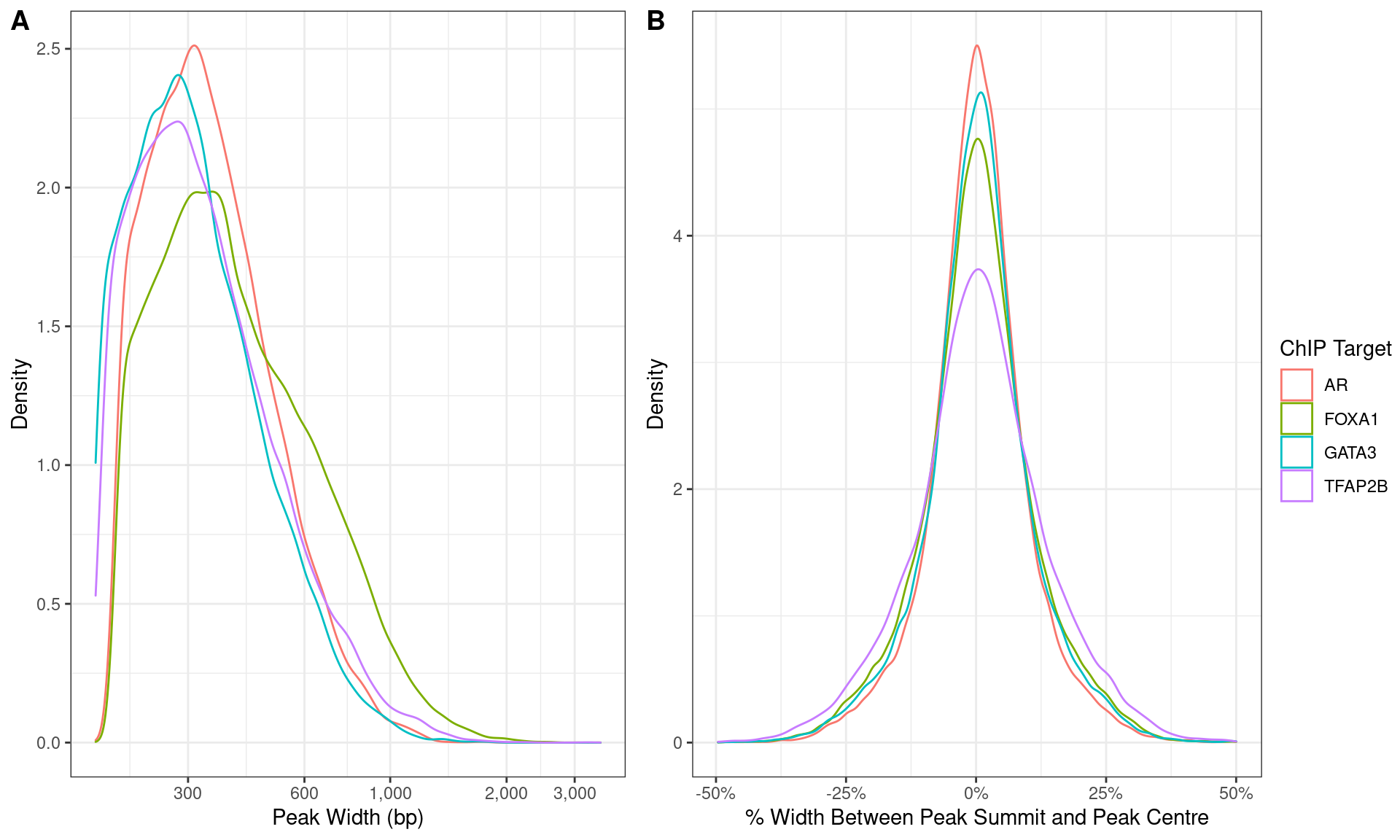
Distributions of A) peak width and B) summit location with peaks.
| Version | Author | Date |
|---|---|---|
| 8836090 | Steve Pederson | 2022-05-26 |
Analysis of Motif Enrichment (AME)
grl_by_targets <- dht_consensus %>%
  as_tibble() %>%
  pivot_longer(
    all_of(targets), names_to = "target", values_to = "detected"
  ) %>%
  dplyr::filter(detected) %>%
  group_by(range, H3K27ac) %>%
  summarise(
    targets = paste(sort(target), collapse = " "),
    .groups = "drop"
  ) %>%
  colToRanges(var = "range", seqinfo = sq19) %>%
  sort() %>%
  splitAsList(.$targets)
Union ranges were grouped by the combination of detected AR, FOXA1, GATA3 and TFAP2B binding, then sequences obtained corresponding to each union range.
grl_by_targets %>%
  lapply(
    function(x) {
      tibble(
        `N Sites` = length(x),
        `% H3K27ac` = mean(x$H3K27ac),
        `Median Width` = floor(median(width(x)))
      )
    }
  ) %>%
  bind_rows(.id = "Targets") %>%
  mutate(
    `N Targets` = str_count(Targets, " ") + 1,
    `% H3K27ac` = percent(`% H3K27ac`, 0.1)
  ) %>%
  dplyr::select(contains("Targets"), everything()) %>%
  arrange(`N Targets`, Targets) %>%
  pander(
    justify = "lrrrr",
    caption = "Summary of union ranges and which combinations of the targets were detected."
)| Targets | N Targets | N Sites | % H3K27ac | Median Width |
|---|---|---|---|---|
| AR | 1 | 395 | 13.9% | 241 |
| FOXA1 | 1 | 59,404 | 12.8% | 319 |
| GATA3 | 1 | 4,284 | 19.6% | 234 |
| TFAP2B | 1 | 6,655 | 80.1% | 301 |
| AR FOXA1 | 2 | 3,543 | 17.8% | 505 |
| AR GATA3 | 2 | 158 | 16.5% | 310 |
| AR TFAP2B | 2 | 135 | 55.6% | 414 |
| FOXA1 GATA3 | 2 | 9,760 | 18.1% | 479 |
| FOXA1 TFAP2B | 2 | 3,849 | 64.6% | 513 |
| GATA3 TFAP2B | 2 | 396 | 60.6% | 368 |
| AR FOXA1 GATA3 | 3 | 6,518 | 25.2% | 683 |
| AR FOXA1 TFAP2B | 3 | 1,786 | 62.9% | 639 |
| AR GATA3 TFAP2B | 3 | 61 | 55.7% | 419 |
| FOXA1 GATA3 TFAP2B | 3 | 1,441 | 52.0% | 575 |
| AR FOXA1 GATA3 TFAP2B | 4 | 6,336 | 58.2% | 814 |
seq_by_targets <- grl_by_targets %>%
  lapply(function(x) split(x, x$H3K27ac)) %>%
  lapply(GRangesList) %>%
  lapply(get_sequence, genome = hg19)

## All bound sites
rds_ame_by_targets <- here::here("output", "ame_by_targets.rds")
if (!file.exists(rds_ame_by_targets)) {
  ame_by_targets <- seq_by_targets %>%
    lapply(unlist) %>%
    mclapply(
      runAme,
      database = to_list(meme_db_detected),
      mc.cores = min(n_cores, length(.))
    )
  write_rds(ame_by_targets, rds_ame_by_targets, compress = "gz")
} else {
  ame_by_targets <- read_rds(rds_ame_by_targets)
}

## Only sites marked as active by H3K27ac
rds_ame_by_targets_active <- here::here("output", "ame_by_targets_active.rds")
if (!file.exists(rds_ame_by_targets_active)) {
  ame_by_targets_active <- seq_by_targets %>%
    lapply(function(x) x[["TRUE"]]) %>%
    mclapply(
      runAme,
      database = to_list(meme_db_detected),
      mc.cores = min(n_cores, length(.))
    )
  write_rds(ame_by_targets_active, rds_ame_by_targets_active, compress = "gz")
} else {
  ame_by_targets_active <- read_rds(rds_ame_by_targets_active)
}

## Compare the active and inactive sites for each set of targets
rds_ame_active_vs_inactive <- here::here("output", "ame_active_vs_inactive.rds")
if (!file.exists(rds_ame_active_vs_inactive)) {
  ame_active_vs_inactive <- seq_by_targets %>%
    mclapply(
      function(x) {
        runAme(x[["TRUE"]], x[["FALSE"]], database = to_list(meme_db_detected))
      },
      mc.cores = min(n_cores, length(.))
    )
  write_rds(ame_active_vs_inactive, rds_ame_active_vs_inactive, compress = "gz")
} else {
  ame_active_vs_inactive <- read_rds(rds_ame_active_vs_inactive)
}

## Compare the inactive and active sites for each set of targets
rds_ame_inactive_vs_active <- here::here("output", "ame_inactive_vs_active.rds")
if (!file.exists(rds_ame_inactive_vs_active)) {
  ame_inactive_vs_active <- seq_by_targets %>%
    mclapply(
      function(x) {
        runAme(x[["FALSE"]], x[["TRUE"]], database = to_list(meme_db_detected))
      },
      mc.cores = min(n_cores, length(.))
    )
  write_rds(ame_inactive_vs_active, rds_ame_inactive_vs_active, compress = "gz")
} else {
  ame_inactive_vs_active <- read_rds(rds_ame_inactive_vs_active)
}
AME from the meme-suite was then run on each sequence to detect the presence of motifs associated with each target within each set of sequences. Under this approach the optimal score is estimated for considering a PWM match to be a true positive. Matches above this value are classed as true positives, whilst those below are considered as false positives. Significance is determined using using Fisher’s Exact Test against the set of control sequences, which are either shuffled input sequences, or a discrete set provided. Adjusted p-values are determined within each motif based on resampling, with the e-values representing a Bonferroni adjustment of the within-motif adjusted p-values.
Motif enrichment inevitably produces hits to highly-related motifs For unsupervised enrichment, the following strategy was used to aid interpretation
- Find enriched motifs
- Calculate similarity of enriched motifs as a correlation matrix
- Reduce correlations < 0.9 to zero
- Converted to a distance matrix for clustering
- Cluster the motifs using
hclustand a height of 0.9 - Create a consensus motif for all motifs in the cluster
- Report enriched consensus motifs for simpler interpretation
Enrichment Of ChIP Target Motifs
plot_grid(
  plot_grid(
    plotlist = lapply(
      meme_db_detected %>%
        dplyr::filter(altname %in% targets) %>%
        arrange(altname) %>%
        dplyr::filter(altname != "TFAP2B") %>%
        to_list() %>%
        lapply(
          function(x){
            x@name <- paste0(
              x@name, " (", x@altname, ")"
            )
            x
          }
        ),
      function(x) {
        view_motifs(x) +
          ggtitle(x@name) +
          theme(plot.title = element_text(hjust = 0.5, size = 11))
      }
    ),
    ncol = 1
  ),
  plot_grid(
    meme_db_detected %>%
      dplyr::filter(altname == "TFAP2B") %>%
      to_list() %>%
      lapply(
          function(x){
            x@name <- paste0(
              x@name, " (", x@altname, ")"
            )
            x
          }
      ) %>%
      view_motifs() +
      theme(plot.title = element_text(hjust = 0.5, size = 9))
  ),
  ncol = 2
)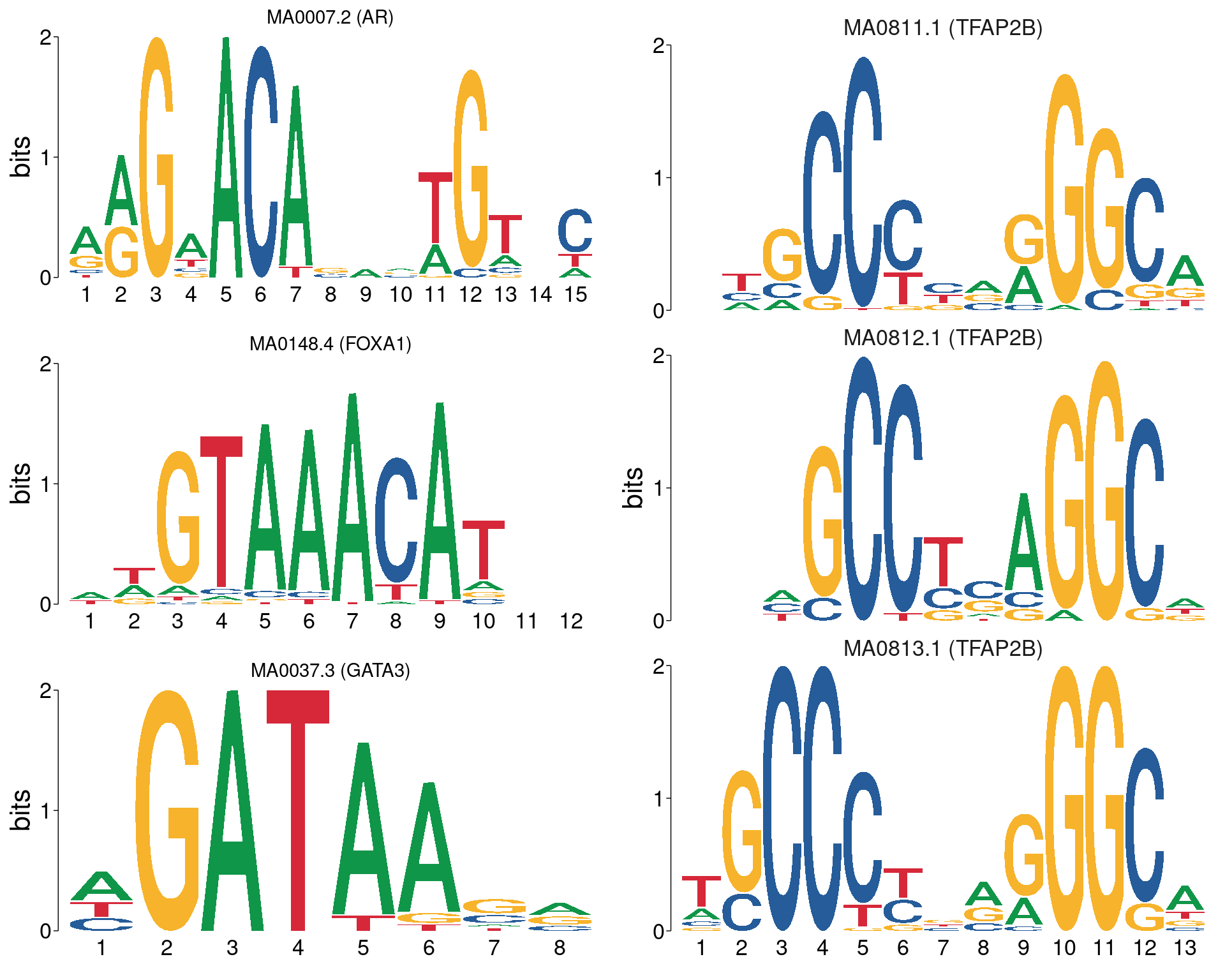
All motifs matching the set of ChIP targets. AR, FOXA1 and GATA3 are not aligned with each other, whilst all TFAP2B motifs are shown using the best alignment to each other.
All Sequences
AME was used to assess enrichment of motifs within the sequences derived from each combination of ChIP targets. Enrichment was considered relative to shuffled sequences as the control set, with AME only returning matches considered to be statistically significant.
ame_by_targets %>%
  bind_rows(.id = "targets") %>%
  dplyr::filter(motif_alt_id %in% globalenv()$targets) %>%
  mutate(
    motif_id = as.factor(motif_id),
    targets = as.factor(targets),
    TFAP2B = ifelse(
      str_detect(targets, "TFAP2B"), "TFAP2B", "No TFAP2B"
    )
  ) %>%
  plot_ame_heatmap(
    id = motif_id,
    value = tp_percent,
    group = fct_rev(targets)
  ) +
  geom_label(
    aes(label = percent(tp_percent/100, 0.1)),
    size = 3.5,
    show.legend = FALSE
  ) +
  facet_grid(TFAP2B ~ motif_alt_id, scales = "free", space = "free") +
  scale_x_discrete(expand = expansion(c(0, 0))) +
  scale_y_discrete(expand = expansion(c(0, 0))) +
  labs(
    x = "Detected Motif",
    y = "Detected ChIP Targets",
    fill = expression(widehat("TP%"))
  ) +
  theme(
    axis.text.x = element_text(angle = 0, hjust = 0.5, size = 10),
    axis.text.y = element_text(angle = 0, hjust = 1, size = 10),
    panel.grid = element_blank()
  )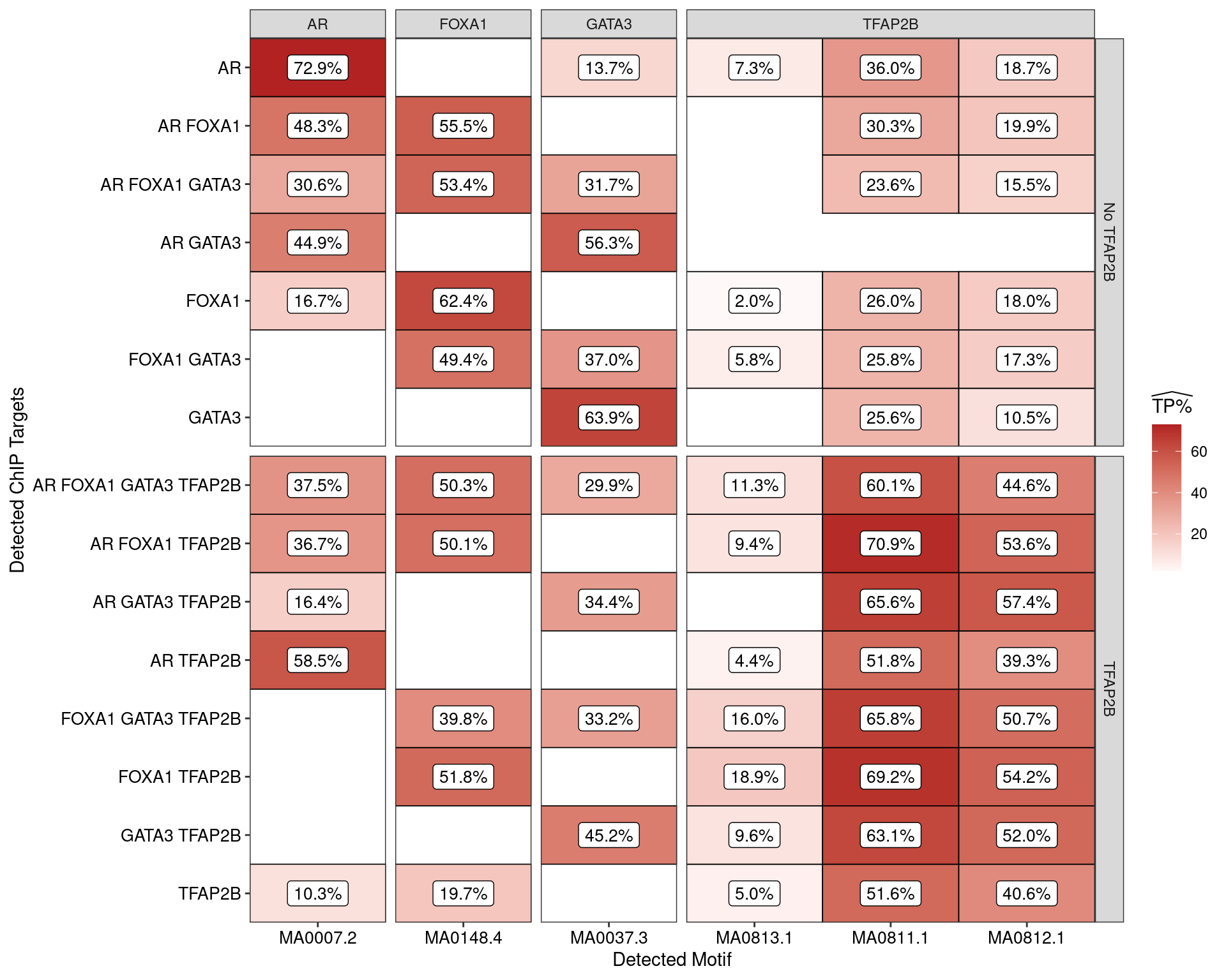
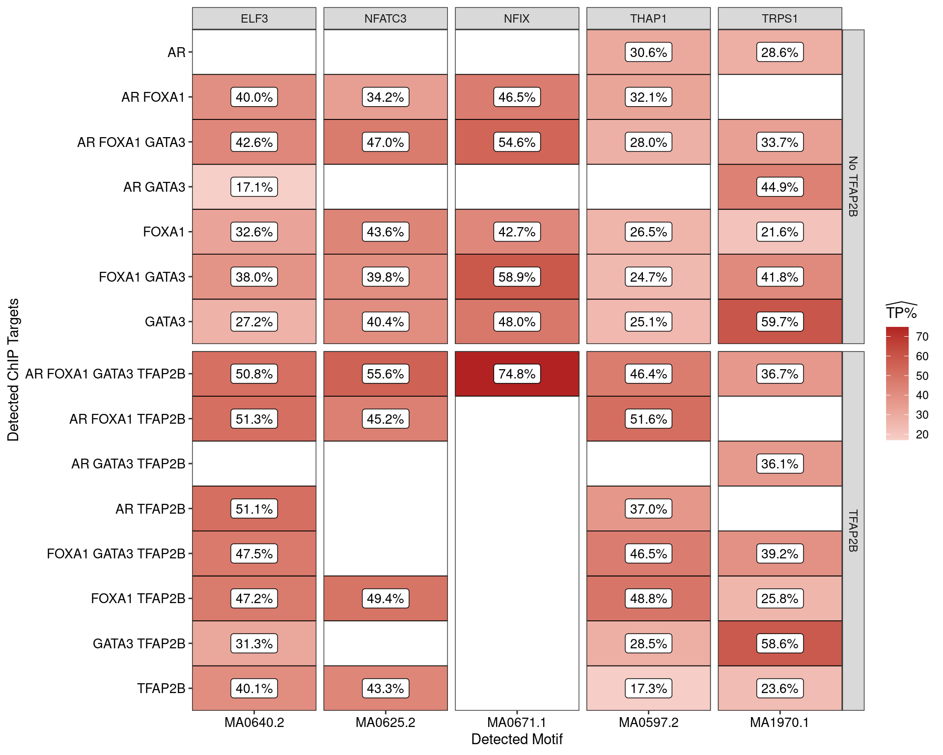
Estimated percentage of true positive matches to all binding motifs associated with each ChIP target within all sequences. Only motifs considered to be enriched are shown, such that missing values are able to be confidently assumed as not enriched for the motif. All provide supporting evidence for direct binding of each target to it’s motif.
H3K27ac-Associated Sequences
Restricting the test for motif enrichment to all combinations of ChIP targets which overlap an active H3K27ac peak, similar patterns were observed. Of possible note is reduced enrichment for TFAP2\(\beta\) motifs amongst the sites where TFAP2\(\beta\) was not observed.
The set of H3K27-associated peaks where AR, GATA3 and TFAP2\(\beta\) were found in combination were notably enriched for one specific TFAP2$ motif (MA0812) to the exclusion of others suggesting that FOXA1 independent formation of the regulatory complex may have a distinct mechanism. In conjunction with the increased occurrence of this motif, this set of peaks also contained the lowest enrichment for AR motifs amongst the AR-associated peaks.
Another clear association between the presence of FOXA1 and possible increased enrichment for the MA0811.1 TFAP2\(\beta\) motif may also be of interest.
ame_by_targets_active %>%
  bind_rows(.id = "targets") %>%
  dplyr::filter(motif_alt_id %in% globalenv()$targets) %>%
  mutate(
    motif_id = as.factor(motif_id),
    targets = as.factor(targets),
    TFAP2B = ifelse(
      str_detect(targets, "TFAP2B"), "TFAP2B", "No TFAP2B"
    )
  ) %>%
  plot_ame_heatmap(
    id = motif_id,
    value = tp_percent,
    group = fct_rev(targets)
  ) +
  geom_label(
    aes(label = percent(tp_percent/100, 0.1)),
    size = 3.5,
    show.legend = FALSE
  ) +
  facet_grid(TFAP2B ~ motif_alt_id, scales = "free", space = "free") +
  scale_x_discrete(expand = expansion(c(0, 0))) +
  scale_y_discrete(expand = expansion(c(0, 0))) +
  labs(
    x = "Detected Motif",
    y = "Detected ChIP Targets",
    fill = expression(widehat("TP%"))
  ) +
  theme(
    axis.text.x = element_text(angle = 0, hjust = 0.5, size = 10),
    axis.text.y = element_text(angle = 0, hjust = 1, size = 10),
    panel.grid = element_blank()
  )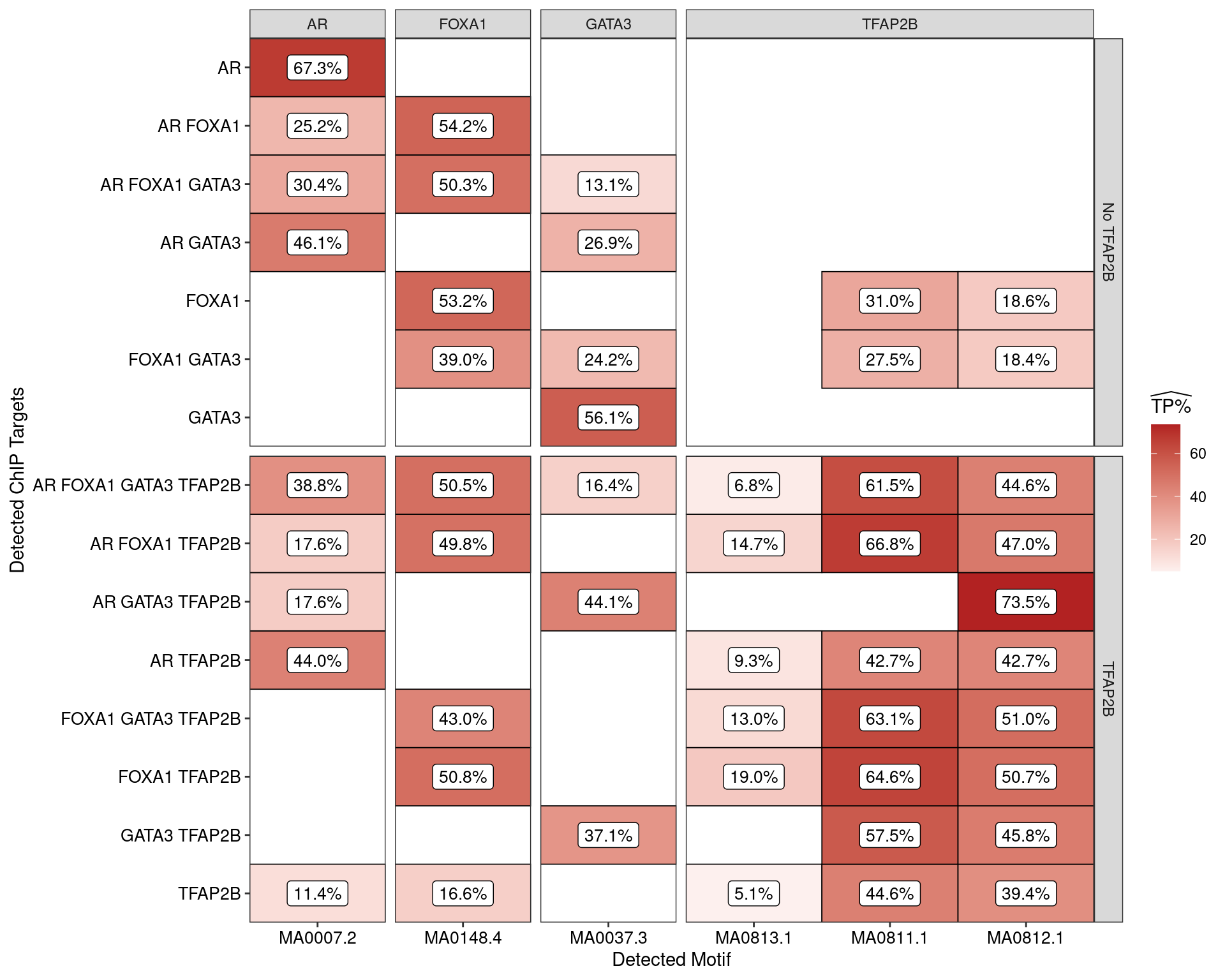
Estimated percentage of true positive matches to all binding motifs associated with each ChIP target, restricting sequences to those marked by overlapping H3K27ac signal. Only motif considered to be enriched are shown, such that missing values are able to be confidently assumed as not enriched for the motif. All provide supporting evidence for direct binding of each target to it’s motif. Interestingly FOXA1 in combination with TFAP2B appears to favour the motif MA0811.1, whilst AR and GATA3 in combination with TFAP2B appears to favour MA0812.1
| Version | Author | Date |
|---|---|---|
| 8dde309 | Steve Pederson | 2022-06-06 |
Enrichment of Other Motifs
Motifs associated with any detected transcription factor besides the ChIP targets were also assessed for enrichment. Motifs which matched GATA[0-9], Forkhead (FOX[A-Z][0-9]) or TFAP2[A-Z] were omitted due to the high-level of motif redundancy and these being likely to represent the ChIP target, instead of an additional protein. Given that an extremely large number of motifs were found, only those found in >50% of sites in at least one group of ChIP targets were retained
All Sequences
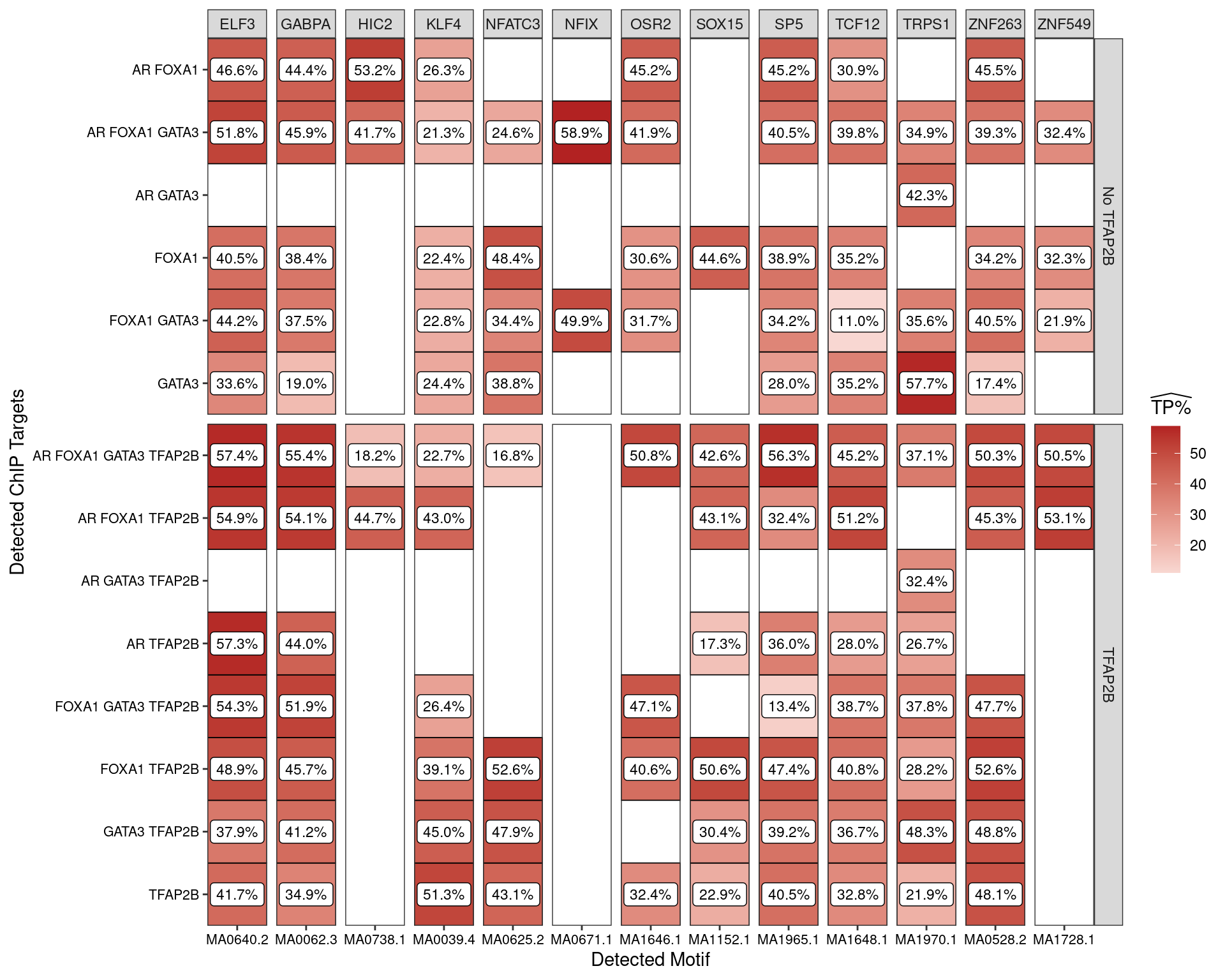
The set of motifs associated with detectable genes (using RNA) was tested for enrichment against all sequences from all combinations of ChIP target binding, using shuffled sequences as controls. Given that 375 motifs were considered to be enriched in at least one set of peaks, the plot below only shows those motifs which were found in >50% of sequences in one or more sets of peaks.
The NFIX binding motif was strongly associated with most sets of peaks which were not bound by TFAP2\(\beta\), particularly with FOXA1 in the absence of TFAP2\(\beta\). However, a very strong association with all four bound targets was also observed. Given the short (6nt) nature of this motif, this may be artefactual.
The TRPS1 motif was also found to be strongly enriched where GATA3 was bound, however, this motif bears a very strong resemblance to the GATA3 motif.
meme_db %>%
  dplyr::filter(str_detect(altname, "GATA3|TRPS1")) %>%
  to_list() %>%
  lapply(function(x) {x@name <- glue("{x@name}\n({x@altname})"); x}) %>%
  view_motifs(names.pos = "right")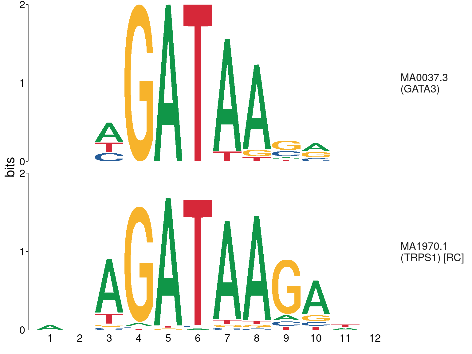
Comparison between GATA3 and TRPS1 motifs
| Version | Author | Date |
|---|---|---|
| 8dde309 | Steve Pederson | 2022-06-06 |
x <- ame_by_targets %>%
  bind_rows(.id = "targets") %>%
  dplyr::filter(
    !motif_alt_id %in% targets,
    !str_detect(motif_alt_id, "(GATA[0-9]|FOX[A-Z][0-9]|TFAP2[A-Z])"),
    tp_percent > 50
  ) %>%
  distinct(motif_id) %>%
  pull("motif_id")
cormat <- meme_db %>%
  dplyr::filter(name %in% x) %>%
  to_list() %>%
  compare_motifs()
cormat[cormat < 0.9] <- 0
cormat[is.na(cormat)] <- 0
cl <- as.dist(1 - cormat) %>%
  hclust() %>%
  cutree(h= 0.9)
ame_by_targets %>%
  bind_rows(.id = "targets") %>%
  dplyr::filter(motif_id %in% names(cl)) %>%
  mutate(
    cluster = cl[motif_id],
    motif_id = as.factor(motif_id),
    targets = as.factor(targets),
    TFAP2B = ifelse(
      str_detect(targets, "TFAP2B"), "TFAP2B", "No TFAP2B"
    )
  ) %>%
  group_by(cluster) %>%
  mutate(
    best_tp = max(tp_percent)
  ) %>%
  ungroup() %>%
  group_by(motif_id) %>%
  dplyr::filter(any(tp_percent == best_tp)) %>%
  ungroup() %>%
  plot_ame_heatmap(
    id = motif_id,
    value = tp_percent,
    group = fct_rev(targets)
  ) +
  geom_label(
    aes(label = percent(tp_percent/100, 0.1)),
    size = 3.5,
    show.legend = FALSE
  ) +
  facet_grid(TFAP2B ~ motif_alt_id, scales = "free", space = "free") +
  scale_x_discrete(expand = expansion(c(0, 0))) +
  scale_y_discrete(expand = expansion(c(0, 0))) +
  labs(
    x = "Detected Motif",
    y = "Detected ChIP Targets",
    fill = expression(widehat("TP%"))
  ) +
  theme(
    axis.text.x = element_text(angle = 0, hjust = 0.5, size = 10),
    axis.text.y = element_text(angle = 0, hjust = 1, size = 10),
    panel.grid = element_blank()
  )
Enriched motifs when analysing all sequences associated with one or more ChIP targets. Motifs are only shown if found in >50% of sequences from at least one set of peaks.
| Version | Author | Date |
|---|---|---|
| 8dde309 | Steve Pederson | 2022-06-06 |
H3K27ac Active Sequences
When restricting the peaks to being any ChIP-target binding peak associated with H3K27ac significantly more motifs were considered to be enriched.
Notably:
- NFIX enrichment was mostly lost, especially in the set of peaks associated with all four targets. Significance was retained for FOXA1 and GATA3 in combination, but only in the absence of TFAP2\(\beta\)
- HIC2 was enriched in all combinations where AR and FOXA1 were bound in combination. However, HIC2 was not found in combination with AR in the RIME dataset.
No other striking patterns were observed.
x <- ame_by_targets_active %>%
  bind_rows(.id = "targets") %>%
  dplyr::filter(
    !motif_alt_id %in% targets,
    !str_detect(motif_alt_id, "(GATA[0-9]|FOX[A-Z][0-9]|TFAP2[A-Z])"),
    tp_percent > 50
  ) %>%
  distinct(motif_id) %>%
  pull("motif_id")
cormat <- meme_db %>%
  dplyr::filter(name %in% x) %>%
  to_list() %>%
  compare_motifs()
cormat[cormat < 0.9] <- 0
cormat[is.na(cormat)] <- 0
cl <- as.dist(1 - cormat) %>%
  hclust() %>%
  cutree(h= 0.9)
ame_by_targets_active %>%
  bind_rows(.id = "targets") %>%
  dplyr::filter(motif_id %in% names(cl)) %>%
  mutate(
    cluster = cl[motif_id],
    motif_id = as.factor(motif_id),
    targets = as.factor(targets),
    TFAP2B = ifelse(
      str_detect(targets, "TFAP2B"), "TFAP2B", "No TFAP2B"
    )
  ) %>%
  group_by(cluster) %>%
  mutate(
    best_tp = max(tp_percent)
  ) %>%
  ungroup() %>%
  group_by(motif_id) %>%
  dplyr::filter(any(tp_percent == best_tp)) %>%
  ungroup() %>%
  plot_ame_heatmap(
    id = motif_id,
    value = tp_percent,
    group = fct_rev(targets)
  ) +
  geom_label(
    aes(label = percent(tp_percent/100, 0.1)),
    size = 3,
    show.legend = FALSE
  ) +
  facet_grid(TFAP2B ~ motif_alt_id, scales = "free", space = "free") +
  scale_x_discrete(expand = expansion(c(0, 0))) +
  scale_y_discrete(expand = expansion(c(0, 0))) +
  labs(
    x = "Detected Motif",
    y = "Detected ChIP Targets",
    fill = expression(widehat("TP%"))
  ) +
  theme(
    axis.text.x = element_text(angle = 0, hjust = 0.5, size = 8),
    axis.text.y = element_text(angle = 0, hjust = 1, size = 8),
    panel.grid = element_blank()
  )
Enriched motifs when analysing all sequences associated with one or more ChIP targets and which overlap an H3K27ac peak. Motifs are only shown if found in >50% of sequences from at least one set of peaks.
| Version | Author | Date |
|---|---|---|
| 8dde309 | Steve Pederson | 2022-06-06 |
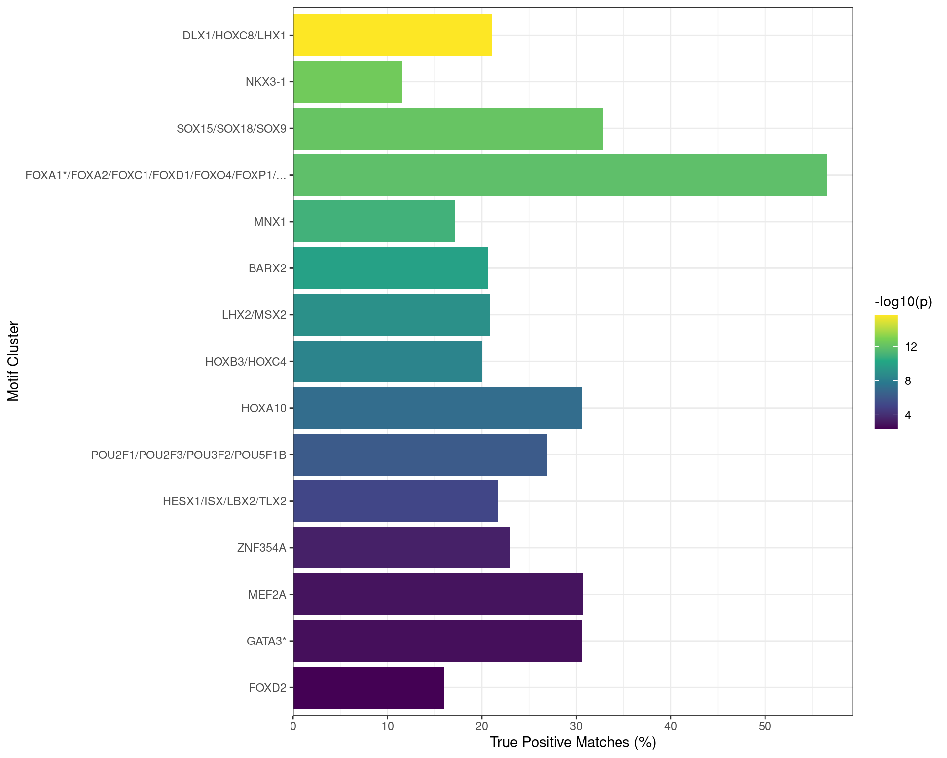
H3K27ac Active Vs Inactive
In order to ascertain whether any co-factors are playing a role in active vs inactive regulatory regions, the set of sequences associated with binding of all four targets were compared to each other, based on H3K27ac overlap as the marker of an active regulatory region. Enriched motifs were those with an \(E\)-value < 0.01 and with a True Positive match in > 10% of sequences.
Due to the high-levels of similarity between identified motifs, enriched motifs were clustered by:
- Finding the pairwise correlations
- Setting all pairwise correlations < 0.8 to zero
- Using hierarchical clustering to cluster those with retained correlations
For each motif cluster the values used for visualisation were the lowest \(E\)-value within the cluster and the high estimate of True Positive matches.
x <- ame_active_vs_inactive$`AR FOXA1 GATA3 TFAP2B` %>%
  dplyr::filter(
    evalue < 0.01,
    tp_percent > 10
  ) %>%
  distinct(motif_id) %>%
  pull("motif_id")
cormat <- meme_db %>%
  dplyr::filter(name %in% x) %>%
  to_list() %>%
  compare_motifs()
cormat[cormat < 0.80] <- 0
cormat[is.na(cormat)] <- 0
cl_active_vs_inactive <- as.dist(1 - cormat) %>%
  hclust() %>%
  cutree(h= 0.9)
ame_active_vs_inactive$`AR FOXA1 GATA3 TFAP2B` %>%
  dplyr::filter(motif_id %in% names(cl_active_vs_inactive)) %>%
  mutate(
    cluster = cl_active_vs_inactive[motif_id],
    in_rime = motif_alt_id %in% rime_detected$gene_name,
    motif_alt_id = ifelse(in_rime, paste0(motif_alt_id, "*"), motif_alt_id)
  ) %>%
  group_by(cluster) %>%
  summarise(
    tp_percent = max(tp_percent),
    p = min(evalue),
    id = motif_alt_id %>%
      unique %>%
      sort() %>%
      paste(collapse = "/")
  ) %>%
  arrange(p) %>%
  mutate(
    id = str_trunc(id, width = 40) %>% fct_inorder()
  ) %>%
  ggplot(
    aes(tp_percent, fct_rev(id), fill = -log10(p))
  ) +
  geom_col() +
  scale_x_continuous(expand = expansion(c(0, 0.05))) +
  scale_fill_viridis_c() +
  labs(
    x = "True Positive Matches (%)",
    y = "Motif Cluster"
  )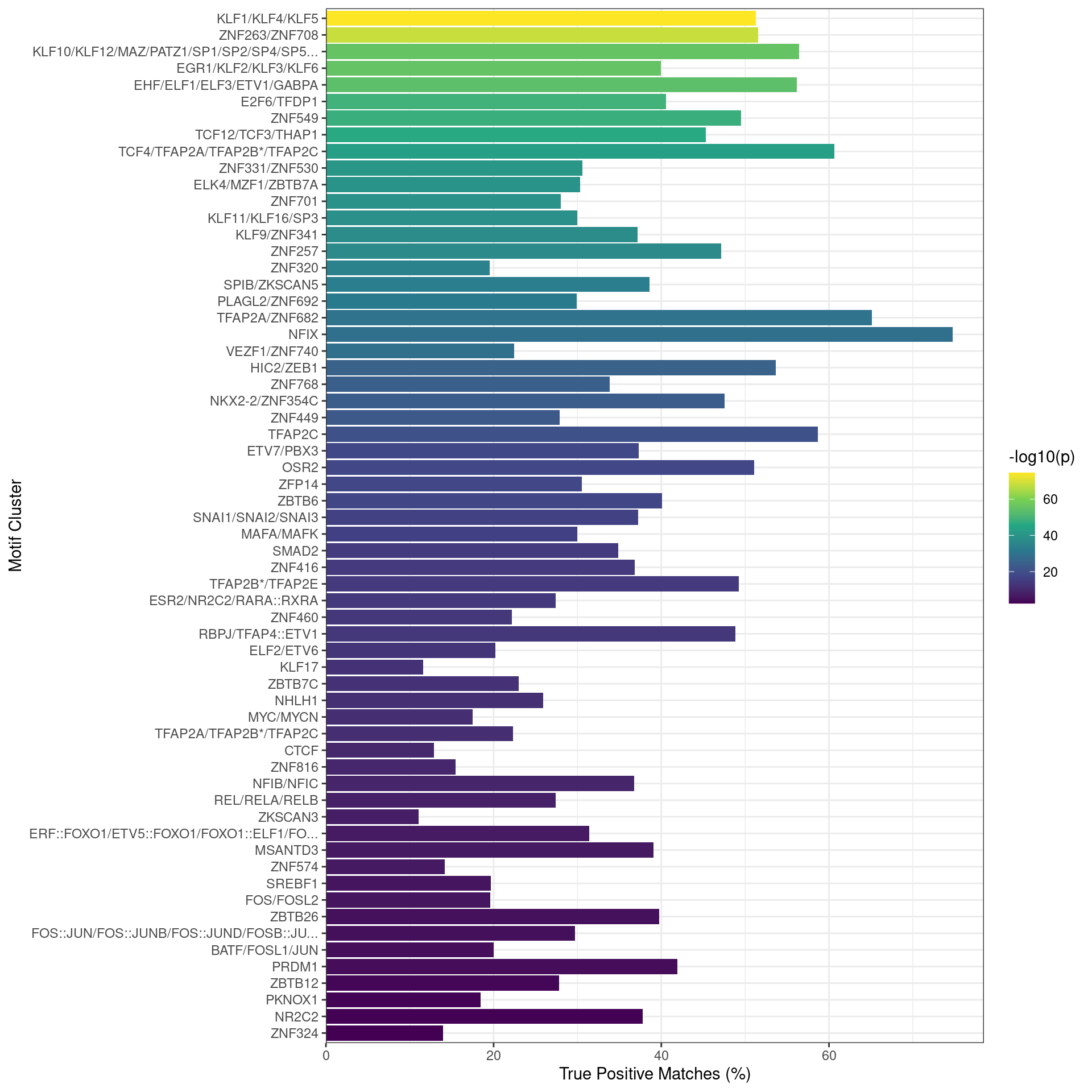
Motifs found enriched when comparing sequences from peaks overlapping an active H3K27ac regulatory region, with those from peaks not overlapping an H3K27ac-marked region. Motifs were clustered as described in the text, with any TFs detected as bound to AR in the RIME dataset indicated with an asterisk. Interestingly, TFAP2B motifs appeared to be enriched in this set of sequences.
| Version | Author | Date |
|---|---|---|
| 8dde309 | Steve Pederson | 2022-06-06 |
H3K27ac Inctive Vs Active
The same approach was then take for sequences associated with inactive regulatory regions, by comparing these sequences to those from active regulatory regions.
x <- ame_inactive_vs_active$`AR FOXA1 GATA3 TFAP2B` %>%
  dplyr::filter(evalue < 0.01, tp_percent > 10) %>%
  distinct(motif_id) %>%
  pull("motif_id")
cormat <- meme_db %>%
  dplyr::filter(name %in% x) %>%
  to_list() %>%
  compare_motifs()
cormat[cormat < 0.8] <- 0
cormat[is.na(cormat)] <- 0
cl_inactive_vs_active <- as.dist(1 - cormat) %>%
  hclust() %>%
  cutree(h= 0.9)
ame_inactive_vs_active$`AR FOXA1 GATA3 TFAP2B` %>%
  dplyr::filter(motif_id %in% names(cl_inactive_vs_active)) %>%
  mutate(
    cluster = cl_inactive_vs_active[motif_id],
    in_rime = motif_alt_id %in% rime_detected$gene_name,
    motif_alt_id = ifelse(in_rime, paste0(motif_alt_id, "*"), motif_alt_id)
  ) %>%
  group_by(cluster) %>%
  summarise(
    tp_percent = max(tp_percent),
    p = min(evalue),
    id = motif_alt_id %>%
      unique %>%
      sort() %>%
      paste(collapse = "/")
  ) %>%
  arrange(p) %>%
  mutate(
    id = str_trunc(id, width = 40) %>% fct_inorder()
  ) %>%
  ggplot(
    aes(tp_percent, fct_rev(id), fill = -log10(p))
  ) +
  geom_col() +
  scale_x_continuous(expand = expansion(c(0, 0.05))) +
  scale_fill_viridis_c() +
  labs(
    x = "True Positive Matches (%)",
    y = "Motif Cluster"
  )
Motifs found enriched when comparing sequences from peaks overlapping an inactive H3K27ac regulatory region, with those from peaks overlapping an H3K27ac-marked region. Motifs were clustered as described in the text, with any TFs detected as bound to AR in the RIME dataset indicated with an asterisk. Both FOXA1 and GATA3 motifs appeared to be enriched in this set of sequences.
| Version | Author | Date |
|---|---|---|
| 8dde309 | Steve Pederson | 2022-06-06 |
Further Investigations
Given the unexpected result that TFAP2\(\beta\) motifs were enriched in the H3K27ac marked peaks, whilst FOXA1 and GATA motifs were enriched in the peaks not marked by H3K27ac, the co-occurence of these motifs was explored across both sets of peaks as a predictive tool for an active regulatory region. Sequences were checked for the simple presence of each motif, using matches with a score > 80% of the maximum possible score as a positive match.
inv.logit <- binomial()$linkinv
min_score <- percent(0.8, accuracy = 1)
all4_motifs <- meme_db_detected %>%
  dplyr::filter(altname %in% targets) %>%
  to_list() %>%
  mclapply(
    getBestMatch,
    subject = seq_by_targets$`AR FOXA1 GATA3 TFAP2B` %>%
      unlist() %>%
      as("DNAStringSet") %>%
      as("Views") %>%
      setNames(
        seq_by_targets$`AR FOXA1 GATA3 TFAP2B` %>%
          unlist() %>%
          names() %>%
          str_remove_all("^(TRUE|FALSE)\\.")
      ),
    min.score = min_score,
    mc.cores = length(targets)
  ) %>%
  setNames(
    dplyr::filter(meme_db_detected, altname %in% targets)$name
  ) %>%
  bind_rows(.id = "name") %>%
  left_join(
    dplyr::select(meme_info, name, altname, motif_length),
    by = "name"
  ) %>%
  dplyr::rename(range = view_name) %>%
  full_join(
    grl_by_targets$`AR FOXA1 GATA3 TFAP2B` %>%
      as_tibble(),
    by = "range"
  ) %>%
  group_by(range) %>%
  summarise(
    H3K27ac = any(H3K27ac),
    AR = "AR" %in% altname,
    FOXA1 = "FOXA1" %in% altname,
    GATA3 = "GATA3" %in% altname,
    TFAP2B = "TFAP2B" %in% altname,
    .groups = "drop"
  )
glm_h3K27ac <- all4_motifs %>%
  pivot_longer(cols = all_of(targets)) %>%
  dplyr::filter(value) %>%
  group_by(range, H3K27ac) %>%
  summarise(motifs = paste(name, collapse = " "), .groups = "drop") %>%
  with(glm(H3K27ac ~ 0 + motifs, family = "binomial")) %>%
  glht() %>%
  confint() %>%
  .[["confint"]] %>%
  as_tibble(rownames = "motifs") %>%
  mutate(
    across(all_of(c("Estimate", "lwr", "upr")), inv.logit),
    TFAP2B = str_detect(motifs, "TFAP2B"),
    motifs = str_remove_all(motifs, "motifs") %>%
      str_remove_all(" TFAP2B") %>%
      as.factor() %>%
      fct_rev(),
    y = as.integer(motifs) - 0.2 + 0.4*TFAP2B
  )
cp <- htmltools::tags$caption(
  glue(
    "
    Summary of detected motifs amongst all {comma(nrow(all4_motifs))} peaks
    where all four targets were detected as bound.
    "
  )
)
tbl <- all4_motifs %>%
  pivot_longer(cols = c("AR", "FOXA1", "GATA3")) %>%
  dplyr::filter(value) %>%
  group_by(range, H3K27ac, TFAP2B) %>%
  summarise(motifs = paste(name, collapse = " "), .groups = "drop") %>%
  group_by(H3K27ac, TFAP2B, motifs) %>%
  summarise(n = dplyr::n(), .groups = "drop") %>%
  pivot_wider(
    names_from = "H3K27ac", values_from = "n", values_fill = 0,
    names_prefix = "H3K27ac_"
  ) %>%
  arrange(motifs) %>%
  mutate(
    n_peaks = H3K27ac_TRUE + H3K27ac_FALSE,
    `% Peaks` = n_peaks / nrow(all4_motifs),
    n_active = H3K27ac_TRUE,
    `% Active` = H3K27ac_TRUE / n_peaks
  ) %>%
  dplyr::select(-starts_with("H3K27ac")) %>%
  reactable(
    columns = list(
      TFAP2B = colDef(
        name = "TFAP2B Motif",
        cell = function(value) {
          ifelse(value, "\u2714", "\u2716")
        },
        style = function(value) {
          cl <- ifelse(value, "forestgreen", "red")
          list(color = cl)
        }
      ),
      motifs = colDef(name = "Other Detected Motifs"),
      n_peaks = colDef(
        name = "# Peaks", format = colFormat(separators = TRUE)
      ),
      `% Peaks` = colDef(
        format = colFormat(percent = TRUE, digits = 1),
        style = function(value) bar_style(width = value, align = "right")
      ),
      n_active = colDef(
        name = "H3K27ac Overlap", format = colFormat(separators = TRUE)
      ),
      `% Active` = colDef(
        format = colFormat(percent = TRUE, digits = 1),
        style = function(value) bar_style(width = value, align = "right")
      )
    ),
    pagination = FALSE
  )
div(class = "table",
  div(class = "table-header",
      div(class = "caption", cp),
      tbl
  )
)glm_h3K27ac %>%
ggplot(aes(Estimate, y, colour = TFAP2B)) +
geom_point() +
geom_errorbarh(aes(xmin = lwr, xmax = upr), height = 0.36) +
scale_y_continuous(
breaks = seq_along(levels(glm_h3K27ac$motifs)),
labels = levels(glm_h3K27ac$motifs)
) +
scale_colour_manual(values = c("black", "red")) +
labs(
x = "P(H3K27ac)",
y = "Motifs Detected in Peak"
)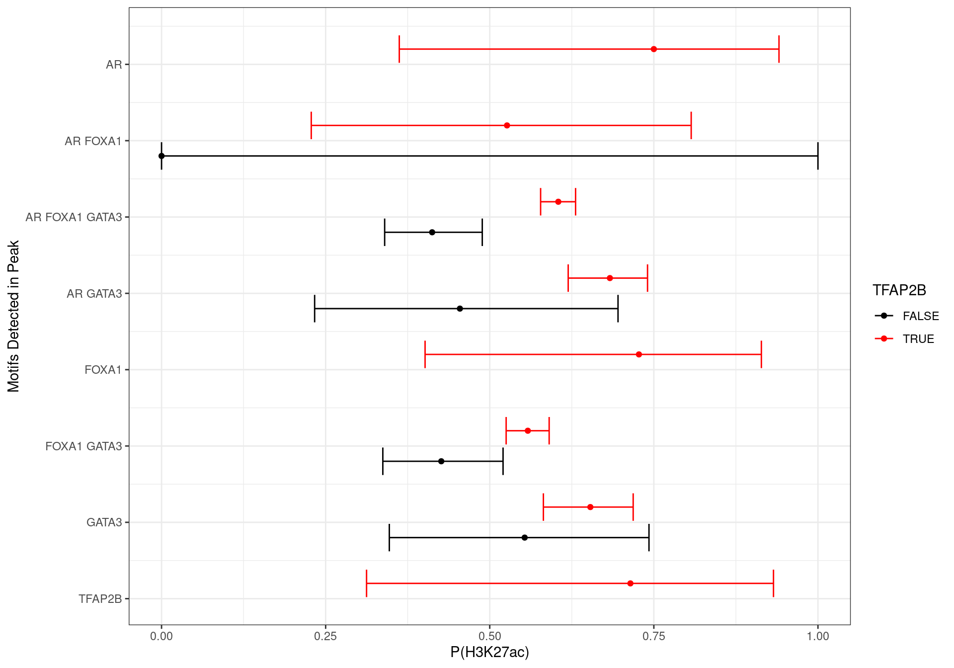
Probability of a peak being active based on the detected motifs, using H3K27ac signal as a marker of an active regulatory region. Only peaks where all four targets were detected were studied. Whilst some motif combinations suffer from low numbers, the general trend towards a strong TFAP2B motif increasing the probability of the peak being active was observed. Intervals are FWER-adjusted 95% confidence intervals, using the single-step method for estimation of the critical value.
| Version | Author | Date |
|---|---|---|
| 8dde309 | Steve Pederson | 2022-06-06 |
Motif Centrality Relative to Each Target
seq_width <- 200
min_score <- percent(0.75, accuracy = 1)
In order to assess any association in binding patterns, the binding peak (i.e.) summit of each ChIP target was taken as a viewpoint and the centrality of the best matching sequence motif for that target was assessed. Sequences were extended 200bp from each summit and the best sequence match to each binding motif were retained. Sequence matches with a score > 75% of the highest possible score were initially included before reducing matches to those with the highest score.
The motifs obtained form the larger database were all 6 motifs defined as candidate binding sites for each of the 4 ChIP targets.
meme_info %>%
  dplyr::filter(altname %in% targets) %>%
  arrange(altname, desc(icscore)) %>%
  dplyr::rename(
    `Motif ID` = name,
    Target = altname,
    IC = icscore,
    `Length (bp)` = motif_length
  ) %>%
  pander(
    justify = "llrr",
    caption = paste(
      "Motifs use for checking defined target binding sites. Motifs are ranked",
      "within each ChIP target by information content (IC)."
    )
)| Motif ID | Target | IC | Length (bp) |
|---|---|---|---|
| MA0007.2 | AR | 13.27 | 15 |
| MA0148.4 | FOXA1 | 11.41 | 12 |
| MA0037.3 | GATA3 | 9.749 | 8 |
| MA0813.1 | TFAP2B | 14.31 | 13 |
| MA0812.1 | TFAP2B | 12.56 | 11 |
| MA0811.1 | TFAP2B | 10.86 | 12 |
AR
ar_summits <- dht_peaks$AR %>%
  resize(width = 1, fix = 'start') %>%
  shift(shift = .$peak) %>%
  resize(width = seq_width, fix = 'center') %>%
  granges() %>%
  mutate(
    AR = overlapsAny(., subset(dht_consensus, AR)),
    FOXA1 = overlapsAny(., subset(dht_consensus, FOXA1)),
    GATA3 = overlapsAny(., subset(dht_consensus, GATA3)),
    TFAP2B = overlapsAny(., subset(dht_consensus, TFAP2B)),
    H3K27ac = overlapsAny(., features)
  )
seq_ar_summits <- ar_summits %>%
  get_sequence(hg19)
views_ar_summits <- as(seq_ar_summits, "Views") %>%
  setNames(names(seq_ar_summits))
matches_ar_summits <-meme_db_detected %>%
  dplyr::filter(altname %in% targets) %>%
  to_list() %>%
  lapply(
    getBestMatch,
    subject = views_ar_summits,
    min.score = min_score
  ) %>%
  setNames(
    dplyr::filter(meme_db_detected, altname %in% targets)$name
  ) %>%
  bind_rows(.id = "name") %>%
  left_join(
    dplyr::select(meme_info, name, altname, motif_length),
    by = "name"
  ) %>%
  dplyr::rename(range = view_name) %>%
  left_join(as_tibble(ar_summits), by = "range" ) %>%
  arrange(view) %>%
  mutate(
    target_detected = case_when(
      altname == "AR" ~ AR,
      altname == "FOXA1" ~ FOXA1,
      altname == "GATA3" ~ GATA3,
      altname == "TFAP2B" ~ TFAP2B
    )
  ) %>%
  dplyr::select(
    range,
    any_of(targets), H3K27ac,
    name, altname, target_detected,
    pos = start_in_view, width, strand, seq
  )
matches_ar_summits %>%
mutate(
label = glue("{name}\n({altname})"),
H3K27ac = ifelse(H3K27ac, "H3K27ac", "No H3K27ac")
) %>%
ggplot(aes(pos, stat(density), colour = altname)) +
geom_density(aes(linetype = target_detected)) +
geom_text(
aes(x = seq_width/2, y = 0.001, label = lab),
data = . %>%
group_by(label, H3K27ac) %>%
summarise(
n = dplyr::n(), .groups = "drop"
) %>%
mutate(
lab = case_when(
H3K27ac == "H3K27ac" ~ glue(
"n = {comma(n)}\n({percent(n/sum(ar_summits$H3K27ac), 0.1)})"
),
H3K27ac == "No H3K27ac" ~ glue(
"n = {comma(n)}\n({percent(n/sum(!ar_summits$H3K27ac), 0.1)})"
)
)
),
colour = "black",
inherit.aes = FALSE
) +
facet_grid(H3K27ac ~ label) +
scale_linetype_manual(values = c(3, 1)) +
labs(
x = "Best Match Position In Sequence",
y = "Density",
colour = "Motif Target",
linetype = "Target Detected"
)
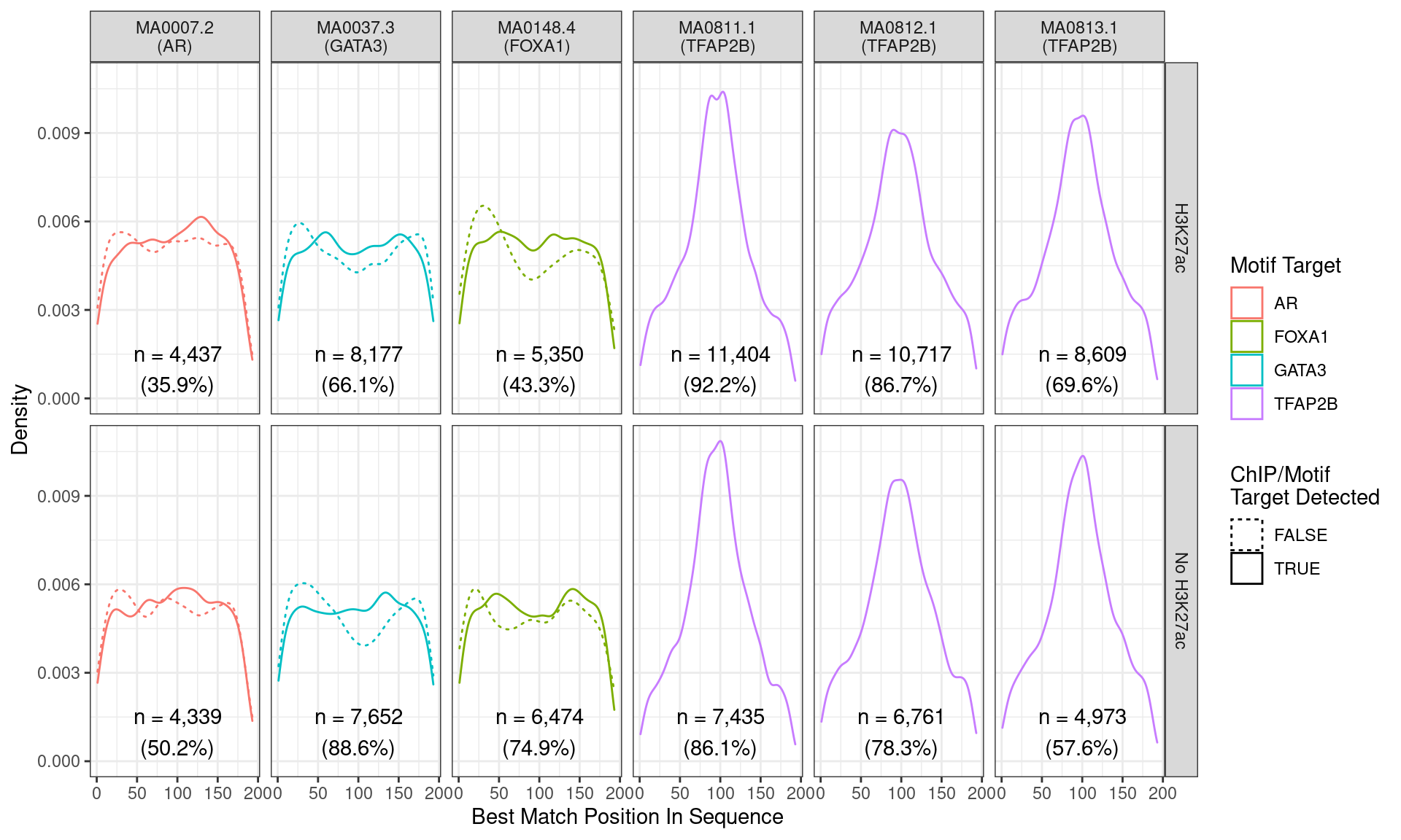
Position of the best match for each motif using sequences centred at the summits of AR binding sites. Sites where the ChIP target was not detected are shown as dashed lines, and panels are separated by H3K27ac status. No visual difference in AR motif centrality was detected due to H3K27ac signal. A slight tendency for the best FOXA1 to also appear centrally was noted.
Across all motifs which were considered to represent possible matches to the binding site of AR, matches to one or more of the motifs were found in 13,433 (69.2%) of the 19,406 queried sequences.
FOXA1
foxa1_summits <- dht_peaks$FOXA1 %>%
  resize(width = 1, fix = 'start') %>%
  shift(shift = .$peak) %>%
  resize(width = seq_width, fix = 'center') %>%
  granges() %>%
  mutate(
    AR = overlapsAny(., subset(dht_consensus, AR)),
    FOXA1 = overlapsAny(., subset(dht_consensus, FOXA1)),
    GATA3 = overlapsAny(., subset(dht_consensus, GATA3)),
    TFAP2B = overlapsAny(., subset(dht_consensus, TFAP2B)),
    H3K27ac = overlapsAny(., features)
  )
seq_foxa1_summits <- foxa1_summits %>%
  get_sequence(hg19)
views_foxa1_summits <- as(seq_foxa1_summits, "Views") %>%
  setNames(names(seq_foxa1_summits))
matches_foxa1_summits <- meme_db_detected %>%
  dplyr::filter(altname %in% targets) %>%
  to_list() %>%
  lapply(
    getBestMatch,
    subject = views_foxa1_summits,
    min.score = min_score
  ) %>%
  setNames(
    dplyr::filter(meme_db_detected, altname %in% targets)$name
  ) %>%
  bind_rows(.id = "name") %>%
  left_join(
    dplyr::select(meme_info, name, altname, motif_length),
    by = "name"
  ) %>%
  dplyr::rename(range = view_name) %>%
  left_join(as_tibble(foxa1_summits), by = "range" ) %>%
  arrange(view) %>%
  mutate(
    target_detected = case_when(
      altname == "AR" ~ AR,
      altname == "FOXA1" ~ FOXA1,
      altname == "GATA3" ~ GATA3,
      altname == "TFAP2B" ~ TFAP2B
    )
  ) %>%
  dplyr::select(
    range,
    any_of(targets), H3K27ac,
    name, altname, target_detected,
    pos = start_in_view, width, strand, seq
  )
matches_foxa1_summits %>%
mutate(
label = glue("{name}\n({altname})"),
H3K27ac = ifelse(H3K27ac, "H3K27ac", "No H3K27ac")
) %>%
ggplot(aes(pos, stat(density), colour = altname)) +
geom_density(aes(linetype = target_detected)) +
geom_text(
aes(x = seq_width/2, y = 0.001, label = lab),
data = . %>%
group_by(label, H3K27ac) %>%
summarise(
n = dplyr::n(), .groups = "drop"
) %>%
mutate(
lab = case_when(
H3K27ac == "H3K27ac" ~ glue(
"n = {comma(n)}\n({percent(n/sum(foxa1_summits$H3K27ac), 0.1)})"
),
H3K27ac == "No H3K27ac" ~ glue(
"n = {comma(n)}\n({percent(n/sum(!foxa1_summits$H3K27ac), 0.1)})"
)
)
),
colour = "black",
inherit.aes = FALSE
) +
facet_grid(H3K27ac ~ label) +
scale_linetype_manual(values = c(3, 1)) +
labs(
x = "Best Match Position In Sequence",
y = "Density",
colour = "Motif Target",
linetype = "ChIP/Motif\nTarget Detected"
)
Position of the best match for each motif using sequences centred at the summits of FOXA1 binding sites. Sites where the ChIP target was not detected are shown as dashed lines, and panels are separated by H3K27ac status. No visual difference in FOXA1 motif centrality was detected due to H3K27ac signal. A slight tendency for the best FOXA1 to also appear centrally was noted.
Across all motifs which were considered to represent possible matches to the binding site of FOXA1, matches to one or more of the motifs were found in 87,961 (94.8%) of the 92,751 queried sequences.
GATA3
gata3_summits <- dht_peaks$GATA3 %>%
  resize(width = 1, fix = 'start') %>%
  shift(shift = .$peak) %>%
  resize(width = seq_width, fix = 'center') %>%
  granges() %>%
  mutate(
    AR = overlapsAny(., subset(dht_consensus, AR)),
    FOXA1 = overlapsAny(., subset(dht_consensus, FOXA1)),
    GATA3 = overlapsAny(., subset(dht_consensus, GATA3)),
    TFAP2B = overlapsAny(., subset(dht_consensus, TFAP2B)),
    H3K27ac = overlapsAny(., features)
  )
seq_gata3_summits <- gata3_summits %>%
  get_sequence(hg19)
views_gata3_summits <- as(seq_gata3_summits, "Views") %>%
  setNames(names(seq_gata3_summits))
matches_gata3_summits <- meme_db_detected %>%
  dplyr::filter(altname %in% targets) %>%
  to_list() %>%
  lapply(
    getBestMatch,
    subject = views_gata3_summits,
    min.score = min_score
  ) %>%
  setNames(
    dplyr::filter(meme_db_detected, altname %in% targets)$name
  ) %>%
  bind_rows(.id = "name") %>%
  left_join(
    dplyr::select(meme_info, name, altname, motif_length),
    by = "name"
  ) %>%
    dplyr::rename(range = view_name) %>%
  left_join(as_tibble(gata3_summits), by = "range" ) %>%
  arrange(view) %>%
  mutate(
    target_detected = case_when(
      altname == "AR" ~ AR,
      altname == "FOXA1" ~ FOXA1,
      altname == "GATA3" ~ GATA3,
      altname == "TFAP2B" ~ TFAP2B
    )
  ) %>%
  dplyr::select(
    range,
    any_of(targets), H3K27ac,
    name, altname, target_detected,
    pos = start_in_view, width, strand, seq
  )
matches_gata3_summits %>%
mutate(
label = glue("{name}\n({altname})"),
H3K27ac = ifelse(H3K27ac, "H3K27ac", "No H3K27ac")
) %>%
ggplot(aes(pos, stat(density), colour = altname)) +
geom_density(aes(linetype = target_detected)) +
geom_text(
aes(x = seq_width/2, y = 0.001, label = lab),
data = . %>%
group_by(label, H3K27ac) %>%
summarise(
n = dplyr::n(), .groups = "drop"
) %>%
mutate(
lab = case_when(
H3K27ac == "H3K27ac" ~ glue(
"n = {comma(n)}\n({percent(n/sum(gata3_summits$H3K27ac), 0.1)})"
),
H3K27ac == "No H3K27ac" ~ glue(
"n = {comma(n)}\n({percent(n/sum(!gata3_summits$H3K27ac), 0.1)})"
)
)
),
colour = "black",
inherit.aes = FALSE
) +
facet_grid(H3K27ac ~ label) +
scale_linetype_manual(values = c(3, 1)) +
labs(
x = "Best Match Position In Sequence",
y = "Density",
colour = "Motif Target",
linetype = "ChIP/Motif\nTarget Detected"
)
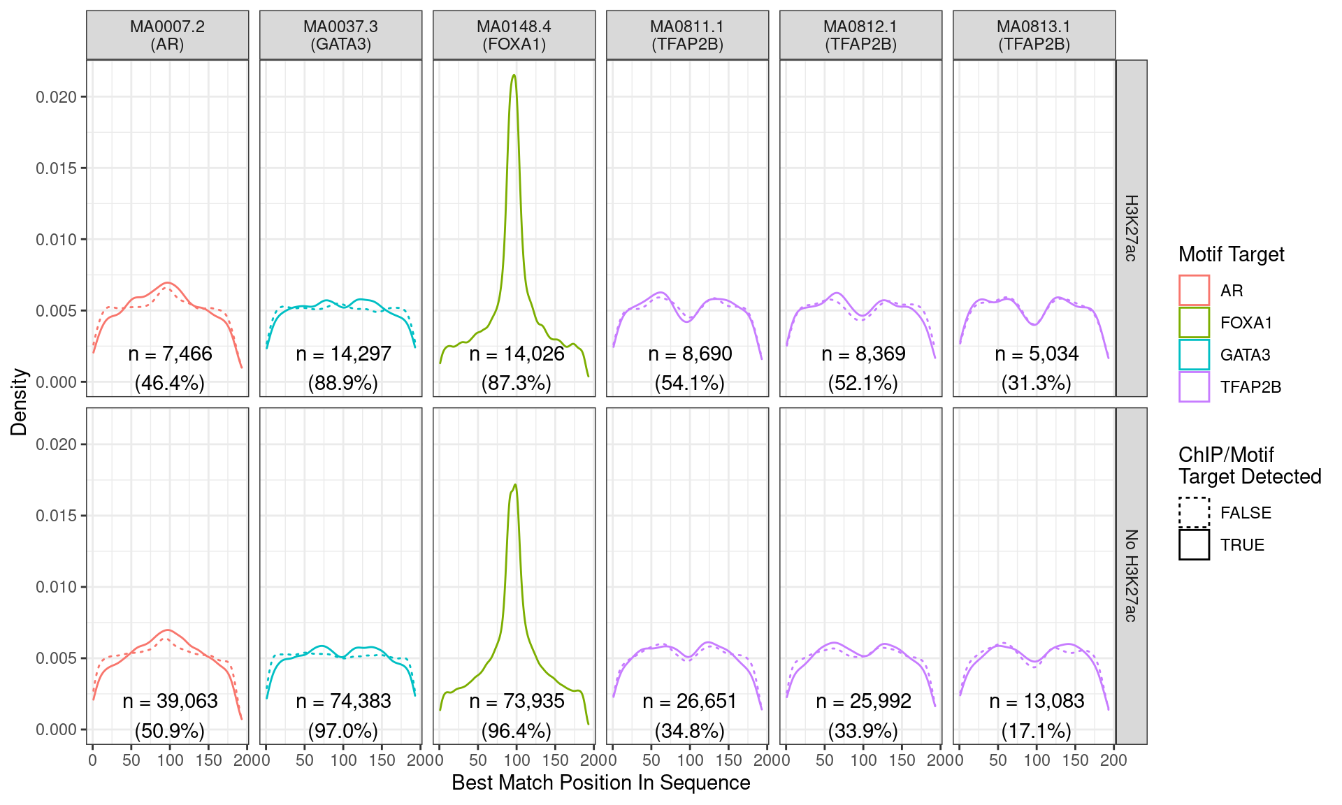
Position of the best match for each motif using sequences centred at the summits of GATA3 binding sites. Sites where the ChIP target was not detected are shown as dashed lines, and panels are separated by H3K27ac status. No visual difference in GATA3 motif centrality was detected due to H3K27ac signal. A slight tendency for the best FOXA1 to also appear centrally was noted.
Across all motifs which were considered to represent possible matches to the binding site of GATA3, matches to one or more of the motifs were found in 29,442 (99.2%) of the 29,666 queried sequences.
TFAP2B
tfap2b_summits <- dht_peaks$TFAP2B %>%
  resize(width = 1, fix = 'start') %>%
  shift(shift = .$peak) %>%
  resize(width = seq_width, fix = 'center') %>%
  granges() %>%
  mutate(
    AR = overlapsAny(., subset(dht_consensus, AR)),
    FOXA1 = overlapsAny(., subset(dht_consensus, FOXA1)),
    GATA3 = overlapsAny(., subset(dht_consensus, GATA3)),
    TFAP2B = overlapsAny(., subset(dht_consensus, TFAP2B)),
    H3K27ac = overlapsAny(., features)
  )
seq_tfap2b_summits <- tfap2b_summits %>%
  get_sequence(hg19)
views_tfap2b_summits <- as(seq_tfap2b_summits, "Views") %>%
  setNames(names(seq_tfap2b_summits))
matches_tfap2b_summits <- meme_db_detected %>%
  dplyr::filter(altname %in% targets) %>%
  to_list() %>%
  lapply(
    getBestMatch,
    subject = views_tfap2b_summits,
    min.score = min_score
  ) %>%
  setNames(
    dplyr::filter(meme_db_detected, altname %in% targets)$name
  ) %>%
  bind_rows(.id = "name") %>%
  left_join(
    dplyr::select(meme_info, name, altname, motif_length),
    by = "name"
  ) %>%
    dplyr::rename(range = view_name) %>%
  left_join(as_tibble(tfap2b_summits), by = "range" ) %>%
  arrange(view) %>%
  mutate(
    target_detected = case_when(
      altname == "AR" ~ AR,
      altname == "FOXA1" ~ FOXA1,
      altname == "GATA3" ~ GATA3,
      altname == "TFAP2B" ~ TFAP2B
    )
  ) %>%
  dplyr::select(
    range,
    any_of(targets), H3K27ac,
    name, altname, target_detected,
    pos = start_in_view, width, strand, seq
  )
matches_tfap2b_summits %>%
mutate(
label = glue("{name}\n({altname})"),
H3K27ac = ifelse(H3K27ac, "H3K27ac", "No H3K27ac")
) %>%
ggplot(aes(pos, stat(density), colour = altname)) +
geom_density(aes(linetype = target_detected)) +
geom_text(
aes(x = seq_width/2, y = 0.001, label = lab),
data = . %>%
group_by(label, H3K27ac) %>%
summarise(
n = dplyr::n(), .groups = "drop"
) %>%
mutate(
lab = case_when(
H3K27ac == "H3K27ac" ~ glue(
"n = {comma(n)}\n({percent(n/sum(tfap2b_summits$H3K27ac), 0.1)})"
),
H3K27ac == "No H3K27ac" ~ glue(
"n = {comma(n)}\n({percent(n/sum(!tfap2b_summits$H3K27ac), 0.1)})"
)
)
),
colour = "black",
inherit.aes = FALSE
) +
facet_grid(H3K27ac ~ label) +
scale_linetype_manual(values = c(3, 1)) +
labs(
x = "Best Match Position In Sequence",
y = "Density",
colour = "Motif Target",
linetype = "ChIP/Motif\nTarget Detected"
)
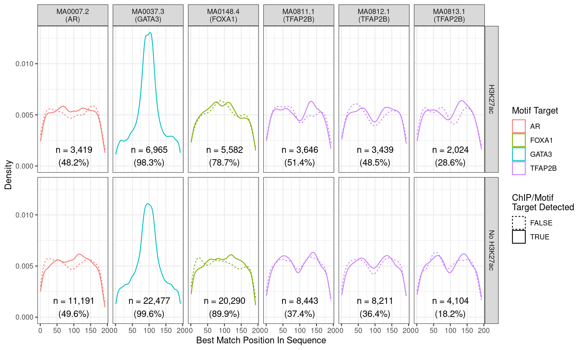
Position of the best match for each motif using sequences centred at the summits of TFAP2B binding sites. Sites where the ChIP target was not detected are shown as dashed lines, and panels are separated by H3K27ac status. No visual difference in TFAP2B motif centrality was detected. All other motifs appeared to be uniformly distributed amongst the sequences.
Across all motifs which were considered to represent possible matches to the binding site of TFAP2\(\beta\), matches to one or more of the motifs were found in 20,375 (97.0%) of the 21,008 queried sequences.
Distance Between Motifs
Whilst the above section revealed some degree of association between AR and FOXA1 sites, as well as clear separation between all targets and TFAP2B motifs, the distribution of distances between motif matches can also be addressed directly.
AR
matches_ar_summits %>%
  group_by(range) %>%
  dplyr::filter(any(altname == "AR")) %>%
  mutate(
    ar_pos = pos[altname == "AR"],
    ar_strand = strand[altname == "AR"]
  ) %>%
  ungroup() %>%
  mutate(
    ar_motif_dist = abs(pos - ar_pos),
    label = glue("{name} ({altname})"),
    H3K27ac = ifelse(H3K27ac, "H3K27ac", "No H3K27ac"),
    target_detected = ifelse(target_detected, "Target Detected", "Target Undetected")
  ) %>%
  dplyr::filter(altname != "AR") %>%
  group_by(name, target_detected, H3K27ac) %>%
  mutate(
    q = rank(ar_motif_dist, ties = "first") / length(ar_motif_dist)
  ) %>%
  dplyr::filter(q <= 0.5) %>%
  ggplot(
    aes(ar_motif_dist, q, colour = label)
  ) +
  geom_line() +
  facet_grid(H3K27ac ~ target_detected) +
  scale_y_continuous(labels= percent) +
  labs(
    x = "Distance from AR motif",
    y = "Percentile",
    colour = "Motif Target",
    linetype = "ChIP/Motif\nTarget Detected"
  )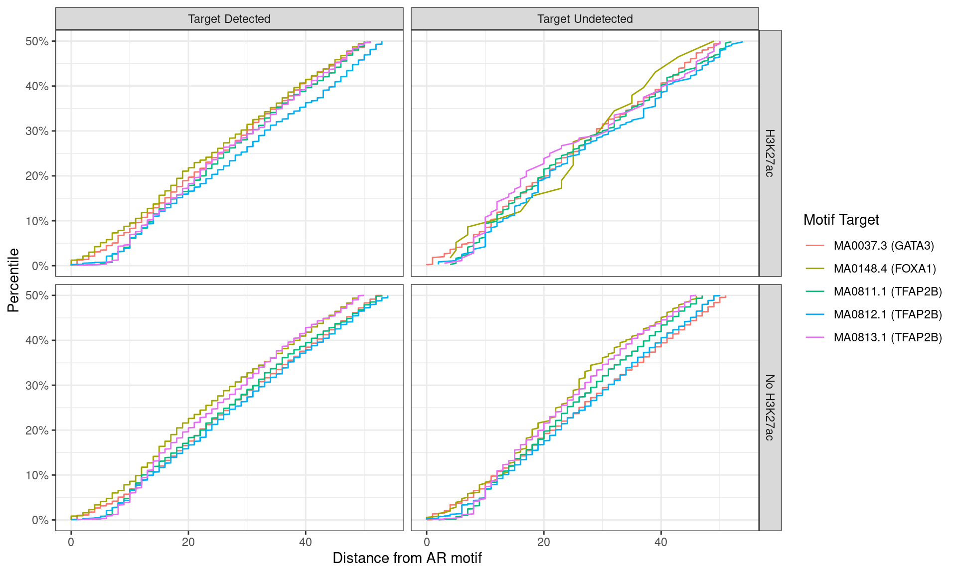
Distance between best matching motif and the best matching AR motif, showing data to the 50th percentile of distances. No noticable difference was noticed between individual motifs, H3K27ac status, or whether the ChIP target was detected within the AR peak.
FOXA1
matches_foxa1_summits %>%
  group_by(range) %>%
  dplyr::filter(any(altname == "FOXA1")) %>%
  mutate(
    foxa1_pos = pos[altname == "FOXA1"],
    foxa1_strand = strand[altname == "FOXA1"]
  ) %>%
  ungroup() %>%
  mutate(
    foxa1_motif_dist = abs(pos - foxa1_pos),
    label = glue("{name} ({altname})"),
    H3K27ac = ifelse(H3K27ac, "H3K27ac", "No H3K27ac"),
    target_detected = ifelse(target_detected, "Target Detected", "Target Undetected")
  ) %>%
  dplyr::filter(altname != "FOXA1") %>%
  group_by(name, target_detected, H3K27ac) %>%
  mutate(
    q = rank(foxa1_motif_dist, ties = "first") / length(foxa1_motif_dist)
  ) %>%
  dplyr::filter(q <= 0.5) %>%
  ggplot(
    aes(foxa1_motif_dist, q, colour = label)
  ) +
  geom_line() +
  facet_grid(H3K27ac ~ target_detected) +
  scale_y_continuous(labels= percent) +
  labs(
    x = "Distance from FOXA1 motif",
    y = "Percentile",
    colour = "Motif Target",
    linetype = "ChIP/Motif\nTarget Detected"
  )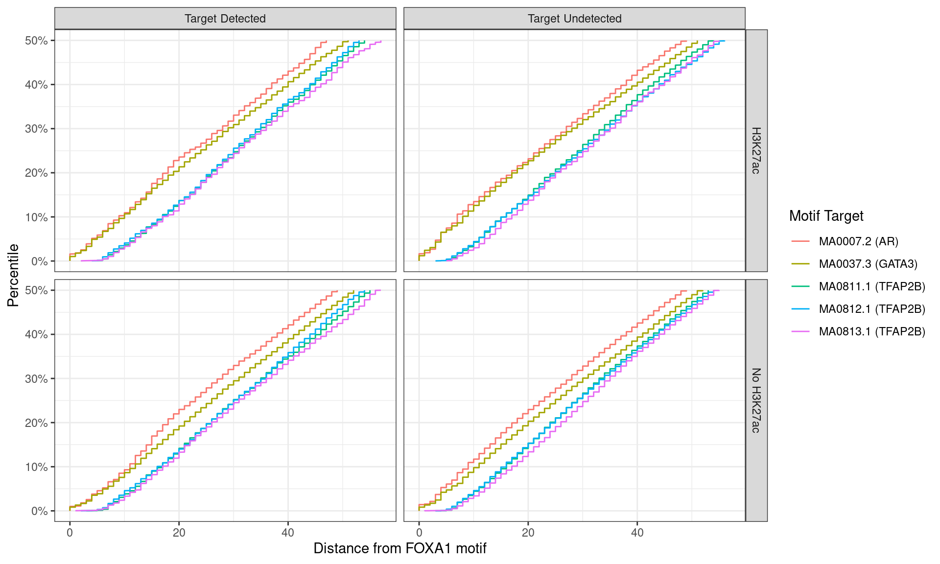
Distance between best matching motif and the best matching FOXA1 motif, showing data to the 50th percentile of distances. No noticable difference was noticed between individual motifs, H3K27ac status, or whether the ChIP target was detected within the FOXA1 peak.
GATA3
matches_gata3_summits %>%
  group_by(range) %>%
  dplyr::filter(any(altname == "GATA3")) %>%
  mutate(
    gata3_pos = pos[altname == "GATA3"],
    gata3_strand = strand[altname == "GATA3"]
  ) %>%
  ungroup() %>%
  mutate(
    gata3_motif_dist = abs(pos - gata3_pos),
    label = glue("{name} ({altname})"),
    H3K27ac = ifelse(H3K27ac, "H3K27ac", "No H3K27ac"),
    target_detected = ifelse(target_detected, "Target Detected", "Target Undetected")
  ) %>%
  dplyr::filter(altname != "GATA3") %>%
  group_by(name, target_detected, H3K27ac) %>%
  mutate(
    q = rank(gata3_motif_dist, ties = "first") / length(gata3_motif_dist)
  ) %>%
  dplyr::filter(q <= 0.5) %>%
  ggplot(
    aes(gata3_motif_dist, q, colour = label)
  ) +
  geom_line() +
  facet_grid(H3K27ac ~ target_detected) +
  scale_y_continuous(labels= percent) +
  scale_linetype_manual(values = c(3, 1)) +
  labs(
    x = "Distance from GATA3 motif",
    y = "Percentile",
    colour = "Motif Target",
    linetype = "ChIP/Motif\nTarget Detected"
  )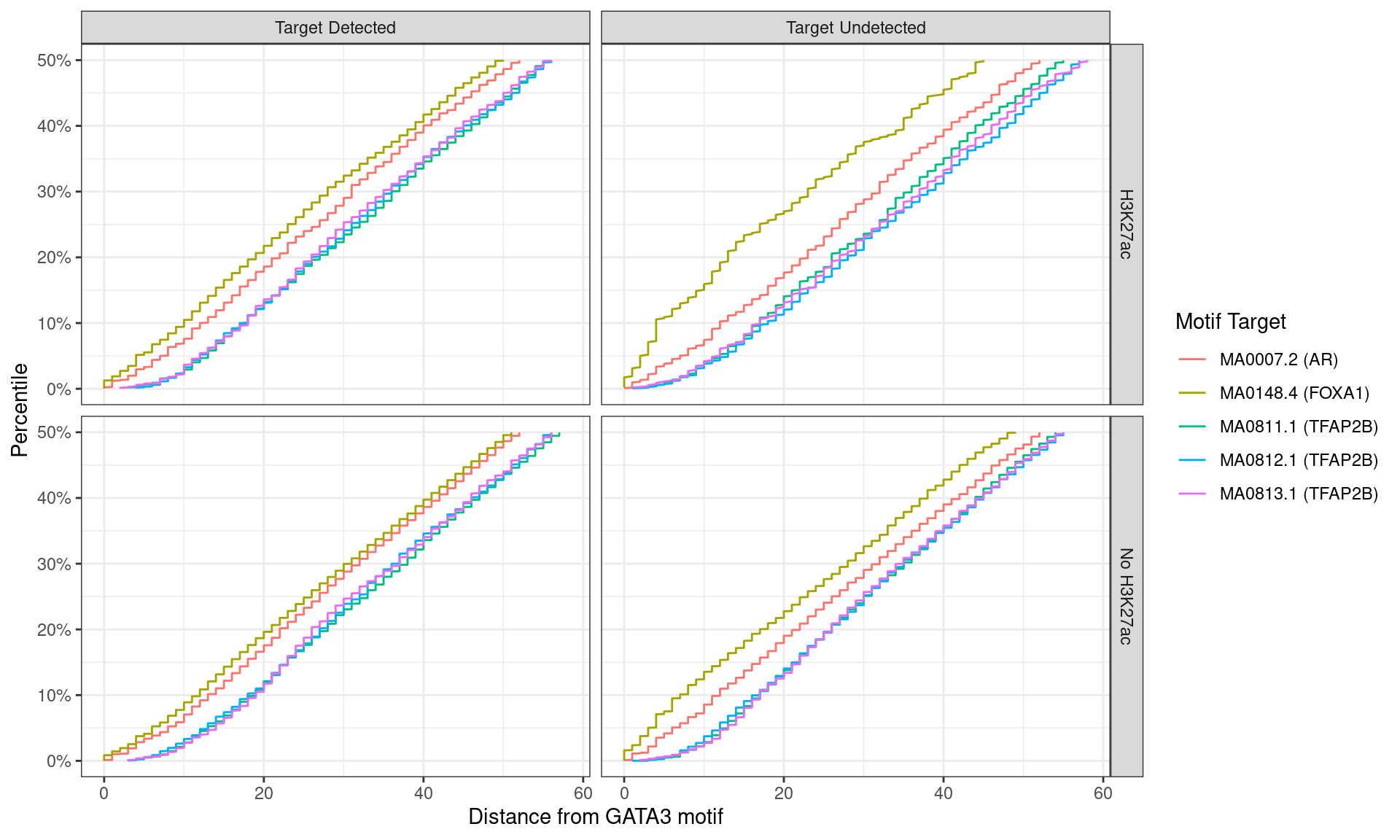
Distance between best matching motif and the best matching GATA3 motif, showing data to the 50th percentile of distances. FOXA1 motifs tended to be further from the GATA3 motif for peaks where FOXA1 was detected.
TFAP2B
matches_tfap2b_summits %>%
  group_by(range) %>%
  dplyr::filter(any(altname == "TFAP2B")) %>%
  mutate(
    tfap2b_pos = pos[altname == "TFAP2B"][1],
  ) %>%
  ungroup() %>%
  mutate(
    tfap2b_motif_dist = abs(pos - tfap2b_pos),
    label = glue("{name} ({altname})"),
    H3K27ac = ifelse(H3K27ac, "H3K27ac", "No H3K27ac"),
    target_detected = ifelse(target_detected, "Target Detected", "Target Undetected")
  ) %>%
  dplyr::filter(altname != "TFAP2B") %>%
  group_by(name, target_detected, H3K27ac) %>%
  mutate(
    q = rank(tfap2b_motif_dist, ties = "first") / length(tfap2b_motif_dist)
  ) %>%
  dplyr::filter(q <= 0.5) %>%
  ggplot(
    aes(tfap2b_motif_dist, q, colour = label)
  ) +
  geom_line() +
  facet_grid(H3K27ac ~ target_detected) +
  scale_y_continuous(labels= percent) +
  scale_linetype_manual(values = c(3, 1)) +
  labs(
    x = "Distance from TFAP2B motif",
    y = "Percentile",
    colour = "Motif Target",
    linetype = "ChIP/Motif\nTarget Detected"
  )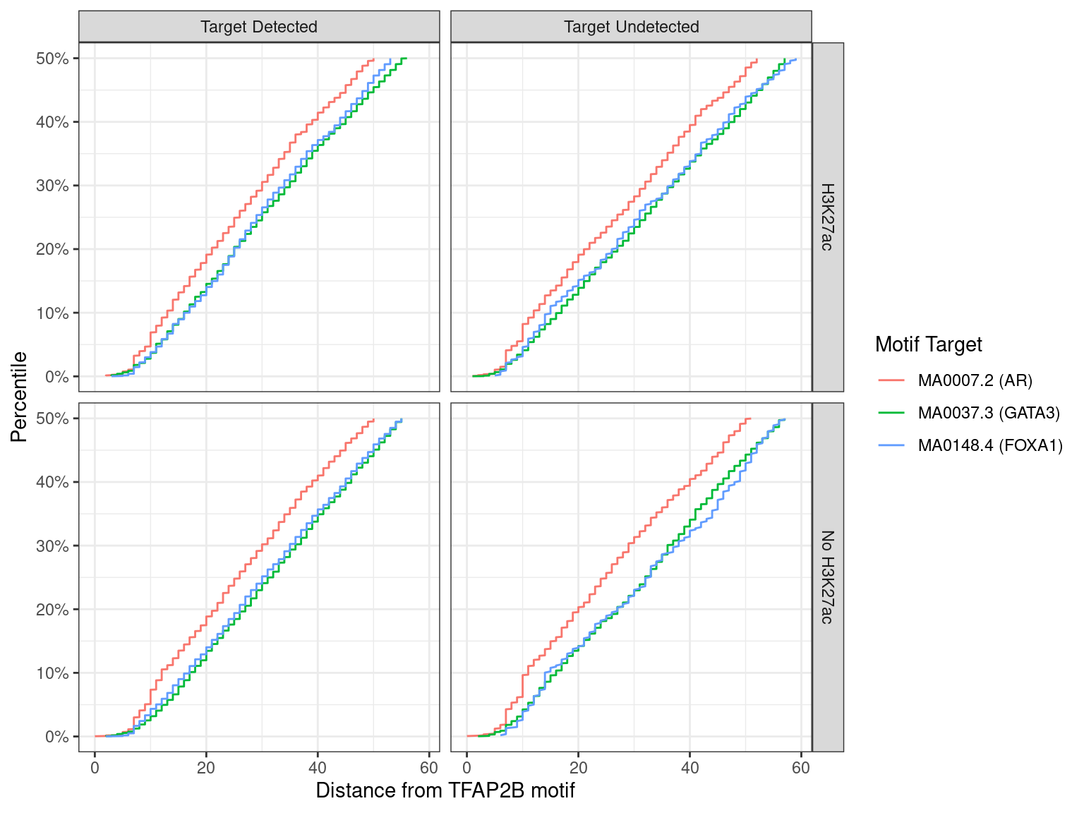
Distance between best matching motif and the best matching TFAP2B motif, showing data to the 50th percentile of distances. No noticable difference was noticed between individual motifs, H3K27ac status, or whether the ChIP target was detected within the TFAP2B peak.
sessionInfo()R version 4.2.0 (2022-04-22)
Platform: x86_64-pc-linux-gnu (64-bit)
Running under: Ubuntu 20.04.4 LTS
Matrix products: default
BLAS: /usr/lib/x86_64-linux-gnu/blas/libblas.so.3.9.0
LAPACK: /usr/lib/x86_64-linux-gnu/lapack/liblapack.so.3.9.0
locale:
[1] LC_CTYPE=en_AU.UTF-8 LC_NUMERIC=C
[3] LC_TIME=en_AU.UTF-8 LC_COLLATE=en_AU.UTF-8
[5] LC_MONETARY=en_AU.UTF-8 LC_MESSAGES=en_AU.UTF-8
[7] LC_PAPER=en_AU.UTF-8 LC_NAME=C
[9] LC_ADDRESS=C LC_TELEPHONE=C
[11] LC_MEASUREMENT=en_AU.UTF-8 LC_IDENTIFICATION=C
attached base packages:
[1] parallel stats4 stats graphics grDevices utils datasets
[8] methods base
other attached packages:
[1] multcomp_1.4-19 TH.data_1.1-1
[3] MASS_7.3-56 survival_3.2-13
[5] mvtnorm_1.1-3 htmltools_0.5.2
[7] reactable_0.3.0 UpSetR_1.4.0
[9] readxl_1.4.0 gt_0.6.0
[11] cowplot_1.1.1 glue_1.6.2
[13] pander_0.6.5 scales_1.2.0
[15] BSgenome.Hsapiens.UCSC.hg19_1.4.3 BSgenome_1.64.0
[17] Biostrings_2.64.0 XVector_0.36.0
[19] magrittr_2.0.3 rtracklayer_1.56.0
[21] extraChIPs_1.0.1 SummarizedExperiment_1.26.1
[23] Biobase_2.56.0 MatrixGenerics_1.8.0
[25] matrixStats_0.62.0 BiocParallel_1.30.2
[27] plyranges_1.16.0 GenomicRanges_1.48.0
[29] GenomeInfoDb_1.32.2 IRanges_2.30.0
[31] S4Vectors_0.34.0 BiocGenerics_0.42.0
[33] forcats_0.5.1 stringr_1.4.0
[35] dplyr_1.0.9 purrr_0.3.4
[37] readr_2.1.2 tidyr_1.2.0
[39] tibble_3.1.7 ggplot2_3.3.6
[41] tidyverse_1.3.1 universalmotif_1.14.1
[43] memes_1.4.1 workflowr_1.7.0
loaded via a namespace (and not attached):
[1] rappdirs_0.3.3 R.methodsS3_1.8.1
[3] csaw_1.30.1 bit64_4.0.5
[5] knitr_1.39 R.utils_2.11.0
[7] DelayedArray_0.22.0 data.table_1.14.2
[9] rpart_4.1.16 KEGGREST_1.36.0
[11] RCurl_1.98-1.6 AnnotationFilter_1.20.0
[13] doParallel_1.0.17 generics_0.1.2
[15] GenomicFeatures_1.48.3 callr_3.7.0
[17] EnrichedHeatmap_1.26.0 usethis_2.1.6
[19] RSQLite_2.2.14 bit_4.0.4
[21] tzdb_0.3.0 xml2_1.3.3
[23] lubridate_1.8.0 httpuv_1.6.5
[25] assertthat_0.2.1 xfun_0.31
[27] hms_1.1.1 jquerylib_0.1.4
[29] evaluate_0.15 promises_1.2.0.1
[31] fansi_1.0.3 restfulr_0.0.13
[33] progress_1.2.2 dbplyr_2.1.1
[35] igraph_1.3.1 DBI_1.1.2
[37] htmlwidgets_1.5.4 ellipsis_0.3.2
[39] crosstalk_1.2.0 backports_1.4.1
[41] biomaRt_2.52.0 vctrs_0.4.1
[43] here_1.0.1 ensembldb_2.20.1
[45] cachem_1.0.6 withr_2.5.0
[47] ggforce_0.3.3 Gviz_1.40.1
[49] vroom_1.5.7 checkmate_2.1.0
[51] GenomicAlignments_1.32.0 prettyunits_1.1.1
[53] cluster_2.1.3 lazyeval_0.2.2
[55] crayon_1.5.1 labeling_0.4.2
[57] edgeR_3.38.1 pkgconfig_2.0.3
[59] tweenr_1.0.2 pkgload_1.2.4
[61] ProtGenerics_1.28.0 nnet_7.3-17
[63] rlang_1.0.2 lifecycle_1.0.1
[65] sandwich_3.0-1 filelock_1.0.2
[67] BiocFileCache_2.4.0 modelr_0.1.8
[69] dichromat_2.0-0.1 cellranger_1.1.0
[71] rprojroot_2.0.3 polyclip_1.10-0
[73] reactR_0.4.4 Matrix_1.4-1
[75] ggseqlogo_0.1 zoo_1.8-10
[77] reprex_2.0.1 base64enc_0.1-3
[79] whisker_0.4 GlobalOptions_0.1.2
[81] processx_3.5.3 viridisLite_0.4.0
[83] png_0.1-7 rjson_0.2.21
[85] GenomicInteractions_1.30.0 bitops_1.0-7
[87] R.oo_1.24.0 cmdfun_1.0.2
[89] getPass_0.2-2 blob_1.2.3
[91] shape_1.4.6 jpeg_0.1-9
[93] memoise_2.0.1 plyr_1.8.7
[95] zlibbioc_1.42.0 compiler_4.2.0
[97] scatterpie_0.1.7 BiocIO_1.6.0
[99] RColorBrewer_1.1-3 clue_0.3-61
[101] Rsamtools_2.12.0 cli_3.3.0
[103] ps_1.7.0 htmlTable_2.4.0
[105] Formula_1.2-4 ggside_0.2.0.9990
[107] tidyselect_1.1.2 stringi_1.7.6
[109] highr_0.9 yaml_2.3.5
[111] locfit_1.5-9.5 latticeExtra_0.6-29
[113] ggrepel_0.9.1 grid_4.2.0
[115] sass_0.4.1 VariantAnnotation_1.42.1
[117] tools_4.2.0 circlize_0.4.15
[119] rstudioapi_0.13 foreach_1.5.2
[121] foreign_0.8-82 git2r_0.30.1
[123] metapod_1.4.0 gridExtra_2.3
[125] farver_2.1.0 digest_0.6.29
[127] Rcpp_1.0.8.3 broom_0.8.0
[129] later_1.3.0 httr_1.4.3
[131] AnnotationDbi_1.58.0 biovizBase_1.44.0
[133] ComplexHeatmap_2.12.0 colorspace_2.0-3
[135] rvest_1.0.2 brio_1.1.3
[137] XML_3.99-0.9 fs_1.5.2
[139] splines_4.2.0 jsonlite_1.8.0
[141] ggfun_0.0.6 testthat_3.1.4
[143] R6_2.5.1 Hmisc_4.7-0
[145] pillar_1.7.0 fastmap_1.1.0
[147] codetools_0.2-18 utf8_1.2.2
[149] lattice_0.20-45 bslib_0.3.1
[151] curl_4.3.2 limma_3.52.1
[153] rmarkdown_2.14 InteractionSet_1.24.0
[155] desc_1.4.1 munsell_0.5.0
[157] GetoptLong_1.0.5 GenomeInfoDbData_1.2.8
[159] iterators_1.0.14 haven_2.5.0
[161] gtable_0.3.0