Orthology inference: How are genes related across Schistocerca species?

workflowr

• Summary
• Checks
• Past versions

Last updated: 2025-02-10

Checks: 5 2

Knit directory: locust-comparative-genomics/

This reproducible R Markdown analysis was created with workflowr (version 1.7.1). The Checks tab describes the reproducibility checks that were applied when the results were created. The Past versions tab lists the development history.

---

R Markdown file: uncommitted changes

The R Markdown file has unstaged changes. To know which version of the R Markdown file created these results, you’ll want to first commit it to the Git repo. If you’re still working on the analysis, you can ignore this warning. When you’re finished, you can run wflow_publish to commit the R Markdown file and build the HTML.

Environment: empty

Great job! The global environment was empty. Objects defined in the global environment can affect the analysis in your R Markdown file in unknown ways. For reproduciblity it’s best to always run the code in an empty environment.

Seed: set.seed(20221025)

The command set.seed(20221025) was run prior to running the code in the R Markdown file. Setting a seed ensures that any results that rely on randomness, e.g. subsampling or permutations, are reproducible.

Session information: recorded

Great job! Recording the operating system, R version, and package versions is critical for reproducibility.

Cache: none

Nice! There were no cached chunks for this analysis, so you can be confident that you successfully produced the results during this run.

File paths: absolute

Using absolute paths to the files within your workflowr project makes it difficult for you and others to run your code on a different machine. Change the absolute path(s) below to the suggested relative path(s) to make your code more reproducible.

absolute	relative
/Users/maevatecher/Documents/GitHub/locust-comparative-genomics/data/orthofinder/Schistocerca/Results_I2/	data/orthofinder/Schistocerca/Results_I2
/Users/maevatecher/Documents/GitHub/locust-comparative-genomics/data/orthofinder/Polyneoptera/Results_I2/	data/orthofinder/Polyneoptera/Results_I2

Repository version: 34c299a

Great! You are using Git for version control. Tracking code development and connecting the code version to the results is critical for reproducibility.

The results in this page were generated with repository version 34c299a. See the Past versions tab to see a history of the changes made to the R Markdown and HTML files.

Note that you need to be careful to ensure that all relevant files for the analysis have been committed to Git prior to generating the results (you can use wflow_publish or wflow_git_commit). workflowr only checks the R Markdown file, but you know if there are other scripts or data files that it depends on. Below is the status of the Git repository when the results were generated:

Ignored files:
    Ignored:    .DS_Store
    Ignored:    analysis/.DS_Store
    Ignored:    analysis/.Rhistory
    Ignored:    data/.DS_Store
    Ignored:    data/DEG-results/.DS_Store
    Ignored:    data/WGCNA_input/.DS_Store
    Ignored:    data/WGCNA_output/.DS_Store
    Ignored:    data/behavioral_data/.DS_Store
    Ignored:    data/behavioral_data/Raw_data/.DS_Store
    Ignored:    data/list/.DS_Store
    Ignored:    data/list/GO_Annotations/.DS_Store
    Ignored:    data/orthofinder/.DS_Store
    Ignored:    data/orthofinder/Polyneoptera/.DS_Store
    Ignored:    data/orthofinder/Polyneoptera/Results_I2/.DS_Store
    Ignored:    data/orthofinder/Polyneoptera/Results_I2/Orthogroups/.DS_Store
    Ignored:    data/orthofinder/Polyneoptera/Results_I5/.DS_Store
    Ignored:    data/orthofinder/Polyneoptera/Results_I5/Orthogroups/.DS_Store
    Ignored:    data/orthofinder/Schistocerca/.DS_Store
    Ignored:    data/orthofinder/Schistocerca/Results_I2/.DS_Store
    Ignored:    data/orthofinder/Schistocerca/Results_I2/Orthogroups/.DS_Store
    Ignored:    data/orthofinder/Schistocerca/Results_I5/.DS_Store
    Ignored:    data/orthofinder/Schistocerca/Results_I5/Orthogroups/.DS_Store
    Ignored:    data/overlap/.DS_Store
    Ignored:    data/readcounts/.DS_Store

Untracked files:
    Untracked:  analysis/3_compiling_tables.Rmd
    Untracked:  data/orthofinder/Polyneoptera/Results_I5/Orthogroups/Orthogroups.tsv
    Untracked:  data/orthofinder/Polyneoptera/Results_I5/Orthogroups/Orthogroups.txt
    Untracked:  data/orthofinder/Polyneoptera/Results_I5/Orthogroups/Orthogroups_reprocessed.tsv
    Untracked:  data/orthofinder/Polyneoptera/Results_I5/Orthogroups/Orthogroups_reprocessed.txt
    Untracked:  data/orthofinder/Schistocerca/Results_I2/Orthogroups/Orthogroups.tsv
    Untracked:  data/orthofinder/Schistocerca/Results_I2/Orthogroups/Orthogroups.txt
    Untracked:  data/orthofinder/Schistocerca/Results_I2/Orthogroups/Orthogroups_reprocessed.tsv
    Untracked:  data/orthofinder/Schistocerca/Results_I2/Orthogroups/Orthogroups_reprocessed.txt

Unstaged changes:
    Modified:   analysis/2_orthologs-prediction.Rmd
    Modified:   data/orthofinder/Polyneoptera/Results_I2/Orthogroups_13species_Jan2025.txt
    Modified:   data/orthofinder/Polyneoptera/Results_I2/Orthogroups_genesprotein_Schisto_Jan2025.txt
    Modified:   data/orthofinder/Polyneoptera/Results_I2/Orthogroups_genesproteinbiotype_13species_Jan2025.csv
    Modified:   data/orthofinder/Polyneoptera/Results_I2/Plots_Polyneoptera/VerticalStackedBar_A. simplex.pdf
    Modified:   data/orthofinder/Polyneoptera/Results_I2/Plots_Polyneoptera/VerticalStackedBar_B. rossius.pdf
    Modified:   data/orthofinder/Polyneoptera/Results_I2/Plots_Polyneoptera/VerticalStackedBar_C. secundus.pdf
    Modified:   data/orthofinder/Polyneoptera/Results_I2/Plots_Polyneoptera/VerticalStackedBar_D. australis.pdf
    Modified:   data/orthofinder/Polyneoptera/Results_I2/Plots_Polyneoptera/VerticalStackedBar_G. bimaculatus.pdf
    Modified:   data/orthofinder/Polyneoptera/Results_I2/Plots_Polyneoptera/VerticalStackedBar_G. longicornis.pdf
    Modified:   data/orthofinder/Polyneoptera/Results_I2/Plots_Polyneoptera/VerticalStackedBar_P. americana.pdf
    Modified:   data/orthofinder/Polyneoptera/Results_I2/Plots_Polyneoptera/VerticalStackedBar_americana.pdf
    Modified:   data/orthofinder/Polyneoptera/Results_I2/Plots_Polyneoptera/VerticalStackedBar_cancellata.pdf
    Modified:   data/orthofinder/Polyneoptera/Results_I2/Plots_Polyneoptera/VerticalStackedBar_cubense.pdf
    Modified:   data/orthofinder/Polyneoptera/Results_I2/Plots_Polyneoptera/VerticalStackedBar_gregaria.pdf
    Modified:   data/orthofinder/Polyneoptera/Results_I2/Plots_Polyneoptera/VerticalStackedBar_nitens.pdf
    Modified:   data/orthofinder/Polyneoptera/Results_I2/Plots_Polyneoptera/VerticalStackedBar_piceifrons.pdf
    Modified:   data/orthofinder/Polyneoptera/Results_I2/SingleCopyOrthogroups_genesprotein_13species_Jan2025.txt
    Modified:   data/orthofinder/Schistocerca/Results_I2/Orthogroups_Schistocerca_Jan2025.txt
    Modified:   data/orthofinder/Schistocerca/Results_I2/Orthogroups_genesproteinbiotype_Schistocerca_Jan2025.csv
    Modified:   data/orthofinder/Schistocerca/Results_I2/Plots_Schistocerca/VerticalStackedBar_americana.pdf
    Modified:   data/orthofinder/Schistocerca/Results_I2/Plots_Schistocerca/VerticalStackedBar_cancellata.pdf
    Modified:   data/orthofinder/Schistocerca/Results_I2/Plots_Schistocerca/VerticalStackedBar_cubense.pdf
    Modified:   data/orthofinder/Schistocerca/Results_I2/Plots_Schistocerca/VerticalStackedBar_gregaria.pdf
    Modified:   data/orthofinder/Schistocerca/Results_I2/Plots_Schistocerca/VerticalStackedBar_nitens.pdf
    Modified:   data/orthofinder/Schistocerca/Results_I2/Plots_Schistocerca/VerticalStackedBar_piceifrons.pdf
    Modified:   data/orthofinder/Schistocerca/Results_I2/SingleCopyOrthogroups_genesprotein_6species_Jan2025.txt
    Deleted:    data/overlap/summary_DEGs_Orthogroups_togregaria.csv

Note that any generated files, e.g. HTML, png, CSS, etc., are not included in this status report because it is ok for generated content to have uncommitted changes.

---

These are the previous versions of the repository in which changes were made to the R Markdown (analysis/2_orthologs-prediction.Rmd) and HTML (docs/2_orthologs-prediction.html) files. If you’ve configured a remote Git repository (see ?wflow_git_remote), click on the hyperlinks in the table below to view the files as they were in that past version.

File	Version	Author	Date	Message
Rmd	db8b525	Maeva TECHER	2025-02-06	update overlap
html	db8b525	Maeva TECHER	2025-02-06	update overlap
Rmd	e55bac6	Maeva TECHER	2025-01-26	Updating the github
html	e55bac6	Maeva TECHER	2025-01-26	Updating the github
Rmd	faf2db3	Maeva TECHER	2025-01-13	update markdown
html	faf2db3	Maeva TECHER	2025-01-13	update markdown
Rmd	b80db34	Maeva TECHER	2025-01-13	Adding selection analysis part
html	b80db34	Maeva TECHER	2025-01-13	Adding selection analysis part
Rmd	3fa8e62	Maeva TECHER	2024-11-09	updated analysis
html	3fa8e62	Maeva TECHER	2024-11-09	updated analysis
Rmd	edb70fe	Maeva TECHER	2024-11-08	overlap and deg results created
html	edb70fe	Maeva TECHER	2024-11-08	overlap and deg results created
html	7f1d1fe	Maeva TECHER	2024-11-01	Build site.
Rmd	f01f1cf	Maeva TECHER	2024-11-01	Adding new files and docs
html	f01f1cf	Maeva TECHER	2024-11-01	Adding new files and docs
html	ba35b82	Maeva A. TECHER	2024-06-20	Build site.
html	c006e71	Maeva A. TECHER	2024-06-20	change
html	82ef59f	Maeva A. TECHER	2024-05-16	Build site.
Rmd	151afb3	Maeva A. TECHER	2024-05-16	wflow_publish("analysis/2_orthologs-prediction.Rmd")
html	4dd0e26	Maeva A. TECHER	2024-05-15	Build site.
Rmd	38ef822	Maeva A. TECHER	2024-05-15	wflow_publish("analysis/2_orthologs-prediction.Rmd")
html	ce82fe8	Maeva A. TECHER	2024-05-14	Build site.
Rmd	3ca5aee	Maeva A. TECHER	2024-05-14	wflow_publish("analysis/2_orthologs-prediction.Rmd")
html	ac06f45	Maeva A. TECHER	2024-05-14	Build site.
Rmd	be09a11	Maeva A. TECHER	2024-05-14	update markdown
html	be09a11	Maeva A. TECHER	2024-05-14	update markdown
html	0837617	Maeva A. TECHER	2024-01-30	Build site.
html	f701a01	Maeva A. TECHER	2024-01-30	reupdate
html	2ca8696	Maeva A. TECHER	2024-01-30	Build site.
html	5c5487e	Maeva A. TECHER	2024-01-30	Build site.
html	0135a6e	Maeva A. TECHER	2024-01-30	Build site.
Rmd	505a8dc	Maeva A. TECHER	2024-01-30	wflow_publish("analysis/2_orthologs-prediction.Rmd")
html	579056a	Maeva A. TECHER	2024-01-30	Build site.
Rmd	f50a3dd	Maeva A. TECHER	2024-01-30	wflow_publish("analysis/2_orthologs-prediction.Rmd")
html	f831779	Maeva A. TECHER	2024-01-24	Build site.
html	1b09cbe	Maeva A. TECHER	2024-01-24	remove
html	79006db	Maeva A. TECHER	2024-01-24	Build site.
Rmd	b195f57	Maeva A. TECHER	2024-01-24	refresh
html	b195f57	Maeva A. TECHER	2024-01-24	refresh
html	dfc68c7	Maeva A. TECHER	2023-12-18	Build site.
Rmd	53877fa	Maeva A. TECHER	2023-12-18	add pages

---

Comparative genomics and ortholog genes with OrthoFinder

We wanted to compare the six genomes of Schistocerca to get insights on gene evolution and relationships regarding their numbers, content, function and location. In order to achieve this, we need to identify groups of orthologous genes among our species of interest, considering at least one outgroup.

Orthologs are genes from different species that originated from a single ancestral gene and evolved through speciation events. However since genes can be lost or duplicated during evolution, some genes may not have exactly one orthologue in the genome of another species. Here we will separate the 1:1 orthologs to the the concept of orthogroups. Orthogroups can contain 1:1 orthologs but also several several orthologs from different species, including paralogs and one-to-many orthologs. Paralogs are genes within the same species that have originated from a shared ancestral genes but have diverged over time following gene duplication events.

Note:We used OrthoFinder to identify the orthogroups using amino acid sequences from the longest isoform of each gene. For this part, refers to the well curated pipeline FormicidaeMolecularEvolution by Megan Barkdull (Assistant Curator of Entomology at the Natural History Museum of Los Angeles County). We describe below the modifications made and mostly copied the workflow from her Github.

1. Downloading data

We created the file “input-XXX.txt” as described to automatically download the coding sequence, protein sequence, GFF annotation data for each of our six Schistocerca species and annotated outgroups. The outgroups were choosen as close phylogenetic species with a RefSeq genome showing 1) a chromosome length, 2) associated with an annotation, 3) large size and 4) hybrid techniques used for assembly (last NCBI search: 28 April 2024).

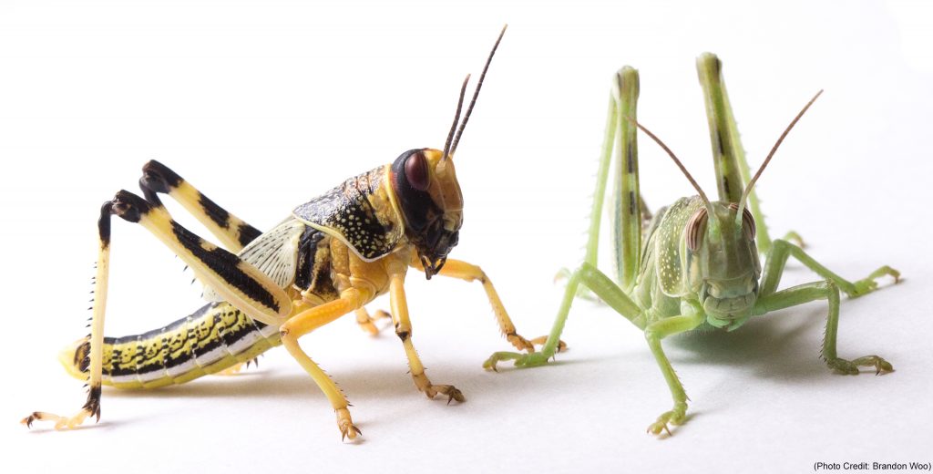
Our target species for this study:
* The desert locust Schistocerca gregaria
* The South American locust Schistocerca cancellata
* The Central American locust Schistocerca piceifrons
* The American grasshopper Schistocerca americana
* The bird grasshopper Schistocerca serialis cubense
* The vagrant locust Schistocerca nitens

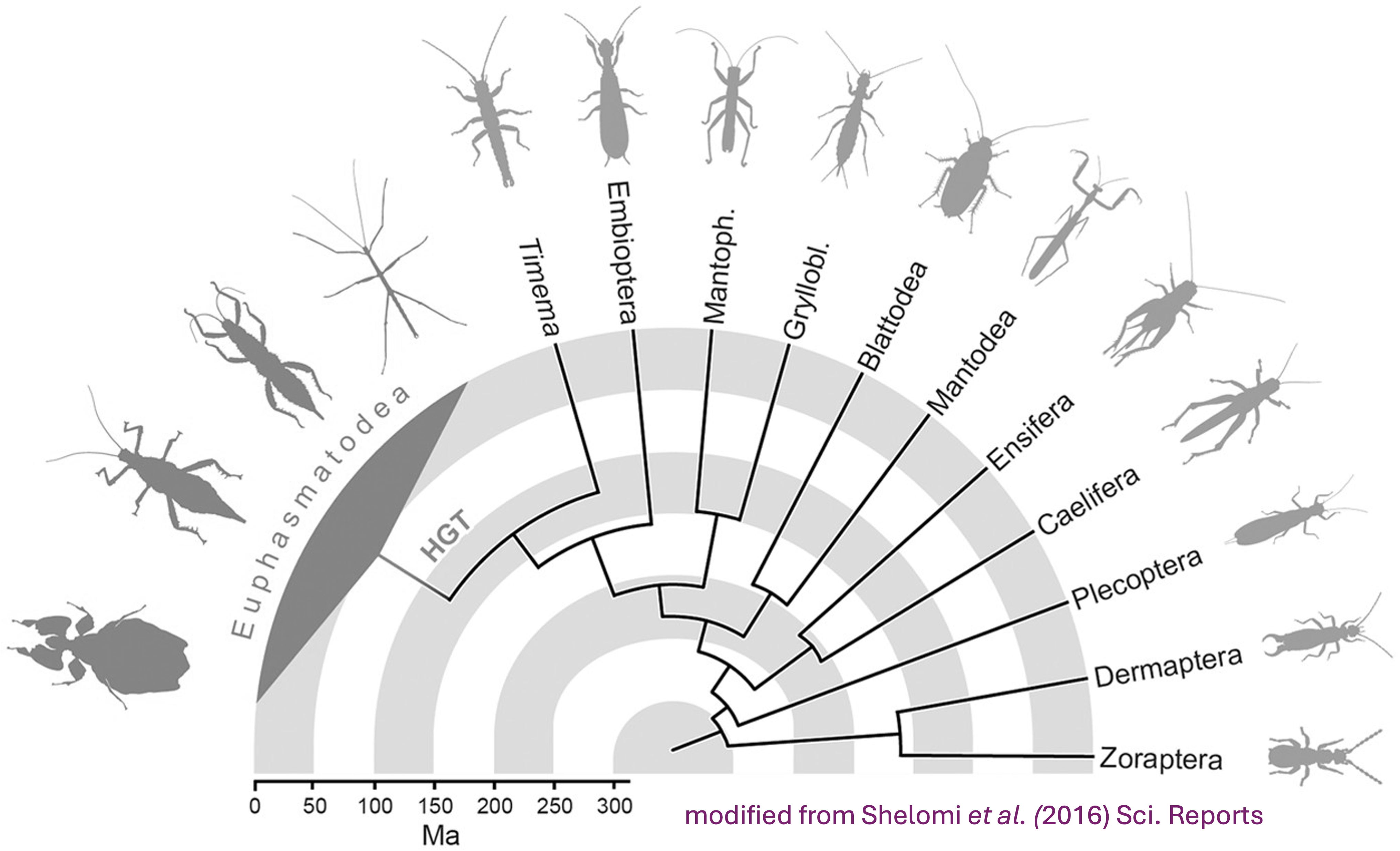
Our Polyneoptera outgroup species:
* The Mormon cricket Anabrus simplex. Reason: Orthoptera close relative available with chromosome length.
* The long cercus field cricket Gryllus longicercus. Reason: Orthoptera close relative available with scaffold length and a user submitted annotation.
* The two-spotted cricket Gryllus bimaculatus. Reason: Orthoptera close relative available with chromosome length.
* The Lord Howe Island stick insect Dryococelus australis. Reason: Polyneoptera close relative available with chromosome length.
* The European stick insect Bacillus rossius redtenbacheri. Reason: Polyneoptera close relative available with chromosome length.
* The drywood termite Cryptotermes secundus. Reason: Eusocial insect with caste determination phenotypic plasticity.
* The American cockroach Periplaneta americana. Reason: Polyneoptera close relative available with chromosome length.

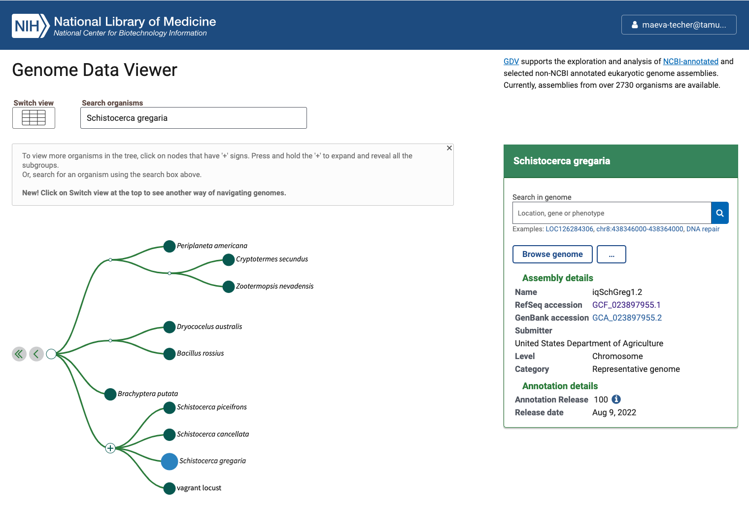
Status of Genome Data Viewer on NCBI for selecting our outgroups

NB: During our search, we identified very valuable genomes but for which no annotation was available (e.g., CAU_Lmig_1.0 for Locusta migratoria , iqMecThal1.2 Meconema thalassinum). However upon request to NCBI team, we were informed that the Locusta genome has not been annotated because of the presence of large bacterial contamination and Meconema does not possess RNA SRAs to help with the annotation.

Using the FTP NCBI link associated with each RefSeq, we created the input file.

./scripts/DataDownload ./scripts/inputurls_18polyneoptera_Nov2024.txt 

On the TAMU Grace cluster, when you download do not run it on a node as it does not work. Run it from the login node or transfer the files already preloaded. This will creates a folder ./1_RawData with 3 files for each species.

In summary, below are the details of each RefSeq annotation that we will be using as input for OrthoFinder. It will be important to check that after steps 2-4, the number of protein coding genes OrthoFinder is similar to the initial input.

	Genomic Information of the genomes used as input for OrthoFinder
Species	Order	Status	Genome_Size	Annotated_Genes	Protein_Coding
Schistocerca gregaria	Orthoptera	Locust	8.7 Gb	99467	19799
Schistocerca cancellata	Orthoptera	Locust	8.5 Gb	103533	16907
Schistocerca piceifrons	Orthoptera	Locust	8.7 Gb	96806	17490
Schistocerca americana	Orthoptera	Grasshopper	9.0 Gb	81274	17662
Schistocerca serialis cubense	Orthoptera	Grasshopper	9.1 Gb	75810	17237
Schistocerca nitens	Orthoptera	Grasshopper	8.8 Gb	72560	17500
Anabrus simplex (Idaho)	Orthoptera	Outgroup	6.4 Gb	27091	14866
Gryllus bimaculatus	Orthoptera	Outgroup	1.7 Gb	17871	NA
Gryllus longicercus	Orthoptera	Outgroup	1.9 Gb	14831	NA
Bacillus rossius redtenbacheri	Phasmatodea	Outgroup	1.6 Gb	19298	14448
Dryococelus australis	Phasmatodea	Outgroup	3.4 Gb	33793	NA
Periplaneta americana	Blattodea	Outgroup	3.1 Gb	28416	28414
Cryptotermes secundus	Blattodea	Outgroup	3.1 Gb	27047	NA

2. Selecting longest isoforms

Here again, we will follow the pipeline except that to run it on Grace cluster we will make small modifications. The idea is that we will use only the single longest isoform of each gene to ease the orthology analysis. While this might not always be the principal isoform of said gene, we will apply the same bias to all genes the same way.

To run R without bothering other users, we will claim one interactive node to make sure we can proactively update the package if there are some issues:

srun --ntasks 1 --cpus-per-task 4 --mem 10G --time 01:00:00 --pty bash

Then we will use any package preloaded on the cluster before needed to install our own on our user library if needed. We will need Pandoc for loading orthologr

ml GCC/12.2.0  OpenMPI/4.1.4 R_tamu/4.3.1
export R_LIBS=$SCRATCH/R_LIBS_USER/
ml Pandoc/2.13

We now simply run the script as indicated on the pipeline page:

./scripts/GeneRetrieval.R ./scripts/inputurls_13polyneoptera_Jan2025.txt

---

If the annotated genome is not done by RefSeq but submitted by users:
When downloading genomes from NCBI, we found a few interesting ones that were but annotated by users with a different format than NCBI Gnomon pipeline. For example on the image below (when you zoom in), we can see that the gene= field is present in RefSeq but is not in users submitted but could be created using ID= field.

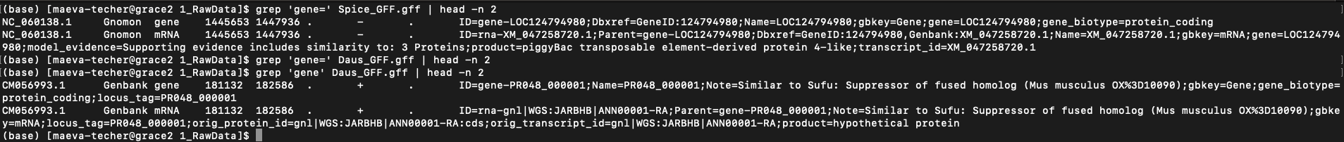
Example of difference in the presence of “gene” field between S. piceifrons and Dryococelus australis (3.4Gb).

To correct, I ran the following parsing code which append a new gene column based on locus_tag:

# we need to modify the GFF, proteins and genome/transcript fasta file
sed -i 's/locus_tag=/gene=/g' {SPECIES}_GFF.gff
sed -i 's/locus_tag=/gene=/g' {SPECIES}_proteins.faa
sed -i 's/locus_tag=/gene=/g' {SPECIES}_transcripts.fasta

# then we check 
grep 'gene=' {SPECIES}_GFF.gff | head -n 10

We did it for Daus_GFF.gff, Dpunc_GFF.gff, Gbima_GFF.gff, Glong_GFF.gff, Pamer_GFF.gff and Tpodu_GFF.gff. Then instead of running the GeneRetrieval.R, we computed manually (to check if error) using the following R script:

library(orthologr)
library(tidyverse)
library(biomartr)
library(phylotools)
library(data.table)

# Define the species parameter
species <- "Gbima" # for example
#species <- "Glong"
#species <- "Daus"
#species <- "Dpunc"
#species <- "Pamer"
#species <- "Tpodu"

# Define file paths based on the species parameter
proteomeFile <- paste0("./1_RawData/", species, "_proteins.faa")
annotationFile <- paste0("./1_RawData/", species, "_GFF.gff")
longestIsoformsFile <- paste0("./2_LongestIsoforms/", species, "_longestIsoforms.fasta")
transcriptsFile <- paste0("./1_RawData/", species, "_transcripts.fasta")
filteredTranscriptsOutput <- paste0("./2_LongestIsoforms/", species, "_filteredTranscripts.fasta")

    
# Step 1: Retrieve the longest isoforms for Glong
retrieve_longest_isoforms(
  proteome_file = proteomeFile,
  annotation_file = annotationFile,
  new_file = longestIsoformsFile,
  annotation_format = "gff"
)
    
# Step 2: Load longest isoforms and transcript files
isoforms <- phylotools::read.fasta(longestIsoformsFile)
isoform_ids <- isoforms$seq.name  # Get IDs of longest isoforms
isoform_ids
transcripts <- phylotools::read.fasta(transcriptsFile)
head(transcripts$seq.name)

# Step 3: Adjust headers in transcripts to match core identifiers
transcripts$seq.name <- str_extract(transcripts$seq.name, "(?<=cds_)[^ ]+")  # Extract main identifier
transcripts$seq.name <- str_extract(transcripts$seq.name, "^[^_]+")  # Keep only core ID without suffix
transcripts$seq.name

# Step 4: Filter transcripts to keep only those matching isoform IDs
filtered_transcripts <- transcripts %>%
  filter(seq.name %in% isoform_ids)

# Step 5: Write the filtered transcripts to a new FASTA file with simplified headers
phylotools::dat2fasta(filtered_transcripts, outfile = filteredTranscriptsOutput)

message("Filtered transcripts for ", species, " saved to: ", filteredTranscriptsOutput)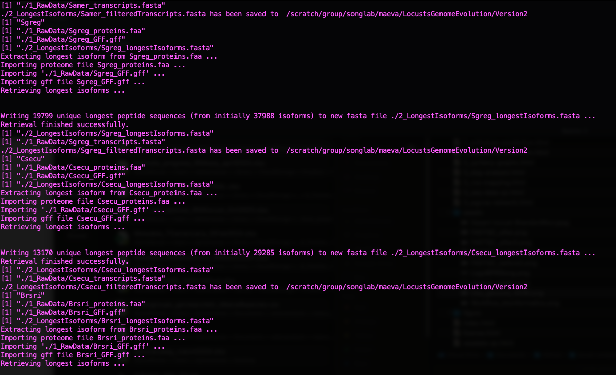

---

Status of Gene Retrieval script when successful

Longest isoforms kept for each genome following using orthologr
Species	Total_Peptides	Number_Kept_Isoforms
Schistocerca gregaria	37988	19799
Schistocerca cancellata	26362	16907
Schistocerca piceifrons	25717	17490
Schistocerca americana	26125	17662
Schistocerca serialis cubense	27654	17237
Schistocerca nitens	28445	17500
Anabrus simplex (Idaho)	X	X
Gryllus bimaculatus	25032	17871
Gryllus longicercus	19656	14730
Bacillus rossius redtenbacheri	29758	14448
Dryococelus australis	33111	33111
Periplaneta americana	27047	27047
Cryptotermes secundus	29285	13170

3. Cleaning the raw data

For the cleaning step of the mbarkdull’s pipeline we simply followed the command line with no modifications.

./scripts/DataCleaning ./scripts/inputurls_13polyneoptera_Jan2025.txt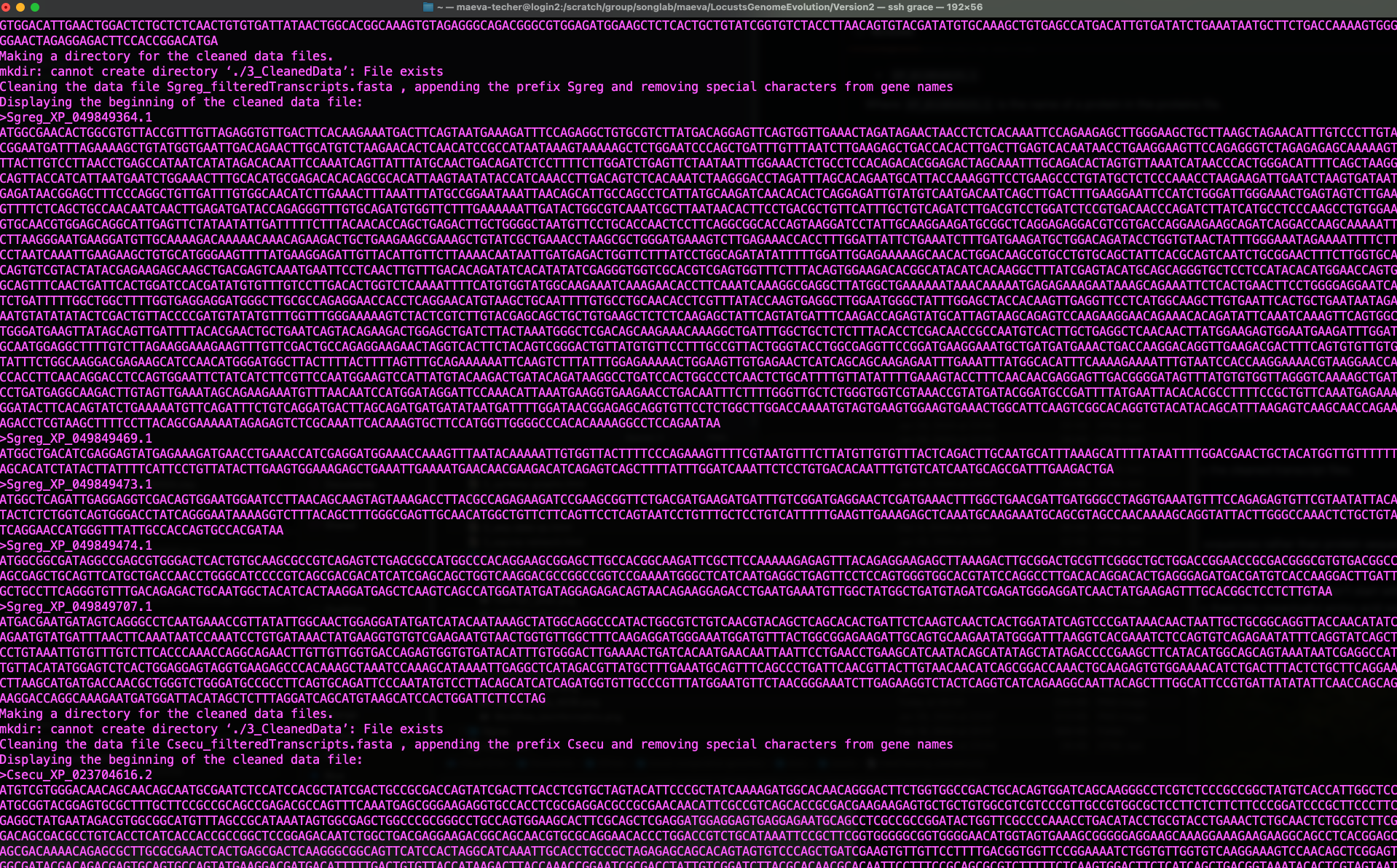 

Status of Data Cleaning script when successful

4. Translating nucleotide sequences to amino acid sequences

This step does not seems to be really necessary because Orthofinder can immediately take the XXX_longestIsoforms.fasta files. We just run the scriptDataCleaningIsoforms_modif on it to rename and clean it.:

As mentioned in the pipeline page, we will mostly need to use amino acid sequences rather than protein and we need to translate the data we downloaded. We will be using the Python script from mbarkdull ./scripts/TranscriptFilesTranslateScript.py but before that we will modify our input file to only include only the 12 essential species.

We changed the script in head lines and lines 25-27, to call the module directly from the cluster as follow:

#!/bin/bash

##NECESSARY JOB SPECIFICATIONS
#SBATCH --job-name=Transdecoder         #Set the job name to "JobExample4"
#SBATCH --time=02:00:00         #Set the wall clock limit to 1hr and 30min
#SBATCH --ntasks=2              #Request 2 task
#SBATCH --cpus-per-task=4       #Request 8 task
#SBATCH --mem=20G              #Request 50GB per node

ml GCC/10.2.0 OpenMPI/4.0.5 TransDecoder/5.5.0 Biopython/1.78

   # Now we can run Transdecoder on the cleaned file:
    echo "First, attempting TransDecoder run on $cleanName"
    ml GCC/10.2.0 OpenMPI/4.0.5 TransDecoder/5.5.0
    TransDecoder.LongOrfs -t $cleanName
    TransDecoder.Predict -t $cleanName --single_best_only

and then we launched the script by changing the top lines to put in sbatch:

sbatch ./scripts/DataTranslating_modif ./scripts/inputurls_13polyneoptera_Jan2025.txt 

5. Running Orthofinder

Now we will finally run Orthofinder to identify groups of orthologous genones in our translated amino acid sequences. We will also use MAFFT to produce multiple sequence alignment across our six species of Schistocerca and the outgroups.

Instead of using the ./scripts/DataOrthofinder from the pipeline, we will be running our own command line here. Before doing so, we did manually the creating of folders and moving of fasta files as follow:

  mkdir LocustsGenomeEvolution/tmp
  mkdir -p ./5_OrthoFinder/fasta
  cp ./4_1_TranslatedData/OutputFiles/translated* ./5_OrthoFinder/fasta
  cp ./3_CleanedData/*longestIsoforms.fasta ./5_OrthoFinder/fasta
  cd ./5_OrthoFinder/fasta
  rename translated '' translated*
  
  # Loop through files and rename them
for file in cleaned*_longestIsoforms.fasta; do
    # Remove "cleaned" and replace "_longestIsoforms" with "_filteredproteome"
    new_name=$(echo "$file" | sed 's/^cleaned//; s/_longestIsoforms/_filteredproteome/')
    mv "$file" "$new_name"
done
  cd ../

You can also rename them with a simple name like “S_americana.fasta”, this will help ease the visualization later on.

To run orthofinder onto our Grace cluster, I checked the compatibility of the modules required and these are the versions acceptable to run in sbatchorthofinder.sh:

#!/bin/bash

##NECESSARY JOB SPECIFICATIONS
#SBATCH --job-name=orthofinder-blast        #Set the job name to "JobExample4"
#SBATCH --time=2-00:00:00         #Set the wall clock limit to 1hr and 30min
#SBATCH --ntasks=1              #Request 1 task
#SBATCH --cpus-per-task=48       #Request 1 task
#SBATCH --mem=50G              #Request 100GB per node


module purge 
ml iccifort/2019.5.281  impi/2018.5.288 OrthoFinder/2.3.11-Python-3.7.4 
ml IQ-TREE/1.6.12 FastTree/2.1.11
ml MAFFT/7.453-with-extensions

proteome_dir="/scratch/group/songlab/maeva/LocustsGenomeEvolution/Version3/5_OrthoFinder/fasta"
temporary_dir="/scratch/group/songlab/maeva/LocustsGenomeEvolution/tmp"

# Check if directories exist
if [[ ! -d $proteome_dir ]]; then
    echo "Proteome directory $proteome_dir does not exist. Exiting."
    exit 1
fi

if [[ ! -d $temporary_dir ]]; then
    echo "Temporary directory $temporary_dir does not exist. Creating it now."
    mkdir -p $temporary_dir
fi

# Run OrthoFinder
orthofinder -S diamond \
            -T iqtree \
            -A mafft \
            -a 24 \
            -I 1.5 \
            -t 24 \
            -M msa \
            -f "$proteome_dir" \
            -p "$temporary_dir"

Here we use:
-S diamond DIAMOND as a sequence search program
-T iqtree IQTREE as a tree inference program
-A mafft MAFFT as the multiple sequence alignment (MSA) program
-I 1.5 MCL inflation parameter (default from the pipeline)
-t 32 number of threads

• If you expect tightly conserved orthogroups (e.g., highly conserved core genes), consider a higher inflation value (e.g., -I 2.0 or even -I 3.0). This will favor clusters with tighter connections, reducing the possibility of grouping genes that diverge functionally.

• If you’re studying functionally diverse or rapidly evolving gene families (e.g., gene families with species-specific expansions), a lower inflation value (e.g., -I 1.2 to -I 1.5) may help retain related genes in the same orthogroup, even if they have evolved to some degree.

We will run this analysis with also the -I 3 since we expect close relation among Orthoptera genes.

If we run orthofinder using BLAST as it can give -2% accuracy increase over DIAMOND but will be computationally more heavy. For this we will only change:

ml BLAST+/2.9.0
orthofinder -S blast

and we can run the script with the blast, iqtree and mafft options:

sbatch scripts/orthofinder_blast.sh

Now we are all done, we can explore the results and go on for the next steps.

6. Orthogroups to GeneID

At the end we obtain several folders, for which the content is extremely well explain by the software developer David Emms here.

Briefly, one of the important output in the folder Orthogroups is the actual Orthogroups.txt file. Although other files there are also important as we can use Orthogroups.GeneCount.tsv for CAFE5 later on, for example.

One of the issue with the pipeline we use is that, there will be some suffix in front of our protein coding, so we will remove that by using the following python code conversion_ortho.py:

import re
import csv

# === Process TXT file ===
input_file_txt = 'Orthogroups.txt'
output_file_txt = 'Orthogroups_reprocessed.txt'

# Read the input file
with open(input_file_txt, 'r') as file:
    data = file.read()

# Remove all prefixes before "_XP", "_NP", and "_YP"
result = re.sub(r'\b\w+_(XP|NP|YP)', r'\1', data)

# Write the result to the output file
with open(output_file_txt, 'w') as file:
    file.write(result)

print(f"Processed data has been written to {output_file_txt}")


# === Process TSV file ===
input_file_tsv = 'Orthogroups.tsv'
output_file_tsv = 'Orthogroups_reprocessed.tsv'

# Open the input and output files
with open(input_file_tsv, 'r') as infile, open(output_file_tsv, 'w', newline='') as outfile:
    # Create CSV reader and writer for TSV
    reader = csv.reader(infile, delimiter='\t')
    writer = csv.writer(outfile, delimiter='\t')

    # Process each row
    for row in reader:
        # Modify each field in the row
        modified_row = [re.sub(r'\b\w+_(XP|NP|YP)', r'\1', field) for field in row]
        # Write the modified row to the output
        writer.writerow(modified_row)

print(f"Processed data has been written to {output_file_tsv}")

Note: Inspect the reprocessed file. I found that some protein_id have changed over time, for example some protein in nitens got an appended “_p1/7”, and some the proteins ID may have a “_1/_2” in one file and “.1/.2” in other files. Make sure to check your table after each merging.

We used the python script python protein2geneid_loop.py written by David to extract the protein_id from each gene_id and make a full table with all species. For this we need to run the script in the folder 1_RawData.

import os
import re

# Get the current working directory
gff_directory = os.getcwd()

# Create a directory to store the output files
output_directory = os.path.join(gff_directory, "output_files")
os.makedirs(output_directory, exist_ok=True)

# List GFF files with "_GFF.gff" extension
species_list = [filename for filename in os.listdir(gff_directory) if filename.endswith("_GFF.gff")]

# Process each species' GFF file
for species_filename in species_list:
    # Extract the species name from the file name
    species_name = re.sub(r"_GFF\.gff$", "", species_filename)
    
    # Construct input and output file paths
    input_path = os.path.join(gff_directory, species_filename)
    output_filename = f"xp{species_name}.gff"  # Remove the dot before species_name
    output_path = os.path.join(output_directory, output_filename)
    
    # Use 'grep' to filter lines containing "XP" and save to the output file
    grep_command = f'grep "XP" "{input_path}" > "{output_path}"'
    os.system(grep_command)
    
    # Print a message indicating the filtering process
    print(f"Filtered {species_filename} to {output_filename}")

    # Construct the output TSV file path
    tsv_output_filename = f'gffKey{species_name}.tsv'  # Remove the dot before species_name
    tsv_output_path = os.path.join(output_directory, tsv_output_filename)
    lol = {}

    # Read and process the contents of the GFF file
    with open(output_path) as gffFile:
        for line in gffFile:
            if re.search(r"product=[^;]+", line):
                gene_match = re.search(r"gene=[^;=]+", line)
                product_match = re.search(r"product=[^;]+", line)
                proteinID_match = re.search(r"protein_id=(.+)", line)
                
                if gene_match and product_match and proteinID_match:
                    gene = gene_match.group(0)
                    if gene.endswith('product'):
                        gene = gene[5:-7]
                    else:
                        gene = gene[5:]
                    
                    product = product_match.group(0)
                    product = product.replace("product=", "")
                    product = product.rstrip()
                    
                    proteinID = proteinID_match.group(1)
                    
                    if proteinID not in lol.keys():
                        lol[proteinID] = [gene, product, species_name]  # Add species name

    # Write the processed data to the output TSV file
    with open(tsv_output_path, 'w') as output:
        for proID, lis in lol.items():
            output.writelines(proID + '\t' + lis[0] + '\t' + lis[1] + '\t' + lis[2] + '\n')  # Include species name

    # Print a message indicating the processing of the GFF file
    print(f"Processed {output_filename} to {tsv_output_filename}")

# Concatenate all final files into a single file
final_output_filename = "allspecies_protein2geneid.tsv"
final_output_path = os.path.join(output_directory, final_output_filename)

with open(final_output_path, 'w') as final_output:
    for species_filename in species_list:
        species_name = re.sub(r"_GFF\.gff$", "", species_filename)
        tsv_output_filename = f'gffKey{species_name}.tsv'  # Remove the dot before species_name
        tsv_output_path = os.path.join(output_directory, tsv_output_filename)
        
        with open(tsv_output_path, 'r') as species_output:
            final_output.write(species_output.read())

print(f"Concatenated all species files into {final_output_filename}")

Launch the script as python protein2geneid_loop.py.

Once we have obtained both files, we can join them with R and we will have a correspondence among orthogroups_id, protein_id, gene_id, gene description and species. I had to sort the processed file by hand with excel for the first 6 Orthogroups (too long line, cutting names).

NB: I noticed there are still some small issues with the file allspecies_protein2geneid.tsv so I fixed it by hand afterwards. NB2: We can either filter for Schistocerca only or we can also just run it on the Schistocerca only Orthofinder output (difference is -I 2 vs -I 5)

7. Orthofinder Results

Schistocerca only

library(cogeqc)
library(ggtree)
library(treeio)
library(dplyr)
library(ggplot2)
library(stringr)

# Set the base directory for your Orthofinder results
ortho_dir <- "/Users/maevatecher/Documents/GitHub/locust-comparative-genomics/data/orthofinder/Schistocerca/Results_I2/"

# Load the orthogroup file
orthogroups <- read_orthogroups(file.path(ortho_dir, "Orthogroups/Orthogroups_reprocessed.tsv"))
# Remove "_filteredTranscripts" from the Species column
orthogroups <- orthogroups %>%
  mutate(SpeciesID = str_replace(Species, "_filteredTranscripts", "")) %>%  # Clean Species name
  select(Orthogroup, SpeciesID, Gene)  # Rename and keep relevant columns

# Check the first few rows
head(orthogroups)

  Orthogroup SpeciesID           Gene
1  OG0000000     Samer XP_046979578.1
2  OG0000000     Samer XP_046980609.1
3  OG0000000     Samer XP_046980698.1
4  OG0000000     Samer XP_046981444.1
5  OG0000000     Samer XP_046981490.1
6  OG0000000     Samer XP_046982927.1

# Load the directory with the actual stats from the Orthofinder run
ortho_stats <- read_orthofinder_stats(file.path(ortho_dir, "Comparative_Genomics_Statistics"))
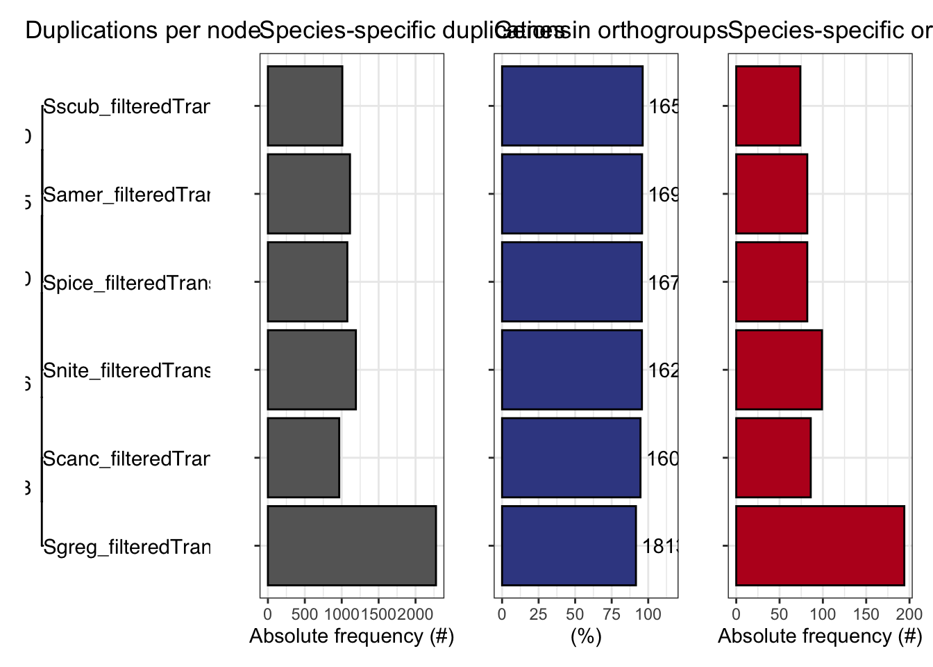
ortho_stats$stats

                    Species N_genes N_genes_in_OGs Perc_genes_in_OGs N_ssOGs
1 Samer_filteredTranscripts   17661          16918              95.8      82
2 Scanc_filteredTranscripts   16906          16008              94.7      86
3 Sgreg_filteredTranscripts   19798          18139              91.6     194
4 Snite_filteredTranscripts   16935          16215              95.7      99
5 Spice_filteredTranscripts   17489          16722              95.6      82
6 Sscub_filteredTranscripts   17236          16588              96.2      74
  N_genes_in_ssOGs Perc_genes_in_ssOGs Dups
1              515                 2.9 1112
2              364                 2.2  966
3              721                 3.6 2277
4              612                 3.6 1192
5              393                 2.2 1076
6              435                 2.5 1008

tree <- treeio::read.tree(file.path(ortho_dir, "Species_Tree/SpeciesTree_rooted_node_labels.txt"))
#tree$tip.label

#custom plot_species
plot_species_tree <- function(tree = NULL, xlim = c(0, 2), stats_list = NULL, custom_labels = NULL) {
    # Basic tree plot with customized theme
    p <- ggtree(tree) +
        xlim(xlim) +
        theme_tree() +  # Use a clean theme
        ggtitle("Species Tree with Duplications") +  # Set a title
        theme(plot.title = element_text(hjust = 0.5))  # Center the title

    # Customize tip labels if provided
    if (!is.null(custom_labels)) {
        # Ensure length of custom_labels matches the number of tree tips
        if (length(custom_labels) == length(tree$tip.label)) {
            p <- p + geom_tiplab(aes(label = custom_labels), size = 4, fontface = "bold.italic", color = "darkblue")
        } else {
            stop("Length of custom_labels must match the number of tip labels in the tree.")
        }
    } else {
        # Default tip labels if no custom labels are provided
        p <- p + geom_tiplab(size = 4, fontface = "bold.italic", color = "darkblue")
    }

    if (!is.null(stats_list)) {
        # Extract duplications
        dups <- stats_list$duplications
        dups <- dups[dups$Node %in% tree$tip.label, ]  # Filter for relevant nodes
        names(dups) <- c("label", "dups")

        # Check for matching nodes
        if (nrow(dups) > 0) {
            p$data <- merge(p$data, dups, by.x = "label", by.y = "label", all.x = TRUE)
            
            # Add duplications to the plot with larger text
            p <- p +
                ggtree::geom_text2(
                    aes(label = .data$dups),
                    hjust = 1.3, vjust = -0.5,
                    size = 5, color = "red"  # Customize size and color of duplication labels
                ) +
                labs(subtitle = "Number of Duplications per Node")  # Subtitle for clarity
        } else {
            message("No matching nodes found for duplications.")
        }
    }

    # Add circles around the nodes
    p <- p + geom_point(size = 2, shape = 21, color = "black", fill = "black")  # Circle around nodes

    return(p)
}


# Plotting the tree
labels6 <- c("Schistocerca gregaria", "Schistocerca piceifrons", "Schistocerca americana", "Schistocerca serialis cubense", "Schistocerca cancellata", "Schistocerca nitens")

# Call the custom plot function with your species tree, stats, and custom labels
p<- plot_species_tree(tree, xlim = c(0, 1.5), stats_list = ortho_stats)

plot_duplications(ortho_stats)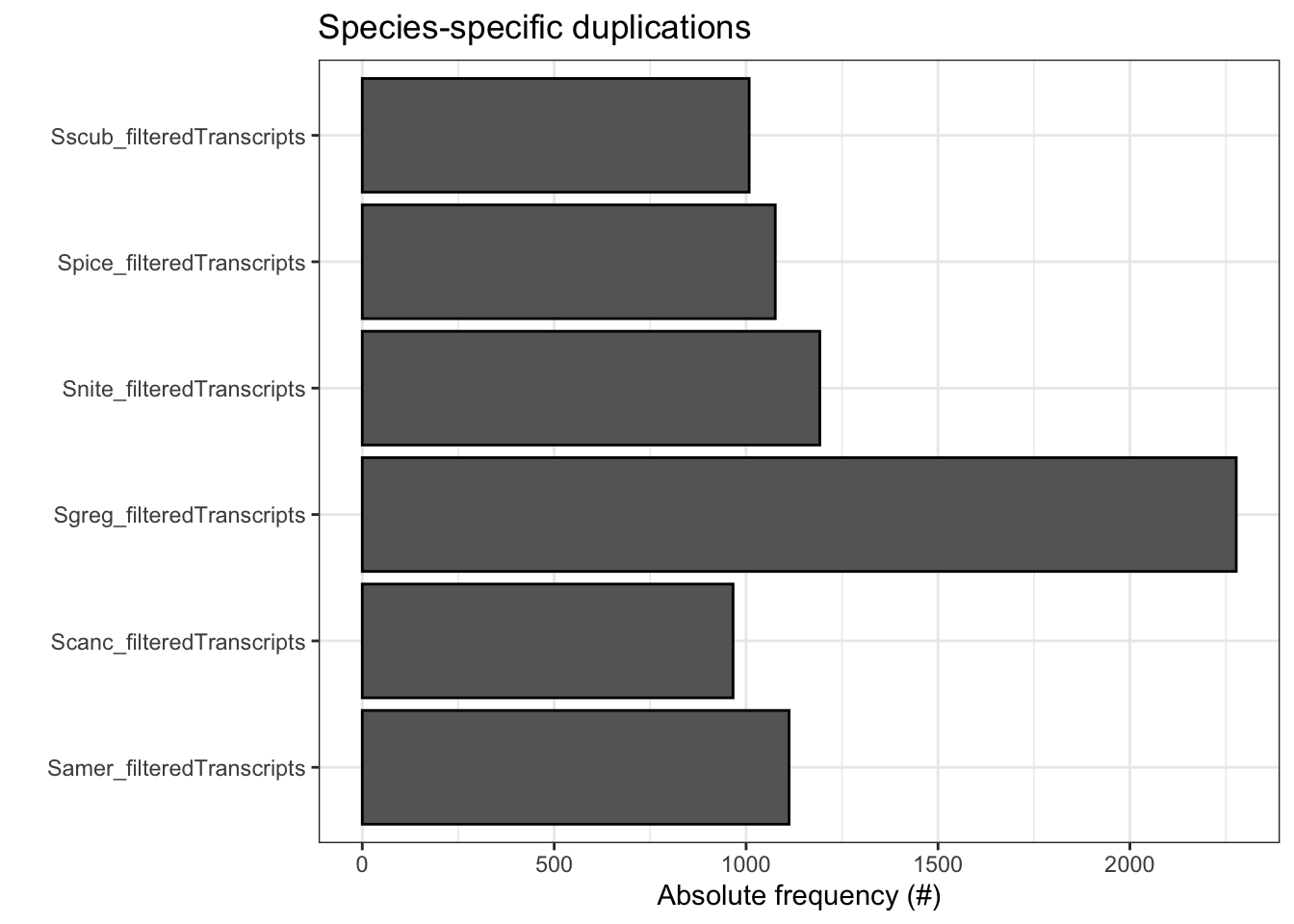

Past versions of "orthofinder cogeqc-1.png"

Version	Author	Date
db8b525	Maeva TECHER	2025-02-06
b80db34	Maeva TECHER	2025-01-13
3fa8e62	Maeva TECHER	2024-11-09

plot_genes_in_ogs(ortho_stats)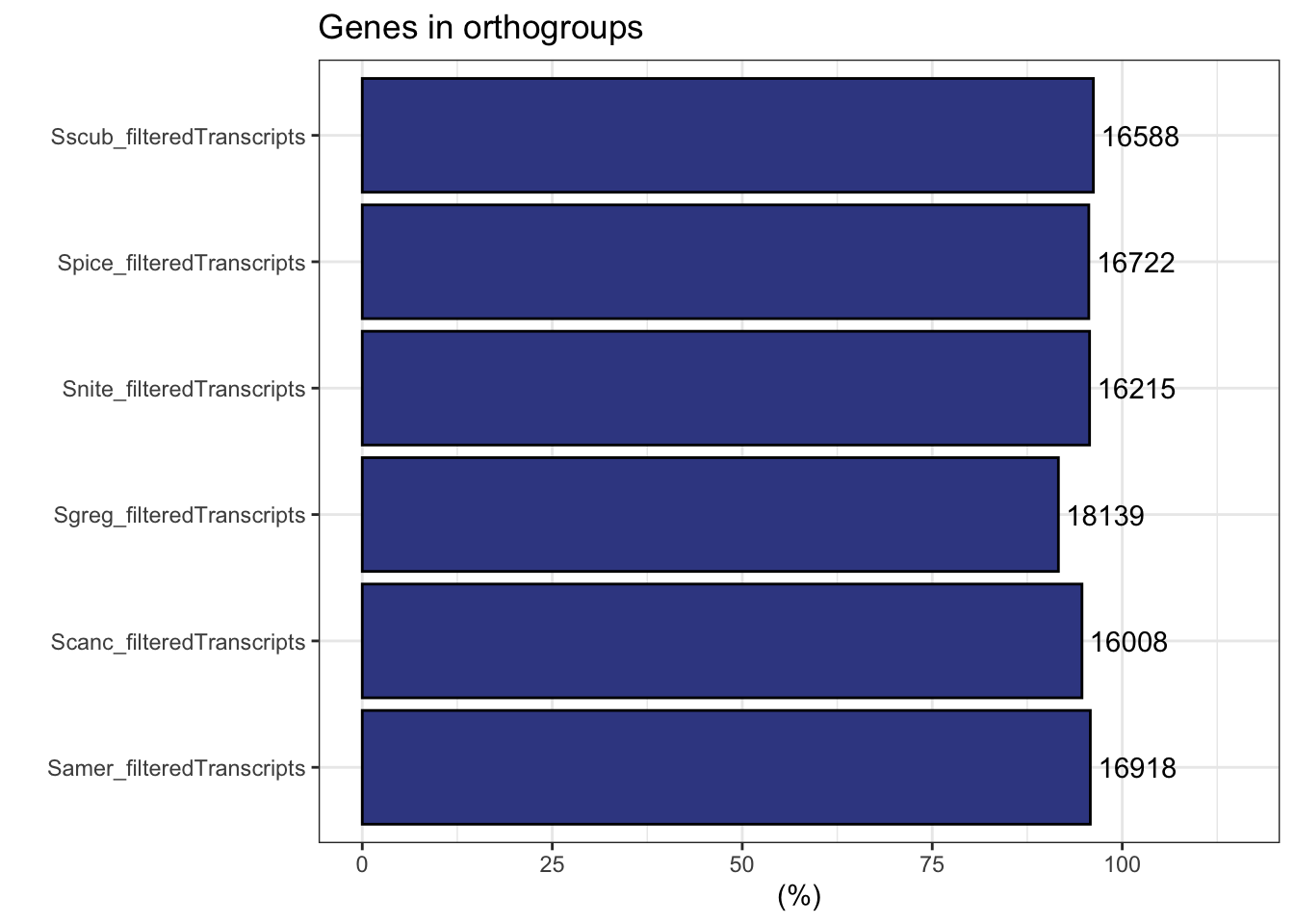

Past versions of "orthofinder cogeqc-2.png"

Version	Author	Date
db8b525	Maeva TECHER	2025-02-06
b80db34	Maeva TECHER	2025-01-13
3fa8e62	Maeva TECHER	2024-11-09

plot_species_specific_ogs(ortho_stats)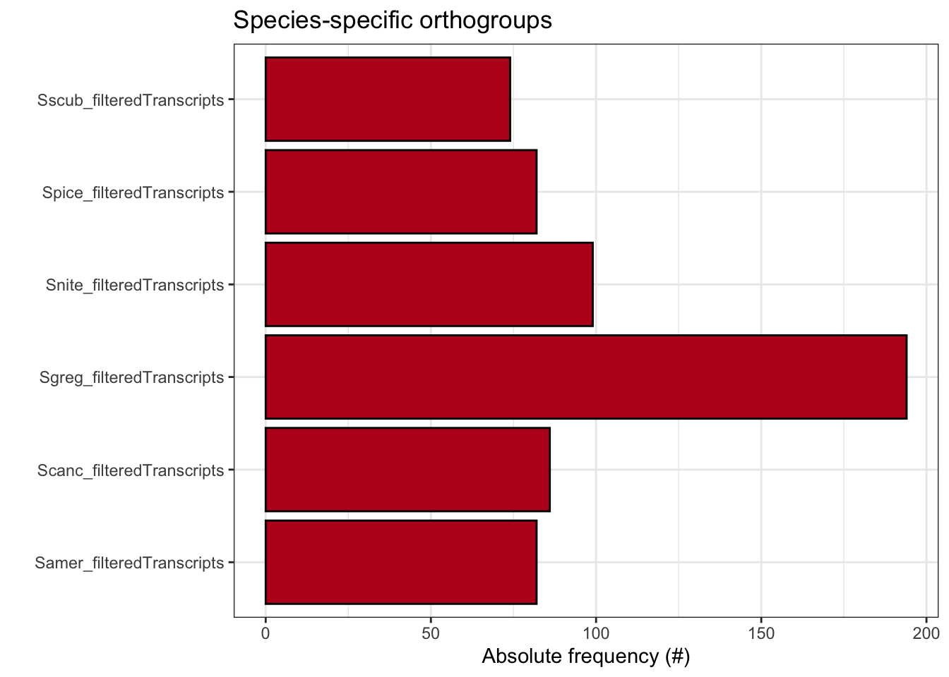

Past versions of "orthofinder cogeqc-3.png"

Version	Author	Date
db8b525	Maeva TECHER	2025-02-06
b80db34	Maeva TECHER	2025-01-13
3fa8e62	Maeva TECHER	2024-11-09

plot_orthofinder_stats(
  tree = tree, 
  xlim = c(-0.1, 2),
  stats_list = ortho_stats
)

Past versions of "orthofinder cogeqc-4.png"

Version	Author	Date
db8b525	Maeva TECHER	2025-02-06
b80db34	Maeva TECHER	2025-01-13
3fa8e62	Maeva TECHER	2024-11-09

plot_og_overlap(ortho_stats)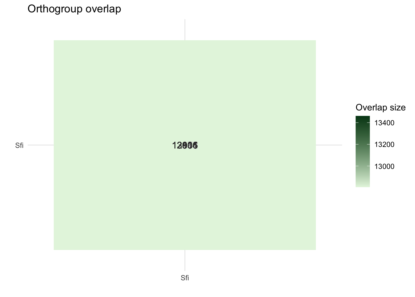

Past versions of "orthofinder cogeqc-5.png"

Version	Author	Date
db8b525	Maeva TECHER	2025-02-06
b80db34	Maeva TECHER	2025-01-13
3fa8e62	Maeva TECHER	2024-11-09

plot_og_sizes(orthogroups)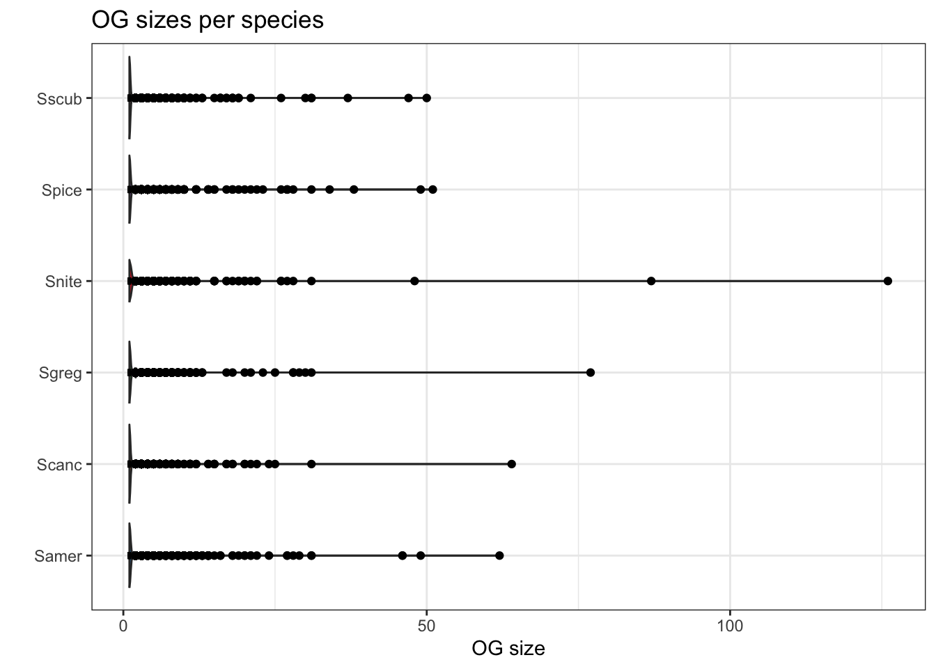

Past versions of "orthofinder cogeqc-6.png"

Version	Author	Date
db8b525	Maeva TECHER	2025-02-06
b80db34	Maeva TECHER	2025-01-13
3fa8e62	Maeva TECHER	2024-11-09

plot_og_sizes(orthogroups, log = TRUE)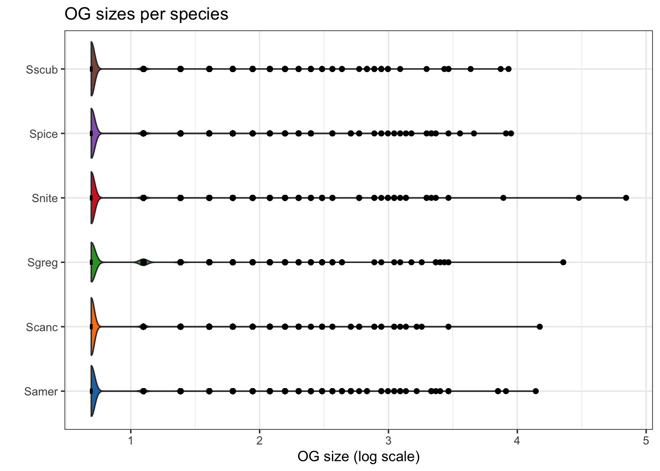 

Past versions of "orthofinder cogeqc-7.png"

Version	Author	Date
db8b525	Maeva TECHER	2025-02-06
b80db34	Maeva TECHER	2025-01-13
3fa8e62	Maeva TECHER	2024-11-09

library(ggplot2)
library(dplyr)
library(tidyr)
library(stringr)
library(tibble)

# Set the base directory for your Orthofinder results
ortho_dir <- "/Users/maevatecher/Documents/GitHub/locust-comparative-genomics/data/orthofinder/Schistocerca/Results_I2/"

dResults <- paste0(ortho_dir, "Comparative_Genomics_Statistics/")
files <- c(
  "OrthologuesStats_one-to-one.tsv",
  "OrthologuesStats_one-to-many.tsv",
  "OrthologuesStats_many-to-one.tsv",
  "OrthologuesStats_many-to-many.tsv"
)

# === Function to Read and Process Data ===
read_data_matrix <- function(file_path) {
  data <- read.delim(file_path, check.names = FALSE, row.names = 1)
  return(as.matrix(data))
}

# === Load Data from Files ===
d11 <- read_data_matrix(paste0(dResults, files[1]))
d1m <- read_data_matrix(paste0(dResults, files[2]))
dm1 <- read_data_matrix(paste0(dResults, files[3]))
dmm <- read_data_matrix(paste0(dResults, files[4]))

# === Schistocerca Species Selection and Order ===
species <- c(
  "Sscub_filteredTranscripts",  # cubense
  "Samer_filteredTranscripts",  # americana
  "Spice_filteredTranscripts",  # piceifrons
  "Scanc_filteredTranscripts",  # cancellata
  "Snite_filteredTranscripts",  # nitens
  "Sgreg_filteredTranscripts"   # gregaria
)

# === Map Species to Readable Labels ===
species_labels <- c(
  "Sscub_filteredTranscripts" = "cubense",
  "Samer_filteredTranscripts" = "americana",
  "Spice_filteredTranscripts" = "piceifrons",
  "Scanc_filteredTranscripts" = "cancellata",
  "Snite_filteredTranscripts" = "nitens",
  "Sgreg_filteredTranscripts" = "gregaria"
)

# === Update Row Names ===
rownames(d11) <- species
rownames(d1m) <- species
rownames(dm1) <- species
rownames(dmm) <- species

# === Function to Prepare Data (Self-Comparison Blank) ===
combine_data <- function(d11, d1m, dm1, dmm, species, species_to_plot) {
  isp <- which(species == species_to_plot)
  dtot <- d11 + d1m + dm1 + dmm
  
  data <- data.frame(
    Species = species,
    `1:1` = ifelse(species == species_to_plot, 0, d11[isp, ] / dtot[isp, ] * 100),
    `1:many` = ifelse(species == species_to_plot, 0, d1m[isp, ] / dtot[isp, ] * 100),
    `many:1` = ifelse(species == species_to_plot, 0, dm1[isp, ] / dtot[isp, ] * 100),
    `many:many` = ifelse(species == species_to_plot, 0, dmm[isp, ] / dtot[isp, ] * 100)
  )
  
  return(data)
}

# === Function to Create and Save Stacked Bar Plot (Vertical) ===
create_plot <- function(data, species_to_plot, output_dir = ortho_dir) {
  data_long <- data %>%
    pivot_longer(
      cols = -Species,
      names_to = "Relationship",
      values_to = "Proportion"
    )
  
  # Rename relationships to match expected levels
  data_long$Relationship <- str_replace_all(data_long$Relationship, c(
    "X1.1" = "1:1",
    "X1.many" = "1:many",
    "many.1" = "many:1",
    "many.many" = "many:many"
  ))
  
  # Ensure Relationship column is a factor with consistent levels
  data_long$Relationship <- factor(
    data_long$Relationship,
    levels = c("1:1", "1:many", "many:1", "many:many")
  )
  
  # Set Custom Species Order
  data_long$Species <- factor(data_long$Species, levels = species, labels = species_labels)

  # Generate the Plot
  plot <- ggplot(data_long, aes(x = Species, y = Proportion, fill = Relationship)) +
    geom_bar(stat = "identity", position = "stack") +
    scale_fill_manual(
      values = c(
        `1:1` = "forestgreen",
        `1:many` = "orange",
        `many:1` = "purple",
        `many:many` = "black"
      )
    ) +
    labs(
      title = paste("Orthologue multiplicty vs", species_labels[species_to_plot]),
      x = "Species",
      y = "Proportion (%)",
      fill = "Relationship Type"
    ) +
    theme_minimal() +
    theme(
      axis.text.x = element_text(angle = 45, hjust = 1),
      axis.title.x = element_text(size = 12),
      axis.title.y = element_text(size = 12)
    )+
    coord_flip()
  
  # Save the Plot
  output_file <- paste0(output_dir, "VerticalStackedBar_", species_labels[species_to_plot], ".pdf")
  ggsave(output_file, plot = plot, width = 10, height = 6)
  cat("Plot saved as:", output_file, "\n")
}

# === Generate Vertical Plots for Each Schistocerca Species ===
output_dir <- paste0(ortho_dir, "Plots_Schistocerca/")  # Specify output directory
dir.create(output_dir, showWarnings = FALSE)

for (species_to_plot in species) {
  data <- combine_data(d11, d1m, dm1, dmm, species, species_to_plot)
  create_plot(data, species_to_plot, output_dir)
}

Plot saved as: /Users/maevatecher/Documents/GitHub/locust-comparative-genomics/data/orthofinder/Schistocerca/Results_I2/Plots_Schistocerca/VerticalStackedBar_cubense.pdf 

Plot saved as: /Users/maevatecher/Documents/GitHub/locust-comparative-genomics/data/orthofinder/Schistocerca/Results_I2/Plots_Schistocerca/VerticalStackedBar_americana.pdf 

Plot saved as: /Users/maevatecher/Documents/GitHub/locust-comparative-genomics/data/orthofinder/Schistocerca/Results_I2/Plots_Schistocerca/VerticalStackedBar_piceifrons.pdf 

Plot saved as: /Users/maevatecher/Documents/GitHub/locust-comparative-genomics/data/orthofinder/Schistocerca/Results_I2/Plots_Schistocerca/VerticalStackedBar_cancellata.pdf 

Plot saved as: /Users/maevatecher/Documents/GitHub/locust-comparative-genomics/data/orthofinder/Schistocerca/Results_I2/Plots_Schistocerca/VerticalStackedBar_nitens.pdf 

Plot saved as: /Users/maevatecher/Documents/GitHub/locust-comparative-genomics/data/orthofinder/Schistocerca/Results_I2/Plots_Schistocerca/VerticalStackedBar_gregaria.pdf 

library(readr)

# rename for future merging
names(orthogroups)[names(orthogroups) == "Gene"] <- "protein_id"
orthogroups <- orthogroups %>%
  mutate(protein_id = str_remove(protein_id, "_p[1-7]$"))

# Optional if you did not rename fasta sequence before
#orthogroups$Species <- gsub("_filteredproteome", "", orthogroups$SpeciesID)

# Export the table to  tab-separated text file (you can change the delimiter if needed)
output_file <- file.path(ortho_dir, "Orthogroups_Schistocerca_Jan2025.txt")

# Write the transformed data to the file
write.table(orthogroups, 
            file = output_file, 
            sep = "\t", 
            quote = FALSE, 
            row.names = FALSE)

proteingene_path <- file.path(ortho_dir, "../../../list/allspecies_protein2geneid.tsv") 
proteingeneid <- read_tsv(proteingene_path, col_names = TRUE ) 
head(proteingeneid)

# A tibble: 6 × 4
  protein_id     GeneID       Description                                Species
  <chr>          <chr>        <chr>                                      <chr>  
1 XP_047114676.1 LOC124794980 piggyBac transposable element-derived pro… Schist…
2 XP_047114773.1 LOC124795035 piggyBac transposable element-derived pro… Schist…
3 XP_047117829.1 LOC124798450 uncharacterized protein LOC124798450       Schist…
4 XP_047118606.1 LOC124799109 RNA-binding protein 25-like                Schist…
5 XP_047118853.1 LOC124799306 molybdenum cofactor biosynthesis protein … Schist…
6 XP_047118904.1 LOC124799809 molybdenum cofactor biosynthesis protein … Schist…

biotype_path <- file.path(ortho_dir, "../../../list/13polyneoptera_geneid_ncbi.csv") 
biotypeid <- read_csv(biotype_path, col_names = TRUE ) 
head(biotypeid)

# A tibble: 6 × 10
  Accession Begin   End Description Symbol GeneID GeneType Transcripts_accession
  <chr>     <dbl> <dbl> <chr>       <chr>  <chr>  <chr>    <chr>                
1 NC_06468…     1    66 tRNA-Ile    trnI   LOC73… tRNA     <NA>                 
2 NC_06468…    70   138 tRNA-Gln    trnQ   LOC73… tRNA     <NA>                 
3 NC_06468…   138   206 tRNA-Met    trnM   LOC73… tRNA     <NA>                 
4 NC_06468…   207  1227 NADH dehyd… ND2    LOC73… protein… <NA>                 
5 NC_06468…  1228  1295 tRNA-Trp    trnW   LOC73… tRNA     <NA>                 
6 NC_06468…  1288  1350 tRNA-Cys    trnC   LOC73… tRNA     <NA>                 
# ℹ 2 more variables: protein_id <chr>, Species <chr>

# Ensure GeneID is treated as a character to avoid mismatches
proteinorthotable <- left_join(orthogroups, proteingeneid, by = "protein_id")
final_orthotable <- left_join(biotypeid, proteinorthotable[, c("Orthogroup","SpeciesID", "GeneID")],  by = "GeneID")

output_file <- file.path(ortho_dir, "Orthogroups_genesproteinbiotype_Schistocerca_Jan2025.csv")

# Write the table with proper quoting and no row names
write.table(final_orthotable, file = output_file, sep = ",", quote = TRUE, row.names = FALSE, col.names = TRUE)

There we have it, the final table with all the corresponding IDs. This table is too big and have all species in it, so we want to reduce to only single copy orthologs and remove entries with other species than Schistocerca for now.

# Filter the final_orthotable to keep only rows with species 'Schistocerca'
filtered_final_orthotable <- final_orthotable %>%
  filter(Species %in% c("Schistocerca gregaria", "Schistocerca piceifrons", "Schistocerca americana", "Schistocerca cancellata", "Schistocerca serialis cubense", "Schistocerca nitens"))


# Optionally, save the filtered data
#output_file <- file.path(ortho_dir, "Orthogroups_genesprotein_Schisto_Jan2025.txt")
#write.table(filtered_final_orthotable, file = output_file, sep = "\t", quote = FALSE, row.names = FALSE)

# Step 1: Read the single copy orthologs table
single_copy_orthologs_path <- file.path(ortho_dir, "Orthogroups/Orthogroups_SingleCopyOrthologues.txt")
single_copy_orthologs <- read.table(single_copy_orthologs_path, header = FALSE, stringsAsFactors = FALSE)

# Step 2: Ensure the column name for orthogroups matches in both data frames
# If necessary, rename the column in single_copy_orthologs to match
colnames(single_copy_orthologs) <- c("Orthogroup")  # Replace with the actual name if different

# Step 3: Perform the intersection
scopy_final_orthotable <- final_orthotable[final_orthotable$Orthogroup %in% single_copy_orthologs$Orthogroup, ]

# Step 4: Optionally, save the filtered table
output_file <- file.path(ortho_dir, "SingleCopyOrthogroups_genesprotein_6species_Jan2025.txt")
write.table(scopy_final_orthotable, file = output_file, sep = "\t", quote = FALSE, row.names = FALSE)

Polyneoptera

library(cogeqc)
library(ggtree)
library(treeio)
library(dplyr)
library(ggplot2)

# Set the base directory for your Orthofinder results
ortho_dir <- "/Users/maevatecher/Documents/GitHub/locust-comparative-genomics/data/orthofinder/Polyneoptera/Results_I2/"

# Load the orthogroup file
orthogroups <- read_orthogroups(file.path(ortho_dir, "Orthogroups/Orthogroups_reprocessed.tsv"))
# Remove "_filteredTranscripts" from the Species column
orthogroups <- orthogroups %>%
  mutate(SpeciesID = str_replace(Species, "_filteredTranscripts", "")) %>%  # Clean Species name
  select(Orthogroup, SpeciesID, Gene)  # Rename and keep relevant columns

# Load the directory with the actual stats from the Orthofinder run
ortho_stats <- read_orthofinder_stats(file.path(ortho_dir, "Comparative_Genomics_Statistics"))
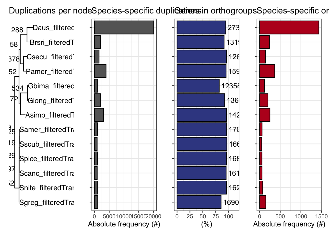
ortho_stats$stats

                     Species N_genes N_genes_in_OGs Perc_genes_in_OGs N_ssOGs
1  Asimp_filteredTranscripts   14865          14272              96.0     250
2  Brsri_filteredTranscripts   14447          13195              91.3     237
3  Csecu_filteredTranscripts   13169          12653              96.1     142
4   Daus_filteredTranscripts   28958          27396              94.6    1437
5  Gbima_filteredTranscripts   15112          12358              81.8     115
6  Glong_filteredTranscripts   14729          13604              92.4     202
7  Pamer_filteredTranscripts   16749          15946              95.2     368
8  Samer_filteredTranscripts   17661          17008              96.3      60
9  Scanc_filteredTranscripts   16906          16106              95.3      58
10 Sgreg_filteredTranscripts   19798          16902              85.4     151
11 Snite_filteredTranscripts   16935          16262              96.0      77
12 Spice_filteredTranscripts   17489          16809              96.1      56
13 Sscub_filteredTranscripts   17236          16661              96.7      53
   N_genes_in_ssOGs Perc_genes_in_ssOGs  Dups
1              1565                10.5  3089
2              1018                 7.0  2083
3               679                 5.2  1562
4             13979                48.3 20104
5               335                 2.2  1092
6              1010                 6.9  2006
7              2441                14.6  3924
8               338                 1.9  1022
9               280                 1.7   935
10              529                 2.7  1131
11              501                 3.0  1085
12              281                 1.6  1012
13              280                 1.6   918

tree <- treeio::read.tree(file.path(ortho_dir, "Species_Tree/SpeciesTree_rooted_node_labels.txt"))
#tree$tip.label

#custom plot_species
plot_species_tree <- function(tree = NULL, xlim = c(0, 2), stats_list = NULL, custom_labels = NULL) {
    # Basic tree plot with customized theme
    p <- ggtree(tree) +
        xlim(xlim) +
        theme_tree() +  # Use a clean theme
        ggtitle("Species Tree with Duplications") +  # Set a title
        theme(plot.title = element_text(hjust = 0.5))  # Center the title

    # Customize tip labels if provided
    if (!is.null(custom_labels)) {
        # Ensure length of custom_labels matches the number of tree tips
        if (length(custom_labels) == length(tree$tip.label)) {
            p <- p + geom_tiplab(aes(label = custom_labels), size = 4, fontface = "bold.italic", color = "darkblue")
        } else {
            stop("Length of custom_labels must match the number of tip labels in the tree.")
        }
    } else {
        # Default tip labels if no custom labels are provided
        p <- p + geom_tiplab(size = 4, fontface = "bold.italic", color = "darkblue")
    }

    if (!is.null(stats_list)) {
        # Extract duplications
        dups <- stats_list$duplications
        dups <- dups[dups$Node %in% tree$tip.label, ]  # Filter for relevant nodes
        names(dups) <- c("label", "dups")

        # Check for matching nodes
        if (nrow(dups) > 0) {
            p$data <- merge(p$data, dups, by.x = "label", by.y = "label", all.x = TRUE)
            
            # Add duplications to the plot with larger text
            p <- p +
                ggtree::geom_text2(
                    aes(label = .data$dups),
                    hjust = 1.3, vjust = -0.5,
                    size = 5, color = "red"  # Customize size and color of duplication labels
                ) +
                labs(subtitle = "Number of Duplications per Node")  # Subtitle for clarity
        } else {
            message("No matching nodes found for duplications.")
        }
    }

    # Add circles around the nodes
    p <- p + geom_point(size = 2, shape = 21, color = "black", fill = "black")  # Circle around nodes

    return(p)
}


# Call the custom plot function with your species tree, stats, and custom labels
p<- plot_species_tree(tree, xlim = c(0, 1.5), stats_list = ortho_stats)

plot_duplications(ortho_stats)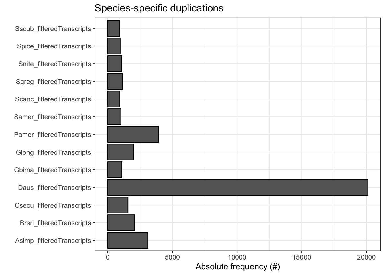

Past versions of "orthofinder cogeqc2-1.png"

Version	Author	Date
db8b525	Maeva TECHER	2025-02-06
b80db34	Maeva TECHER	2025-01-13

plot_genes_in_ogs(ortho_stats)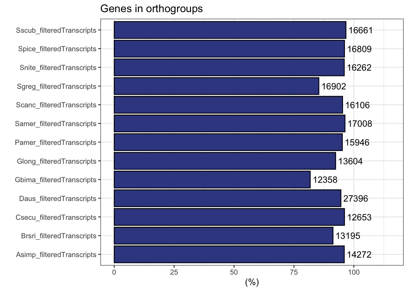

Past versions of "orthofinder cogeqc2-2.png"

Version	Author	Date
db8b525	Maeva TECHER	2025-02-06
b80db34	Maeva TECHER	2025-01-13

plot_species_specific_ogs(ortho_stats)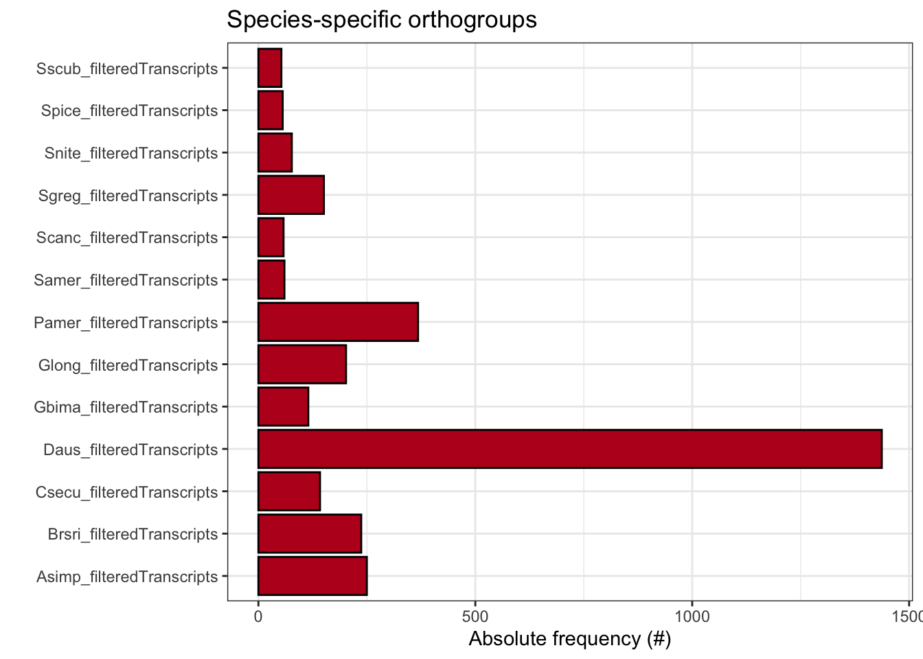

Past versions of "orthofinder cogeqc2-3.png"

Version	Author	Date
db8b525	Maeva TECHER	2025-02-06
b80db34	Maeva TECHER	2025-01-13

plot_orthofinder_stats(
  tree = tree, 
  xlim = c(-0.1, 2),
  stats_list = ortho_stats
)

Past versions of "orthofinder cogeqc2-4.png"

Version	Author	Date
db8b525	Maeva TECHER	2025-02-06
b80db34	Maeva TECHER	2025-01-13

plot_og_overlap(ortho_stats)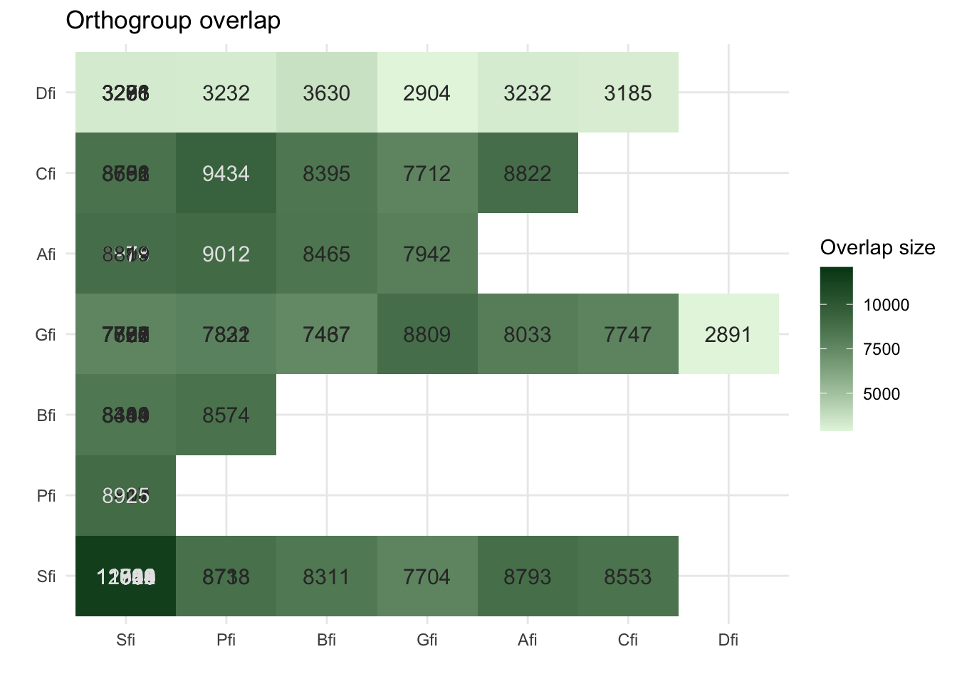

Past versions of "orthofinder cogeqc2-5.png"

Version	Author	Date
db8b525	Maeva TECHER	2025-02-06
b80db34	Maeva TECHER	2025-01-13

plot_og_sizes(orthogroups)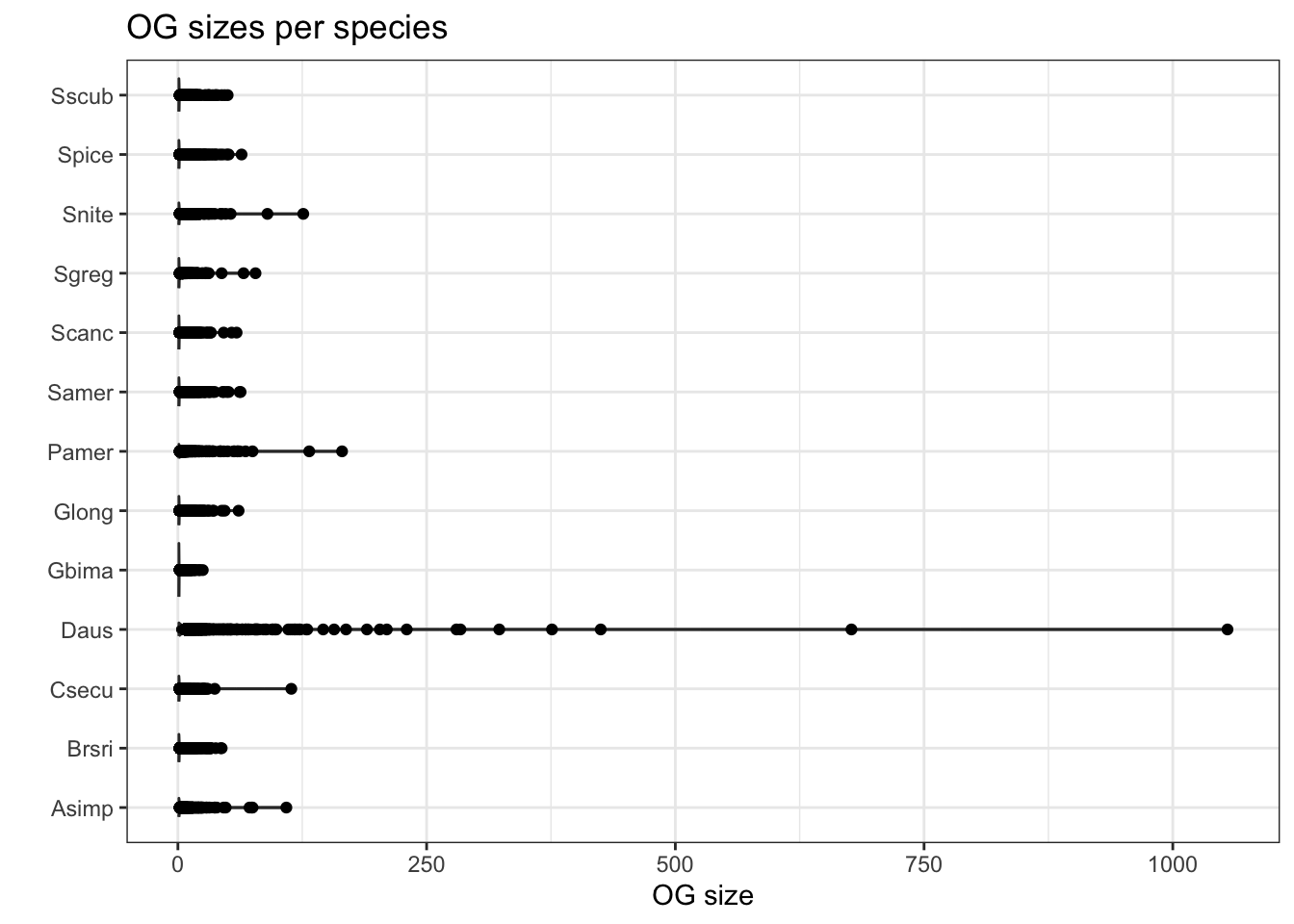

Past versions of "orthofinder cogeqc2-6.png"

Version	Author	Date
db8b525	Maeva TECHER	2025-02-06
b80db34	Maeva TECHER	2025-01-13

plot_og_sizes(orthogroups, log = TRUE)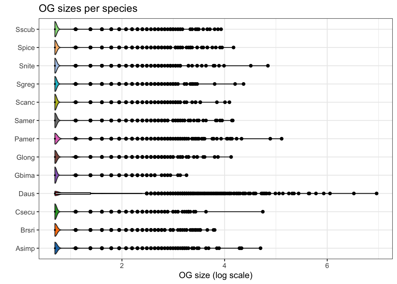 

Past versions of "orthofinder cogeqc2-7.png"

Version	Author	Date
db8b525	Maeva TECHER	2025-02-06
b80db34	Maeva TECHER	2025-01-13

# Set the base directory for your Orthofinder results
ortho_dir <- "/Users/maevatecher/Documents/GitHub/locust-comparative-genomics/data/orthofinder/Polyneoptera/Results_I2/"

dResults <- paste0(ortho_dir, "Comparative_Genomics_Statistics/")
files <- c(
  "OrthologuesStats_one-to-one.tsv",
  "OrthologuesStats_one-to-many.tsv",
  "OrthologuesStats_many-to-one.tsv",
  "OrthologuesStats_many-to-many.tsv"
)

# === Function to Read and Process Data ===
read_data_matrix <- function(file_path) {
  data <- read.delim(file_path, check.names = FALSE, row.names = 1)
  return(as.matrix(data))
}

# === Load Data from Files ===
d11 <- read_data_matrix(paste0(dResults, files[1]))
d1m <- read_data_matrix(paste0(dResults, files[2]))
dm1 <- read_data_matrix(paste0(dResults, files[3]))
dmm <- read_data_matrix(paste0(dResults, files[4]))

# === Schistocerca Species Selection and Order ===
species <- c(
  "Sscub_filteredTranscripts",  # cubense
  "Samer_filteredTranscripts",  # americana
  "Spice_filteredTranscripts",  # piceifrons
  "Scanc_filteredTranscripts",  # cancellata
  "Snite_filteredTranscripts",  # nitens
  "Sgreg_filteredTranscripts",  # gregaria
  "Gbima_filteredTranscripts",  # Gryllus bimaculatus
  "Glong_filteredTranscripts",  # Gryllus longicornis
  "Asimp_filteredTranscripts",  # A. simplex (Stick Insect)
  "Brsri_filteredTranscripts",  # B. rossius (Stick Insect)
  "Daus_filteredTranscripts",   # D. australis (Lord Howe Island Stick Insect)
  "Pamer_filteredTranscripts",  # P. americana (American Cockroach)
  "Csecu_filteredTranscripts"   # C. secundus (Drywood Termite)
)

# === Map Species to Readable Labels ===
species_labels <- c(
  "Sscub_filteredTranscripts" = "cubense",
  "Samer_filteredTranscripts" = "americana",
  "Spice_filteredTranscripts" = "piceifrons",
  "Scanc_filteredTranscripts" = "cancellata",
  "Snite_filteredTranscripts" = "nitens",
  "Sgreg_filteredTranscripts" = "gregaria",
  "Gbima_filteredTranscripts" = "G. bimaculatus",
  "Glong_filteredTranscripts" = "G. longicornis",
  "Asimp_filteredTranscripts" = "A. simplex",
  "Brsri_filteredTranscripts" = "B. rossius",
  "Daus_filteredTranscripts" = "D. australis",
  "Pamer_filteredTranscripts" = "P. americana",
  "Csecu_filteredTranscripts" = "C. secundus"
)

# === Update Row Names ===
rownames(d11) <- species
rownames(d1m) <- species
rownames(dm1) <- species
rownames(dmm) <- species

# === Function to Prepare Data (Self-Comparison Blank) ===
combine_data <- function(d11, d1m, dm1, dmm, species, species_to_plot) {
  isp <- which(species == species_to_plot)
  dtot <- d11 + d1m + dm1 + dmm
  
  data <- data.frame(
    Species = species,
    `1:1` = ifelse(species == species_to_plot, 0, d11[isp, ] / dtot[isp, ] * 100),
    `1:many` = ifelse(species == species_to_plot, 0, d1m[isp, ] / dtot[isp, ] * 100),
    `many:1` = ifelse(species == species_to_plot, 0, dm1[isp, ] / dtot[isp, ] * 100),
    `many:many` = ifelse(species == species_to_plot, 0, dmm[isp, ] / dtot[isp, ] * 100)
  )
  
  return(data)
}

# === Function to Create and Save Stacked Bar Plot (Vertical) ===
create_plot <- function(data, species_to_plot, output_dir = ortho_dir) {
  data_long <- data %>%
    pivot_longer(
      cols = -Species,
      names_to = "Relationship",
      values_to = "Proportion"
    )
  
  # Rename relationships to match expected levels
  data_long$Relationship <- str_replace_all(data_long$Relationship, c(
    "X1.1" = "1:1",
    "X1.many" = "1:many",
    "many.1" = "many:1",
    "many.many" = "many:many"
  ))
  
  # Ensure Relationship column is a factor with consistent levels
  data_long$Relationship <- factor(
    data_long$Relationship,
    levels = c("1:1", "1:many", "many:1", "many:many")
  )
  
  # Set Custom Species Order
  data_long$Species <- factor(data_long$Species, levels = species, labels = species_labels)

  # Generate the Plot
  plot <- ggplot(data_long, aes(x = Species, y = Proportion, fill = Relationship)) +
    geom_bar(stat = "identity", position = "stack") +
    scale_fill_manual(
      values = c(
        `1:1` = "forestgreen",
        `1:many` = "orange",
        `many:1` = "purple",
        `many:many` = "black"
      )
    ) +
    labs(
      title = paste("Orthologue multiplicty vs", species_labels[species_to_plot]),
      x = "Species",
      y = "Proportion (%)",
      fill = "Relationship Type"
    ) +
    theme_minimal() +
    theme(
      axis.text.x = element_text(angle = 45, hjust = 1),
      axis.title.x = element_text(size = 12),
      axis.title.y = element_text(size = 12)
    )+
    coord_flip()
  
  # Save the Plot
  output_file <- paste0(output_dir, "VerticalStackedBar_", species_labels[species_to_plot], ".pdf")
  ggsave(output_file, plot = plot, width = 10, height = 6)
  cat("Plot saved as:", output_file, "\n")
}

# === Generate Vertical Plots for Each Schistocerca Species ===
output_dir <- paste0(ortho_dir, "Plots_Polyneoptera/")  # Specify output directory
dir.create(output_dir, showWarnings = FALSE)

for (species_to_plot in species) {
  data <- combine_data(d11, d1m, dm1, dmm, species, species_to_plot)
  create_plot(data, species_to_plot, output_dir)
}

Plot saved as: /Users/maevatecher/Documents/GitHub/locust-comparative-genomics/data/orthofinder/Polyneoptera/Results_I2/Plots_Polyneoptera/VerticalStackedBar_cubense.pdf 

Plot saved as: /Users/maevatecher/Documents/GitHub/locust-comparative-genomics/data/orthofinder/Polyneoptera/Results_I2/Plots_Polyneoptera/VerticalStackedBar_americana.pdf 

Plot saved as: /Users/maevatecher/Documents/GitHub/locust-comparative-genomics/data/orthofinder/Polyneoptera/Results_I2/Plots_Polyneoptera/VerticalStackedBar_piceifrons.pdf 

Plot saved as: /Users/maevatecher/Documents/GitHub/locust-comparative-genomics/data/orthofinder/Polyneoptera/Results_I2/Plots_Polyneoptera/VerticalStackedBar_cancellata.pdf 

Plot saved as: /Users/maevatecher/Documents/GitHub/locust-comparative-genomics/data/orthofinder/Polyneoptera/Results_I2/Plots_Polyneoptera/VerticalStackedBar_nitens.pdf 

Plot saved as: /Users/maevatecher/Documents/GitHub/locust-comparative-genomics/data/orthofinder/Polyneoptera/Results_I2/Plots_Polyneoptera/VerticalStackedBar_gregaria.pdf 

Plot saved as: /Users/maevatecher/Documents/GitHub/locust-comparative-genomics/data/orthofinder/Polyneoptera/Results_I2/Plots_Polyneoptera/VerticalStackedBar_G. bimaculatus.pdf 

Plot saved as: /Users/maevatecher/Documents/GitHub/locust-comparative-genomics/data/orthofinder/Polyneoptera/Results_I2/Plots_Polyneoptera/VerticalStackedBar_G. longicornis.pdf 

Plot saved as: /Users/maevatecher/Documents/GitHub/locust-comparative-genomics/data/orthofinder/Polyneoptera/Results_I2/Plots_Polyneoptera/VerticalStackedBar_A. simplex.pdf 

Plot saved as: /Users/maevatecher/Documents/GitHub/locust-comparative-genomics/data/orthofinder/Polyneoptera/Results_I2/Plots_Polyneoptera/VerticalStackedBar_B. rossius.pdf 

Plot saved as: /Users/maevatecher/Documents/GitHub/locust-comparative-genomics/data/orthofinder/Polyneoptera/Results_I2/Plots_Polyneoptera/VerticalStackedBar_D. australis.pdf 

Plot saved as: /Users/maevatecher/Documents/GitHub/locust-comparative-genomics/data/orthofinder/Polyneoptera/Results_I2/Plots_Polyneoptera/VerticalStackedBar_P. americana.pdf 

Plot saved as: /Users/maevatecher/Documents/GitHub/locust-comparative-genomics/data/orthofinder/Polyneoptera/Results_I2/Plots_Polyneoptera/VerticalStackedBar_C. secundus.pdf 

library(readr)

# rename for future merging
names(orthogroups)[names(orthogroups) == "Gene"] <- "protein_id"
orthogroups <- orthogroups %>%
  mutate(protein_id = str_remove(protein_id, "_p[1-7]$"))
# Optional if you did not rename fasta sequence before
orthogroups$Species <- gsub("_filteredproteome", "", orthogroups$Species)
# Export the table to  tab-separated text file (you can change the delimiter if needed)
output_file <- file.path(ortho_dir, "Orthogroups_13species_Jan2025.txt")

# Write the transformed data to the file
write.table(orthogroups, 
            file = output_file, 
            sep = "\t", 
            quote = FALSE, 
            row.names = FALSE)


proteingene_path <- file.path(ortho_dir, "../../../list/allspecies_protein2geneid.tsv") 
proteingeneid <- read_tsv(proteingene_path, col_names = TRUE ) 
head(proteingeneid)

# A tibble: 6 × 4
  protein_id     GeneID       Description                                Species
  <chr>          <chr>        <chr>                                      <chr>  
1 XP_047114676.1 LOC124794980 piggyBac transposable element-derived pro… Schist…
2 XP_047114773.1 LOC124795035 piggyBac transposable element-derived pro… Schist…
3 XP_047117829.1 LOC124798450 uncharacterized protein LOC124798450       Schist…
4 XP_047118606.1 LOC124799109 RNA-binding protein 25-like                Schist…
5 XP_047118853.1 LOC124799306 molybdenum cofactor biosynthesis protein … Schist…
6 XP_047118904.1 LOC124799809 molybdenum cofactor biosynthesis protein … Schist…

biotype_path <- file.path(ortho_dir, "../../../list/13polyneoptera_geneid_ncbi.csv") 
biotypeid <- read_csv(biotype_path, col_names = TRUE ) 
head(biotypeid)

# A tibble: 6 × 10
  Accession Begin   End Description Symbol GeneID GeneType Transcripts_accession
  <chr>     <dbl> <dbl> <chr>       <chr>  <chr>  <chr>    <chr>                
1 NC_06468…     1    66 tRNA-Ile    trnI   LOC73… tRNA     <NA>                 
2 NC_06468…    70   138 tRNA-Gln    trnQ   LOC73… tRNA     <NA>                 
3 NC_06468…   138   206 tRNA-Met    trnM   LOC73… tRNA     <NA>                 
4 NC_06468…   207  1227 NADH dehyd… ND2    LOC73… protein… <NA>                 
5 NC_06468…  1228  1295 tRNA-Trp    trnW   LOC73… tRNA     <NA>                 
6 NC_06468…  1288  1350 tRNA-Cys    trnC   LOC73… tRNA     <NA>                 
# ℹ 2 more variables: protein_id <chr>, Species <chr>

# Ensure GeneID is treated as a character to avoid mismatches
proteinorthotable <- left_join(orthogroups, proteingeneid, by = "protein_id")
final_orthotable <- left_join(biotypeid, proteinorthotable[, c("Orthogroup","SpeciesID", "GeneID")],  by = "GeneID")

output_file <- file.path(ortho_dir, "Orthogroups_genesproteinbiotype_13species_Jan2025.csv")
# Write the table with proper quoting and no row names
write.table(final_orthotable, file = output_file, sep = ",", quote = TRUE, row.names = FALSE, col.names = TRUE)

There we have it, the final table with all the corresponding IDs. This table is too big and have all species in it, so we want to reduce to only single copy orthologs and remove entries with other species than Schistocerca for now.

# Filter the final_orthotable to keep only rows with species 'Schistocerca'
filtered_final_orthotable <- final_orthotable %>%
  filter(Species %in% c("Schistocerca gregaria", "Schistocerca piceifrons", "Schistocerca americana", "Schistocerca cancellata", "Schistocerca serialis cubense", "Schistocerca nitens"))


# Optionally, save the filtered data
output_file <- file.path(ortho_dir, "Orthogroups_genesprotein_Schisto_Jan2025.txt")
write.table(filtered_final_orthotable, file = output_file, sep = "\t", quote = FALSE, row.names = FALSE)

# Step 1: Read the single copy orthologs table
single_copy_orthologs_path <- file.path(ortho_dir, "Orthogroups/Orthogroups_SingleCopyOrthologues.txt")
single_copy_orthologs <- read.table(single_copy_orthologs_path, header = FALSE, stringsAsFactors = FALSE)

# Step 2: Ensure the column name for orthogroups matches in both data frames
# If necessary, rename the column in single_copy_orthologs to match
colnames(single_copy_orthologs) <- c("Orthogroup")  # Replace with the actual name if different

# Step 3: Perform the intersection
scopy_final_orthotable <- final_orthotable[final_orthotable$Orthogroup %in% single_copy_orthologs$Orthogroup, ]

# Step 4: Optionally, save the filtered table
output_file <- file.path(ortho_dir, "SingleCopyOrthogroups_genesprotein_13species_Jan2025.txt")
write.table(scopy_final_orthotable, file = output_file, sep = "\t", quote = FALSE, row.names = FALSE)

References

If you use this script, and orthologr please cite:

Drost et al. 2015. Evidence for Active Maintenance of Phylotranscriptomic Hourglass Patterns in Animal and Plant Embryogenesis. Mol. Biol. Evol. 32 (5): 1221-1231. doi:10.1093/molbev/msv012

If you use Transdecoder, please cite it as:

Haas, B., and A. Papanicolaou. “TransDecoder.” (2017).

If you use Orthofinder, please cite it:

OrthoFinder’s orthogroup and ortholog inference are described here:

Emms, D.M., Kelly, S. OrthoFinder: solving fundamental biases in whole genome comparisons dramatically improves orthogroup inference accuracy. Genome Biol 16, 157 (2015).

Emms, D.M., Kelly, S. OrthoFinder: phylogenetic orthology inference for comparative genomics. Genome Biol 20, 238 (2019).

If you use the OrthoFinder species tree then also cite:

Emms D.M. & Kelly S. STRIDE: Species Tree Root Inference from Gene Duplication Events (2017), Mol Biol Evol 34(12): 3267-3278.

Emms D.M. & Kelly S. STAG: Species Tree Inference from All Genes (2018), bioRxiv https://doi.org/10.1101/267914.

Please also cite MAFFT:

K. Katoh, K. Misawa, K. Kuma, and T. Miyata. 2002. MAFFT: a novel method for rapid multiple sequence alignment based on fast Fourier transform. Nucleic Acids Res. 30(14): 3059-3066.

Session information

sessionInfo()

R version 4.4.1 (2024-06-14)
Platform: aarch64-apple-darwin20
Running under: macOS 15.3

Matrix products: default
BLAS:   /Library/Frameworks/R.framework/Versions/4.4-arm64/Resources/lib/libRblas.0.dylib 
LAPACK: /Library/Frameworks/R.framework/Versions/4.4-arm64/Resources/lib/libRlapack.dylib;  LAPACK version 3.12.0

locale:
[1] en_US.UTF-8/en_US.UTF-8/en_US.UTF-8/C/en_US.UTF-8/en_US.UTF-8

time zone: Asia/Tokyo
tzcode source: internal

attached base packages:
[1] stats     graphics  grDevices utils     datasets  methods   base     

other attached packages:
 [1] readr_2.1.5      tibble_3.2.1     tidyr_1.3.1      stringr_1.5.1   
 [5] ggplot2_3.5.1    dplyr_1.1.4      treeio_1.28.0    ggtree_3.12.0   
 [9] cogeqc_1.8.0     kableExtra_1.4.0 knitr_1.49      

loaded via a namespace (and not attached):
 [1] tidyselect_1.2.1        viridisLite_0.4.2       vipor_0.4.7            
 [4] farver_2.1.2            Biostrings_2.72.1       fastmap_1.2.0          
 [7] lazyeval_0.2.2          promises_1.3.2          digest_0.6.37          
[10] lifecycle_1.0.4         tidytree_0.4.6          magrittr_2.0.3         
[13] compiler_4.4.1          rlang_1.1.4             sass_0.4.9             
[16] tools_4.4.1             utf8_1.2.4              igraph_2.1.2           
[19] yaml_2.3.10             labeling_0.4.3          bit_4.5.0.1            
[22] plyr_1.8.9              xml2_1.3.6              aplot_0.2.4            
[25] workflowr_1.7.1         withr_3.0.2             purrr_1.0.2            
[28] BiocGenerics_0.50.0     grid_4.4.1              stats4_4.4.1           
[31] git2r_0.35.0            colorspace_2.1-1        scales_1.3.0           
[34] cli_3.6.3               rmarkdown_2.29          crayon_1.5.3           
[37] ragg_1.3.3              generics_0.1.3          rstudioapi_0.17.1      
[40] tzdb_0.4.0              httr_1.4.7              reshape2_1.4.4         
[43] ggbeeswarm_0.7.2        ape_5.8-1               cachem_1.1.0           
[46] zlibbioc_1.50.0         parallel_4.4.1          ggplotify_0.1.2        
[49] XVector_0.44.0          vctrs_0.6.5             yulab.utils_0.1.9      
[52] jsonlite_1.8.9          hms_1.1.3               gridGraphics_0.5-1     
[55] IRanges_2.38.1          patchwork_1.3.0         S4Vectors_0.42.1       
[58] bit64_4.5.2             beeswarm_0.4.0          systemfonts_1.1.0      
[61] jquerylib_0.1.4         glue_1.8.0              stringi_1.8.4          
[64] gtable_0.3.6            later_1.4.1             GenomeInfoDb_1.40.1    
[67] UCSC.utils_1.0.0        munsell_0.5.1           pillar_1.10.1          
[70] htmltools_0.5.8.1       GenomeInfoDbData_1.2.12 R6_2.5.1               
[73] textshaping_0.4.1       rprojroot_2.0.4         vroom_1.6.5            
[76] evaluate_1.0.3          lattice_0.22-6          httpuv_1.6.15          
[79] ggfun_0.1.8             bslib_0.8.0             Rcpp_1.0.14            
[82] svglite_2.1.3           nlme_3.1-166            whisker_0.4.1          
[85] xfun_0.50               fs_1.6.5                pkgconfig_2.0.3