Gene database tables: Orthologs, Genes under selection, DEGs and RNAi
Maeva Techer
2025-07-01
Last updated: 2025-07-01
Checks: 6 1
Knit directory:
locust-comparative-genomics/
This reproducible R Markdown analysis was created with workflowr (version 1.7.1). The Checks tab describes the reproducibility checks that were applied when the results were created. The Past versions tab lists the development history.
Great! Since the R Markdown file has been committed to the Git repository, you know the exact version of the code that produced these results.
Great job! The global environment was empty. Objects defined in the global environment can affect the analysis in your R Markdown file in unknown ways. For reproduciblity it’s best to always run the code in an empty environment.
The command set.seed(20221025) was run prior to running
the code in the R Markdown file. Setting a seed ensures that any results
that rely on randomness, e.g. subsampling or permutations, are
reproducible.
Great job! Recording the operating system, R version, and package versions is critical for reproducibility.
Nice! There were no cached chunks for this analysis, so you can be confident that you successfully produced the results during this run.
Using absolute paths to the files within your workflowr project makes it difficult for you and others to run your code on a different machine. Change the absolute path(s) below to the suggested relative path(s) to make your code more reproducible.
| absolute | relative |
|---|---|
| /Users/maevatecher/Documents/GitHub/locust-comparative-genomics/data | data |
| /Users/maevatecher/Documents/GitHub/locust-comparative-genomics/data/orthofinder/Schistocerca | data/orthofinder/Schistocerca |
| /Users/maevatecher/Documents/GitHub/locust-comparative-genomics/data/orthofinder/Polyneoptera | data/orthofinder/Polyneoptera |
| /Users/maevatecher/Documents/GitHub/locust-comparative-genomics/data/orthofinder/Polyneoptera/Results_I2_iqtree/ | data/orthofinder/Polyneoptera/Results_I2_iqtree |
| /Users/maevatecher/Documents/GitHub/locust-comparative-genomics/data/overlap/Locusts/Venn_ALL_HEAD_Locusts_overlap_table.csv | data/overlap/Locusts/Venn_ALL_HEAD_Locusts_overlap_table.csv |
| /Users/maevatecher/Documents/GitHub/locust-comparative-genomics/data/overlap/Locusts/Venn_ALL_THORAX_Locusts_overlap_table.csv | data/overlap/Locusts/Venn_ALL_THORAX_Locusts_overlap_table.csv |
| /Users/maevatecher/Documents/GitHub/locust-comparative-genomics/data/overlap/DEGs_values_allspecies_June2025.csv | data/overlap/DEGs_values_allspecies_June2025.csv |
| /Users/maevatecher/Documents/GitHub/locust-comparative-genomics/data/overlap/Candidate_genes_LOCUSTS_June2025.csv | data/overlap/Candidate_genes_LOCUSTS_June2025.csv |
Great! You are using Git for version control. Tracking code development and connecting the code version to the results is critical for reproducibility.
The results in this page were generated with repository version 05e08ba. See the Past versions tab to see a history of the changes made to the R Markdown and HTML files.
Note that you need to be careful to ensure that all relevant files for
the analysis have been committed to Git prior to generating the results
(you can use wflow_publish or
wflow_git_commit). workflowr only checks the R Markdown
file, but you know if there are other scripts or data files that it
depends on. Below is the status of the Git repository when the results
were generated:
Ignored files:
    Ignored:    .DS_Store
    Ignored:    analysis/.DS_Store
    Ignored:    analysis/.Rhistory
    Ignored:    analysis/figure/
    Ignored:    code/.DS_Store
    Ignored:    code/scripts/.DS_Store
    Ignored:    code/scripts/pal2nal.v14/.DS_Store
    Ignored:    data/.DS_Store
    Ignored:    data/DEG_results/.DS_Store
    Ignored:    data/DEG_results/Bulk_RNAseq/.DS_Store
    Ignored:    data/DEG_results/Bulk_RNAseq/americana/.DS_Store
    Ignored:    data/DEG_results/Bulk_RNAseq/cancellata/.DS_Store
    Ignored:    data/DEG_results/Bulk_RNAseq/cubense/.DS_Store
    Ignored:    data/DEG_results/Bulk_RNAseq/gregaria/.DS_Store
    Ignored:    data/DEG_results/Bulk_RNAseq/nitens/.DS_Store
    Ignored:    data/HYPHY_selection/.DS_Store
    Ignored:    data/HYPHY_selection/ParsedABSRELResults_unlabeled/
    Ignored:    data/HYPHY_selection/pathway_enrichment/.DS_Store
    Ignored:    data/HYPHY_selection/pathway_enrichment/americana/
    Ignored:    data/HYPHY_selection/pathway_enrichment/cancellata/
    Ignored:    data/HYPHY_selection/pathway_enrichment/cubense/
    Ignored:    data/HYPHY_selection/pathway_enrichment/nitens/
    Ignored:    data/HYPHY_selection/pathway_enrichment/piceifrons/
    Ignored:    data/WGCNA/.DS_Store
    Ignored:    data/WGCNA/input/.DS_Store
    Ignored:    data/WGCNA/input/Bulk_RNAseq/.DS_Store
    Ignored:    data/WGCNA/output/.DS_Store
    Ignored:    data/WGCNA/output/Bulk_RNAseq/.DS_Store
    Ignored:    data/WGCNA/output/Bulk_RNAseq/gregaria/.DS_Store
    Ignored:    data/behavioral_data/.DS_Store
    Ignored:    data/behavioral_data/Raw_data/.DS_Store
    Ignored:    data/cafe5_results/.DS_Store
    Ignored:    data/list/.DS_Store
    Ignored:    data/list/Bulk_RNAseq/.DS_Store
    Ignored:    data/list/GO_Annotations/.DS_Store
    Ignored:    data/list/GO_Annotations/DesertLocustR/.DS_Store
    Ignored:    data/list/excluded_loci/.DS_Store
    Ignored:    data/orthofinder/.DS_Store
    Ignored:    data/orthofinder/Polyneoptera/.DS_Store
    Ignored:    data/orthofinder/Polyneoptera/Results_I2_iqtree/.DS_Store
    Ignored:    data/orthofinder/Polyneoptera/Results_I2_iqtree/Orthogroups/.DS_Store
    Ignored:    data/orthofinder/Polyneoptera/Results_I2_withDaust/.DS_Store
    Ignored:    data/orthofinder/Polyneoptera/Results_I2_withDaust/Orthogroups/.DS_Store
    Ignored:    data/orthofinder/Schistocerca/.DS_Store
    Ignored:    data/orthofinder/Schistocerca/Results_I2/.DS_Store
    Ignored:    data/orthofinder/Schistocerca/Results_I2/Orthogroups/.DS_Store
    Ignored:    data/overlap/.DS_Store
    Ignored:    data/pathway_enrichment/.DS_Store
    Ignored:    data/pathway_enrichment/OLD/.DS_Store
    Ignored:    data/pathway_enrichment/OLD/custom_sgregaria_orgdb/.DS_Store
    Ignored:    data/pathway_enrichment/REVIGO_results/.DS_Store
    Ignored:    data/pathway_enrichment/REVIGO_results/BP/.DS_Store
    Ignored:    data/pathway_enrichment/REVIGO_results/CC/.DS_Store
    Ignored:    data/pathway_enrichment/REVIGO_results/MF/.DS_Store
    Ignored:    data/pathway_enrichment/cancellata/.DS_Store
    Ignored:    data/pathway_enrichment/gregaria/.DS_Store
    Ignored:    data/pathway_enrichment/nitens/Thorax/
    Ignored:    data/pathway_enrichment/piceifrons/.DS_Store
    Ignored:    data/readcounts/.DS_Store
    Ignored:    data/readcounts/Bulk_RNAseq/.DS_Store
    Ignored:    data/readcounts/RNAi/.DS_Store

Untracked files:
    Untracked:  data/RefSeq/

Unstaged changes:
    Modified:   data/HYPHY_selection/pathway_enrichment/gregaria/GO_BP_dotplot_gregaria_BUSTED_CAELIFERA.pdf
    Modified:   data/HYPHY_selection/pathway_enrichment/gregaria/GO_BP_dotplot_gregaria_BUSTED_POLYNEOPTERA.pdf
    Modified:   data/HYPHY_selection/pathway_enrichment/gregaria/GO_CC_dotplot_gregaria_BUSTED_CAELIFERA.pdf
    Modified:   data/HYPHY_selection/pathway_enrichment/gregaria/GO_CC_dotplot_gregaria_BUSTED_POLYNEOPTERA.pdf
    Modified:   data/HYPHY_selection/pathway_enrichment/gregaria/GO_MF_dotplot_gregaria_BUSTED_CAELIFERA.pdf
    Modified:   data/HYPHY_selection/pathway_enrichment/gregaria/GO_MF_dotplot_gregaria_BUSTED_POLYNEOPTERA.pdf
    Modified:   data/HYPHY_selection/pathway_enrichment/gregaria/KEGG_dotplot_gregaria_BUSTED_CAELIFERA.pdf
    Modified:   data/HYPHY_selection/pathway_enrichment/gregaria/KEGG_dotplot_gregaria_BUSTED_POLYNEOPTERA.pdf
    Modified:   data/orthofinder/Polyneoptera/Results_I2_iqtree/Orthogroups/Orthogroups_UnassignedGenes_reprocessed.tsv
    Modified:   data/orthofinder/Polyneoptera/Results_I2_iqtree/Orthogroups/Orthogroups_reprocessed.tsv
    Modified:   data/orthofinder/Polyneoptera/Results_I2_iqtree/Plots_Polyneoptera/VerticalStackedBar_A. simplex.pdf
    Modified:   data/orthofinder/Polyneoptera/Results_I2_iqtree/Plots_Polyneoptera/VerticalStackedBar_B. rossius.pdf
    Modified:   data/orthofinder/Polyneoptera/Results_I2_iqtree/Plots_Polyneoptera/VerticalStackedBar_C. secundus.pdf
    Modified:   data/orthofinder/Polyneoptera/Results_I2_iqtree/Plots_Polyneoptera/VerticalStackedBar_G. bimaculatus.pdf
    Modified:   data/orthofinder/Polyneoptera/Results_I2_iqtree/Plots_Polyneoptera/VerticalStackedBar_G. longicornis.pdf
    Modified:   data/orthofinder/Polyneoptera/Results_I2_iqtree/Plots_Polyneoptera/VerticalStackedBar_L. migratoria.pdf
    Modified:   data/orthofinder/Polyneoptera/Results_I2_iqtree/Plots_Polyneoptera/VerticalStackedBar_P. americana.pdf
    Modified:   data/orthofinder/Polyneoptera/Results_I2_iqtree/Plots_Polyneoptera/VerticalStackedBar_americana.pdf
    Modified:   data/orthofinder/Polyneoptera/Results_I2_iqtree/Plots_Polyneoptera/VerticalStackedBar_cancellata.pdf
    Modified:   data/orthofinder/Polyneoptera/Results_I2_iqtree/Plots_Polyneoptera/VerticalStackedBar_cubense.pdf
    Modified:   data/orthofinder/Polyneoptera/Results_I2_iqtree/Plots_Polyneoptera/VerticalStackedBar_gregaria.pdf
    Modified:   data/orthofinder/Polyneoptera/Results_I2_iqtree/Plots_Polyneoptera/VerticalStackedBar_nitens.pdf
    Modified:   data/orthofinder/Polyneoptera/Results_I2_iqtree/Plots_Polyneoptera/VerticalStackedBar_piceifrons.pdf
    Modified:   data/orthofinder/Schistocerca/Results_I2/Plots_Schistocerca/VerticalStackedBar_americana.pdf
    Modified:   data/orthofinder/Schistocerca/Results_I2/Plots_Schistocerca/VerticalStackedBar_cancellata.pdf
    Modified:   data/orthofinder/Schistocerca/Results_I2/Plots_Schistocerca/VerticalStackedBar_cubense.pdf
    Modified:   data/orthofinder/Schistocerca/Results_I2/Plots_Schistocerca/VerticalStackedBar_gregaria.pdf
    Modified:   data/orthofinder/Schistocerca/Results_I2/Plots_Schistocerca/VerticalStackedBar_nitens.pdf
    Modified:   data/orthofinder/Schistocerca/Results_I2/Plots_Schistocerca/VerticalStackedBar_piceifrons.pdf
Note that any generated files, e.g. HTML, png, CSS, etc., are not included in this status report because it is ok for generated content to have uncommitted changes.
These are the previous versions of the repository in which changes were
made to the R Markdown (analysis/3_compiling_tables.Rmd)
and HTML (docs/3_compiling_tables.html) files. If you’ve
configured a remote Git repository (see ?wflow_git_remote),
click on the hyperlinks in the table below to view the files as they
were in that past version.
| File | Version | Author | Date | Message |
|---|---|---|---|---|
| Rmd | a2d2955 | Maeva TECHER | 2025-07-01 | Updated wgcna and compiling |
| html | a2d2955 | Maeva TECHER | 2025-07-01 | Updated wgcna and compiling |
| html | 3e696d6 | Maeva TECHER | 2025-06-05 | Adding ortho heatmap |
| Rmd | 4e391c3 | Maeva TECHER | 2025-05-30 | add new analysis orthology, synteny |
| html | 4e391c3 | Maeva TECHER | 2025-05-30 | add new analysis orthology, synteny |
| Rmd | 9451c02 | Maeva TECHER | 2025-03-03 | adding GO enrich |
| html | 9451c02 | Maeva TECHER | 2025-03-03 | adding GO enrich |
| Rmd | 3746422 | Maeva TECHER | 2025-02-12 | Add RNAi |
| html | 3746422 | Maeva TECHER | 2025-02-12 | Add RNAi |
Load the libraries
# Load necessary libraries
library("tidyr")          # Data transformation (pivot_wider)
library("readr")          # Efficient CSV reading/writing
library("stringr")        # String manipulation
library("purrr")          # Functional programming (handling missing files)
library("tibble")         # Improved dataframe handling
library("forcats")        # Factor manipulation (optional, if needed for ordering)
library("tidyverse")
library("kableExtra")
library("DT")
library("dplyr")          # Data manipulation
library("ComplexHeatmap")
library("circlize")
library("ggplot2")
library("patchwork")  # for side-by-side plots

# Path for all species
workDir <- "/Users/maevatecher/Documents/GitHub/locust-comparative-genomics/data"
allspecies_path <- file.path(workDir, "/list/13polyneoptera_geneid_ncbi.csv")
allspecies_df <- read.table(allspecies_path, sep = ",", header = TRUE, quote = "", fill = TRUE, stringsAsFactors = FALSE)
species_list <- c("gregaria", "piceifrons", "cancellata", "americana", "cubense", "nitens")
species_order <- c( "gregaria", "nitens", "cancellata",  "piceifrons", "americana", "cubense")
1. Compiling orthologs and DEGs
Schistocerca-based I2
STRATEGY 1: to gregaria
This table summarize the DEGs as well as the orthogroups it belongs using the DEGs mapped to gregaria.
# Load Orthogroup information
ortho_dir <- "/Users/maevatecher/Documents/GitHub/locust-comparative-genomics/data/orthofinder/Schistocerca"
input_file <- file.path(ortho_dir, "Results_I2/Orthogroups_genesproteinbiotype_Schistocerca_annotated_May2025.csv")
ortholog_df <- read.csv(input_file, header = TRUE, stringsAsFactors = FALSE)

# Replace NA values in the Orthogroup column with "Unassigned"
#ortholog_df$Orthogroup[is.na(ortholog_df$Orthogroup)] <- "Unassigned"

# Ensure correct column names
#if ("gene_id" %in% colnames(ortholog_df)) {
#    colnames(ortholog_df)[colnames(ortholog_df) == "gene_id"] <- "GeneID"
#}

# Keep only relevant columns and ensure uniqueness
ortholog_df <- ortholog_df %>%
    dplyr::select(GeneID, GeneType, Orthogroup, Orthogroup_Type, Description, Species) %>%
    dplyr::distinct(GeneID, .keep_all = TRUE)

# Define species list
species_list <- c("gregaria", "piceifrons", "cancellata", "americana", "cubense", "nitens")

# Initialize an empty data frame for summary
summary_table <- data.frame()

# Loop through each species
for (species in species_list) {
    message(paste("Processing:", species))

    # Load DESeq2 results for Head and Thorax
    head_file <- file.path(workDir, "DEG_results/Bulk_RNAseq/", paste0(species, "/Head/DESeq2_sigresults_sva_Head_", species,"_togregaria.csv"))
    thorax_file <- file.path(workDir, "DEG_results/Bulk_RNAseq/", paste0(species, "/Thorax/DESeq2_sigresults_sva_Thorax_", species,"_togregaria.csv"))

    # Check if files exist
    if (!file.exists(head_file) || !file.exists(thorax_file)) {
        message(paste("Missing DESeq2 results for:", species))
        next
    }

    head_data <- read.csv(head_file, stringsAsFactors = FALSE)
    thorax_data <- read.csv(thorax_file, stringsAsFactors = FALSE)

    # Ensure GeneID column exists
    if (!"GeneID" %in% colnames(head_data) && "X" %in% colnames(head_data)) {
        colnames(head_data)[colnames(head_data) == "X"] <- "GeneID"
    }
    if (!"GeneID" %in% colnames(thorax_data) && "X" %in% colnames(thorax_data)) {
        colnames(thorax_data)[colnames(thorax_data) == "X"] <- "GeneID"
    }

    # Convert GeneID to character
    head_data$GeneID <- as.character(head_data$GeneID)
    thorax_data$GeneID <- as.character(thorax_data$GeneID)
    ortholog_df$GeneID <- as.character(ortholog_df$GeneID)

    # Merge with Orthogroups and ensure Orthogroup is always character
    head_merged <- left_join(head_data, ortholog_df, by = "GeneID") %>%
        mutate(Orthogroup = as.character(ifelse(is.na(Orthogroup), "Unassigned", Orthogroup)))

    thorax_merged <- left_join(thorax_data, ortholog_df, by = "GeneID") %>%
        mutate(Orthogroup = as.character(ifelse(is.na(Orthogroup), "Unassigned", Orthogroup)))

    # Classify DEGs and add Tissue + Species columns
    head_merged <- head_merged %>%
        mutate(
            Status = case_when(
                padj < 0.05 & log2FoldChange > 1 ~ "Upregulated",
                padj < 0.05 & log2FoldChange < -1 ~ "Downregulated",
                TRUE ~ "Not Significant"
            ),
            Tissue = "Head",   # Add Tissue column
            Species = species  # Add Species column (Fix!)
        ) %>%
        dplyr::select(GeneID, GeneType, Description, Orthogroup, Orthogroup_Type, Tissue, Species, Status)  # Ensure Species column is included

    thorax_merged <- thorax_merged %>%
        mutate(
            Status = case_when(
                padj < 0.05 & log2FoldChange > 1 ~ "Upregulated",
                padj < 0.05 & log2FoldChange < -1 ~ "Downregulated",
                TRUE ~ "Not Significant"
            ),
            Tissue = "Thorax",  # Add Tissue column
            Species = species   # Add Species column (Fix!)
        ) %>%
        dplyr::select(GeneID, GeneType, Description, Orthogroup, Orthogroup_Type, Tissue, Species, Status)  # Ensure Species column is included

    # Combine results
    summary_table <- bind_rows(summary_table, head_merged, thorax_merged)
}

# Pivot table to show Up/Down/Not Significant per species
summary_table_pivot <- summary_table %>%
  pivot_wider(names_from = c(Species, Tissue), values_from = Status, values_fill = "Not Detected")

# Create a searchable DataTable with color formatting
datatable(
  summary_table_pivot,
  options = list(
    pageLength = 50,  # Show only the first 50 rows by default
    scrollX = TRUE,  # Enable horizontal scrolling if needed
    autoWidth = TRUE,  # Adjust column width automatically
    searchHighlight = TRUE  # Highlight search results
  ),
  rownames = FALSE,
  class = "compact"  # Applies a smaller font size
) %>%
  formatStyle(
    columns = names(summary_table_pivot)[-c(1,2)],  # Exclude Orthogroup and GeneID from color formatting
    backgroundColor = styleEqual(
      c("Upregulated", "Downregulated"),
      c("lightcoral", "lightblue")  # Red for Upregulated, Blue for Downregulated
    ),
    color = styleEqual(
      c("Upregulated", "Downregulated"),
      c("white", "black")  # White text for Upregulated, Black text for Downregulated
    )
  )
# Save as CSV
output_file <- file.path(workDir, "overlap/summarySchistocerca_I2_DEGs_Orthogroups_togregaria_May2025.csv")
write.csv(summary_table_pivot, output_file, row.names = FALSE)
message(paste("Summary table saved at:", output_file))STRATEGY 2: to own RefSeq
This table summarize the DEGs as well as the orthogroups it belongs. Here
# Load Orthogroup information
ortho_dir <- "/Users/maevatecher/Documents/GitHub/locust-comparative-genomics/data/orthofinder/Schistocerca"
input_file <- file.path(ortho_dir, "Results_I2/Orthogroups_genesproteinbiotype_Schistocerca_annotated_May2025.csv")
ortholog_df <- read.csv(input_file, header = TRUE, stringsAsFactors = FALSE)

# Replace NA values in the Orthogroup column with "Unassigned"
ortholog_df$Orthogroup[is.na(ortholog_df$Orthogroup)] <- "Unassigned"

# Ensure correct column names
if ("gene_id" %in% colnames(ortholog_df)) {
    colnames(ortholog_df)[colnames(ortholog_df) == "gene_id"] <- "GeneID"
}

# Keep only relevant columns and ensure uniqueness
ortholog_df <- ortholog_df %>%
    dplyr::select(GeneID, GeneType, Orthogroup, Orthogroup_Type, Description, Species) %>%
    dplyr::distinct(GeneID, .keep_all = TRUE)

# Define species list
species_list <- c("gregaria", "piceifrons", "cancellata", "americana", "cubense", "nitens")

# Initialize an empty data frame for summary
summary_table <- data.frame()

# Loop through each species
for (species in species_list) {
    message(paste("Processing:", species))

    # Load DESeq2 results for Head and Thorax
    head_file <- file.path(workDir, "DEG_results/Bulk_RNAseq/", paste0(species, "/Head/DESeq2_sigresults_sva_Head_", species,".csv"))
    thorax_file <- file.path(workDir, "DEG_results/Bulk_RNAseq/", paste0(species, "/Thorax/DESeq2_sigresults_sva_Thorax_", species,".csv"))

    # Check if files exist
    if (!file.exists(head_file) || !file.exists(thorax_file)) {
        message(paste("Missing DESeq2 results for:", species))
        next
    }

    head_data <- read.csv(head_file, stringsAsFactors = FALSE)
    thorax_data <- read.csv(thorax_file, stringsAsFactors = FALSE)

    # Ensure GeneID column exists
    if (!"GeneID" %in% colnames(head_data) && "X" %in% colnames(head_data)) {
        colnames(head_data)[colnames(head_data) == "X"] <- "GeneID"
    }
    if (!"GeneID" %in% colnames(thorax_data) && "X" %in% colnames(thorax_data)) {
        colnames(thorax_data)[colnames(thorax_data) == "X"] <- "GeneID"
    }

    # Convert GeneID to character
    head_data$GeneID <- as.character(head_data$GeneID)
    thorax_data$GeneID <- as.character(thorax_data$GeneID)
    ortholog_df$GeneID <- as.character(ortholog_df$GeneID)

    # Merge with Orthogroups and ensure Orthogroup is always character
    head_merged <- left_join(head_data, ortholog_df, by = "GeneID") %>%
        mutate(Orthogroup = as.character(ifelse(is.na(Orthogroup), "Unassigned", Orthogroup)))

    thorax_merged <- left_join(thorax_data, ortholog_df, by = "GeneID") %>%
        mutate(Orthogroup = as.character(ifelse(is.na(Orthogroup), "Unassigned", Orthogroup)))

    # Classify DEGs and add Tissue + Species columns
    head_merged <- head_merged %>%
        mutate(
            Status = case_when(
                padj < 0.05 & log2FoldChange > 1 ~ "Upregulated",
                padj < 0.05 & log2FoldChange < -1 ~ "Downregulated",
                TRUE ~ "Not Significant"
            ),
            Tissue = "Head",   # Add Tissue column
            Species = species  # Add Species column (Fix!)
        ) %>%
        dplyr::select(GeneID, GeneType, Description, Orthogroup,Orthogroup_Type, Tissue, Species, Status)  # Ensure Species column is included

    thorax_merged <- thorax_merged %>%
        mutate(
            Status = case_when(
                padj < 0.05 & log2FoldChange > 1 ~ "Upregulated",
                padj < 0.05 & log2FoldChange < -1 ~ "Downregulated",
                TRUE ~ "Not Significant"
            ),
            Tissue = "Thorax",  # Add Tissue column
            Species = species   # Add Species column (Fix!)
        ) %>%
        dplyr::select(GeneID, GeneType, Description, Orthogroup,Orthogroup_Type, Tissue, Species, Status)  # Ensure Species column is included

    # Combine results
    summary_table <- bind_rows(summary_table, head_merged, thorax_merged)
}

# Pivot table to show Up/Down/Not Significant per species
summary_table_pivot_Schisto <- summary_table %>%
  pivot_wider(names_from = c(Species, Tissue), values_from = Status, values_fill = "Not Detected")

# Create a searchable DataTable with color formatting
datatable(
  summary_table_pivot_Schisto,
  options = list(
    pageLength = 50,  # Show only the first 50 rows by default
    scrollX = TRUE,  # Enable horizontal scrolling if needed
    autoWidth = TRUE,  # Adjust column width automatically
    searchHighlight = TRUE  # Highlight search results
  ),
  rownames = FALSE,
  class = "compact"  # Applies a smaller font size
) %>%
  formatStyle(
    columns = names(summary_table_pivot_Schisto)[-c(1,2)],  # Exclude Orthogroup and GeneID from color formatting
    backgroundColor = styleEqual(
      c("Upregulated", "Downregulated"),
      c("lightcoral", "lightblue")  # Red for Upregulated, Blue for Downregulated
    ),
    color = styleEqual(
      c("Upregulated", "Downregulated"),
      c("white", "black")  # White text for Upregulated, Black text for Downregulated
    )
  )
# Save as CSV
output_file <- file.path(workDir, "overlap/summarySchistocerca_I2_DEGs_Orthogroups_May2025.csv")
write.csv(summary_table_pivot_Schisto, output_file, row.names = FALSE)
message(paste("Summary table saved at:", output_file))Polyneoptera-based I2
STRATEGY 1: to gregaria
This table summarize the DEGs as well as the orthogroups it belongs using the DEGs mapped to gregaria.
# Load Orthogroup information
ortho_dir <- "/Users/maevatecher/Documents/GitHub/locust-comparative-genomics/data/orthofinder/Polyneoptera"
input_file <- file.path(ortho_dir, "Results_I2_iqtree/Orthogroups_genesproteinbiotype_13species_annotated_May2025.csv")
ortholog_df <- read.csv(input_file, header = TRUE, stringsAsFactors = FALSE)

# Replace NA values in the Orthogroup column with "Unassigned"
ortholog_df$Orthogroup[is.na(ortholog_df$Orthogroup)] <- "Unassigned"

# Ensure correct column names
#if ("gene_id" %in% colnames(ortholog_df)) {
#    colnames(ortholog_df)[colnames(ortholog_df) == "gene_id"] <- "GeneID"
#}

# Keep only relevant columns and ensure uniqueness
ortholog_df <- ortholog_df %>%
    dplyr::select(GeneID, GeneType, Orthogroup, Orthogroup_Type, Description, Species) %>%
    dplyr::distinct(GeneID, .keep_all = TRUE)

# Define species list
species_list <- c("gregaria", "piceifrons", "cancellata", "americana", "cubense", "nitens")

# Initialize an empty data frame for summary
summary_table <- data.frame()

# Loop through each species
for (species in species_list) {
    message(paste("Processing:", species))

    # Load DESeq2 results for Head and Thorax
    head_file <- file.path(workDir, "DEG_results/Bulk_RNAseq/", paste0(species, "/Head/DESeq2_sigresults_sva_Head_", species,"_togregaria.csv"))
    thorax_file <- file.path(workDir, "DEG_results/Bulk_RNAseq/", paste0(species, "/Thorax/DESeq2_sigresults_sva_Thorax_", species,"_togregaria.csv"))

    # Check if files exist
    if (!file.exists(head_file) || !file.exists(thorax_file)) {
        message(paste("Missing DESeq2 results for:", species))
        next
    }

    head_data <- read.csv(head_file, stringsAsFactors = FALSE)
    thorax_data <- read.csv(thorax_file, stringsAsFactors = FALSE)

    # Ensure GeneID column exists
    if (!"GeneID" %in% colnames(head_data) && "X" %in% colnames(head_data)) {
        colnames(head_data)[colnames(head_data) == "X"] <- "GeneID"
    }
    if (!"GeneID" %in% colnames(thorax_data) && "X" %in% colnames(thorax_data)) {
        colnames(thorax_data)[colnames(thorax_data) == "X"] <- "GeneID"
    }

    # Convert GeneID to character
    head_data$GeneID <- as.character(head_data$GeneID)
    thorax_data$GeneID <- as.character(thorax_data$GeneID)
    ortholog_df$GeneID <- as.character(ortholog_df$GeneID)

    # Merge with Orthogroups and ensure Orthogroup is always character
    head_merged <- left_join(head_data, ortholog_df, by = "GeneID") %>%
        mutate(Orthogroup = as.character(ifelse(is.na(Orthogroup), "Unassigned", Orthogroup)))

    thorax_merged <- left_join(thorax_data, ortholog_df, by = "GeneID") %>%
        mutate(Orthogroup = as.character(ifelse(is.na(Orthogroup), "Unassigned", Orthogroup)))

    # Classify DEGs and add Tissue + Species columns
    head_merged <- head_merged %>%
        mutate(
            Status = case_when(
                padj < 0.05 & log2FoldChange > 1 ~ "Upregulated",
                padj < 0.05 & log2FoldChange < -1 ~ "Downregulated",
                TRUE ~ "Not Significant"
            ),
            Tissue = "Head",   # Add Tissue column
            Species = species  # Add Species column (Fix!)
        ) %>%
        dplyr::select(GeneID, GeneType, Description, Orthogroup, Orthogroup_Type, Tissue, Species, Status)  # Ensure Species column is included

    thorax_merged <- thorax_merged %>%
        mutate(
            Status = case_when(
                padj < 0.05 & log2FoldChange > 1 ~ "Upregulated",
                padj < 0.05 & log2FoldChange < -1 ~ "Downregulated",
                TRUE ~ "Not Significant"
            ),
            Tissue = "Thorax",  # Add Tissue column
            Species = species   # Add Species column (Fix!)
        ) %>%
        dplyr::select(GeneID, GeneType, Description, Orthogroup, Orthogroup_Type, Tissue, Species, Status)  # Ensure Species column is included

    # Combine results
    summary_table <- bind_rows(summary_table, head_merged, thorax_merged)
}

ortho_dir <- "/Users/maevatecher/Documents/GitHub/locust-comparative-genomics/data/orthofinder/Polyneoptera/Results_I2_iqtree/"
clade_path <- file.path(ortho_dir, "Orthogroups/Orthogroups_CladeAssignment_WithCopyStatus_cleaned.txt")
gene_counts_clade <- read_table(clade_path)

clade_info <- gene_counts_clade %>%
  select(Orthogroup, Assigned_Clade)

# Pivot table to show Up/Down/Not Significant per species
summary_table_pivot <- summary_table %>%
  pivot_wider(names_from = c(Species, Tissue), values_from = Status, values_fill = "Not Detected")%>%
  left_join(clade_info, by = "Orthogroup")

# Create a searchable DataTable with color formatting
datatable(
  summary_table_pivot,
  options = list(
    pageLength = 50,  # Show only the first 50 rows by default
    scrollX = TRUE,  # Enable horizontal scrolling if needed
    autoWidth = TRUE,  # Adjust column width automatically
    searchHighlight = TRUE  # Highlight search results
  ),
  rownames = FALSE,
  class = "compact"  # Applies a smaller font size
) %>%
  formatStyle(
    columns = names(summary_table_pivot)[-c(1,2)],  # Exclude Orthogroup and GeneID from color formatting
    backgroundColor = styleEqual(
      c("Upregulated", "Downregulated"),
      c("lightcoral", "lightblue")  # Red for Upregulated, Blue for Downregulated
    ),
    color = styleEqual(
      c("Upregulated", "Downregulated"),
      c("white", "black")  # White text for Upregulated, Black text for Downregulated
    )
  )
# Save as CSV
output_file <- file.path(workDir, "overlap/summaryPolyneoptera_I2_DEGs_Orthogroups_togregaria_May2025.csv")
write.csv(summary_table_pivot, output_file, row.names = FALSE)
message(paste("Summary table saved at:", output_file))STRATEGY 2: to own RefSeq
This table summarize the DEGs as well as the orthogroups it belongs using the DEGs mapped to own RefSeq.
# Load Orthogroup information
ortho_dir <- "/Users/maevatecher/Documents/GitHub/locust-comparative-genomics/data/orthofinder/Polyneoptera"
input_file <- file.path(ortho_dir, "Results_I2_iqtree/Orthogroups_genesproteinbiotype_13species_annotated_May2025.csv")
ortholog_df <- read.csv(input_file, header = TRUE, stringsAsFactors = FALSE)

# Replace NA values in the Orthogroup column with "Unassigned"
ortholog_df$Orthogroup[is.na(ortholog_df$Orthogroup)] <- "Unassigned"

# Ensure correct column names
if ("gene_id" %in% colnames(ortholog_df)) {
    colnames(ortholog_df)[colnames(ortholog_df) == "gene_id"] <- "GeneID"
}

# Keep only relevant columns and ensure uniqueness
ortholog_df <- ortholog_df %>%
    dplyr::select(GeneID, GeneType, Orthogroup, Orthogroup_Type, Description, Species) %>%
    dplyr::distinct(GeneID, .keep_all = TRUE)

# Define species list
species_list <- c("gregaria", "piceifrons", "cancellata", "americana", "cubense", "nitens")

# Initialize an empty data frame for summary
summary_table <- data.frame()

# Loop through each species
for (species in species_list) {
    message(paste("Processing:", species))

    # Load DESeq2 results for Head and Thorax
    head_file <- file.path(workDir, "DEG_results/Bulk_RNAseq/", paste0(species, "/Head/DESeq2_sigresults_sva_Head_", species,".csv"))
    thorax_file <- file.path(workDir, "DEG_results/Bulk_RNAseq/", paste0(species, "/Thorax/DESeq2_sigresults_sva_Thorax_", species,".csv"))

    # Check if files exist
    if (!file.exists(head_file) || !file.exists(thorax_file)) {
        message(paste("Missing DESeq2 results for:", species))
        next
    }

    head_data <- read.csv(head_file, stringsAsFactors = FALSE)
    thorax_data <- read.csv(thorax_file, stringsAsFactors = FALSE)

    # Ensure GeneID column exists
    if (!"GeneID" %in% colnames(head_data) && "X" %in% colnames(head_data)) {
        colnames(head_data)[colnames(head_data) == "X"] <- "GeneID"
    }
    if (!"GeneID" %in% colnames(thorax_data) && "X" %in% colnames(thorax_data)) {
        colnames(thorax_data)[colnames(thorax_data) == "X"] <- "GeneID"
    }

    # Convert GeneID to character
    head_data$GeneID <- as.character(head_data$GeneID)
    thorax_data$GeneID <- as.character(thorax_data$GeneID)
    ortholog_df$GeneID <- as.character(ortholog_df$GeneID)

    # Merge with Orthogroups and ensure Orthogroup is always character
    head_merged <- left_join(head_data, ortholog_df, by = "GeneID") %>%
        mutate(Orthogroup = as.character(ifelse(is.na(Orthogroup), "Unassigned", Orthogroup)))

    thorax_merged <- left_join(thorax_data, ortholog_df, by = "GeneID") %>%
        mutate(Orthogroup = as.character(ifelse(is.na(Orthogroup), "Unassigned", Orthogroup)))

    # Classify DEGs and add Tissue + Species columns
    head_merged <- head_merged %>%
        mutate(
            Status = case_when(
                padj < 0.05 & log2FoldChange > 1 ~ "Upregulated",
                padj < 0.05 & log2FoldChange < -1 ~ "Downregulated",
                TRUE ~ "Not Significant"
            ),
            Tissue = "Head",   # Add Tissue column
            Species = species  # Add Species column (Fix!)
        ) %>%
        dplyr::select(GeneID, GeneType, Description, Orthogroup, Orthogroup_Type, Tissue, Species, Status)  # Ensure Species column is included

    thorax_merged <- thorax_merged %>%
        mutate(
            Status = case_when(
                padj < 0.05 & log2FoldChange > 1 ~ "Upregulated",
                padj < 0.05 & log2FoldChange < -1 ~ "Downregulated",
                TRUE ~ "Not Significant"
            ),
            Tissue = "Thorax",  # Add Tissue column
            Species = species   # Add Species column (Fix!)
        ) %>%
        dplyr::select(GeneID, GeneType, Description, Orthogroup, Orthogroup_Type, Tissue, Species, Status)  # Ensure Species column is included

    # Combine results
    summary_table <- bind_rows(summary_table, head_merged, thorax_merged)
}

ortho_dir <- "/Users/maevatecher/Documents/GitHub/locust-comparative-genomics/data/orthofinder/Polyneoptera/Results_I2_iqtree"
clade_path <- file.path(ortho_dir, "Orthogroups/Orthogroups_CladeAssignment_WithCopyStatus_cleaned.txt")
gene_counts_clade <- read_table(clade_path)

clade_info <- gene_counts_clade %>%
  select(Orthogroup, Assigned_Clade)

# Pivot table to show Up/Down/Not Significant per species
summary_table_pivot_Polyneoptera <- summary_table %>%
  pivot_wider(names_from = c(Species, Tissue), values_from = Status, values_fill = "Not Detected")%>%
  left_join(clade_info, by = "Orthogroup")

# Create a searchable DataTable with color formatting
datatable(
  summary_table_pivot_Polyneoptera,
  options = list(
    pageLength = 50,  # Show only the first 50 rows by default
    scrollX = TRUE,  # Enable horizontal scrolling if needed
    autoWidth = TRUE,  # Adjust column width automatically
    searchHighlight = TRUE  # Highlight search results
  ),
  rownames = FALSE,
  class = "compact"  # Applies a smaller font size
) %>%
  formatStyle(
    columns = names(summary_table_pivot_Polyneoptera)[-c(1,2)],  # Exclude Orthogroup and GeneID from color formatting
    backgroundColor = styleEqual(
      c("Upregulated", "Downregulated"),
      c("lightcoral", "lightblue")  # Red for Upregulated, Blue for Downregulated
    ),
    color = styleEqual(
      c("Upregulated", "Downregulated"),
      c("white", "black")  # White text for Upregulated, Black text for Downregulated
    )
  )
# Save as CSV
output_file <- file.path(workDir, "overlap/summaryPolyneoptera_I2_DEGs_Orthogroups_May2025.csv")
write.csv(summary_table_pivot_Polyneoptera, output_file, row.names = FALSE)
message(paste("Summary table saved at:", output_file))This table below is for exporting the possible candidate genes overlapping for LOCUSTS with their DEGs counts:
# === Step 1: Load both datasets ===
orthogroup_head <- read_csv("/Users/maevatecher/Documents/GitHub/locust-comparative-genomics/data/overlap/Locusts/Venn_ALL_HEAD_Locusts_overlap_table.csv") %>%
  filter(Species %in% c("Spice", "Sgreg", "Scanc"))

orthogroup_thorax <- read_csv("/Users/maevatecher/Documents/GitHub/locust-comparative-genomics/data/overlap/Locusts/Venn_ALL_THORAX_Locusts_overlap_table.csv") %>%
  filter(Species %in% c("Spice", "Sgreg", "Scanc"))

deg_df <- read_csv("/Users/maevatecher/Documents/GitHub/locust-comparative-genomics/data/overlap/DEGs_values_allspecies_June2025.csv")

# === Merge expression data with orthogroup info for Head ===
head_df <- orthogroup_head %>%
  left_join(deg_df %>% select(GeneID, starts_with("baseMean_Head"):starts_with("padj_Head")), by = "GeneID")

# === Same for Thorax ===
thorax_df <- orthogroup_thorax %>%
  left_join(deg_df %>% select(GeneID, starts_with("baseMean_Thorax"):starts_with("padj_Thorax")), by = "GeneID")

# === Full join to combine — keeps all GeneIDs ===
combined_df <- full_join(head_df, thorax_df, by = "GeneID", suffix = c("_Head", "_Thorax"))

# === Optional: reorder columns to your preferred layout ===
combined_df <- combined_df %>%
  relocate(GeneID, starts_with("Orthogroup"), starts_with("protein_id"), starts_with("Description"),
           starts_with("Species"), starts_with("GeneType"), starts_with("Accession"),
           starts_with("Begin"), starts_with("End"), starts_with("RefSeq"),
           starts_with("baseMean_Head"), starts_with("log2FoldChange_Head"),
           starts_with("lfcSE_Head"), starts_with("stat_Head"),
           starts_with("pvalue_Head"), starts_with("padj_Head"),
           starts_with("baseMean_Thorax"), starts_with("log2FoldChange_Thorax"),
           starts_with("lfcSE_Thorax"), starts_with("stat_Thorax"),
           starts_with("pvalue_Thorax"), starts_with("padj_Thorax"))

# === Write output ===
write_csv(combined_df, "/Users/maevatecher/Documents/GitHub/locust-comparative-genomics/data/overlap/Candidate_genes_LOCUSTS_June2025.csv")
We will go ahead and use only the STRATEGY 2 from the downstream analysis.
2. Layering gene families with DEGs informations
Schistocerca-based I2
Head-tissue
First we check what is the maximum of copy per one orthogroup that can be upregulated or downregulated in a same species:
# === STEP 1: Reshape summary_table_pivot into long format ===
deg_long <- summary_table_pivot_Schisto %>%
  pivot_longer(
    cols = ends_with(c("_Head", "_Thorax")),
    names_to = "Sample",
    values_to = "Status"
  ) %>%
  separate(Sample, into = c("Species", "Tissue"), sep = "_") %>%
  filter(Status %in% c("Upregulated", "Downregulated"))

# === STEP 2: Count DEGs per Orthogroup × Species × Tissue × Status ===
deg_summary_counts <- deg_long %>%
  filter(Orthogroup != "Unassigned") %>%  # Exclude unassigned orthogroups
  group_by(Orthogroup, Orthogroup_Type, Species, Tissue, Status) %>%
  summarise(CopyCount = n(), .groups = "drop") %>%
  mutate(CopyCount = as.integer(CopyCount))

# === STEP 3: Define plotting function ==
plot_deg_distribution_split <- function(tissue_name) {

  # Filter the full plot data
  plot_df <- deg_summary_counts %>%
    filter(Tissue == tissue_name) %>%
    dplyr::count(Species, Status, CopyCount)

  # Panel 1: Single-copy orthogroups
  plot_single <- ggplot(filter(plot_df, CopyCount == 1),
                        aes(x = Status, y = n, fill = Status)) +
    geom_bar(stat = "identity", position = "dodge", width = 0.8, alpha = 0.8) +
    facet_wrap(~Species, ncol = 1) +
    geom_text(aes(label = n), vjust = -0.3, size = 4) +
    labs(
      title = paste("Single-copy DEGs (", tissue_name, ")", sep = ""),
      x = NULL,
      y = "Orthogroup count"
    ) +
    coord_cartesian(ylim = c(0, 600)) +
    scale_fill_manual(values = c("Upregulated" = "red", "Downregulated" = "blue")) +
    theme_minimal(base_size = 13) +
    theme(
      panel.grid.minor = element_blank(),
      legend.position = "none",
      strip.text = element_text(face = "bold")
    )

  # Panel 2: Multi-copy orthogroups, y limited to 40
  plot_multi <- ggplot(filter(plot_df, CopyCount > 1),
                       aes(x = CopyCount, y = n, fill = Status)) +
    geom_bar(stat = "identity", position = position_dodge(0.9), width = 0.8, alpha = 0.8) +
    geom_text(aes(label = ifelse(n < 100, n, "")),
              position = position_dodge(width = 0.9),
              vjust = -0.3, size = 4) +
    facet_wrap(~Species, ncol = 1) +
    labs(
      title = paste("Multi-copy DEGs (", tissue_name, ")", sep = ""),
      x = "Copy count",
      y = NULL
    ) +
    coord_cartesian(ylim = c(0, 35)) +
    scale_x_continuous(breaks = 2:15) +
    scale_fill_manual(values = c("Upregulated" = "red", "Downregulated" = "blue")) +
    theme_minimal(base_size = 13) +
    theme(
      panel.grid.minor  = element_blank(),
      legend.position = "top",
      strip.text = element_text(face = "bold")
    )

  # Combine plots side by side
  plot_single + plot_multi + plot_layout(widths = c(1, 2))
}

plot_deg_distribution_split("Head")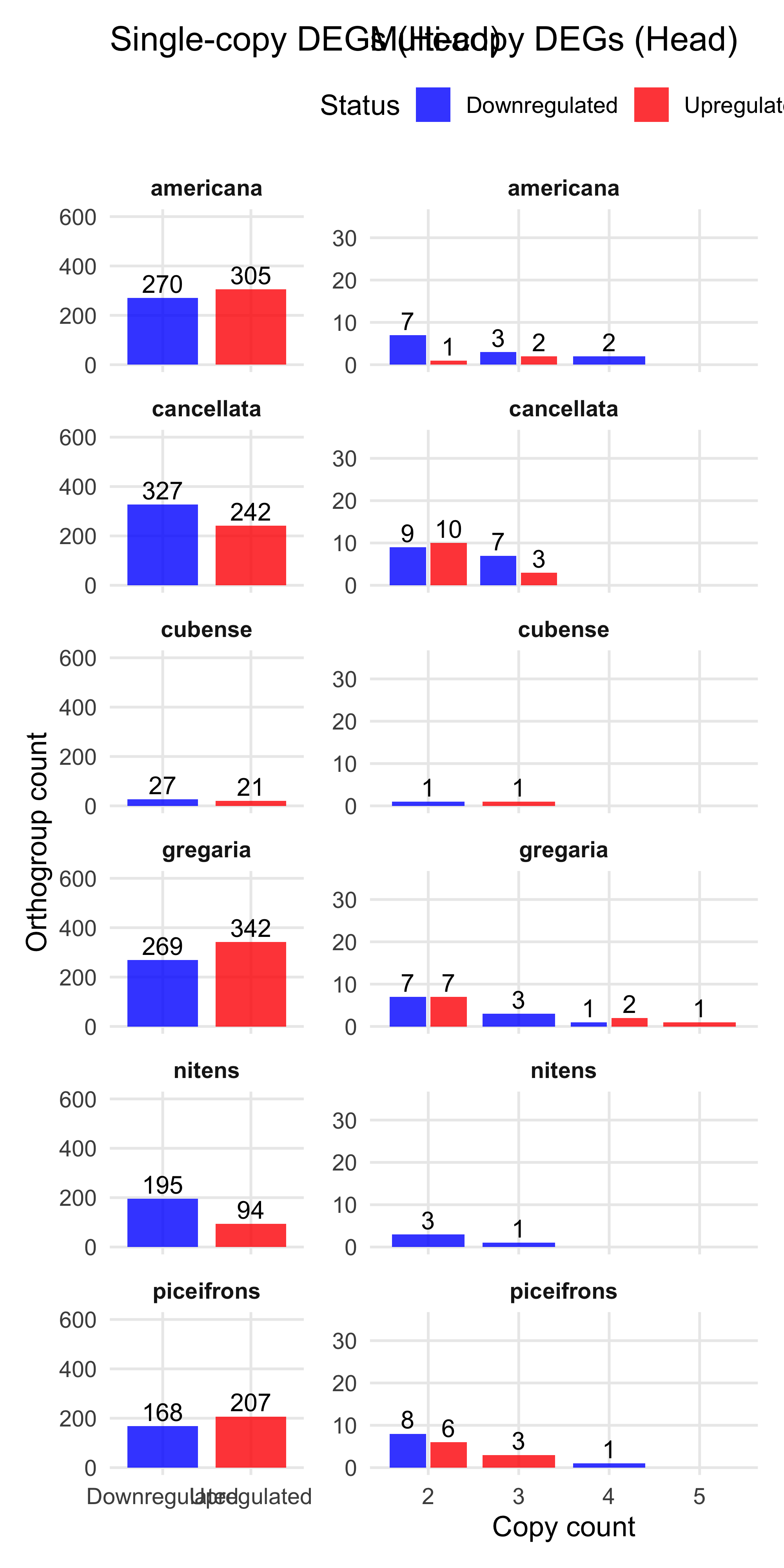
| Version | Author | Date |
|---|---|---|
| a2d2955 | Maeva TECHER | 2025-07-01 |
We found the maximum of copies upregulated genes in one orthogroup is 6 and 9 downregulated. So we decide to make a cap at 5 for plotting.
As a first control, we want to make sure that within an orthogroup, if we have multi-copies of DEG, they would behave the same. If not, and some copies are upregulated while other are downregulated, then we will separate these orthogroups and check them later.
# --- Step 1: Prepare input data ---
summary_df <- summary_table_pivot_Schisto %>%
  filter(Orthogroup != "Unassigned")

species_order <- c("gregaria_Head", "nitens_Head", "cancellata_Head", "piceifrons_Head",
                   "americana_Head", "cubense_Head")

long_df <- summary_df %>%
  pivot_longer(cols = ends_with("_Head"), names_to = "Sample", values_to = "Status") %>%
  filter(Sample %in% species_order)

# Step 1: Filter for Up/Down only
contrast_df <- long_df %>%
  filter(Status %in% c("Upregulated", "Downregulated")) %>%
  group_by(Orthogroup, Sample) %>%
  summarise(
    n_up = sum(Status == "Upregulated"),
    n_down = sum(Status == "Downregulated"),
    .groups = "drop"
  ) %>%
  filter(n_up > 0 & n_down > 0)

# View result: orthogroups with both up and downregulation in the same sample
print(contrast_df)
# A tibble: 11 × 4
Orthogroup Sample n_up n_down
<chr> <chr> <int> <int>
1 OG0000002 piceifrons_Head 1 2
2 OG0000014 piceifrons_Head 1 1
3 OG0000095 piceifrons_Head 1 1
4 OG0000097 cancellata_Head 1 1
5 OG0000154 americana_Head 1 1
6 OG0000154 piceifrons_Head 1 4
7 OG0000160 americana_Head 1 1
8 OG0000163 cancellata_Head 1 1
9 OG0000290 cancellata_Head 1 3
10 OG0000560 gregaria_Head 2 1
11 OG0001343 cancellata_Head 1 1We have 35 groups for which there are contrasting patterns, so we will separate them for the heatmap:
# --- Step 2: Count Up/Down per OG × Sample and classify ---
deg_counts <- long_df %>%
  group_by(Orthogroup, Sample) %>%
  summarize(
    Up = sum(Status == "Upregulated", na.rm = TRUE),
    Down = sum(Status == "Downregulated", na.rm = TRUE),
    .groups = "drop"
  ) %>%
  mutate(
    Category = case_when(
      Up > 0 & Down > 0 ~ "Both",
      Up > 0 & Down == 0 ~ "Up",
      Down > 0 & Up == 0 ~ "Down",
      TRUE ~ "None"
    ),
    Value = case_when(
      Category == "Both" ~ 999,
      Category == "Up" ~ pmin(Up, 5),
      Category == "Down" ~ -pmin(Down, 5),
      TRUE ~ 0
    )
  )

# --- Step 3: Identify contrasting orthogroups ---
contrasting_orthogroups <- deg_counts %>%
  filter(Category == "Both") %>%
  pull(Orthogroup) %>%
  unique()

# --- Step 4: Classify OGs by copy number ---
orthogroup_classification <- deg_counts %>%
  pivot_longer(cols = c(Up, Down), names_to = "Direction", values_to = "Count") %>%
  group_by(Orthogroup) %>%
  summarise(MaxCopy = max(Count), .groups = "drop") %>%
  mutate(Category = if_else(MaxCopy > 1, "Multi", "Single"))

# --- Step 5: Separate Single and Multi (excluding contrasting OGs from Multi) ---
deg_counts_single <- deg_counts %>%
  filter(Orthogroup %in% orthogroup_classification$Orthogroup[
    orthogroup_classification$Category == "Single"])

deg_counts_multi <- deg_counts %>%
  filter(
    Orthogroup %in% orthogroup_classification$Orthogroup[
      orthogroup_classification$Category == "Multi"],
    !Orthogroup %in% contrasting_orthogroups
  )

# --- Step 6: Prepare heatmap matrices ---
mat_single <- deg_counts_single %>%
  select(Orthogroup, Sample, Value) %>%
  pivot_wider(names_from = Orthogroup, values_from = Value, values_fill = 0) %>%
  column_to_rownames("Sample") %>%
  .[species_order, , drop = FALSE] %>%
  .[, colSums(abs(.)) > 0, drop = FALSE]

mat_multi <- deg_counts_multi %>%
  select(Orthogroup, Sample, Value) %>%
  pivot_wider(names_from = Orthogroup, values_from = Value, values_fill = 0) %>%
  column_to_rownames("Sample") %>%
  .[species_order, , drop = FALSE] %>%
  .[, colSums(abs(.)) > 0, drop = FALSE]

mat_contrast <- deg_counts %>%
  filter(Orthogroup %in% contrasting_orthogroups) %>%
  select(Orthogroup, Sample, Value) %>%
  pivot_wider(names_from = Orthogroup, values_from = Value, values_fill = 0) %>%
  column_to_rownames("Sample") %>%
  .[species_order, , drop = FALSE] %>%
  .[, colSums(abs(.)) > 0, drop = FALSE]

# --- Step 7: Define color scale ---
deg_colors <- c(
  "-5" = "#00008B",
  "-4" = "#2133A3",
  "-3" = "#4367BB",
  "-2" = "#659AD3",
  "-1" = "#87CEEB",
   "0" = "white",
   "1" = "#FC9272",
   "2" = "#E36D58",
   "3" = "#CA493F",
   "4" = "#B12426",
   "5" = "#99000D",
  "999" = "purple"
)

col_fun <- circlize::colorRamp2(
  breaks = as.numeric(names(deg_colors)),
  colors = unname(deg_colors)
)

# --- Step 8: Create heatmap objects (not drawn yet) ---
ht_single <- Heatmap(mat_single,
  name = "DEG Count",
  col = col_fun,
  cluster_rows = FALSE,
  cluster_columns = TRUE,
  row_split = factor(rownames(mat_single), levels = species_order),
  row_gap = unit(4, "mm"),
  row_title = "Single-copy DEGs",
  column_title = "Single-copy DEG Orthogroups",
  show_column_names = FALSE,
  row_names_gp = gpar(fontsize = 10)
)


ht_multi <- Heatmap(mat_multi,
  name = "DEG Count",
  col = col_fun,
  cluster_rows = FALSE,
  cluster_columns = TRUE,
  row_split = factor(rownames(mat_multi), levels = species_order),
  row_gap = unit(4, "mm"),
  row_title = "Multi-copy DEGs",
  column_title = "Multi-copy DEG Orthogroups (No Conflict)",
  show_column_names = FALSE,
  row_names_gp = gpar(fontsize = 10)
)


ht_contrast <-Heatmap(mat_contrast,
  name = "DEG Count",
  col = col_fun,
  cluster_rows = FALSE,
  cluster_columns = TRUE,
  row_split = factor(rownames(mat_contrast), levels = species_order),
  row_gap = unit(4, "mm"),
  row_title = "Contrasting DEGs",
  column_title = "Orthogroups with both Up and Down in same species",
  show_column_names = FALSE,
  row_names_gp = gpar(fontsize = 10)
)

# --- Step 9: Custom legends ---
legend_ramp <- Legend(
  col_fun = circlize::colorRamp2(-5:5, deg_colors[as.character(-5:5)]),
  title = "DEG copy number",
  at = -5:5,
  labels = as.character(-5:5),
  legend_height = unit(3, "cm")
)

legend_contrast <- Legend(
  labels = "Both",
  title = "Contrasting",
  legend_gp = gpar(fill = "purple"),
  grid_height = unit(0.3, "cm")
)

leg_combined <- packLegend(legend_ramp, legend_contrast)

# --- Step 10: Draw combined plot with custom legend ---
draw(ht_single, annotation_legend_list = list(legend_ramp))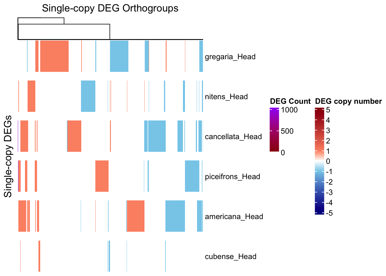
| Version | Author | Date |
|---|---|---|
| a2d2955 | Maeva TECHER | 2025-07-01 |
draw(ht_multi, annotation_legend_list = list(legend_ramp))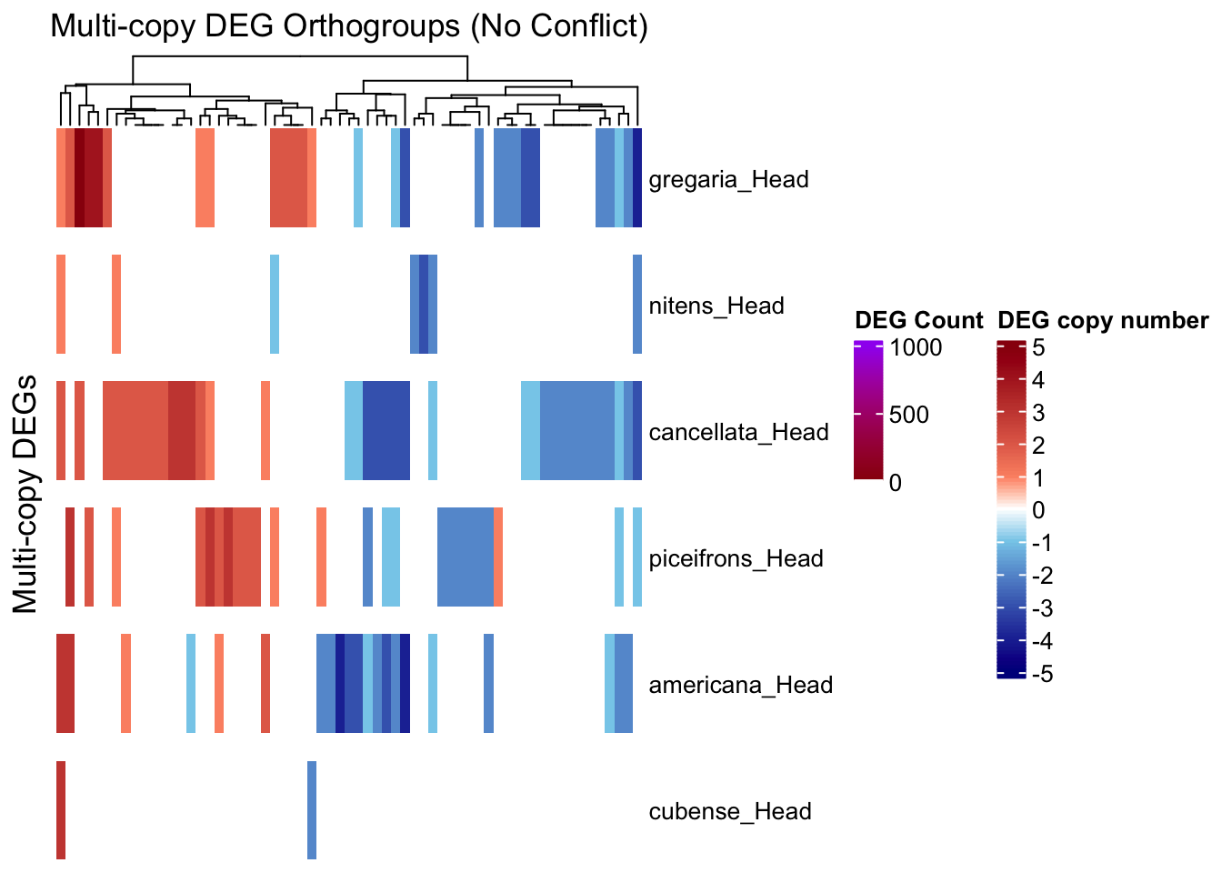
| Version | Author | Date |
|---|---|---|
| a2d2955 | Maeva TECHER | 2025-07-01 |
draw(ht_contrast, annotation_legend_list = list(leg_combined))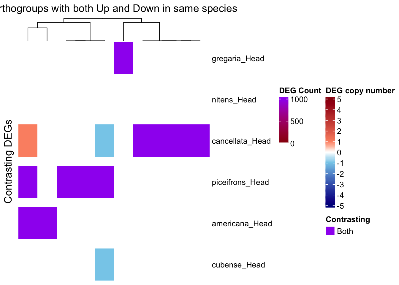
| Version | Author | Date |
|---|---|---|
| a2d2955 | Maeva TECHER | 2025-07-01 |
Thorax-tissue
# === STEP 1: Reshape summary_table_pivot into long format ===
deg_long <- summary_table_pivot_Schisto %>%
  pivot_longer(
    cols = ends_with(c("_Head", "_Thorax")),
    names_to = "Sample",
    values_to = "Status"
  ) %>%
  separate(Sample, into = c("Species", "Tissue"), sep = "_") %>%
  filter(Status %in% c("Upregulated", "Downregulated"))

# === STEP 2: Count DEGs per Orthogroup × Species × Tissue × Status ===
deg_summary_counts <- deg_long %>%
  filter(Orthogroup != "Unassigned") %>%  # Exclude unassigned orthogroups
  group_by(Orthogroup, Orthogroup_Type, Species, Tissue, Status) %>%
  summarise(CopyCount = n(), .groups = "drop") %>%
  mutate(CopyCount = as.integer(CopyCount))

# === STEP 3: Define plotting function ==
plot_deg_distribution_split <- function(tissue_name) {
  # Filter the full plot data
  plot_df <- deg_summary_counts %>%
    filter(Tissue == tissue_name) %>%
    dplyr::count(Species, Status, CopyCount)

  # Panel 1: Single-copy orthogroups
  plot_single <- ggplot(filter(plot_df, CopyCount == 1),
                        aes(x = Status, y = n, fill = Status)) +
    geom_bar(stat = "identity", position = "dodge", width = 0.8, alpha = 0.8) +
    facet_wrap(~Species, ncol = 1) +
    geom_text(aes(label = n), vjust = -0.3, size = 4) +
    labs(
      title = paste("Single-copy DEGs (", tissue_name, ")", sep = ""),
      x = NULL,
      y = "Orthogroup count"
    ) +
    coord_cartesian(ylim = c(0, 600)) +
    scale_fill_manual(values = c("Upregulated" = "red", "Downregulated" = "blue")) +
    theme_minimal(base_size = 13) +
    theme(
      panel.grid.minor = element_blank(),
      legend.position = "none",
      strip.text = element_text(face = "bold")
    )

  # Panel 2: Multi-copy orthogroups, y limited to 40
  plot_multi <- ggplot(filter(plot_df, CopyCount > 1),
                       aes(x = CopyCount, y = n, fill = Status)) +
    geom_bar(stat = "identity", position = position_dodge(0.9), width = 0.8, alpha = 0.8) +
    geom_text(aes(label = ifelse(n < 100, n, "")),
              position = position_dodge(width = 0.9),
              vjust = -0.3, size = 4) +
    facet_wrap(~Species, ncol = 1) +
    labs(
      title = paste("Multi-copy DEGs (", tissue_name, ")", sep = ""),
      x = "Copy count",
      y = NULL
    ) +
    coord_cartesian(ylim = c(0, 35)) +
    scale_x_continuous(breaks = 2:15) +
    scale_fill_manual(values = c("Upregulated" = "red", "Downregulated" = "blue")) +
    theme_minimal(base_size = 13) +
    theme(
      panel.grid.minor  = element_blank(),
      legend.position = "top",
      strip.text = element_text(face = "bold")
    )

  # Combine plots side by side
  plot_single + plot_multi + plot_layout(widths = c(1, 2))
}

plot_deg_distribution_split("Thorax")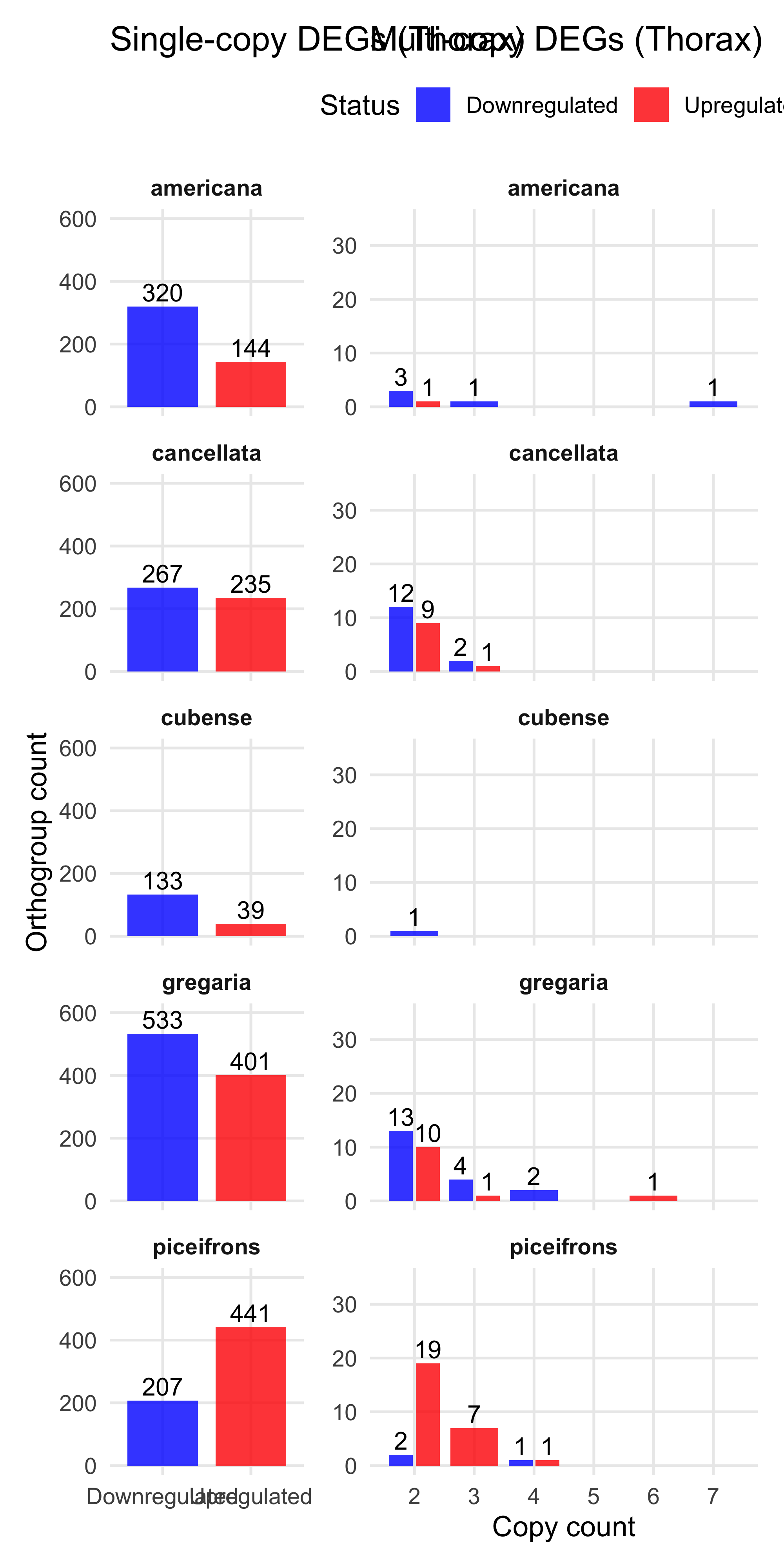
| Version | Author | Date |
|---|---|---|
| a2d2955 | Maeva TECHER | 2025-07-01 |
# --- Step 1: Prepare input data ---
summary_df <- summary_table_pivot_Schisto %>%
  filter(Orthogroup != "Unassigned")

species_order <- c("gregaria_Thorax", "cancellata_Thorax", "piceifrons_Thorax",
                   "americana_Thorax", "cubense_Thorax")

long_df <- summary_df %>%
  pivot_longer(cols = ends_with("_Thorax"), names_to = "Sample", values_to = "Status") %>%
  filter(Sample %in% species_order)

# Step 1: Filter for Up/Down only
contrast_df <- long_df %>%
  filter(Status %in% c("Upregulated", "Downregulated")) %>%
  group_by(Orthogroup, Sample) %>%
  summarise(
    n_up = sum(Status == "Upregulated"),
    n_down = sum(Status == "Downregulated"),
    .groups = "drop"
  ) %>%
  filter(n_up > 0 & n_down > 0)

# View result: orthogroups with both up and downregulation in the same sample
print(contrast_df)
# A tibble: 11 × 4
Orthogroup Sample n_up n_down
<chr> <chr> <int> <int>
1 OG0000002 piceifrons_Thorax 3 1
2 OG0000008 piceifrons_Thorax 1 2
3 OG0000069 piceifrons_Thorax 4 1
4 OG0000076 gregaria_Thorax 1 1
5 OG0000084 piceifrons_Thorax 1 1
6 OG0000097 cancellata_Thorax 1 1
7 OG0000142 americana_Thorax 1 1
8 OG0000163 cancellata_Thorax 1 1
9 OG0000178 gregaria_Thorax 1 1
10 OG0000245 cubense_Thorax 1 2
11 OG0000290 cancellata_Thorax 1 2We have 37 groups for which there are contrasting patterns, so we will separate them for the heatmap:
# --- Step 2: Count Up/Down per OG × Sample and classify ---
deg_counts <- long_df %>%
  group_by(Orthogroup, Sample) %>%
  summarize(
    Up = sum(Status == "Upregulated", na.rm = TRUE),
    Down = sum(Status == "Downregulated", na.rm = TRUE),
    .groups = "drop"
  ) %>%
  mutate(
    Category = case_when(
      Up > 0 & Down > 0 ~ "Both",
      Up > 0 & Down == 0 ~ "Up",
      Down > 0 & Up == 0 ~ "Down",
      TRUE ~ "None"
    ),
    Value = case_when(
      Category == "Both" ~ 999,
      Category == "Up" ~ pmin(Up, 5),
      Category == "Down" ~ -pmin(Down, 5),
      TRUE ~ 0
    )
  )

# --- Step 3: Identify contrasting orthogroups ---
contrasting_orthogroups <- deg_counts %>%
  filter(Category == "Both") %>%
  pull(Orthogroup) %>%
  unique()

# --- Step 4: Classify OGs by copy number ---
orthogroup_classification <- deg_counts %>%
  pivot_longer(cols = c(Up, Down), names_to = "Direction", values_to = "Count") %>%
  group_by(Orthogroup) %>%
  summarise(MaxCopy = max(Count), .groups = "drop") %>%
  mutate(Category = if_else(MaxCopy > 1, "Multi", "Single"))

# --- Step 5: Separate Single and Multi (excluding contrasting OGs from Multi) ---
deg_counts_single <- deg_counts %>%
  filter(Orthogroup %in% orthogroup_classification$Orthogroup[
    orthogroup_classification$Category == "Single"])

deg_counts_multi <- deg_counts %>%
  filter(
    Orthogroup %in% orthogroup_classification$Orthogroup[
      orthogroup_classification$Category == "Multi"],
    !Orthogroup %in% contrasting_orthogroups
  )

# --- Step 6: Prepare heatmap matrices ---
mat_single <- deg_counts_single %>%
  select(Orthogroup, Sample, Value) %>%
  pivot_wider(names_from = Orthogroup, values_from = Value, values_fill = 0) %>%
  column_to_rownames("Sample") %>%
  .[species_order, , drop = FALSE] %>%
  .[, colSums(abs(.)) > 0, drop = FALSE]

mat_multi <- deg_counts_multi %>%
  select(Orthogroup, Sample, Value) %>%
  pivot_wider(names_from = Orthogroup, values_from = Value, values_fill = 0) %>%
  column_to_rownames("Sample") %>%
  .[species_order, , drop = FALSE] %>%
  .[, colSums(abs(.)) > 0, drop = FALSE]

mat_contrast <- deg_counts %>%
  filter(Orthogroup %in% contrasting_orthogroups) %>%
  select(Orthogroup, Sample, Value) %>%
  pivot_wider(names_from = Orthogroup, values_from = Value, values_fill = 0) %>%
  column_to_rownames("Sample") %>%
  .[species_order, , drop = FALSE] %>%
  .[, colSums(abs(.)) > 0, drop = FALSE]

# --- Step 7: Define color scale ---
deg_colors <- c(
  "-5" = "#00008B",
  "-4" = "#2133A3",
  "-3" = "#4367BB",
  "-2" = "#659AD3",
  "-1" = "#87CEEB",
   "0" = "white",
   "1" = "#FC9272",
   "2" = "#E36D58",
   "3" = "#CA493F",
   "4" = "#B12426",
   "5" = "#99000D",
  "999" = "purple"
)

col_fun <- circlize::colorRamp2(
  breaks = as.numeric(names(deg_colors)),
  colors = unname(deg_colors)
)

# --- Step 8: Create heatmap objects (not drawn yet) ---
ht_single <- Heatmap(mat_single,
  name = "DEG Count",
  col = col_fun,
  cluster_rows = FALSE,
  cluster_columns = TRUE,
  row_split = factor(rownames(mat_single), levels = species_order),
  row_gap = unit(4, "mm"),
  row_title = "Single-copy DEGs",
  column_title = "Single-copy DEG Orthogroups",
  show_column_names = FALSE,
  row_names_gp = gpar(fontsize = 10)
)


ht_multi <- Heatmap(mat_multi,
  name = "DEG Count",
  col = col_fun,
  cluster_rows = FALSE,
  cluster_columns = TRUE,
  row_split = factor(rownames(mat_multi), levels = species_order),
  row_gap = unit(4, "mm"),
  row_title = "Multi-copy DEGs",
  column_title = "Multi-copy DEG Orthogroups (No Conflict)",
  show_column_names = FALSE,
  row_names_gp = gpar(fontsize = 10)
)


ht_contrast <-Heatmap(mat_contrast,
  name = "DEG Count",
  col = col_fun,
  cluster_rows = FALSE,
  cluster_columns = TRUE,
  row_split = factor(rownames(mat_contrast), levels = species_order),
  row_gap = unit(4, "mm"),
  row_title = "Contrasting DEGs",
  column_title = "Orthogroups with both Up and Down in same species",
  show_column_names = FALSE,
  row_names_gp = gpar(fontsize = 10)
)

# --- Step 9: Custom legends ---
legend_ramp <- Legend(
  col_fun = circlize::colorRamp2(-5:5, deg_colors[as.character(-5:5)]),
  title = "DEG copy number",
  at = -5:5,
  labels = as.character(-5:5),
  legend_height = unit(3, "cm")
)

legend_contrast <- Legend(
  labels = "Both",
  title = "Contrasting",
  legend_gp = gpar(fill = "purple"),
  grid_height = unit(0.3, "cm")
)

leg_combined <- packLegend(legend_ramp, legend_contrast)

# --- Step 10: Draw combined plot with custom legend ---
draw(ht_single, annotation_legend_list = list(legend_ramp))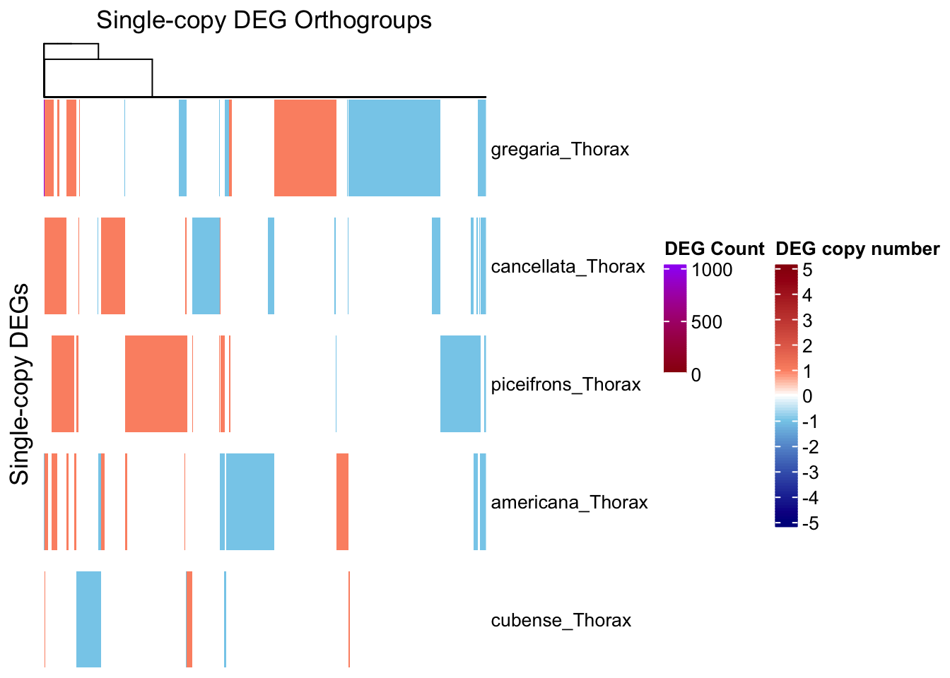
| Version | Author | Date |
|---|---|---|
| a2d2955 | Maeva TECHER | 2025-07-01 |
draw(ht_multi, annotation_legend_list = list(legend_ramp))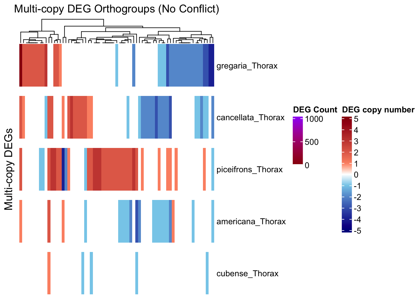
| Version | Author | Date |
|---|---|---|
| a2d2955 | Maeva TECHER | 2025-07-01 |
draw(ht_contrast, annotation_legend_list = list(leg_combined))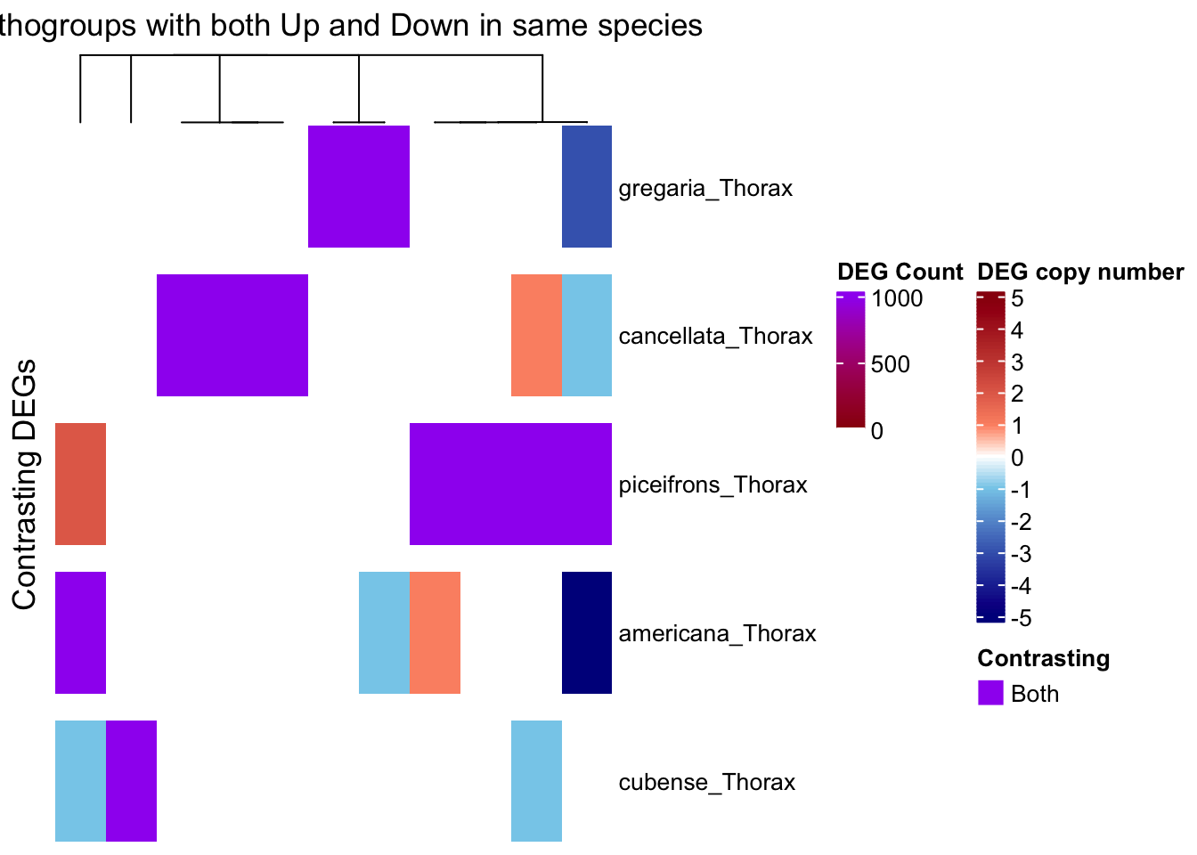
| Version | Author | Date |
|---|---|---|
| a2d2955 | Maeva TECHER | 2025-07-01 |
Polyneoptera-based I2
Head-tissue
First we check what is the maximum number of gene copies within an orthogroup that can be upregulated or downregulated in the same species:
# === STEP 1: Reshape summary_table_pivot into long format ===
deg_long <- summary_table_pivot_Polyneoptera %>%
  pivot_longer(
    cols = ends_with(c("_Head", "_Thorax")),
    names_to = "Sample",
    values_to = "Status"
  ) %>%
  separate(Sample, into = c("Species", "Tissue"), sep = "_") %>%
  filter(Status %in% c("Upregulated", "Downregulated"))

# === STEP 2: Count DEGs per Orthogroup × Species × Tissue × Status ===
deg_summary_counts <- deg_long %>%
  filter(Orthogroup != "Unassigned") %>%  # Exclude unassigned orthogroups
  group_by(Orthogroup, Orthogroup_Type, Species, Tissue, Status) %>%
  summarise(CopyCount = n(), .groups = "drop") %>%
  mutate(CopyCount = as.integer(CopyCount))

species_order <- c("gregaria","cancellata", "piceifrons", "americana", "cubense","nitens")

# === STEP 3: Define plotting function ==
plot_deg_distribution_split <- function(tissue_name) {

    # Filter the full plot data
  plot_df <- deg_summary_counts %>%
    filter(Tissue == tissue_name) %>%
    mutate(Species = factor(Species, levels = species_order)) %>%
    dplyr::count(Species, Status, CopyCount)

  # Panel 1: Single-copy orthogroups
  plot_single <- ggplot(filter(plot_df, CopyCount == 1),
                        aes(x = Status, y = n, fill = Status)) +
    geom_bar(stat = "identity", position = "dodge", width = 0.8) +
    facet_wrap(~Species, ncol = 1) +
    geom_text(aes(label = ifelse(n < 50, n, "")), vjust = -0.3, size = 4)+
    labs(
      title = paste("Single-copy DEGs (", tissue_name, ")", sep = ""),
      x = NULL,
      y = "Number of Orthogroups"
    ) +
    coord_cartesian(ylim = c(0, 600)) +
    scale_fill_manual(values = c("Upregulated" = "red", "Downregulated" = "blue")) +
    theme_minimal(base_size = 13) +
theme(
  panel.grid.major.x = element_blank(),
  panel.grid.minor.x = element_blank(),
  panel.grid.major.y = element_line(),
  panel.grid.minor.y = element_blank(),
  legend.position = "none",
  strip.text = element_text(face = "bold.italic", size = 14),
  axis.text.x = element_text(face = "bold", size = 14, colour = "black")  # <-- added
)


  # Panel 2: Multi-copy orthogroups, y limited to 40
  plot_multi <- ggplot(filter(plot_df, CopyCount > 1),
                       aes(x = CopyCount, y = n, fill = Status)) +
    geom_bar(stat = "identity", position = position_dodge(0.9), width = 0.8) +
    geom_text(aes(label = ifelse(n < 50, n, "")),
          position = position_dodge(width = 0.9),
          vjust = -0.3, size = 4)+
    facet_wrap(~Species, ncol = 1) +
    labs(
      title = paste("Multi-copy DEGs (", tissue_name, ")", sep = ""),
      x = "Number of gene copies",
      y = NULL
    ) +
    coord_cartesian(ylim = c(0, 35)) +
    scale_x_continuous(breaks = 2:9,limits = c(1.5, 9.5))+
    scale_fill_manual(values = c("Upregulated" = "red", "Downregulated" = "blue")) +
    theme_minimal(base_size = 13) +
theme(
  panel.grid.major.x = element_blank(),
  panel.grid.minor.x = element_blank(),
  panel.grid.major.y = element_line(),
  panel.grid.minor.y = element_blank(),
  legend.position = "top",
  strip.text = element_text(face = "bold.italic", size = 14),
  axis.text.x = element_text(face = "bold", size = 14, colour = "black")   # <-- added
)

  # Combine plots side by side
  plot_single + plot_multi + plot_layout(widths = c(1, 2))
}

plot_deg_distribution_split("Head")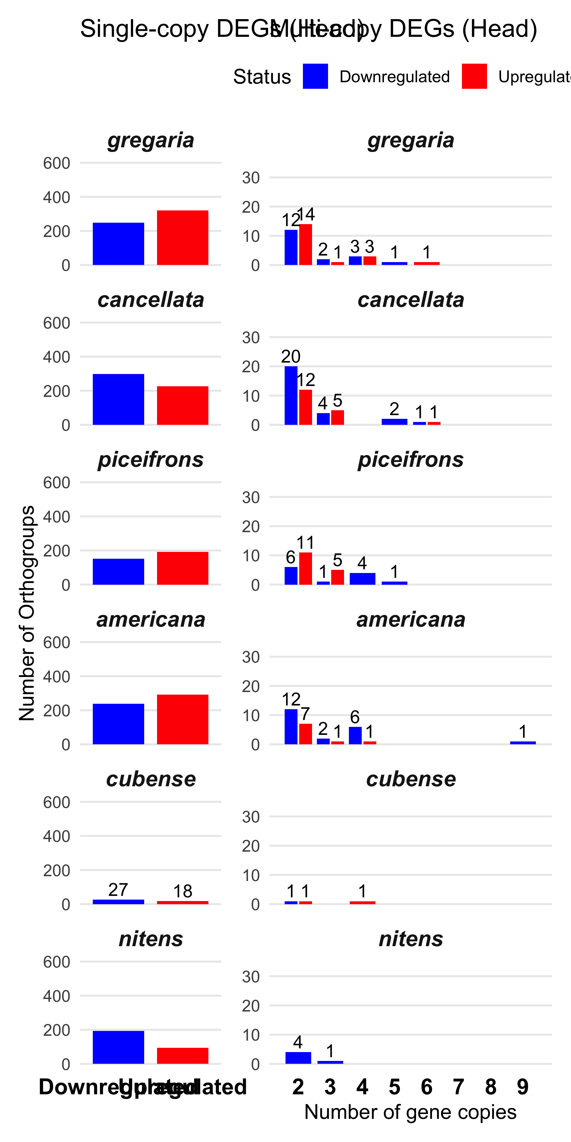
| Version | Author | Date |
|---|---|---|
| a2d2955 | Maeva TECHER | 2025-07-01 |
We found the maximum of copies upregulated genes in one orthogroup is 6 and 9 downregulated. So we decide to make a cap at 5 for plotting.
As a first control, we want to make sure that within an orthogroup, if we have multi-copies of DEG, they would behave the same. If not, and some copies are upregulated while other are downregulated, then we will separate these orthogroups and check them later.
# --- Step 1: Prepare input data ---
summary_df <- summary_table_pivot_Polyneoptera %>%
  filter(Orthogroup != "Unassigned")

species_order <- c("gregaria_Head", "nitens_Head", "cancellata_Head", "piceifrons_Head",
                   "americana_Head", "cubense_Head")

long_df <- summary_df %>%
  pivot_longer(cols = ends_with("_Head"), names_to = "Sample", values_to = "Status") %>%
  filter(Sample %in% species_order)

# Step 1: Filter for Up/Down only
contrast_df <- long_df %>%
  filter(Status %in% c("Upregulated", "Downregulated")) %>%
  group_by(Orthogroup, Sample) %>%
  summarise(
    n_up = sum(Status == "Upregulated"),
    n_down = sum(Status == "Downregulated"),
    .groups = "drop"
  ) %>%
  filter(n_up > 0 & n_down > 0)

# View result: orthogroups with both up and downregulation in the same sample
print(contrast_df)
# A tibble: 35 × 4
Orthogroup Sample n_up n_down
<chr> <chr> <int> <int>
1 OG0000000 americana_Head 1 4
2 OG0000000 piceifrons_Head 1 1
3 OG0000013 cancellata_Head 2 1
4 OG0000014 americana_Head 1 1
5 OG0000014 cancellata_Head 2 1
6 OG0000014 gregaria_Head 6 2
7 OG0000015 gregaria_Head 2 1
8 OG0000019 piceifrons_Head 1 3
9 OG0000035 gregaria_Head 2 1
10 OG0000048 cancellata_Head 1 1
# ℹ 25 more rowsWe have 35 groups for which there are contrasting patterns, so we will separate them for the heatmap:
# --- Step 2: Count Up/Down per OG × Sample and classify ---
deg_counts <- long_df %>%
  group_by(Orthogroup, Orthogroup_Type, Sample) %>%
  summarize(
    Up = sum(Status == "Upregulated", na.rm = TRUE),
    Down = sum(Status == "Downregulated", na.rm = TRUE),
    .groups = "drop"
  ) %>%
  mutate(
    Category = case_when(
      Up > 0 & Down > 0 ~ "Both",
      Up > 0 & Down == 0 ~ "Up",
      Down > 0 & Up == 0 ~ "Down",
      TRUE ~ "None"
    ),
    Value = case_when(
      Category == "Both" ~ 999,
      Category == "Up" ~ pmin(Up, 5),
      Category == "Down" ~ -pmin(Down, 5),
      TRUE ~ 0
    )
  )

# --- Step 3: Identify contrasting orthogroups ---
contrasting_orthogroups <- deg_counts %>%
  filter(Category == "Both") %>%
  pull(Orthogroup) %>%
  unique()

# --- Step 4: Classify OGs by copy number ---
#orthogroup_classification <- deg_counts %>%
#  pivot_longer(cols = c(Up, Down), names_to = "Direction", values_to = "Count") %>%
#  group_by(Orthogroup) %>%
#  summarise(MaxCopy = max(Count), .groups = "drop") %>%
#  mutate(Category = if_else(MaxCopy > 1, "Multi", "Single"))

# --- Step 5: Re-encode Single-copy OGs to strict -1/0/1 only ---
#deg_counts_single <- deg_counts %>%
#  filter(Orthogroup %in% orthogroup_classification$Orthogroup[
#    orthogroup_classification$Category == "Single"]) %>%
#  mutate(
#    Value = case_when(
#      Up > 0 & Down == 0 ~ 1,
#      Down > 0 & Up == 0 ~ -1,
#      TRUE ~ 0  # Includes 'Both' and 'None'
#    )
#  )

#deg_counts_multi <- deg_counts %>%
#  filter(
#    Orthogroup %in% orthogroup_classification$Orthogroup[
#      orthogroup_classification$Category == "Multi"],
#    !Orthogroup %in% contrasting_orthogroups
#  )

# --- Step 4: Classify Single, Multi, and Contrasting OGs using Orthogroup_Type ---
single_OGs <- deg_counts %>% filter(Orthogroup_Type == "SingleCopy")
multi_OGs  <- deg_counts %>%
  filter(Orthogroup_Type == "MultiCopy" & !Orthogroup %in% contrasting_orthogroups)
contrast_OGs <- deg_counts %>% filter(Orthogroup %in% contrasting_orthogroups)

# --- Step 5: Re-encode Single-copy OGs to strict -1/0/1 only ---
deg_counts_single <- single_OGs %>%
  mutate(Value = case_when(
    Up > 0 & Down == 0 ~ 1,
    Down > 0 & Up == 0 ~ -1,
    TRUE ~ 0  # includes Both and None
  ))

deg_counts_multi <- multi_OGs
deg_counts_contrast <- contrast_OGs

# --- Step 6: Prepare heatmap matrices ---
mat_single <- deg_counts_single %>%
  select(Orthogroup, Sample, Value) %>%
  pivot_wider(names_from = Orthogroup, values_from = Value, values_fill = 0) %>%
  column_to_rownames("Sample") %>%
  .[species_order, , drop = FALSE] %>%
  .[, colSums(abs(.)) > 0, drop = FALSE]
# To make sure we have only -1 and 1 values
#unique(as.vector(mat_single))

mat_multi <- deg_counts_multi %>%
  select(Orthogroup, Sample, Value) %>%
  pivot_wider(names_from = Orthogroup, values_from = Value, values_fill = 0) %>%
  column_to_rownames("Sample") %>%
  .[species_order, , drop = FALSE] %>%
  .[, colSums(abs(.)) > 0, drop = FALSE]

mat_contrast <- deg_counts_contrast %>%
  select(Orthogroup, Sample, Value) %>%
  pivot_wider(names_from = Orthogroup, values_from = Value, values_fill = 0) %>%
  column_to_rownames("Sample") %>%
  .[species_order, , drop = FALSE] %>%
  .[, colSums(abs(.)) > 0, drop = FALSE]

# --- Step 7: Define color scale ---
deg_colors <- c(
  "-5" = "#00008B", "-4" = "#2133A3", "-3" = "#4367BB", "-2" = "#659AD3", "-1" = "#87CEEB",
   "0" = "white",
   "1" = "#FC9272", "2" = "#E36D58", "3" = "#CA493F", "4" = "#B12426", "5" = "#99000D",
 "999" = "purple"
)

col_fun <- circlize::colorRamp2(
  breaks = as.numeric(names(deg_colors)),
  colors = unname(deg_colors)
)

col_fun_single <- structure(
  c("#87CEEB", "white", "#FC9272"),
  names = c("-1", "0", "1")
)


# --- Step X: Define clade colors and mapping ---
clade_levels <- c("Polyneoptera", "Orthoptera", "Caelifera", "Schistocerca", "Species_specific")

clade_colors <- c(
  "Polyneoptera"     = "#FFF24C",
  "Orthoptera"       = "#FFBC2F",
  "Caelifera"        = "#12B759",
  "Schistocerca"     = "#72BFFF",
  "Species_specific" = "#854800"
)

get_clade_annotation <- function(matrix_columns) {
  orthogroup_clades <- gene_counts_clade %>%
    select(Orthogroup, Assigned_Clade) %>%
    filter(Orthogroup %in% matrix_columns) %>%
    distinct()
  clade_vector <- setNames(orthogroup_clades$Assigned_Clade, orthogroup_clades$Orthogroup)
  clade_vector[matrix_columns]
}

# --- Step 8: Function for ordered heatmap creation ---
create_clade_split_heatmap <- function(mat, clade_vector, row_title, col_title, col_fun_input) {
  clade_factor <- factor(clade_vector, levels = clade_levels, ordered = TRUE)

  Heatmap(
    mat,
    name = "DEG Count",
    col = col_fun_input,  # Use the passed color function
    cluster_rows = FALSE,
    cluster_columns = TRUE,
    column_split = clade_factor,
    column_title = col_title,
    row_split = factor(rownames(mat), levels = species_order),
    row_gap = unit(4, "mm"),
    top_annotation = HeatmapAnnotation(
      Clade = clade_factor,
      col = list(Clade = clade_colors),
      show_annotation_name = TRUE,
      annotation_name_side = "left"
    ),
    cluster_column_slices = FALSE,
    row_title = row_title,
    show_column_names = FALSE,
    row_names_gp = gpar(fontsize = 10)
  )
}

# --- Step 9: Generate heatmaps using unified function ---
ht_single <- create_clade_split_heatmap(mat_single, get_clade_annotation(colnames(mat_single)),
                                         "Single-copy DEGs (Head)", "Faceted by lineage clade", col_fun_single)
ht_multi <- create_clade_split_heatmap(mat_multi, get_clade_annotation(colnames(mat_multi)),
                                        "Multi-copy DEGs (Head)", "Faceted by lineage clade", col_fun)
ht_contrast <- create_clade_split_heatmap(mat_contrast, get_clade_annotation(colnames(mat_contrast)),
                                           "Contrasting DEGs (Head)", "Faceted by lineage clade", col_fun)

# --- Step 10: Custom legends ---
legend_ramp <- Legend(
  col_fun = circlize::colorRamp2(-5:5, deg_colors[as.character(-5:5)]),
  title = "DEG copy number",
  at = -5:5,
  labels = as.character(-5:5),
  legend_height = unit(3, "cm")
)

legend_contrast <- Legend(
  labels = "Both",
  title = "Contrasting",
  legend_gp = gpar(fill = "purple"),
  grid_height = unit(0.3, "cm")
)

leg_combined <- packLegend(legend_ramp, legend_contrast)

legend_single <- Legend(
  at = c(-1, 0, 1),
  labels = c("Down", "None", "Up"),
  title = "Single-copy DEG",
  legend_gp = gpar(fill = c("#87CEEB", "white", "#FC9272")),
  grid_height = unit(0.4, "cm")
)

# --- Step 11: Draw combined plots ---
draw(ht_single, annotation_legend_list = list(legend_single))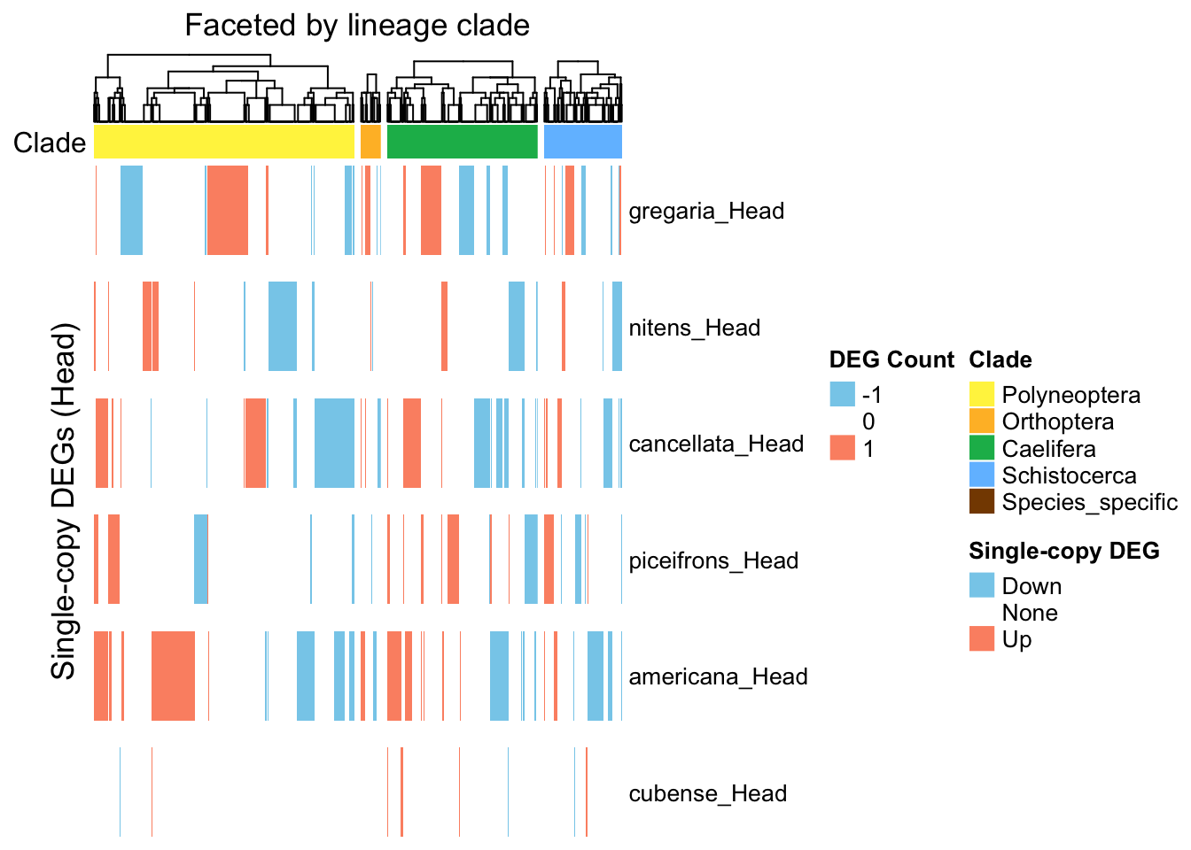
| Version | Author | Date |
|---|---|---|
| a2d2955 | Maeva TECHER | 2025-07-01 |
draw(ht_multi, annotation_legend_list = list(legend_ramp))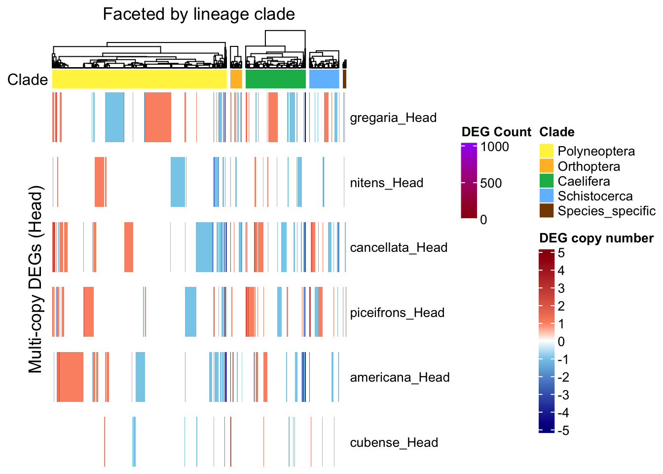
| Version | Author | Date |
|---|---|---|
| a2d2955 | Maeva TECHER | 2025-07-01 |
draw(ht_contrast, annotation_legend_list = list(leg_combined))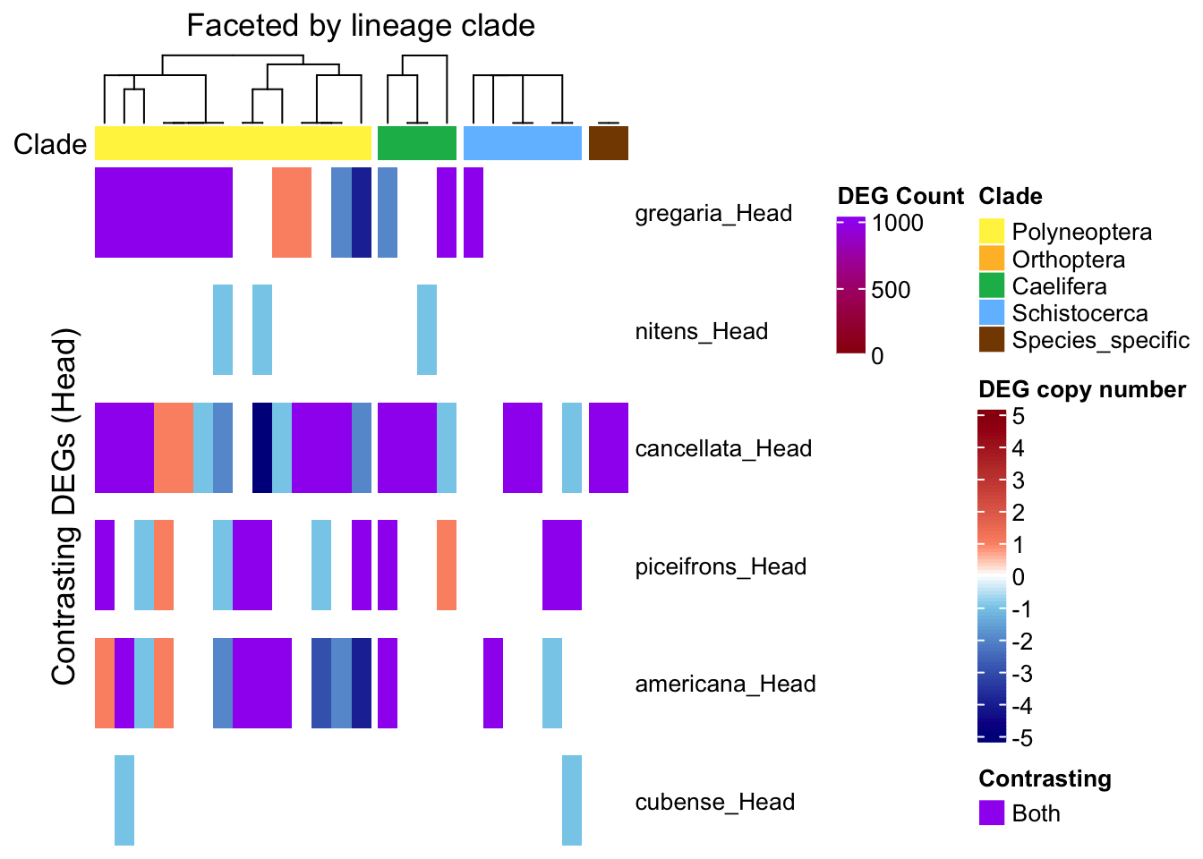
| Version | Author | Date |
|---|---|---|
| a2d2955 | Maeva TECHER | 2025-07-01 |
Thorax-tissue
First we check what is the maximum of copy per one orthogroup that can be upregulated or downregulated in a same species:
# === STEP 1: Reshape summary_table_pivot into long format ===
deg_long <- summary_table_pivot_Polyneoptera %>%
  pivot_longer(
    cols = ends_with(c("_Head", "_Thorax")),
    names_to = "Sample",
    values_to = "Status"
  ) %>%
  separate(Sample, into = c("Species", "Tissue"), sep = "_") %>%
  filter(Status %in% c("Upregulated", "Downregulated"))

# === STEP 2: Count DEGs per Orthogroup × Species × Tissue × Status ===
deg_summary_counts <- deg_long %>%
  filter(Orthogroup != "Unassigned") %>%  # Exclude unassigned orthogroups
  group_by(Orthogroup, Orthogroup_Type, Species, Tissue, Status) %>%
  summarise(CopyCount = n(), .groups = "drop") %>%
  mutate(CopyCount = as.integer(CopyCount))

species_order <- c("gregaria","cancellata", "piceifrons", "americana", "cubense","nitens")

# === STEP 3: Define plotting function ==
plot_deg_distribution_split <- function(tissue_name) {

    # Filter the full plot data
  plot_df <- deg_summary_counts %>%
    filter(Tissue == tissue_name) %>%
    mutate(Species = factor(Species, levels = species_order)) %>%
    dplyr::count(Species, Status, CopyCount)

  # Panel 1: Single-copy orthogroups
  plot_single <- ggplot(filter(plot_df, CopyCount == 1),
                        aes(x = Status, y = n, fill = Status)) +
    geom_bar(stat = "identity", position = "dodge", width = 0.8) +
    facet_wrap(~Species, ncol = 1) +
    geom_text(aes(label = ifelse(n < 50, n, "")), vjust = -0.3, size = 4)+
    labs(
      title = paste("Single-copy DEGs (", tissue_name, ")", sep = ""),
      x = NULL,
      y = "Number of Orthogroups"
    ) +
    coord_cartesian(ylim = c(0, 600)) +
    scale_fill_manual(values = c("Upregulated" = "red", "Downregulated" = "blue")) +
    theme_minimal(base_size = 13) +
theme(
  panel.grid.major.x = element_blank(),
  panel.grid.minor.x = element_blank(),
  panel.grid.major.y = element_line(),
  panel.grid.minor.y = element_blank(),
  legend.position = "none",
  strip.text = element_text(face = "bold.italic", size = 14),
  axis.text.x = element_text(face = "bold", size = 14, colour = "black")  # <-- added
)


  # Panel 2: Multi-copy orthogroups, y limited to 40
  plot_multi <- ggplot(filter(plot_df, CopyCount > 1),
                       aes(x = CopyCount, y = n, fill = Status)) +
    geom_bar(stat = "identity", position = position_dodge(0.9), width = 0.8) +
    geom_text(aes(label = ifelse(n < 50, n, "")),
          position = position_dodge(width = 0.9),
          vjust = -0.3, size = 4)+
    facet_wrap(~Species, ncol = 1) +
    labs(
      title = paste("Multi-copy DEGs (", tissue_name, ")", sep = ""),
      x = "Number of gene copies",
      y = NULL
    ) +
    coord_cartesian(ylim = c(0, 35)) +
    scale_x_continuous(breaks = 2:9,limits = c(1.5, 9.5))+
    scale_fill_manual(values = c("Upregulated" = "red", "Downregulated" = "blue")) +
    theme_minimal(base_size = 13) +
theme(
  panel.grid.major.x = element_blank(),
  panel.grid.minor.x = element_blank(),
  panel.grid.major.y = element_line(),
  panel.grid.minor.y = element_blank(),
  legend.position = "top",
  strip.text = element_text(face = "bold.italic", size = 14),
  axis.text.x = element_text(face = "bold", size = 14, colour = "black")   # <-- added
)

  # Combine plots side by side
  plot_single + plot_multi + plot_layout(widths = c(1, 2))
}

plot_deg_distribution_split("Thorax")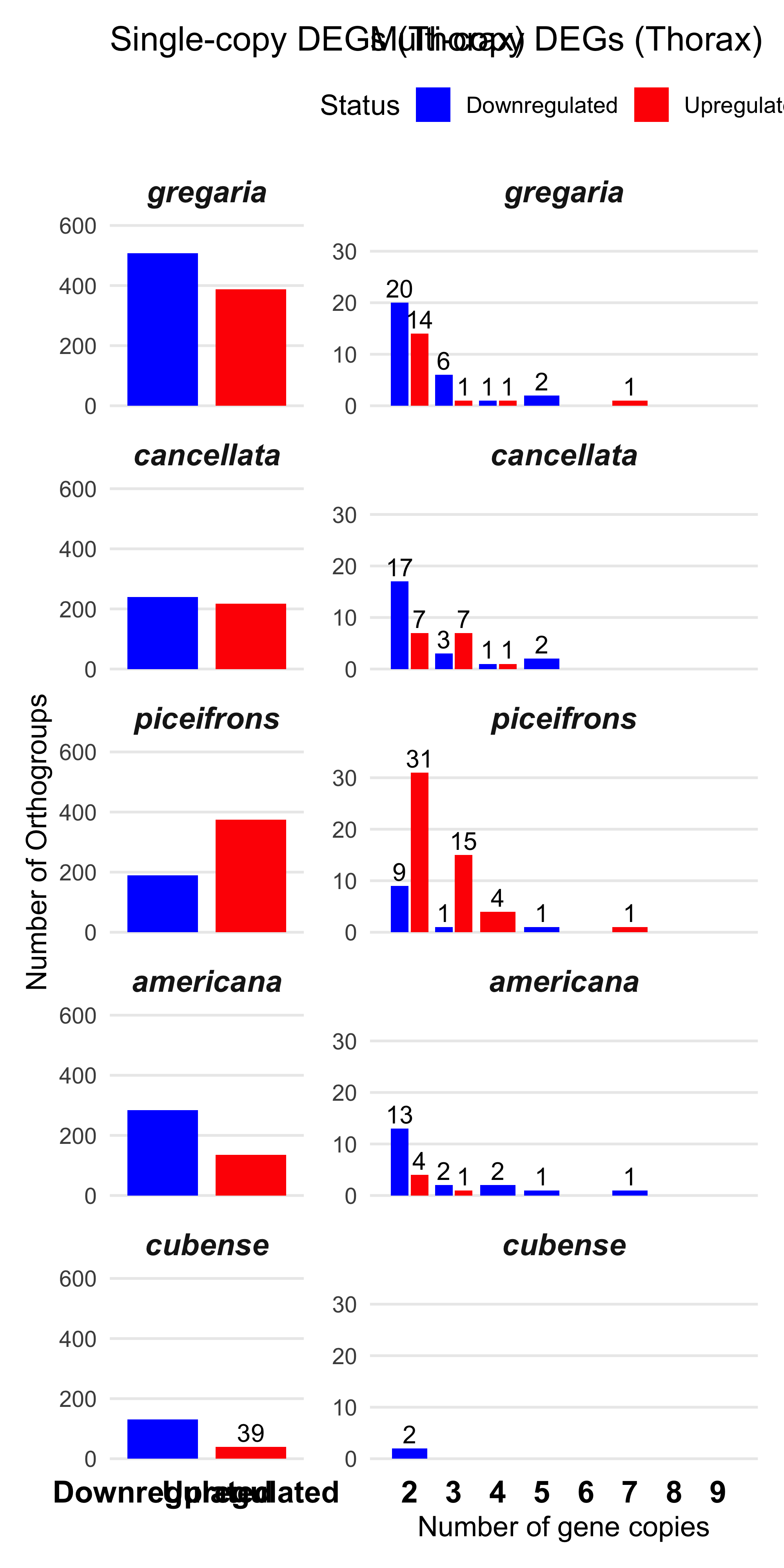
| Version | Author | Date |
|---|---|---|
| a2d2955 | Maeva TECHER | 2025-07-01 |
We found the maximum of copies upregulated genes in one orthogroup is 6 and 9 downregulated. So we decide to make a cap at 5 for plotting.
As a first control, we want to make sure that within an orthogroup, if we have multi-copies of DEG, they would behave the same. If not, and some copies are upregulated while other are downregulated, then we will separate these orthogroups and check them later.
# --- Step 1: Prepare input data ---
summary_df <- summary_table_pivot_Polyneoptera %>%
  filter(Orthogroup != "Unassigned")

species_order <- c("gregaria_Thorax", "cancellata_Thorax", "piceifrons_Thorax",
                   "americana_Thorax", "cubense_Thorax")

long_df <- summary_df %>%
  pivot_longer(cols = ends_with("_Thorax"), names_to = "Sample", values_to = "Status") %>%
  filter(Sample %in% species_order)

# Step 1: Filter for Up/Down only
contrast_df <- long_df %>%
  filter(Status %in% c("Upregulated", "Downregulated")) %>%
  group_by(Orthogroup, Sample) %>%
  summarise(
    n_up = sum(Status == "Upregulated"),
    n_down = sum(Status == "Downregulated"),
    .groups = "drop"
  ) %>%
  filter(n_up > 0 & n_down > 0)

# View result: orthogroups with both up and downregulation in the same sample
print(contrast_df)
# A tibble: 37 × 4
Orthogroup Sample n_up n_down
<chr> <chr> <int> <int>
1 OG0000000 cancellata_Thorax 3 5
2 OG0000001 gregaria_Thorax 4 1
3 OG0000003 cancellata_Thorax 3 1
4 OG0000003 piceifrons_Thorax 1 2
5 OG0000013 cancellata_Thorax 3 1
6 OG0000013 piceifrons_Thorax 2 2
7 OG0000014 americana_Thorax 2 2
8 OG0000014 cancellata_Thorax 3 3
9 OG0000014 gregaria_Thorax 7 2
10 OG0000014 piceifrons_Thorax 7 1
# ℹ 27 more rowsWe have 37 groups for which there are contrasting patterns, so we will separate them for the heatmap:
# --- Step 2: Count Up/Down per OG × Sample and classify ---
deg_counts <- long_df %>%
  group_by(Orthogroup, Orthogroup_Type, Sample) %>%
  summarize(
    Up = sum(Status == "Upregulated", na.rm = TRUE),
    Down = sum(Status == "Downregulated", na.rm = TRUE),
    .groups = "drop"
  ) %>%
  mutate(
    Category = case_when(
      Up > 0 & Down > 0 ~ "Both",
      Up > 0 & Down == 0 ~ "Up",
      Down > 0 & Up == 0 ~ "Down",
      TRUE ~ "None"
    ),
    Value = case_when(
      Category == "Both" ~ 999,
      Category == "Up" ~ pmin(Up, 5),
      Category == "Down" ~ -pmin(Down, 5),
      TRUE ~ 0
    )
  )

# --- Step 3: Identify contrasting orthogroups ---
contrasting_orthogroups <- deg_counts %>%
  filter(Category == "Both") %>%
  pull(Orthogroup) %>%
  unique()

# --- Step 4: Classify OGs by copy number ---
#orthogroup_classification <- deg_counts %>%
#  pivot_longer(cols = c(Up, Down), names_to = "Direction", values_to = "Count") %>%
#  group_by(Orthogroup) %>%
#  summarise(MaxCopy = max(Count), .groups = "drop") %>%
#  mutate(Category = if_else(MaxCopy > 1, "Multi", "Single"))

# --- Step 5: Re-encode Single-copy OGs to strict -1/0/1 only ---
#deg_counts_single <- deg_counts %>%
#  filter(Orthogroup %in% orthogroup_classification$Orthogroup[
#    orthogroup_classification$Category == "Single"]) %>%
#  mutate(
#    Value = case_when(
#      Up > 0 & Down == 0 ~ 1,
#      Down > 0 & Up == 0 ~ -1,
#      TRUE ~ 0  # Includes 'Both' and 'None'
#    )
#  )

#deg_counts_multi <- deg_counts %>%
#  filter(
#    Orthogroup %in% orthogroup_classification$Orthogroup[
#      orthogroup_classification$Category == "Multi"],
#    !Orthogroup %in% contrasting_orthogroups
#  )

# --- Step 4: Classify Single, Multi, and Contrasting OGs using Orthogroup_Type ---
single_OGs <- deg_counts %>% filter(Orthogroup_Type == "SingleCopy")
multi_OGs  <- deg_counts %>%
  filter(Orthogroup_Type == "MultiCopy" & !Orthogroup %in% contrasting_orthogroups)
contrast_OGs <- deg_counts %>% filter(Orthogroup %in% contrasting_orthogroups)

# --- Step 5: Re-encode Single-copy OGs to strict -1/0/1 only ---
deg_counts_single <- single_OGs %>%
  mutate(Value = case_when(
    Up > 0 & Down == 0 ~ 1,
    Down > 0 & Up == 0 ~ -1,
    TRUE ~ 0  # includes Both and None
  ))

deg_counts_multi <- multi_OGs
deg_counts_contrast <- contrast_OGs

# --- Step 6: Prepare heatmap matrices ---
mat_single <- deg_counts_single %>%
  select(Orthogroup, Sample, Value) %>%
  pivot_wider(names_from = Orthogroup, values_from = Value, values_fill = 0) %>%
  column_to_rownames("Sample") %>%
  .[species_order, , drop = FALSE] %>%
  .[, colSums(abs(.)) > 0, drop = FALSE]
# To make sure we have only -1 and 1 values
#unique(as.vector(mat_single))

mat_multi <- deg_counts_multi %>%
  select(Orthogroup, Sample, Value) %>%
  pivot_wider(names_from = Orthogroup, values_from = Value, values_fill = 0) %>%
  column_to_rownames("Sample") %>%
  .[species_order, , drop = FALSE] %>%
  .[, colSums(abs(.)) > 0, drop = FALSE]

mat_contrast <- deg_counts_contrast %>%
  select(Orthogroup, Sample, Value) %>%
  pivot_wider(names_from = Orthogroup, values_from = Value, values_fill = 0) %>%
  column_to_rownames("Sample") %>%
  .[species_order, , drop = FALSE] %>%
  .[, colSums(abs(.)) > 0, drop = FALSE]

# --- Step 7: Define color scale ---
deg_colors <- c(
  "-5" = "#00008B", "-4" = "#2133A3", "-3" = "#4367BB", "-2" = "#659AD3", "-1" = "#87CEEB",
   "0" = "white",
   "1" = "#FC9272", "2" = "#E36D58", "3" = "#CA493F", "4" = "#B12426", "5" = "#99000D",
 "999" = "purple"
)

col_fun <- circlize::colorRamp2(
  breaks = as.numeric(names(deg_colors)),
  colors = unname(deg_colors)
)

col_fun_single <- structure(
  c("#87CEEB", "white", "#FC9272"),
  names = c("-1", "0", "1")
)


# --- Step X: Define clade colors and mapping ---
clade_levels <- c("Polyneoptera", "Orthoptera", "Caelifera", "Schistocerca", "Species_specific")

clade_colors <- c(
  "Polyneoptera"     = "#FFF24C",
  "Orthoptera"       = "#FFBC2F",
  "Caelifera"        = "#12B759",
  "Schistocerca"     = "#72BFFF",
  "Species_specific" = "#854800"
)

get_clade_annotation <- function(matrix_columns) {
  orthogroup_clades <- gene_counts_clade %>%
    select(Orthogroup, Assigned_Clade) %>%
    filter(Orthogroup %in% matrix_columns) %>%
    distinct()
  clade_vector <- setNames(orthogroup_clades$Assigned_Clade, orthogroup_clades$Orthogroup)
  clade_vector[matrix_columns]
}

# --- Step 8: Function for ordered heatmap creation ---
create_clade_split_heatmap <- function(mat, clade_vector, row_title, col_title, col_fun_input) {
  clade_factor <- factor(clade_vector, levels = clade_levels, ordered = TRUE)

  Heatmap(
    mat,
    name = "DEG Count",
    col = col_fun_input,  # Use the passed color function
    cluster_rows = FALSE,
    cluster_columns = TRUE,
    column_split = clade_factor,
    column_title = col_title,
    row_split = factor(rownames(mat), levels = species_order),
    row_gap = unit(4, "mm"),
    top_annotation = HeatmapAnnotation(
      Clade = clade_factor,
      col = list(Clade = clade_colors),
      show_annotation_name = TRUE,
      annotation_name_side = "left"
    ),
    cluster_column_slices = FALSE,
    row_title = row_title,
    show_column_names = FALSE,
    row_names_gp = gpar(fontsize = 10)
  )
}

# --- Step 9: Generate heatmaps using unified function ---
ht_single <- create_clade_split_heatmap(mat_single, get_clade_annotation(colnames(mat_single)),
                                         "Single-copy DEGs (Thorax)", "Faceted by lineage clade", col_fun_single)
ht_multi <- create_clade_split_heatmap(mat_multi, get_clade_annotation(colnames(mat_multi)),
                                        "Multi-copy DEGs (Thorax)", "Faceted by lineage clade", col_fun)
ht_contrast <- create_clade_split_heatmap(mat_contrast, get_clade_annotation(colnames(mat_contrast)),
                                           "Contrasting DEGs (Thorax)", "Faceted by lineage clade", col_fun)

# --- Step 10: Custom legends ---
legend_ramp <- Legend(
  col_fun = circlize::colorRamp2(-5:5, deg_colors[as.character(-5:5)]),
  title = "DEG copy number",
  at = -5:5,
  labels = as.character(-5:5),
  legend_height = unit(3, "cm")
)

legend_contrast <- Legend(
  labels = "Both",
  title = "Contrasting",
  legend_gp = gpar(fill = "purple"),
  grid_height = unit(0.3, "cm")
)

leg_combined <- packLegend(legend_ramp, legend_contrast)

legend_single <- Legend(
  at = c(-1, 0, 1),
  labels = c("Down", "None", "Up"),
  title = "Single-copy DEG",
  legend_gp = gpar(fill = c("#87CEEB", "white", "#FC9272")),
  grid_height = unit(0.4, "cm")
)

# --- Step 11: Draw combined plots ---
draw(ht_single, annotation_legend_list = list(legend_single))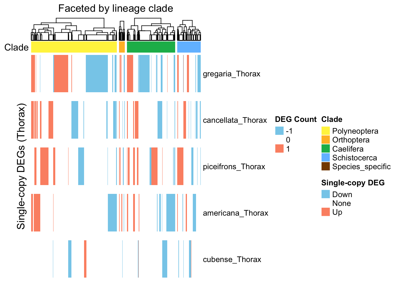
| Version | Author | Date |
|---|---|---|
| a2d2955 | Maeva TECHER | 2025-07-01 |
draw(ht_multi, annotation_legend_list = list(legend_ramp))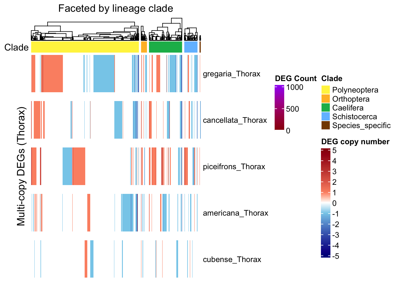
| Version | Author | Date |
|---|---|---|
| a2d2955 | Maeva TECHER | 2025-07-01 |
draw(ht_contrast, annotation_legend_list = list(leg_combined))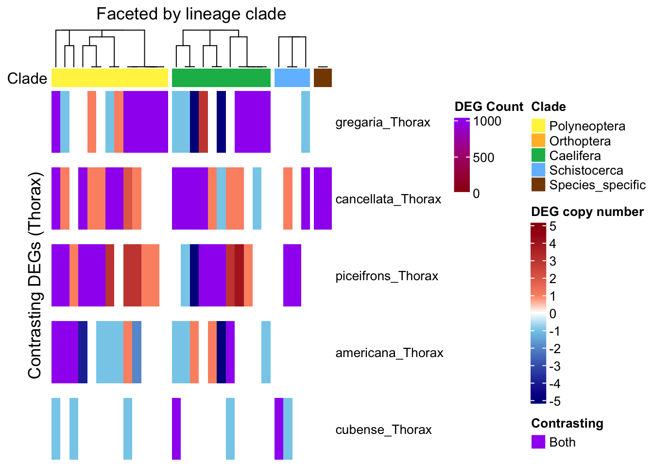
| Version | Author | Date |
|---|---|---|
| a2d2955 | Maeva TECHER | 2025-07-01 |
Combined
# === STEP 1: Reshape summary_table_pivot into long format ===
summary_df <- summary_table_pivot_Polyneoptera %>%
  filter(Orthogroup != "Unassigned")

species_order <- c(
  "gregaria_Head", "gregaria_Thorax", "cancellata_Head", "cancellata_Thorax",
  "piceifrons_Head", "piceifrons_Thorax", "americana_Head", "americana_Thorax",
  "cubense_Head", "cubense_Thorax", "nitens_Head"
)

# Convert wide table to long format
long_df <- summary_df %>%
  pivot_longer(
    cols = ends_with("_Head") | ends_with("_Thorax"),
    names_to = "Sample", values_to = "Status"
  ) %>%
  filter(Sample %in% species_order) %>%
  as_tibble()


# === STEP 2: Define dominant Orthogroup_Type per OG ===
orthogroup_type_map <- long_df %>%
  filter(!is.na(Orthogroup_Type)) %>%
  dplyr::count(Orthogroup, Orthogroup_Type) %>%
  group_by(Orthogroup) %>%
  slice_max(order_by = n, n = 1, with_ties = FALSE) %>%
  ungroup()

# === STEP 3: Count DEGs per Orthogroup × Sample ===
deg_counts <- long_df %>%
  filter(Status %in% c("Upregulated", "Downregulated")) %>%
  group_by(Orthogroup, Sample) %>%
  summarise(
    Up = sum(Status == "Upregulated"),
    Down = sum(Status == "Downregulated"),
    .groups = "drop"
  ) %>%
  mutate(
    Category = case_when(
      Up > 0 & Down > 0 ~ "Both",
      Up > 0 ~ "Up",
      Down > 0 ~ "Down",
      TRUE ~ "None"
    ),
    Value = case_when(
      Category == "Both" ~ 999,
      Category == "Up" ~ pmin(Up, 5),
      Category == "Down" ~ -pmin(Down, 5),
      TRUE ~ 0
    )
  ) %>%
  # Join the cleaned Orthogroup_Type info
  left_join(orthogroup_type_map, by = "Orthogroup")


# Subset to Single-copy only
deg_counts_single <- deg_counts %>%
  filter(Orthogroup_Type == "SingleCopy") %>%
  filter(Value != 999) %>%  # remove contrasting
  mutate(Value = case_when(
    Up > 0 ~ 1,
    Down > 0 ~ -1,
    TRUE ~ 0
  ))

# MULTI-copy: keep only Value ≠ 999
deg_counts_multi <- deg_counts %>%
  filter(
    Orthogroup %in% orthogroup_classification$Orthogroup[
      orthogroup_classification$Category == "Multi"],
    !Orthogroup %in% contrasting_orthogroups
  )

# Create matrix: Sample × Orthogroup
mat_single <- deg_counts_single %>%
  select(Orthogroup, Sample, Value) %>%
  pivot_wider(names_from = Orthogroup, values_from = Value, values_fill = 0) %>%
  column_to_rownames("Sample") %>%
  .[species_order, , drop = FALSE] %>%
  .[, colSums(abs(.)) > 0, drop = FALSE]

# MULTI matrix
mat_multi <- deg_counts_multi %>%
  select(Orthogroup, Sample, Value) %>%
  pivot_wider(names_from = Orthogroup, values_from = Value, values_fill = 0) %>%
  column_to_rownames("Sample") %>%
  .[intersect(rownames(.), species_order), , drop = FALSE] %>%
  .[, colSums(abs(.)) > 0, drop = FALSE]

# Identify the contrasting orthogroups across all samples
contrasting_orthogroups <- deg_counts %>%
  filter(Category == "Both") %>%
 pull(Orthogroup) %>%
  unique()

# --- Step 4: Classify OGs by copy number ---
orthogroup_classification <- deg_counts %>%
  pivot_longer(cols = c(Up, Down), names_to = "Direction", values_to = "Count") %>%
  group_by(Orthogroup) %>%
  summarise(MaxCopy = max(Count), .groups = "drop") %>%
  mutate(Category = if_else(MaxCopy > 1, "Multi", "Single"))

# Filter deg_counts for *all* values of those orthogroups
deg_counts_contrast <- deg_counts %>%
  filter(Orthogroup %in% contrasting_orthogroups)

# Now build the matrix
mat_contrast <- deg_counts_contrast %>%
  select(Orthogroup, Sample, Value) %>%
  pivot_wider(names_from = Orthogroup, values_from = Value, values_fill = 0) %>%
  column_to_rownames("Sample") %>%
  .[intersect(species_order, rownames(.)), , drop = FALSE] %>%
  .[, colSums(abs(.)) > 0, drop = FALSE]


# --- Step 7: Define color scale ---
deg_colors <- c(
  "-5" = "#00008B", "-4" = "#2133A3", "-3" = "#4367BB", "-2" = "#659AD3", "-1" = "#87CEEB",
   "0" = "white",
   "1" = "#FC9272", "2" = "#E36D58", "3" = "#CA493F", "4" = "#B12426", "5" = "#99000D",
 "999" = "purple"
)

col_fun <- circlize::colorRamp2(
  breaks = as.numeric(names(deg_colors)),
  colors = unname(deg_colors)
)

col_fun_single <- circlize::colorRamp2(
  breaks = c(-1, 0, 1),
  colors = c("#87CEEB", "white", "#FC9272")
)


legend_single <- Legend(
  at = c(-1, 0, 1),
  labels = c("Down", "None", "Up"),
  title = "Single-copy DEG",
  legend_gp = gpar(fill = c("#87CEEB", "white", "#FC9272")),
  grid_height = unit(0.4, "cm")
)

# Define clade levels/colors
clade_levels <- c("Polyneoptera", "Orthoptera", "Caelifera", "Schistocerca", "Species_specific")
clade_colors <- c(
  "Polyneoptera"     = "#FFF24C",
  "Orthoptera"       = "#FFBC2F",
  "Caelifera"        = "#12B759",
  "Schistocerca"     = "#72BFFF",
  "Species_specific" = "#854800"
)

get_clade_annotation <- function(matrix_columns) {
  orthogroup_clades <- gene_counts_clade %>%
    select(Orthogroup, Assigned_Clade) %>%
    filter(Orthogroup %in% matrix_columns) %>%
    distinct()
  clade_vector <- setNames(orthogroup_clades$Assigned_Clade, orthogroup_clades$Orthogroup)
  clade_vector[matrix_columns]
}

# --- Step 8: Function for ordered heatmap creation ---
create_clade_split_heatmap <- function(mat, clade_vector, row_title, col_title, col_fun_input) {
  clade_factor <- factor(clade_vector, levels = clade_levels, ordered = TRUE)

  Heatmap(
    mat,
    name = "DEG Count",
    col = col_fun_input,  # Use the passed color function
    cluster_rows = FALSE,
    cluster_columns = TRUE,
    column_split = clade_factor,
    column_title = col_title,
    row_split = factor(rownames(mat), levels = species_order),
    row_gap = unit(2, "mm"),
    top_annotation = HeatmapAnnotation(
      Clade = clade_factor,
      col = list(Clade = clade_colors),
      show_annotation_name = TRUE,
      annotation_name_side = "left"),
    cluster_column_slices = FALSE,
    row_title = row_title,
    show_column_names = FALSE,
    row_names_gp = gpar(fontsize = 10)
  )
}

# --- Step 9: Generate heatmaps using unified function ---
ht_single <- create_clade_split_heatmap(mat_single, get_clade_annotation(colnames(mat_single)),
                                         "Single-copy DEGs (Combined)", "Faceted by lineage clade", col_fun_single)
ht_multi <- create_clade_split_heatmap(mat_multi, get_clade_annotation(colnames(mat_multi)),
                                        "Multi-copy DEGs (Combined)", "Faceted by lineage clade", col_fun)
ht_contrast <- create_clade_split_heatmap(
  mat_contrast,
  get_clade_annotation(colnames(mat_contrast)),
  "Contrasting DEGs (Combined)",
  "Faceted by lineage clade",
  col_fun
)


# --- Step 10: Custom legends ---
legend_ramp <- Legend(
  col_fun = circlize::colorRamp2(-5:5, deg_colors[as.character(-5:5)]),
  title = "DEG copy number",
  at = -5:5,
  labels = as.character(-5:5),
  legend_height = unit(3, "cm")
)

legend_contrast <- Legend(
  labels = "Both",
  at = 999,
  title = "Contrasting",
  legend_gp = gpar(fill = "purple"),
  grid_height = unit(0.4, "cm")
)


leg_combined <- packLegend(legend_ramp, legend_contrast)

legend_single <- Legend(
  at = c(-1, 0, 1),
  labels = c("Down", "None", "Up"),
  title = "Single-copy DEG",
  legend_gp = gpar(fill = c("#87CEEB", "white", "#FC9272")),
  grid_height = unit(0.4, "cm")
)

# --- Step 11: Draw combined plots ---
draw(ht_single, annotation_legend_list = list(legend_single))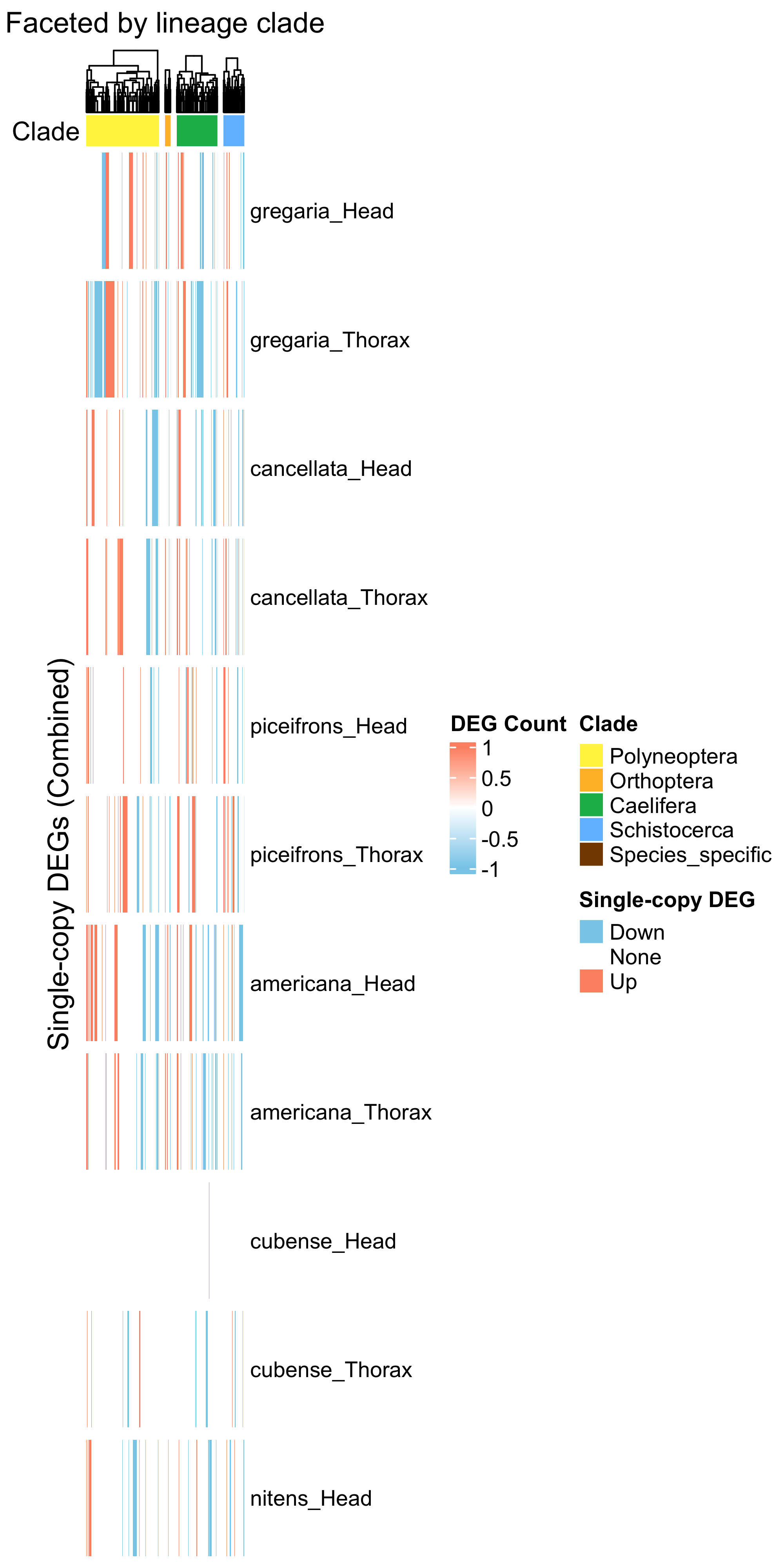
| Version | Author | Date |
|---|---|---|
| a2d2955 | Maeva TECHER | 2025-07-01 |
draw(ht_multi, annotation_legend_list = list(legend_ramp))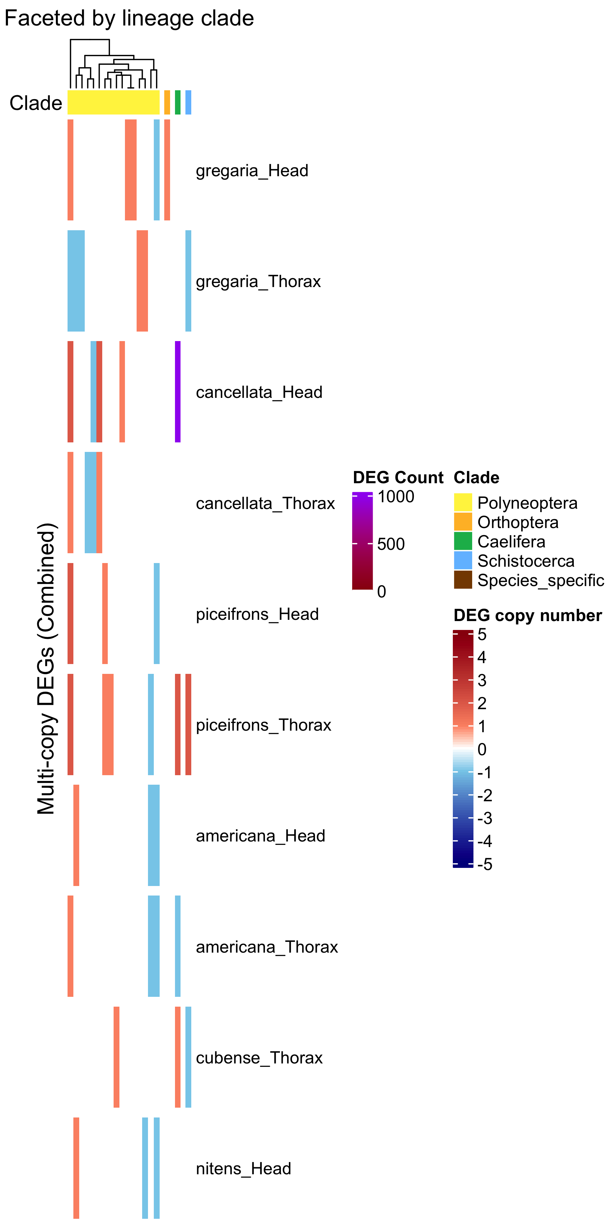
| Version | Author | Date |
|---|---|---|
| a2d2955 | Maeva TECHER | 2025-07-01 |
draw(ht_contrast, annotation_legend_list = list(leg_combined))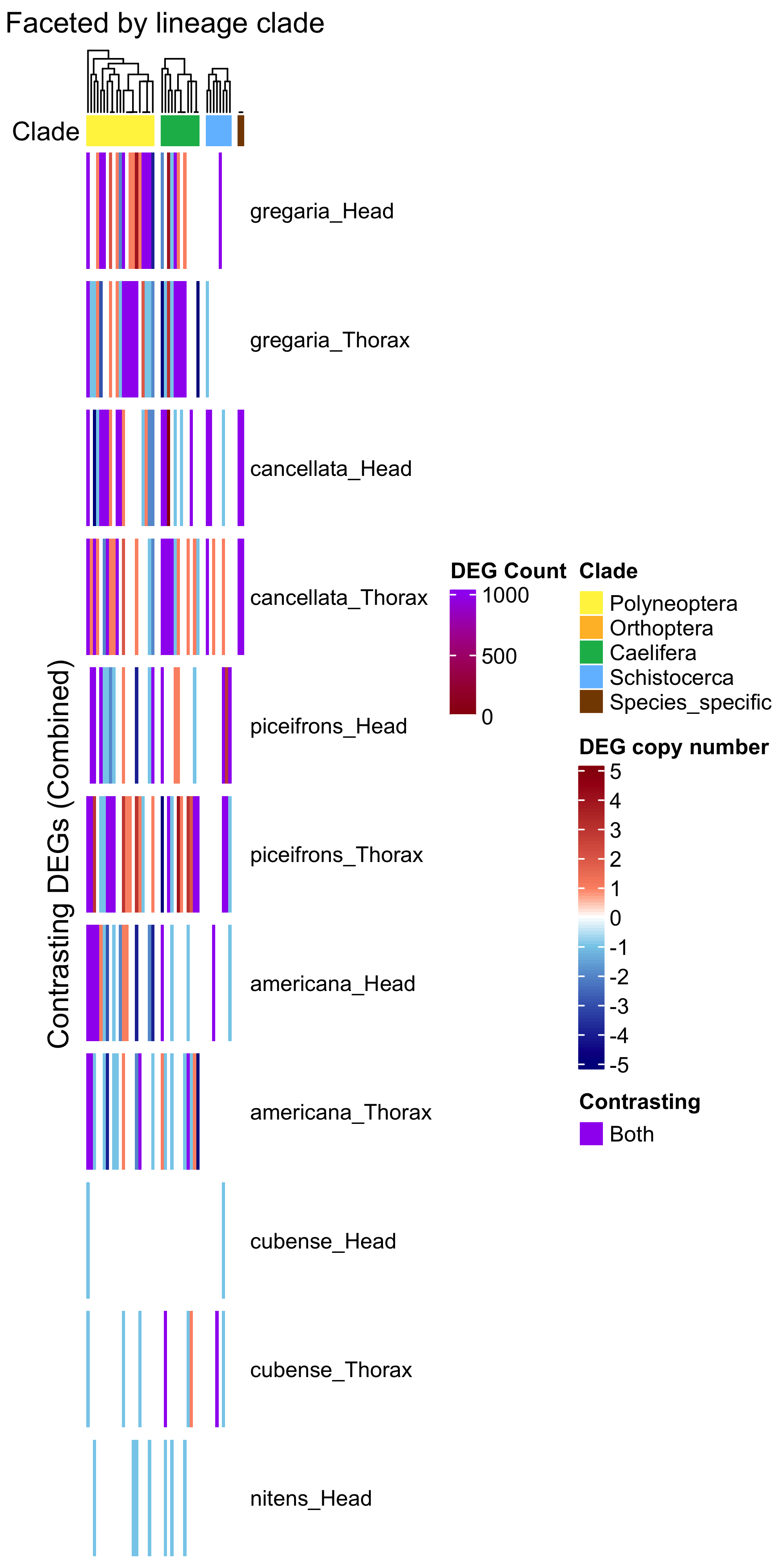
| Version | Author | Date |
|---|---|---|
| a2d2955 | Maeva TECHER | 2025-07-01 |
sessionInfo()R version 4.4.2 (2024-10-31)
Platform: aarch64-apple-darwin20
Running under: macOS Sequoia 15.5
Matrix products: default
BLAS: /Library/Frameworks/R.framework/Versions/4.4-arm64/Resources/lib/libRblas.0.dylib
LAPACK: /Library/Frameworks/R.framework/Versions/4.4-arm64/Resources/lib/libRlapack.dylib; LAPACK version 3.12.0
locale:
[1] en_US.UTF-8/en_US.UTF-8/en_US.UTF-8/C/en_US.UTF-8/en_US.UTF-8
time zone: Asia/Tokyo
tzcode source: internal
attached base packages:
[1] grid stats graphics grDevices utils datasets methods
[8] base
other attached packages:
[1] patchwork_1.3.1 circlize_0.4.16 ComplexHeatmap_2.22.0
[4] DT_0.33 kableExtra_1.4.0 lubridate_1.9.4
[7] dplyr_1.1.4 ggplot2_3.5.2 tidyverse_2.0.0
[10] forcats_1.0.0 tibble_3.3.0 purrr_1.0.4
[13] stringr_1.5.1 readr_2.1.5 tidyr_1.3.1
[16] workflowr_1.7.1
loaded via a namespace (and not attached):
[1] tidyselect_1.2.1 viridisLite_0.4.2 farver_2.1.2
[4] fastmap_1.2.0 promises_1.3.3 digest_0.6.37
[7] timechange_0.3.0 lifecycle_1.0.4 cluster_2.1.8.1
[10] Cairo_1.6-2 processx_3.8.6 magrittr_2.0.3
[13] compiler_4.4.2 rlang_1.1.6 sass_0.4.10
[16] tools_4.4.2 utf8_1.2.6 yaml_2.3.10
[19] knitr_1.50 labeling_0.4.3 htmlwidgets_1.6.4
[22] bit_4.6.0 xml2_1.3.8 RColorBrewer_1.1-3
[25] withr_3.0.2 BiocGenerics_0.52.0 stats4_4.4.2
[28] git2r_0.36.2 colorspace_2.1-1 scales_1.4.0
[31] iterators_1.0.14 dichromat_2.0-0.1 cli_3.6.5
[34] rmarkdown_2.29 crayon_1.5.3 generics_0.1.4
[37] rstudioapi_0.17.1 httr_1.4.7 tzdb_0.5.0
[40] rjson_0.2.23 cachem_1.1.0 parallel_4.4.2
[43] matrixStats_1.5.0 vctrs_0.6.5 jsonlite_2.0.0
[46] callr_3.7.6 IRanges_2.40.1 hms_1.1.3
[49] GetoptLong_1.0.5 S4Vectors_0.44.0 bit64_4.6.0-1
[52] clue_0.3-66 magick_2.8.7 crosstalk_1.2.1
[55] systemfonts_1.2.3 foreach_1.5.2 jquerylib_0.1.4
[58] glue_1.8.0 codetools_0.2-20 ps_1.9.1
[61] stringi_1.8.7 gtable_0.3.6 shape_1.4.6.1
[64] later_1.4.2 pillar_1.10.2 htmltools_0.5.8.1
[67] R6_2.6.1 textshaping_1.0.1 doParallel_1.0.17
[70] rprojroot_2.0.4 vroom_1.6.5 evaluate_1.0.4
[73] png_0.1-8 httpuv_1.6.16 bslib_0.9.0
[76] Rcpp_1.0.14 svglite_2.2.1 whisker_0.4.1
[79] xfun_0.52 fs_1.6.6 getPass_0.2-4
[82] pkgconfig_2.0.3 GlobalOptions_0.1.2