Last updated: 2020-11-17

Checks: 7 0

Knit directory: Cant_eMLR/

This reproducible R Markdown analysis was created with workflowr (version 1.6.2). The Checks tab describes the reproducibility checks that were applied when the results were created. The Past versions tab lists the development history.

R Markdown file: up-to-date

Great! Since the R Markdown file has been committed to the Git repository, you know the exact version of the code that produced these results.

Environment: empty

Great job! The global environment was empty. Objects defined in the global environment can affect the analysis in your R Markdown file in unknown ways. For reproduciblity it’s best to always run the code in an empty environment.

Seed: set.seed(20200707)

The command set.seed(20200707) was run prior to running the code in the R Markdown file. Setting a seed ensures that any results that rely on randomness, e.g. subsampling or permutations, are reproducible.

Session information: recorded

Great job! Recording the operating system, R version, and package versions is critical for reproducibility.

Cache: none

Nice! There were no cached chunks for this analysis, so you can be confident that you successfully produced the results during this run.

File paths: relative

Great job! Using relative paths to the files within your workflowr project makes it easier to run your code on other machines.

Repository version: 66fbc5d

Great! You are using Git for version control. Tracking code development and connecting the code version to the results is critical for reproducibility.

The results in this page were generated with repository version 66fbc5d. See the Past versions tab to see a history of the changes made to the R Markdown and HTML files.

Note that you need to be careful to ensure that all relevant files for the analysis have been committed to Git prior to generating the results (you can use wflow_publish or wflow_git_commit). workflowr only checks the R Markdown file, but you know if there are other scripts or data files that it depends on. Below is the status of the Git repository when the results were generated:


Ignored files:
    Ignored:    .Rproj.user/
    Ignored:    data/WOCE/
    Ignored:    data/World_Ocean_Atlas_2013_Clement/
    Ignored:    data/auxillary/
    Ignored:    data/eMLR/
    Ignored:    data/input/
    Ignored:    data/interim/
    Ignored:    data/mapping/
    Ignored:    data/output/
    Ignored:    dump/

Untracked files:
    Untracked:  output/figure/analysis_this_study/

Unstaged changes:
    Modified:   analysis/analysis_this_study.Rmd
    Modified:   analysis/read_GLODAPv2_2016_MappedClimatologies.Rmd
    Modified:   analysis/read_GLODAPv2_2020.Rmd
    Modified:   code/plotting_functions.R

Note that any generated files, e.g. HTML, png, CSS, etc., are not included in this status report because it is ok for generated content to have uncommitted changes.

These are the previous versions of the repository in which changes were made to the R Markdown (analysis/read_World_Ocean_Atlas_2018.Rmd) and HTML (docs/read_World_Ocean_Atlas_2018.html) files. If you’ve configured a remote Git repository (see ?wflow_git_remote), click on the hyperlinks in the table below to view the files as they were in that past version.

File	Version	Author	Date	Message
Rmd	66fbc5d	jens-daniel-mueller	2020-11-17	new data folder structure and modified plots and subsetting
html	42a2c82	jens-daniel-mueller	2020-11-10	Build site.
Rmd	b13b596	jens-daniel-mueller	2020-11-10	create and apply global base map layer
html	fc70a34	jens-daniel-mueller	2020-11-10	Build site.
html	b170b79	jens-daniel-mueller	2020-11-03	Build site.
Rmd	bfa7a21	jens-daniel-mueller	2020-11-03	added comparison to Gruber 2019, revised basin mask
html	411a35b	jens-daniel-mueller	2020-10-02	Build site.
html	0d38979	jens-daniel-mueller	2020-10-01	Build site.
html	4578cfa	jens-daniel-mueller	2020-09-19	Build site.
html	d59f716	jens-daniel-mueller	2020-09-18	Build site.
html	f5a20ac	jens-daniel-mueller	2020-09-17	Build site.
html	cf64460	jens-daniel-mueller	2020-09-17	Build site.
html	d43d9e2	jens-daniel-mueller	2020-09-16	Build site.
html	1f3319a	jens-daniel-mueller	2020-09-16	Build site.
html	0aa596d	jens-daniel-mueller	2020-09-16	Build site.
Rmd	fb6a3c3	jens-daniel-mueller	2020-09-16	created surface water climatology
html	da91d98	jens-daniel-mueller	2020-09-10	Build site.
html	4c73801	jens-daniel-mueller	2020-09-10	Build site.
Rmd	da66d06	jens-daniel-mueller	2020-09-10	global section plots modified
html	5e9663c	jens-daniel-mueller	2020-09-10	Build site.
Rmd	5c58ade	jens-daniel-mueller	2020-09-10	global section included on maps
html	541d383	jens-daniel-mueller	2020-09-10	Build site.
Rmd	8001403	jens-daniel-mueller	2020-09-10	changed to global section plots
html	a34a239	jens-daniel-mueller	2020-09-10	Build site.
Rmd	143fbd7	jens-daniel-mueller	2020-09-10	global section plot added
html	c3ffdfd	jens-daniel-mueller	2020-09-08	Build site.
html	7e2e27c	jens-daniel-mueller	2020-09-08	Build site.
Rmd	9a1e810	jens-daniel-mueller	2020-09-08	applied depth threshold
html	1001303	jens-daniel-mueller	2020-09-08	Build site.
Rmd	08ea446	jens-daniel-mueller	2020-09-08	all subsetting during read-in
html	a50f053	jens-daniel-mueller	2020-09-07	Build site.
html	da445a6	jens-daniel-mueller	2020-09-04	Build site.
html	fa11a74	jens-daniel-mueller	2020-09-02	Build site.
html	429aab3	jens-daniel-mueller	2020-09-01	Build site.
html	f4216dd	jens-daniel-mueller	2020-09-01	Build site.
html	13a76d5	jens-daniel-mueller	2020-08-28	Build site.
html	27404de	jens-daniel-mueller	2020-08-27	Build site.
html	06c2578	jens-daniel-mueller	2020-08-27	Build site.
Rmd	c54a7fc	jens-daniel-mueller	2020-08-27	updated plots
html	b6d0e6a	jens-daniel-mueller	2020-08-27	Build site.
html	f40e48b	jens-daniel-mueller	2020-08-26	Build site.
html	8f50e8e	jens-daniel-mueller	2020-08-26	Build site.
Rmd	cb33664	jens-daniel-mueller	2020-08-26	basin mask created for Indian and Pacific ocean seperately
html	ec20f40	jens-daniel-mueller	2020-08-24	Build site.
html	b6711a4	jens-daniel-mueller	2020-08-21	Build site.
Rmd	79041e4	jens-daniel-mueller	2020-08-21	removed WOA18 vertical interpolation but rather removed unnecessary depth levels
html	078df6a	jens-daniel-mueller	2020-08-21	Build site.
Rmd	d61cc23	jens-daniel-mueller	2020-08-21	gamma WOA18 calculated with pressure rather than depth, spatial boundaries applied to predictors
html	5ffe187	jens-daniel-mueller	2020-08-20	Build site.
html	6320d89	jens-daniel-mueller	2020-08-20	Build site.
Rmd	0c8e2e8	jens-daniel-mueller	2020-08-20	moved WOA 13 Clement to separate Rmd
html	1064ef8	jens-daniel-mueller	2020-08-19	Build site.
html	29a537a	jens-daniel-mueller	2020-08-18	Build site.
Rmd	7fb61d5	jens-daniel-mueller	2020-08-18	rerun with all parameters in one file
html	2c0a2c2	jens-daniel-mueller	2020-08-14	Build site.
Rmd	f6a3179	jens-daniel-mueller	2020-08-14	checked gamma calculation and sabine cant
html	a3b6b68	jens-daniel-mueller	2020-08-13	Build site.
html	00c2120	jens-daniel-mueller	2020-08-13	Build site.
html	c9df014	jens-daniel-mueller	2020-08-13	Build site.
Rmd	35b1b79	jens-daniel-mueller	2020-08-13	formatting
html	f0b8f3f	jens-daniel-mueller	2020-08-13	Build site.
Rmd	044073d	jens-daniel-mueller	2020-08-13	Arctic and Sea of Japan incuded in basin mask
html	a1b06c9	jens-daniel-mueller	2020-08-13	Build site.
Rmd	7133d1a	jens-daniel-mueller	2020-08-13	potentiell temperature calculated
html	bf69270	jens-daniel-mueller	2020-08-13	Build site.
html	1176c9a	jens-daniel-mueller	2020-08-12	Build site.
html	1a078e7	jens-daniel-mueller	2020-08-12	Build site.
Rmd	6344282	jens-daniel-mueller	2020-08-12	updated lon conversion, variable names and masks
html	2980ad4	jens-daniel-mueller	2020-08-12	Build site.
Rmd	8ba8189	jens-daniel-mueller	2020-08-12	corrected depth conversion from pressure
html	f143b2d	jens-daniel-mueller	2020-08-12	Build site.
Rmd	c78a3f9	jens-daniel-mueller	2020-08-12	corrected pressure input for gamma calculation
html	2d179e7	jens-daniel-mueller	2020-08-12	Build site.
Rmd	525cb52	jens-daniel-mueller	2020-08-12	WOA 18 gamma calculation, new lon values in mapping
html	9455a55	jens-daniel-mueller	2020-08-12	Build site.
Rmd	1a7acc2	jens-daniel-mueller	2020-08-12	applied basin mask, combined sectio plots for Atl, Pac, Ind
html	35b284d	jens-daniel-mueller	2020-08-11	Build site.
Rmd	5d45981	jens-daniel-mueller	2020-08-11	plot sal sections from function both basins
html	495debb	jens-daniel-mueller	2020-08-11	Build site.
Rmd	cfbc5e4	jens-daniel-mueller	2020-08-11	plot sections from function both basins
html	075099b	jens-daniel-mueller	2020-08-11	Build site.
Rmd	adc0335	jens-daniel-mueller	2020-08-11	plot sections from function
Rmd	69b9a78	jens-daniel-mueller	2020-08-11	plot sections from function
html	cfd84b7	jens-daniel-mueller	2020-08-11	Build site.
Rmd	ca836af	jens-daniel-mueller	2020-08-11	Removed Rmd child tests
html	dc2b649	jens-daniel-mueller	2020-08-11	Build site.
Rmd	928cd7d	jens-daniel-mueller	2020-08-11	Rmd child test with access to global object
html	be47191	jens-daniel-mueller	2020-08-11	Build site.
Rmd	9c8f6b8	jens-daniel-mueller	2020-08-11	Rmd child test with variable name transmission
html	6ebb3de	jens-daniel-mueller	2020-08-11	Build site.
Rmd	0333c99	jens-daniel-mueller	2020-08-11	test addition child Rmd file
html	fbbabf4	jens-daniel-mueller	2020-08-11	Build site.
Rmd	e92638d	jens-daniel-mueller	2020-08-11	plot maps from function
html	cee0e89	jens-daniel-mueller	2020-08-11	Build site.
Rmd	c9e2d65	jens-daniel-mueller	2020-08-11	plot maps from function
html	de933d9	jens-daniel-mueller	2020-08-11	Build site.
Rmd	c3a6c63	jens-daniel-mueller	2020-08-11	included WOA land mask and longitude conversion
html	5d33341	jens-daniel-mueller	2020-08-11	Build site.
html	8a010ca	jens-daniel-mueller	2020-08-11	Build site.
html	a01041a	jens-daniel-mueller	2020-08-11	Build site.
html	e18e59a	jens-daniel-mueller	2020-08-10	Build site.
html	7d7900a	jens-daniel-mueller	2020-08-07	Build site.
html	4394942	jens-daniel-mueller	2020-08-04	Build site.
Rmd	eb838d4	jens-daniel-mueller	2020-08-04	Read, plot, write data from D Clement
html	662560f	jens-daniel-mueller	2020-08-04	Build site.
Rmd	b2b1f24	jens-daniel-mueller	2020-08-04	Read, plot, write data from D Clement
html	e9a52c5	jens-daniel-mueller	2020-07-31	Build site.
Rmd	5ee70b2	jens-daniel-mueller	2020-07-31	formatting
html	f33772b	jens-daniel-mueller	2020-07-31	Build site.
Rmd	dea0eaf	jens-daniel-mueller	2020-07-31	alligned plots with GLODAP climatology
html	9dc5d7f	jens-daniel-mueller	2020-07-29	Build site.
html	21524b4	jens-daniel-mueller	2020-07-29	Build site.
html	f5c4667	jens-daniel-mueller	2020-07-29	Build site.
Rmd	f6d4d92	jens-daniel-mueller	2020-07-29	format and plots revised
html	8d71a56	jens-daniel-mueller	2020-07-29	Build site.
Rmd	82db969	jens-daniel-mueller	2020-07-29	format and plots revised
html	2e08795	jens-daniel-mueller	2020-07-24	Build site.
html	61a1a48	jens-daniel-mueller	2020-07-24	Build site.
Rmd	864a6e3	jens-daniel-mueller	2020-07-24	merged predictor data sets
html	eb716ce	jens-daniel-mueller	2020-07-23	Build site.
Rmd	ffd46da	jens-daniel-mueller	2020-07-23	WOA18 read in
html	556e6cc	jens-daniel-mueller	2020-07-23	Build site.
html	c1289a2	jens-daniel-mueller	2020-07-23	Build site.
html	2890e73	jens-daniel-mueller	2020-07-23	Build site.
html	fdfa7b9	jens-daniel-mueller	2020-07-22	Build site.
html	bb9c002	jens-daniel-mueller	2020-07-21	Build site.
Rmd	d2ed0f8	jens-daniel-mueller	2020-07-21	harmonied lat lon labeling
html	97dbf5b	jens-daniel-mueller	2020-07-21	Build site.
Rmd	5def7e8	jens-daniel-mueller	2020-07-21	create csvs for each parameter
html	b47adc2	jens-daniel-mueller	2020-07-20	Build site.
Rmd	366d7d5	jens-daniel-mueller	2020-07-20	update plots
html	1de1bc0	jens-daniel-mueller	2020-07-20	Build site.
Rmd	68e4615	jens-daniel-mueller	2020-07-20	assigned ocean basins and plotted world map
html	3149ffd	jens-daniel-mueller	2020-07-20	Build site.
Rmd	918f8c8	jens-daniel-mueller	2020-07-20	assigned ocean basins and plotted world map
html	2fa2896	jens-daniel-mueller	2020-07-20	Build site.
Rmd	23220a8	jens-daniel-mueller	2020-07-20	assigned ocean basins and plotted world map
html	27d380d	jens-daniel-mueller	2020-07-20	Build site.
Rmd	09f3f73	jens-daniel-mueller	2020-07-20	basin masks read in
html	22b588c	jens-daniel-mueller	2020-07-18	Build site.
Rmd	87a4680	jens-daniel-mueller	2020-07-18	added WOA blank script

library(tidyverse)
library(tidync)
library(reticulate)
library(oce)
library(gsw)
library(geosphere)
library(patchwork)

1 Data source

Data source: World Ocean Atlas 2018

2 Masks

2.1 Land

2.1.1 Read mask

The land sea mask with 1x1° resolution from the file landsea_01.msk was used.

landsea_01 <- read_csv(here::here("data/input/World_Ocean_Atlas_2018",
                                  "landsea_01.msk"),
                         skip = 1,
                         col_types = list(.default = "d"))

2.1.2 Label

According to the WOA18 documentation document:

“The landsea_XX.msk contains the standard depth level number at which the bottom of the ocean is first encountered at each quarter-degree or one-degree square for the entire world. Land will have a value of 1, corresponding to the surface.”

The landmask was derived as coordinates with value 1.

landmask <- landsea_01 %>% 
  mutate(region = if_else(Bottom_Standard_Level == "1",
                         "land", "ocean")) %>% 
  select(-Bottom_Standard_Level)

landmask <- landmask %>% 
  rename(lat = Latitude,
         lon = Longitude) %>% 
  mutate(lon = if_else(lon < 20, lon + 360, lon))

landmask <- landmask %>%
  filter(region == "land", 
         lat >= parameters$lat_min,
         lat <= parameters$lat_max) %>% 
  select(-region)

rm(landsea_01)

2.2 Basins

2.2.1 Read mask

The surface mask (0m) with 1x1° resolution from the file basinmask_01.msk was used.

basinmask_01 <- read_csv(here::here("data/input/World_Ocean_Atlas_2018",
                                    "basinmask_01.msk"),
                         skip = 1,
                         col_types = list(.default = "d"))

basinmask_01 <- basinmask_01 %>% 
  select(Latitude:Basin_0m) %>% 
  mutate(Basin_0m = as.factor(Basin_0m)) %>% 
  rename(lat = Latitude, lon = Longitude)

2.2.2 Labels

According to WOA FAQ website and WOA18 documentation, number codes in the mask files were used to assign ocean basins as follows:

Atlantic Ocean:

1: Atlantic Ocean
10: Southern Ocean between 63°W and 20°E
11: Arctic Ocean (restricted by northern latitude limit 65N)

Indian Ocean:

3: Indian Ocean
10: Southern Ocean between 20°E and 147°E

Pacific Ocean:

2: Pacific Ocean
10: Southern Ocean between 147°E and 63°W
12: Sea of Japan
56: Bay of Bengal

For eMLR model fitting and mapping, Indian and Pacific Ocean were combined as Indo-Pacific.

basinmask_01 <- basinmask_01 %>%
  filter(Basin_0m %in% c("1", "2", "3", "10", "11", "12", "56"),
         lat <= parameters$lat_max) %>%
  mutate(
    basin_AIP = "none",
    basin_AIP = case_when(
      Basin_0m == "1" ~ "Atlantic",
      Basin_0m == "10" & lon >= -63 & lon < 20 ~ "Atlantic",
      Basin_0m == "11" ~ "Atlantic",
      Basin_0m == "3" ~ "Indian",
      Basin_0m == "56" ~ "Indian",
      Basin_0m == "10" & lon >= 20 & lon < 147 ~ "Indian",
      Basin_0m == "2" ~ "Pacific",
      Basin_0m == "12" ~ "Pacific",
      Basin_0m == "10" &
        lon >= 147 | lon < -63 ~ "Pacific"
    )
  ) %>%
  mutate(basin = if_else(basin_AIP == "Atlantic",
                         "Atlantic",
                         "Indo-Pacific")) %>%
  select(-Basin_0m) %>%
  mutate(lon = if_else(lon < 20, lon + 360, lon))

2.2.3 Map

map <- 
  ggplot() +
  geom_raster(data = landmask,
              aes(lon, lat), fill = "grey80") +
  coord_quickmap(expand = 0) +
  theme(axis.title = element_blank())

map +
  geom_raster(data = basinmask_01,
              aes(lon, lat, fill = basin_AIP)) +
  scale_fill_brewer(palette = "Dark2") +
  theme(legend.position = "top",
        legend.title = element_blank())

map %>%  
  write_rds(here::here("data/auxillary",
                       "map_landmask_WOA18.rds"))

2.3 Global section

To plot sections from the North Atlantic south to the Southern Ocean, around Antartica and back North across the Pacific Ocean, corresponding coordinates were subsetted from the basin mask and distances between coordinate grid points calculated.

section <- basinmask_01 %>%
  select(lon, lat)

Atl_NS <- section %>%
  filter(
    lon == parameters$lon_Atl_section,
    lat <= parameters$lat_section_N,
    lat >= parameters$lat_section_S
  ) %>%
  arrange(-lat)

Atl_SO <- section %>%
  filter(lon > parameters$lon_Atl_section,
         lat == parameters$lat_section_S) %>%
  arrange(lon)

Pac_SO <- section %>%
  filter(lon < parameters$lon_Pac_section,
         lat == parameters$lat_section_S) %>%
  arrange(lon)

Pac_SN <- section %>%
  filter(
    lon == parameters$lon_Pac_section,
    lat <= parameters$lat_section_N,
    lat >= parameters$lat_section_S
  ) %>%
  arrange(lat)

section_global_coordinates <- bind_rows(Atl_NS,
                     Atl_SO,
                     Pac_SO,
                     Pac_SN)

section_global_coordinates <- section_global_coordinates %>%
  mutate(lon_180 = if_else(lon > 180, lon - 360, lon))

section_global_coordinates <- section_global_coordinates %>%
  mutate(dist_int = distGeo(cbind(lon_180, lat)) / 1e6) %>%
  mutate(dist = cumsum(dist_int))


section_global_coordinates <- section_global_coordinates %>%
  select(lon, lat, dist) %>% 
  drop_na()

rm(Atl_NS, Atl_SO, Pac_SN, Pac_SO, section)

map +
  geom_point(data = section_global_coordinates,
             aes(lon, lat, col = dist)) +
  scale_colour_viridis_b(name = "Distance (Mm)") +
  theme(legend.position = "top")

2.4 Write files

# basinmask_01 %>% 
#   select(-basin) %>% 
#   write_csv(here::here("data/auxillary",
#                        "basin_mask_WOA18_AIP.csv"))

basinmask_01 %>% 
  #select(-basin_AIP) %>% 
  write_csv(here::here("data/auxillary",
                       "basin_mask_WOA18.csv"))

landmask %>% 
  write_csv(here::here("data/auxillary",
                       "land_mask_WOA18.csv"))

section_global_coordinates %>%
  write_csv(here::here("data/auxillary",
                       "section_global_coordinates.csv"))

3 Climatologies

Copied from the WOA FAQ website, the file naming conventions is:

PREF_DDDD_VTTFFGG.EXT, where:

PREF: prefix
DDDD: decade
V: variable
TT: time period
FF: field type
GG: grid (5deg- 5°, 01- 1°, 04 - 1/4°)
EXT: file extention

Short description of two statistical fields in WOA

Objectively analyzed climatologies are the objectively interpolated mean fields for oceanographic variables at standard - depth levels for the World Ocean.
The statistical mean is the average of all unflagged interpolated values at each standard depth level for each variable - in each 1° square which contains at least one measurement for the given oceanographic variable.

Here, we use

Fields: objectively analyzed mean
Decades: all decades
Grid: 1 deg resolution

According to the WOA18 documentation document:

What are the units for temperature and salinity in the WOA18?

In situ temperatures used for WOA18 are not converted from their original scale, so there is a mix of IPTS-48, IPTS-68, and ITS-90 (and pre IPTS-48 temperatures). The differences between scales are small (on the order of 0.01°C) and should not have much effect on the climatological means, except, possibly at very deep depths. Values for salinity are on the Practical salinity scale (PSS-78). Pre-1978 salinity values converted from conductivity may have used a different salinity scale. Pre-conductivity salinities use the Knudsen method.

3.1 Read ncdfs

# temperature

WOA18_tem <- tidync(here::here("data/input/World_Ocean_Atlas_2018",
                                 "woa18_decav_t00_01.nc"))

WOA18_tem_tibble <- WOA18_tem %>% hyper_tibble()

WOA18_tem_tibble <- WOA18_tem_tibble  %>% 
  select(tem = t_an, lon, lat, depth) %>% 
  drop_na() %>% 
  mutate(lon = if_else(lon < 20, lon + 360, lon))

# salinity

WOA18_sal <- tidync(here::here("data/input/World_Ocean_Atlas_2018",
                                 "woa18_decav_s00_01.nc"))

WOA18_sal_tibble <- WOA18_sal %>% hyper_tibble()

WOA18_sal_tibble <- WOA18_sal_tibble  %>% 
  select(sal = s_an, lon, lat, depth) %>% 
  drop_na() %>% 
  mutate(lon = if_else(lon < 20, lon + 360, lon))

rm(WOA18_sal, WOA18_tem)

WOA18_sal_tem <- full_join(WOA18_sal_tibble, WOA18_tem_tibble)
rm(WOA18_sal_tibble, WOA18_tem_tibble)

3.2 Apply basin mask

Data outside the WOA18 basin mask were removed for further analysis.

WOA18_sal_tem <- inner_join(WOA18_sal_tem, basinmask_01)

3.3 Apply spatial boundaries

Following limits were considered but are currently not applied:

minimum bottom depth: 500m

WOA18_sal_tem_grid <- WOA18_sal_tem %>% 
  group_by(lat, lon) %>% 
  summarise(bottomdepth = max(depth)) %>% 
  ungroup()

WOA18_sal_tem_grid <- WOA18_sal_tem_grid %>% 
  filter(bottomdepth >= parameters$bottomdepth_min) %>% 
  select(-bottomdepth)

WOA18_sal_tem <- left_join(WOA18_sal_tem_grid, WOA18_sal_tem)

maximum depth: 3000m

WOA18_sal_tem <- WOA18_sal_tem %>% 
  filter(depth <= parameters$inventory_depth)

3.4 Potential temperature

3.4.1 Calculation

WOA18_sal_tem <- WOA18_sal_tem %>% 
  mutate(THETA = swTheta(salinity = sal,
                         temperature = tem,
                         pressure = depth,
                         referencePressure = 0,
                         longitude = lon - 180,
                         latitude = lat))

3.4.2 Profile

Example profile from North Atlantic Ocean.

WOA18_sal_tem %>%
  filter(lat == parameters$lat_Atl_profile,
         lon == parameters$lon_Atl_section) %>%
  ggplot() +
  geom_line(aes(tem, depth, col = "insitu")) +
  geom_point(aes(tem, depth, col = "insitu")) +
  geom_line(aes(THETA, depth, col = "theta")) +
  geom_point(aes(THETA, depth, col = "theta")) +
  scale_y_reverse() +
  scale_color_brewer(palette = "Dark2", name = "Scale")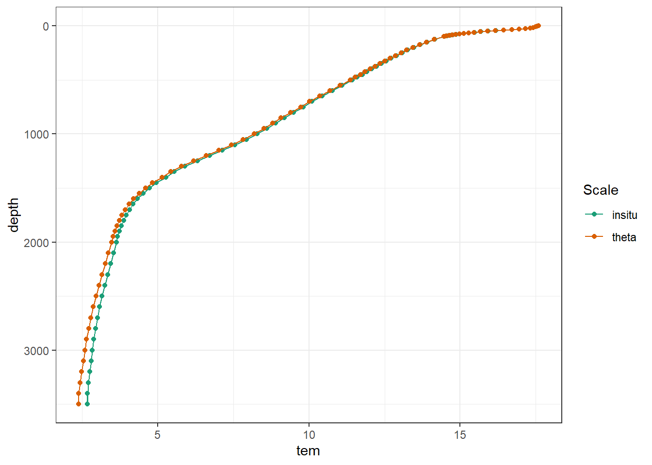

3.4.3 Section

section_global_coordinates <-
  read_csv(here::here("data/auxillary",
                      "section_global_coordinates.csv"))

section_global(WOA18_sal_tem,
               "THETA",
               "Global climatological section")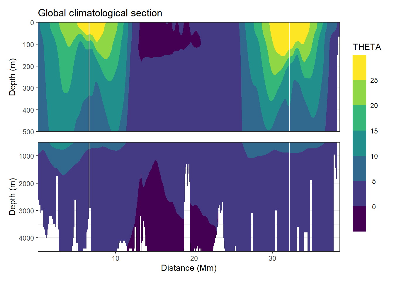

3.5 Neutral density

Neutral density gamma was calculated with a Python script provided by Serazin et al (2011), which performs a polynomial approximation of the original gamma calculation.

3.5.1 Calculation

# calculate pressure from depth

WOA18_sal_tem <- WOA18_sal_tem %>% 
  mutate(CTDPRS = gsw_p_from_z(-depth,
                               lat))
# rename variables according to python script

WOA18_sal_tem_gamma_prep <- WOA18_sal_tem %>% 
  rename(LATITUDE = lat,
         LONGITUDE = lon,
         SALNTY = sal)

# load python scripts

source_python(here::here("code/python_scripts",
                         "Gamma_GLODAP_python.py"))

# calculate gamma

WOA18_sal_tem_gamma_calc <- calculate_gamma(WOA18_sal_tem_gamma_prep)

# reverse variable naming

WOA18_sal_tem <- WOA18_sal_tem_gamma_calc %>% 
  select(-c(CTDPRS, THETA)) %>% 
  rename(lat = LATITUDE,
         lon = LONGITUDE,
         sal = SALNTY,
         gamma  = GAMMA)

WOA18_sal_tem <- as_tibble(WOA18_sal_tem)

rm(WOA18_sal_tem_gamma_calc, WOA18_sal_tem_gamma_prep)

3.5.2 Apply density threshold

The predictor field was split into two parts:

Deep water: neutral densities >= 26 and depth >= 150m
Shallow water: rest

WOA18_sal_tem_surface <- WOA18_sal_tem %>%
  filter(depth < parameters$depth_min,
         gamma < parameters$gamma_min)

WOA18_sal_tem <- WOA18_sal_tem %>%
  filter(depth >= parameters$depth_min | gamma >= parameters$gamma_min)

3.5.3 Write/open file

WOA18_sal_tem %>% 
  write_csv(here::here("data/interim/predictor_climatologies",
                       "WOA18_sal_tem.csv"))

WOA18_sal_tem_surface %>%
  write_csv(here::here("data/interim/predictor_climatologies",
                       "WOA18_sal_tem_surface.csv"))

3.6 Temperature plots

Below, following subsets of the climatologies are plotted for all relevant parameters:

Horizontal planes at 0, 150, 500, 2000m
Meridional sections at longitudes: 335.5, 190.5, 70.5

Section locations are indicated as white lines in maps.

3.6.1 Surface map

map_climatology(WOA18_sal_tem, "tem")

3.6.2 Section

section_global(WOA18_sal_tem,
               "tem",
               "Global climatological section")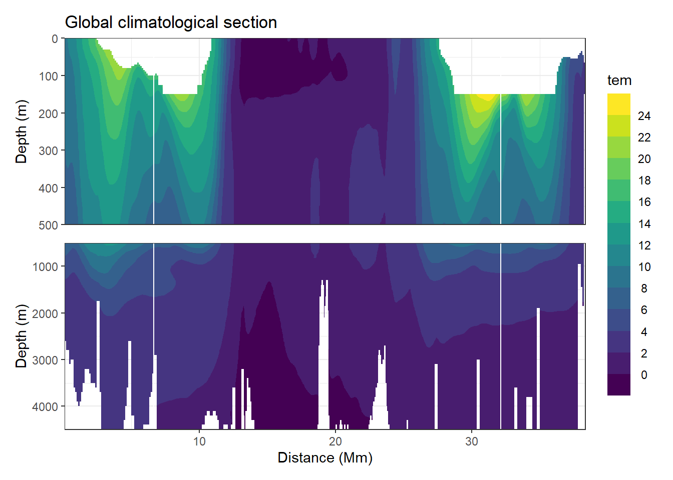

3.7 Salinity plots

3.7.1 Surface map

map_climatology(WOA18_sal_tem,
                "sal")

3.7.2 Section

section_global(WOA18_sal_tem,
               "sal",
               "Global climatological section")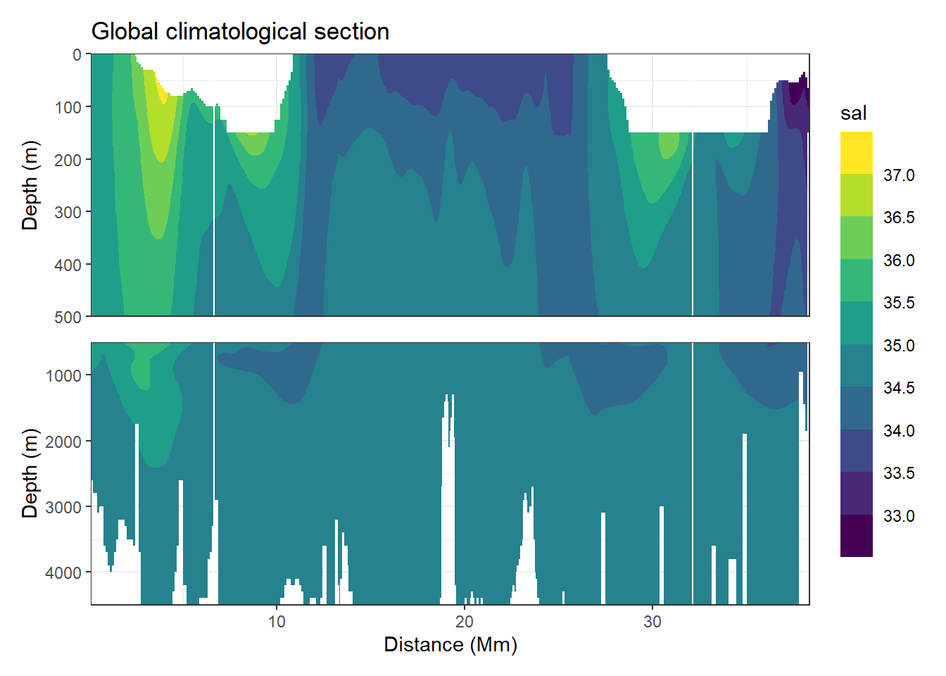

3.8 Neutral density plots

3.8.1 Surface map

map_climatology(WOA18_sal_tem, "gamma")

3.8.2 Section

section_global(WOA18_sal_tem, "gamma",
               "Global climatological section")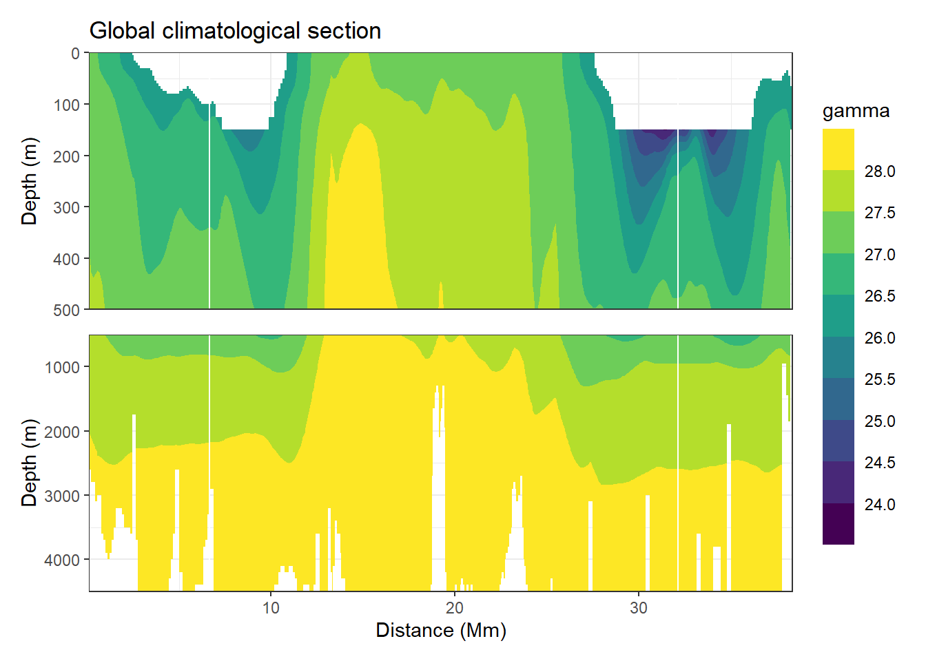

3.8.3 Surface map shallow

map_climatology(WOA18_sal_tem_surface, "gamma")

3.8.4 Section shallow

section_global(WOA18_sal_tem_surface, "gamma",
               "Global climatological section")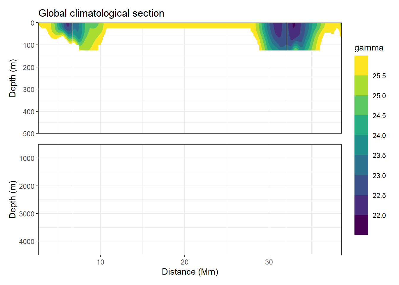

sessionInfo()

R version 4.0.2 (2020-06-22)
Platform: x86_64-w64-mingw32/x64 (64-bit)
Running under: Windows 10 x64 (build 18363)

Matrix products: default

locale:
[1] LC_COLLATE=English_Germany.1252  LC_CTYPE=English_Germany.1252   
[3] LC_MONETARY=English_Germany.1252 LC_NUMERIC=C                    
[5] LC_TIME=English_Germany.1252    

attached base packages:
[1] stats     graphics  grDevices utils     datasets  methods   base     

other attached packages:
 [1] patchwork_1.0.1  geosphere_1.5-10 oce_1.2-0        gsw_1.0-5       
 [5] testthat_2.3.2   reticulate_1.16  tidync_0.2.4     forcats_0.5.0   
 [9] stringr_1.4.0    dplyr_1.0.0      purrr_0.3.4      readr_1.3.1     
[13] tidyr_1.1.0      tibble_3.0.3     ggplot2_3.3.2    tidyverse_1.3.0 
[17] workflowr_1.6.2 

loaded via a namespace (and not attached):
 [1] httr_1.4.2         viridisLite_0.3.0  jsonlite_1.7.0     here_0.1          
 [5] modelr_0.1.8       assertthat_0.2.1   sp_1.4-2           blob_1.2.1        
 [9] cellranger_1.1.0   yaml_2.2.1         pillar_1.4.6       backports_1.1.8   
[13] lattice_0.20-41    glue_1.4.1         digest_0.6.25      RColorBrewer_1.1-2
[17] promises_1.1.1     rvest_0.3.6        colorspace_1.4-1   htmltools_0.5.0   
[21] httpuv_1.5.4       Matrix_1.2-18      pkgconfig_2.0.3    broom_0.7.0       
[25] haven_2.3.1        scales_1.1.1       whisker_0.4        later_1.1.0.1     
[29] git2r_0.27.1       farver_2.0.3       generics_0.0.2     ellipsis_0.3.1    
[33] withr_2.2.0        cli_2.0.2          magrittr_1.5       crayon_1.3.4      
[37] readxl_1.3.1       evaluate_0.14      fs_1.4.2           ncdf4_1.17        
[41] fansi_0.4.1        xml2_1.3.2         tools_4.0.2        hms_0.5.3         
[45] lifecycle_0.2.0    munsell_0.5.0      reprex_0.3.0       isoband_0.2.2     
[49] compiler_4.0.2     RNetCDF_2.3-1      rlang_0.4.7        grid_4.0.2        
[53] rstudioapi_0.11    rappdirs_0.3.1     labeling_0.3       rmarkdown_2.3     
[57] gtable_0.3.0       DBI_1.1.0          R6_2.4.1           ncmeta_0.2.5      
[61] lubridate_1.7.9    knitr_1.30         rprojroot_1.3-2    stringi_1.4.6     
[65] Rcpp_1.0.5         vctrs_0.3.2        dbplyr_1.4.4       tidyselect_1.1.0  
[69] xfun_0.16

World Ocean Atlas 2018

Jens Daniel Müller

17 November, 2020