GLODAPv2_2020
Jens Daniel Müller
13 August, 2020
Last updated: 2020-08-13
Checks: 7 0
Knit directory: Cant_eMLR/
This reproducible R Markdown analysis was created with workflowr (version 1.6.2). The Checks tab describes the reproducibility checks that were applied when the results were created. The Past versions tab lists the development history.
Great! Since the R Markdown file has been committed to the Git repository, you know the exact version of the code that produced these results.
Great job! The global environment was empty. Objects defined in the global environment can affect the analysis in your R Markdown file in unknown ways. For reproduciblity it’s best to always run the code in an empty environment.
The command set.seed(20200707) was run prior to running the code in the R Markdown file. Setting a seed ensures that any results that rely on randomness, e.g. subsampling or permutations, are reproducible.
Great job! Recording the operating system, R version, and package versions is critical for reproducibility.
Nice! There were no cached chunks for this analysis, so you can be confident that you successfully produced the results during this run.
Great job! Using relative paths to the files within your workflowr project makes it easier to run your code on other machines.
Great! You are using Git for version control. Tracking code development and connecting the code version to the results is critical for reproducibility.
The results in this page were generated with repository version 47e19d8. See the Past versions tab to see a history of the changes made to the R Markdown and HTML files.
Note that you need to be careful to ensure that all relevant files for the analysis have been committed to Git prior to generating the results (you can use wflow_publish or wflow_git_commit). workflowr only checks the R Markdown file, but you know if there are other scripts or data files that it depends on. Below is the status of the Git repository when the results were generated:
Ignored files:
    Ignored:    .Rproj.user/
    Ignored:    data/GLODAPv1_1/
    Ignored:    data/GLODAPv2_2016b_MappedClimatologies/
    Ignored:    data/GLODAPv2_2020/
    Ignored:    data/Gruber_2019/
    Ignored:    data/WOCE/
    Ignored:    data/World_Ocean_Atlas_2018/
    Ignored:    data/dclement/
    Ignored:    data/eMLR/
    Ignored:    data/mapping/
    Ignored:    data/pCO2_atmosphere/
    Ignored:    data/parameters/
    Ignored:    dump/
    Ignored:    figure/

Unstaged changes:
    Modified:   analysis/_site.yml
    Modified:   analysis/config_parameterization.Rmd
Note that any generated files, e.g. HTML, png, CSS, etc., are not included in this status report because it is ok for generated content to have uncommitted changes.
These are the previous versions of the repository in which changes were made to the R Markdown (analysis/read_GLODAPv2_2020.Rmd) and HTML (docs/read_GLODAPv2_2020.html) files. If you’ve configured a remote Git repository (see ?wflow_git_remote), click on the hyperlinks in the table below to view the files as they were in that past version.
| File | Version | Author | Date | Message |
|---|---|---|---|---|
| html | 1176c9a | jens-daniel-mueller | 2020-08-12 | Build site. |
| html | 1a078e7 | jens-daniel-mueller | 2020-08-12 | Build site. |
| Rmd | 6344282 | jens-daniel-mueller | 2020-08-12 | updated lon conversion, variable names and masks |
| html | f143b2d | jens-daniel-mueller | 2020-08-12 | Build site. |
| html | 2d179e7 | jens-daniel-mueller | 2020-08-12 | Build site. |
| html | 5d33341 | jens-daniel-mueller | 2020-08-11 | Build site. |
| html | 8a010ca | jens-daniel-mueller | 2020-08-11 | Build site. |
| html | a01041a | jens-daniel-mueller | 2020-08-11 | Build site. |
| html | 1b3f5e2 | jens-daniel-mueller | 2020-08-11 | Build site. |
| Rmd | e646f85 | jens-daniel-mueller | 2020-08-11 | parameterization in separate file |
| html | e18e59a | jens-daniel-mueller | 2020-08-10 | Build site. |
| html | 7d7900a | jens-daniel-mueller | 2020-08-07 | Build site. |
| html | ddf44d7 | jens-daniel-mueller | 2020-07-31 | Build site. |
| Rmd | b4fa5a8 | jens-daniel-mueller | 2020-07-31 | link to all cruise plots included |
| html | 243f31c | jens-daniel-mueller | 2020-07-31 | Build site. |
| Rmd | 977782e | jens-daniel-mueller | 2020-07-31 | minor plot update, open questions added |
| html | 9dc5d7f | jens-daniel-mueller | 2020-07-29 | Build site. |
| html | 21524b4 | jens-daniel-mueller | 2020-07-29 | Build site. |
| html | ff17968 | jens-daniel-mueller | 2020-07-29 | Build site. |
| Rmd | cb5074e | jens-daniel-mueller | 2020-07-29 | subset Cant to GLODAP before merging |
| html | 8d71a56 | jens-daniel-mueller | 2020-07-29 | Build site. |
| Rmd | 82db969 | jens-daniel-mueller | 2020-07-29 | format and plots revised |
| html | 2e2412d | jens-daniel-mueller | 2020-07-29 | Build site. |
| Rmd | a9fbf3a | jens-daniel-mueller | 2020-07-29 | formating |
| html | 5274d0b | jens-daniel-mueller | 2020-07-29 | Build site. |
| Rmd | 304aa74 | jens-daniel-mueller | 2020-07-29 | plot improvements |
| html | 75da185 | jens-daniel-mueller | 2020-07-29 | Build site. |
| Rmd | 26db597 | jens-daniel-mueller | 2020-07-29 | cleaned code and output |
| html | 2e08795 | jens-daniel-mueller | 2020-07-24 | Build site. |
| html | c84424c | jens-daniel-mueller | 2020-07-23 | Build site. |
| Rmd | 8d47b71 | jens-daniel-mueller | 2020-07-23 | era names changed |
| html | 2df2065 | jens-daniel-mueller | 2020-07-23 | Build site. |
| Rmd | fa350cf | jens-daniel-mueller | 2020-07-23 | predictor correlation plots, bin2d map plots |
| html | 9d1d67d | jens-daniel-mueller | 2020-07-23 | Build site. |
| Rmd | 3b6658b | jens-daniel-mueller | 2020-07-23 | predictor correlation plots, bin2d map plots |
| html | 2e3691a | jens-daniel-mueller | 2020-07-23 | Build site. |
| Rmd | 26bdc0a | jens-daniel-mueller | 2020-07-23 | new era label, predictor correlation check started |
| html | 556e6cc | jens-daniel-mueller | 2020-07-23 | Build site. |
| html | c1289a2 | jens-daniel-mueller | 2020-07-23 | Build site. |
| html | 2890e73 | jens-daniel-mueller | 2020-07-23 | Build site. |
| html | fdfa7b9 | jens-daniel-mueller | 2020-07-22 | Build site. |
| html | bb9c002 | jens-daniel-mueller | 2020-07-21 | Build site. |
| Rmd | d2ed0f8 | jens-daniel-mueller | 2020-07-21 | harmonied lat lon labeling |
| html | b47adc2 | jens-daniel-mueller | 2020-07-20 | Build site. |
| Rmd | 366d7d5 | jens-daniel-mueller | 2020-07-20 | update plots |
| html | 25812b9 | jens-daniel-mueller | 2020-07-20 | Build site. |
| Rmd | e45a882 | jens-daniel-mueller | 2020-07-20 | basins included, higher grid resolution for maps |
| html | 6a6431e | jens-daniel-mueller | 2020-07-20 | Build site. |
| Rmd | 50be8de | jens-daniel-mueller | 2020-07-20 | formating |
| html | b9769e8 | jens-daniel-mueller | 2020-07-20 | Build site. |
| Rmd | 82120fe | jens-daniel-mueller | 2020-07-20 | nitrate, gamma included, 65N removed |
| html | fe55909 | jens-daniel-mueller | 2020-07-19 | Build site. |
| Rmd | 66540a9 | jens-daniel-mueller | 2020-07-19 | formating and color scale |
| html | 61b3390 | jens-daniel-mueller | 2020-07-18 | Build site. |
| Rmd | d3032c7 | jens-daniel-mueller | 2020-07-18 | formating |
| html | 22b588c | jens-daniel-mueller | 2020-07-18 | Build site. |
| html | 3964fd7 | jens-daniel-mueller | 2020-07-17 | Build site. |
| Rmd | 4685ad7 | jens-daniel-mueller | 2020-07-17 | 150m depth limit implemented |
| html | 56c3ed9 | jens-daniel-mueller | 2020-07-14 | Build site. |
| Rmd | aed89af | jens-daniel-mueller | 2020-07-14 | added Rmd for MappedClimatologies |
| html | 74d4abd | jens-daniel-mueller | 2020-07-14 | Build site. |
| html | 1c511ce | jens-daniel-mueller | 2020-07-14 | Build site. |
| Rmd | e03016e | jens-daniel-mueller | 2020-07-14 | split read in per data set |
library(tidyverse)
library(lubridate)
library(patchwork)
1 Read files
1.1 GLODAP
Main data source for this project is GLODAPv2.2020_Merged_Master_File.csv downloaded from glodap.info in June 2020.
GLODAP <- read_csv(here::here("data/GLODAPv2_2020/Merged_data_product",
                              "GLODAPv2.2020_Merged_Master_File.csv"),
                   na = "-9999",
                   col_types = cols(.default = col_double()))

# select relevant columns
GLODAP <- GLODAP %>%
  select(cruise:talkqc)

# create date column
GLODAP <- GLODAP %>%
  mutate(date = ymd(paste(year, month, day))) %>%
         #decade = as.factor(floor(year / 10) * 10)) %>%
  relocate(date)

# harmonize column names
GLODAP <- GLODAP  %>%
  rename(sal = salinity,
         tem = temperature)

# harmonize coordinates
GLODAP <- GLODAP  %>%
  rename(lon = longitude,
         lat = latitude) %>%
  mutate(lon = if_else(lon < 20, lon + 360, lon))

# remove irrelevant columns
GLODAP <- GLODAP %>%
  select(-c(month:minute,
            maxsampdepth, sigma0:sigma4,
            nitrite:nitritef))
1.2 Parameterization
parameters <- read_csv(here::here("data/parameters",
                                  "parameters.csv"))
2 Data preparation
2.1 Flags and missing data
Only rows (samples) for which all relevant parameters are available were selected. In additions, following flagging criteria were applied:
- flag_f: 2
- flag_qc: 1
Summary statistics were calculated during cleaning process.
GLODAP_stats <- GLODAP %>%
  summarise(total = n())

##

GLODAP <- GLODAP %>%
  filter(!is.na(tco2))

GLODAP <- GLODAP %>%
  filter(tco2f == parameters$flag_f) %>%
  select(-tco2f)

GLODAP <- GLODAP %>%
  filter(tco2qc == parameters$flag_qc) %>%
  select(-tco2qc)

GLODAP_stats_temp <- GLODAP %>%
  summarise(tco2 = n())

GLODAP_stats <- cbind(GLODAP_stats, GLODAP_stats_temp)
rm(GLODAP_stats_temp)

##

GLODAP <- GLODAP %>%
  filter(!is.na(talk))

GLODAP <- GLODAP %>%
  filter(talkf == parameters$flag_f) %>%
  select(-talkf)

GLODAP <- GLODAP %>%
  filter(talkqc == parameters$flag_qc) %>%
  select(-talkqc)

##

GLODAP <- GLODAP %>%
  filter(!is.na(phosphate))

GLODAP <- GLODAP %>%
  filter(phosphatef == parameters$flag_f) %>%
  select(-phosphatef)

GLODAP <- GLODAP %>%
  filter(phosphateqc == parameters$flag_qc) %>%
  select(-phosphateqc)

GLODAP_stats_temp <- GLODAP %>%
  summarise(C_star_variables = n())

GLODAP_stats <- cbind(GLODAP_stats, GLODAP_stats_temp)
rm(GLODAP_stats_temp)

##

GLODAP <- GLODAP %>%
  filter(!is.na(tem))

##

GLODAP <- GLODAP %>%
  filter(!is.na(sal))

GLODAP <- GLODAP %>%
  filter(salinityf == parameters$flag_f) %>%
  select(-salinityf)

GLODAP <- GLODAP %>%
  filter(salinityqc == parameters$flag_qc) %>%
  select(-salinityqc)

##

GLODAP <- GLODAP %>%
  filter(!is.na(silicate))

GLODAP <- GLODAP %>%
  filter(silicatef == parameters$flag_f) %>%
  select(-silicatef)

GLODAP <- GLODAP %>%
  filter(silicateqc == parameters$flag_qc) %>%
  select(-silicateqc)

##

GLODAP <- GLODAP %>%
  filter(!is.na(oxygen))

GLODAP <- GLODAP %>%
  filter(oxygenf == parameters$flag_f) %>%
  select(-oxygenf)

GLODAP <- GLODAP %>%
  filter(oxygenqc == parameters$flag_qc) %>%
  select(-oxygenqc)

##

GLODAP <- GLODAP %>%
  filter(!is.na(aou))

GLODAP <- GLODAP %>%
  filter(aouf == parameters$flag_f) %>%
  select(-aouf)

##

GLODAP <- GLODAP %>%
  filter(!is.na(nitrate))

GLODAP <- GLODAP %>%
  filter(nitratef == parameters$flag_f) %>%
  select(-nitratef)

GLODAP <- GLODAP %>%
  filter(nitrateqc == parameters$flag_qc) %>%
  select(-nitrateqc)

##

GLODAP <- GLODAP %>%
  filter(!is.na(depth))

GLODAP <- GLODAP %>%
  filter(!is.na(gamma))

##

GLODAP_stats_temp <- GLODAP %>%
  summarise(eMLR_variables = n())

GLODAP_stats <- cbind(GLODAP_stats, GLODAP_stats_temp)

rm(GLODAP_stats_temp)
2.2 Spatial boundaries
Only observations were taken into consideration with:
- minimum sampling depth: 150m
- minimum bottom depth: 500m
- maximum latitude: 65°N
GLODAP <- GLODAP %>%
  filter(depth >= parameters$depth_min)

GLODAP_stats_temp <- GLODAP %>%
  summarise(eMLR_variables_150m = n())

GLODAP_stats <- cbind(GLODAP_stats, GLODAP_stats_temp)
rm(GLODAP_stats_temp)

##

GLODAP <- GLODAP %>%
  filter(lat <= parameters$lat_max)

GLODAP <- GLODAP %>%
  filter(bottomdepth >= parameters$bottomdepth_min)

GLODAP_stats_temp <- GLODAP %>%
  summarise(eMLR_variables_150m_65N_500m = n())

GLODAP_stats <- cbind(GLODAP_stats, GLODAP_stats_temp)
rm(GLODAP_stats_temp)


GLODAP_stats_long <- GLODAP_stats %>%
  pivot_longer(1:length(GLODAP_stats),
               names_to = "parameter",
               values_to = "n")

GLODAP_stats_long  %>%  write_csv(here::here("data/GLODAPv2_2020/_summarized_data_files",
                                             "GLODAPv2.2020_stats.csv"))

rm(GLODAP_stats_long, GLODAP_stats)
2.3 Reference eras
Samples were assigned to following eras:
JGOFS_WOCE: 1981 - 1999
GO_SHIP: 2000 - 2012
new_era: > 2013
GLODAP <- GLODAP %>%
  filter(year >= parameters$year_JGOFS_start) %>%
  mutate(era = "JGOFS_WOCE",
         era = if_else(year > parameters$year_JGOFS_end, "GO_SHIP", era),
         era = if_else(year > parameters$year_GOSHIP_end, "new_era", era))
2.4 Horizontal gridding
For merging with other data sets, all observations were grouped into latitude intervals of:
- 1° x 1°
GLODAP <- GLODAP %>%
  mutate(lat = cut(lat, seq(-90, 90, 1), seq(-89.5, 89.5, 1)),
         lat = as.numeric(as.character(lat)),
         lon = cut(lon, seq(20, 380, 1), seq(20.5, 379.5, 1)),
         lon = as.numeric(as.character(lon))) %>%
  arrange(date)
2.5 Basin mask
The basin mask from the World Ocean Atlas was used. For details consult the data base section for WOA18 data Link.
basinmask <- read_csv(here::here("data/World_Ocean_Atlas_2018/_summarized_files",
                                 "basin_mask_WOA18.csv"))

landmask <- read_csv(here::here("data/World_Ocean_Atlas_2018/_summarized_files",
                                 "land_mask_WOA18.csv"))
GLODAP_obs <- GLODAP %>%
group_by(lat, lon) %>%
summarise(n = n()) %>%
ungroup()
ggplot() +
geom_raster(data = landmask %>% filter(region == "land"),
aes(lon, lat), fill = "grey80") +
geom_raster(data = basinmask, aes(lon, lat, fill = basin)) +
geom_raster(data = GLODAP_obs, aes(lon, lat)) +
scale_fill_brewer(palette = "Dark2") +
coord_quickmap(expand = 0) +
theme(legend.position = "top",
legend.title = element_blank())
rm(GLODAP_obs)Please note that some GLODAP observations were made outside the WOA18 basin mask and will be removed for further analysis.
GLODAP <- inner_join(GLODAP, basinmask)
rm(basinmask)
2.6 Observations grid
GLODAP_obs_grid <- GLODAP %>%
  group_by(lat, lon) %>%
  summarise(n = n()) %>%
  ungroup()
2.7 Write summary filea
GLODAP_obs_grid  %>%  write_csv(here::here("data/GLODAPv2_2020/_summarized_data_files",
                                           "GLODAPv2.2020_clean_obs_grid.csv"))

GLODAP  %>%  write_csv(here::here("data/GLODAPv2_2020/_summarized_data_files",
                                  "GLODAPv2.2020_clean.csv"))

rm(GLODAP, GLODAP_obs_grid)
3 Overview plots
3.1 Cleaning stats
GLODAP_stats_long <-  read_csv(here::here("data/GLODAPv2_2020/_summarized_data_files",
                                             "GLODAPv2.2020_stats.csv"))

GLODAP_stats_long <- GLODAP_stats_long %>%
  mutate(parameter = fct_reorder(parameter, n))

GLODAP_stats_long %>%
  ggplot(aes(parameter, n/1000)) +
  geom_col() +
  coord_flip() +
  labs(y = "n (1000)") +
  theme(axis.title.y = element_blank())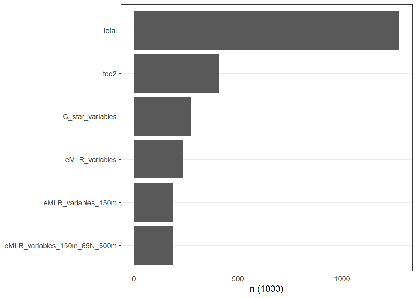
rm(GLODAP_stats_long)3.2 Assign coarse spatial grid
For the following plots, the cleaned data set was re-opened and observations were gridded spatially to intervals of:
- 5° x 5°
GLODAP <- read_csv(here::here("data/GLODAPv2_2020/_summarized_data_files",
                              "GLODAPv2.2020_clean.csv"))
GLODAP <- GLODAP %>%
mutate(lat_grid = cut(lat, seq(-90, 90, 5), seq(-87.5, 87.5, 5)),
lat_grid = as.numeric(as.character(lat_grid)),
lon_grid = cut(lon, seq(20, 380, 5), seq(22.5, 377.5, 5)),
lon_grid = as.numeric(as.character(lon_grid))) %>%
arrange(date)3.3 Histogram Zonal coverage
GLODAP_histogram_lat <- GLODAP %>%
  group_by(era, lat_grid, basin) %>%
  tally() %>%
  ungroup()

GLODAP_histogram_lat %>%
  ggplot(aes(lat_grid, n, fill = era)) +
  geom_col() +
  scale_x_continuous(breaks = seq(-87.5,90,10)) +
  scale_fill_brewer(palette = "Dark2") +
  facet_wrap(~basin) +
  coord_flip(expand = 0) +
  theme(legend.position = "top",
        legend.title = element_blank())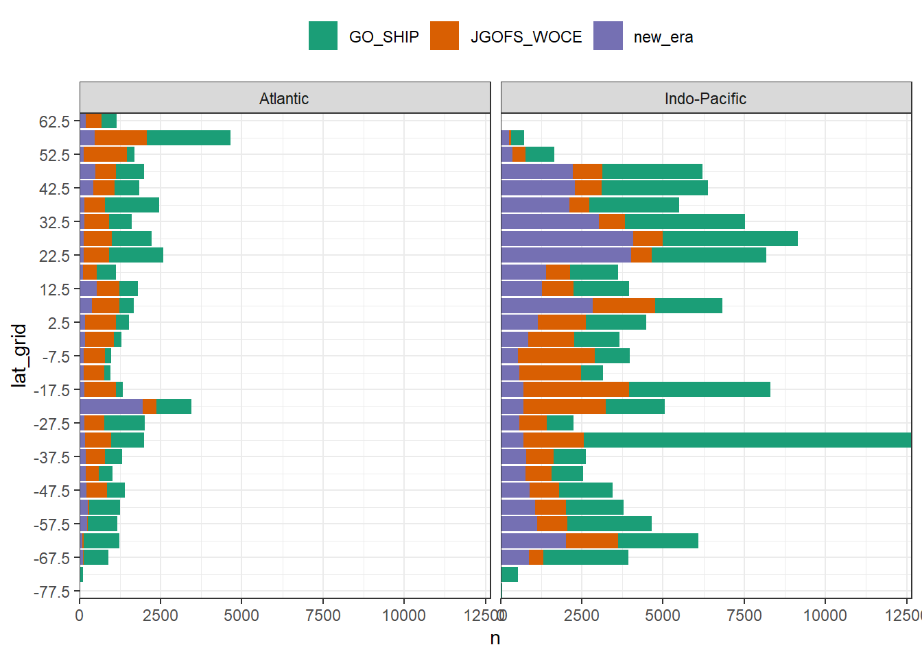
rm(GLODAP_histogram_lat)3.4 Histogram temporal coverage
GLODAP_histogram_year <- GLODAP %>%
  group_by(year, basin) %>%
  tally() %>%
  ungroup()

era_median_year <- GLODAP %>%
  group_by(era) %>%
  summarise(t_ref = median(year)) %>%
  ungroup()

GLODAP_histogram_year %>%
  ggplot() +
  geom_vline(xintercept = c(parameters$year_JGOFS_end + 0.5, parameters$year_GOSHIP_end + 0.5)) +
  geom_col(aes(year, n, fill = basin)) +
  geom_point(data = era_median_year, aes(t_ref,0, shape = "Median year"), size = 2, fill = "white") +
  scale_fill_brewer(palette = "Dark2") +
  scale_shape_manual(values = 24, name = "") +
  coord_cartesian(expand = 0) +
  theme(legend.position = "top",
        legend.direction = "vertical",
        legend.title = element_blank())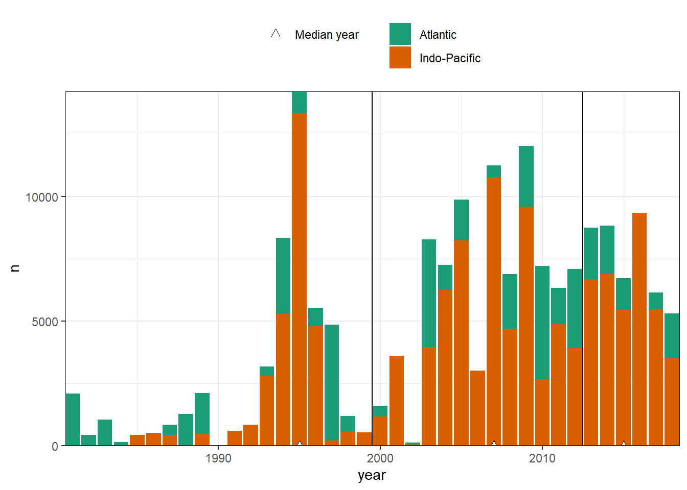
rm(GLODAP_histogram_year,
   era_median_year)
3.5 Zonal temporal coverage (Hovmoeller)
GLODAP_hovmoeller_year <- GLODAP %>%
  group_by(year, lat_grid, basin) %>%
  tally() %>%
  ungroup()

GLODAP_hovmoeller_year %>%
  ggplot(aes(year, lat_grid, fill = log10(n))) +
  geom_tile() +
  geom_vline(xintercept = c(1999.5, 2012.5)) +
  scale_fill_viridis_c(option = "magma", direction = -1) +
  facet_wrap(~basin, ncol = 1) +
  theme(legend.position = "top")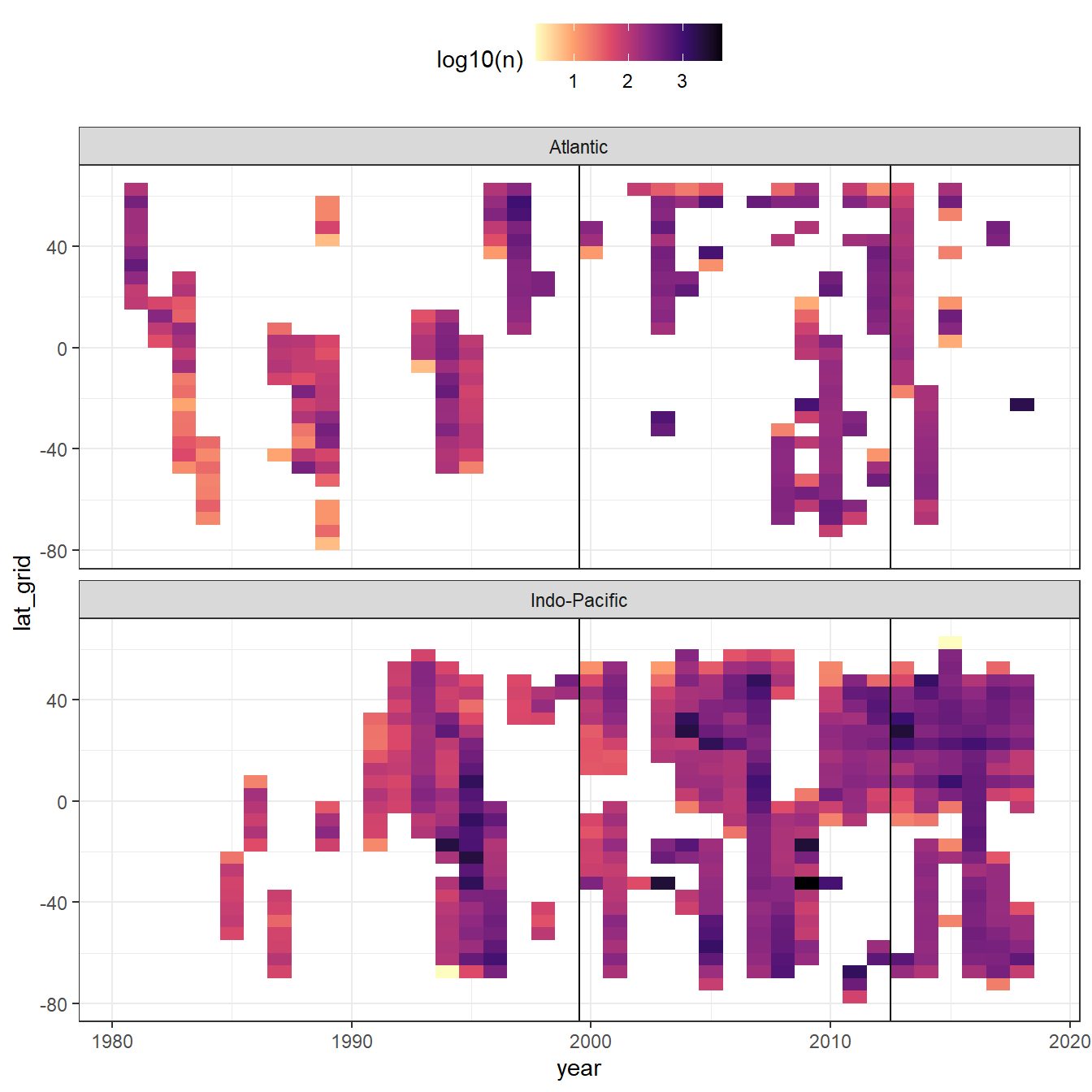
rm(GLODAP_hovmoeller_year)3.6 Coverage maps by era
GLODAP <- GLODAP %>%
  mutate(era = factor(era, c("JGOFS_WOCE", "GO_SHIP", "new_era")))

GLODAP %>%
  ggplot(aes(lon, lat)) +
  geom_raster(data = landmask %>% filter(region == "land"),
              aes(lon, lat), fill = "grey80") +
  geom_bin2d(binwidth = c(1,1)) +
  scale_fill_viridis_c(option = "magma", direction = -1, trans = "log10",
                       name = "log10(n)") +
  scale_x_continuous(breaks = seq(-180, 180, 30)) +
  scale_y_continuous(breaks = seq(-90, 90, 30)) +
  coord_quickmap(expand = FALSE) +
  facet_wrap(~era, ncol = 1) +
  theme(legend.position = "top")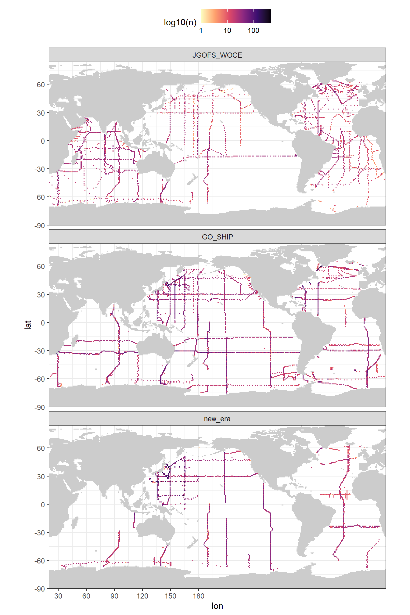
4 Individual cruise sections
Zonal and meridional section plots are produce for each cruise individually and can be downloaded here.
cruises <- GLODAP %>%
  group_by(cruise) %>%
  summarise(date_mean = mean(date, na.rm = TRUE),
            n = n()) %>%
  ungroup() %>%
  arrange(date_mean)

GLODAP <- full_join(GLODAP, cruises)

n <- 0
for (i_cruise in unique(cruises$cruise)) {

# i_cruise <- unique(cruises$cruise)[1]
n <- n+1
print(n)

GLODAP_cruise <- GLODAP %>%
  filter(cruise == i_cruise) %>%
  arrange(date)

cruises_cruise <- cruises %>%
  filter(cruise == i_cruise)

map <- GLODAP_cruise %>%
  ggplot(aes(lon, lat)) +
  geom_raster(data = landmask %>% filter(region == "land"),
              aes(lon, lat), fill = "grey80") +
  geom_point(aes(col=date)) +
  coord_quickmap(expand = FALSE) +
  scale_color_viridis_c(trans = "date") +
  labs(title = paste("Mean date:", cruises_cruise$date_mean,
                     "| cruise:", cruises_cruise$cruise,
                     "| n(samples):", cruises_cruise$n))


lon_section <- GLODAP_cruise %>%
  ggplot(aes(lon, depth)) +
  scale_y_reverse() +
  scale_color_viridis_c()

lon_tco2 <- lon_section+
  geom_point(aes(col=tco2))

lon_talk <- lon_section+
  geom_point(aes(col=talk))

lon_phosphate <- lon_section+
  geom_point(aes(col=phosphate))


lat_section <- GLODAP_cruise %>%
  ggplot(aes(lat, depth)) +
  scale_y_reverse() +
  scale_color_viridis_c()

lat_tco2 <- lat_section+
  geom_point(aes(col=tco2))

lat_talk <- lat_section+
  geom_point(aes(col=talk))

lat_phosphate <- lat_section+
  geom_point(aes(col=phosphate))

map /
((lat_tco2 / lat_talk / lat_phosphate) |
(lon_tco2 / lon_talk / lon_phosphate))

ggsave(here::here("output/figure/data/all_cruises_clean",
                  paste("GLODAP_cruise_date",
                        cruises_cruise$date_mean,
                        "n",
                        cruises_cruise$n,
                        "cruise",
                        cruises_cruise$cruise,
                        ".png",
                        sep = "_")),
                  width = 9, height = 9)

rm(map,
   lon_section, lat_section,
   lat_tco2, lat_talk, lat_phosphate, lon_tco2, lon_talk, lon_phosphate,
   GLODAP_cruise, cruises_cruise)

}
# library("rnaturalearth")
# library("rnaturalearthdata")
# library("sf")
#
# world <- ne_countries(scale = "small", returnclass = "sf")
# class(world)
#
# GLODAP_map <- GLODAP %>%
# group_by(lat_grid, lon_grid) %>%
# tally() %>%
# ungroup()
#
# ggplot() +
# geom_raster(data = GLODAP_map, aes(lon_grid, lat_grid)) +
# geom_sf(data = world) +
# coord_sf(crs = "+proj=robin +lat_0=0 +lon_0=0 +x0=0 +y0=0")
# https://gist.github.com/clauswilke/783e1a8ee3233775c9c3b8bfe531e28a
# https://twitter.com/clauswilke/status/1066024436208406529
# https://www.r-spatial.org/r/2018/10/25/ggplot2-sf.html5 Open tasks
- move A16 cruises in 2013 from new_era to GO_SHIP era
6 Questions
- Apply coastal filter?
- Keep horizontal gridding to 1°x1° (thereby discarding some horizontal information)?
- Quality of WOA18 basin mask
- excluded areas (e.g. Bay of Bengal, South Norwegian Sea, Sea of Japan)
- Pacific-Atlantic boundary
sessionInfo()R version 4.0.2 (2020-06-22)
Platform: x86_64-w64-mingw32/x64 (64-bit)
Running under: Windows 10 x64 (build 18363)
Matrix products: default
locale:
[1] LC_COLLATE=English_Germany.1252 LC_CTYPE=English_Germany.1252
[3] LC_MONETARY=English_Germany.1252 LC_NUMERIC=C
[5] LC_TIME=English_Germany.1252
attached base packages:
[1] stats graphics grDevices utils datasets methods base
other attached packages:
[1] patchwork_1.0.1 lubridate_1.7.9 forcats_0.5.0 stringr_1.4.0
[5] dplyr_1.0.0 purrr_0.3.4 readr_1.3.1 tidyr_1.1.0
[9] tibble_3.0.3 ggplot2_3.3.2 tidyverse_1.3.0 workflowr_1.6.2
loaded via a namespace (and not attached):
[1] Rcpp_1.0.5 here_0.1 assertthat_0.2.1 rprojroot_1.3-2
[5] digest_0.6.25 R6_2.4.1 cellranger_1.1.0 backports_1.1.8
[9] reprex_0.3.0 evaluate_0.14 httr_1.4.2 pillar_1.4.6
[13] rlang_0.4.7 readxl_1.3.1 rstudioapi_0.11 whisker_0.4
[17] blob_1.2.1 rmarkdown_2.3 labeling_0.3 munsell_0.5.0
[21] broom_0.7.0 compiler_4.0.2 httpuv_1.5.4 modelr_0.1.8
[25] xfun_0.16 pkgconfig_2.0.3 htmltools_0.5.0 tidyselect_1.1.0
[29] fansi_0.4.1 viridisLite_0.3.0 crayon_1.3.4 dbplyr_1.4.4
[33] withr_2.2.0 later_1.1.0.1 grid_4.0.2 jsonlite_1.7.0
[37] gtable_0.3.0 lifecycle_0.2.0 DBI_1.1.0 git2r_0.27.1
[41] magrittr_1.5 scales_1.1.1 cli_2.0.2 stringi_1.4.6
[45] farver_2.0.3 fs_1.4.2 promises_1.1.1 xml2_1.3.2
[49] ellipsis_0.3.1 generics_0.0.2 vctrs_0.3.2 RColorBrewer_1.1-2
[53] tools_4.0.2 glue_1.4.1 hms_0.5.3 yaml_2.2.1
[57] colorspace_1.4-1 rvest_0.3.6 knitr_1.29 haven_2.3.1