Prepare nitrate data and vertically align to same depths as (pH) climatology

workflowr

• Summary
• Checks
• Past versions

Last updated: 2023-12-06

Checks: 7 0

Knit directory: bgc_argo_r_argodata/

This reproducible R Markdown analysis was created with workflowr (version 1.7.0). The Checks tab describes the reproducibility checks that were applied when the results were created. The Past versions tab lists the development history.

---

R Markdown file: up-to-date

Great! Since the R Markdown file has been committed to the Git repository, you know the exact version of the code that produced these results.

Environment: empty

Great job! The global environment was empty. Objects defined in the global environment can affect the analysis in your R Markdown file in unknown ways. For reproduciblity it’s best to always run the code in an empty environment.

Seed: set.seed(20211008)

The command set.seed(20211008) was run prior to running the code in the R Markdown file. Setting a seed ensures that any results that rely on randomness, e.g. subsampling or permutations, are reproducible.

Session information: recorded

Great job! Recording the operating system, R version, and package versions is critical for reproducibility.

Cache: none

Nice! There were no cached chunks for this analysis, so you can be confident that you successfully produced the results during this run.

File paths: relative

Great job! Using relative paths to the files within your workflowr project makes it easier to run your code on other machines.

Repository version: 83269d5

Great! You are using Git for version control. Tracking code development and connecting the code version to the results is critical for reproducibility.

The results in this page were generated with repository version 83269d5. See the Past versions tab to see a history of the changes made to the R Markdown and HTML files.

Note that you need to be careful to ensure that all relevant files for the analysis have been committed to Git prior to generating the results (you can use wflow_publish or wflow_git_commit). workflowr only checks the R Markdown file, but you know if there are other scripts or data files that it depends on. Below is the status of the Git repository when the results were generated:

Ignored files:
    Ignored:    .Rhistory
    Ignored:    .Rproj.user/
    Ignored:    output/

Note that any generated files, e.g. HTML, png, CSS, etc., are not included in this status report because it is ok for generated content to have uncommitted changes.

---

These are the previous versions of the repository in which changes were made to the R Markdown (analysis/nitrate_vertical_align.Rmd) and HTML (docs/nitrate_vertical_align.html) files. If you’ve configured a remote Git repository (see ?wflow_git_remote), click on the hyperlinks in the table below to view the files as they were in that past version.

File	Version	Author	Date	Message
html	80c16c2	ds2n19	2023-11-15	Build site.
Rmd	3eba518	ds2n19	2023-11-15	Introduction of vertical alignment and cluster analysis to github website.

---

Task

This markdown file reads previously created pH climatology file and uses that as the definition of the depth levels that the Argo nitrate concentration data should be aligned to. Previously created BGC data (bgc_data.rds) and metadata (bgc_metadata.rds) are loaded from the BGC preprocessed folder.

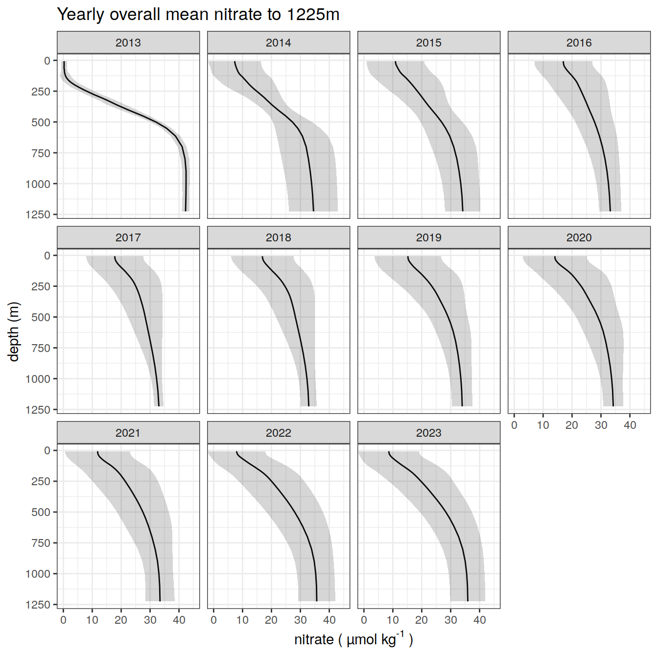
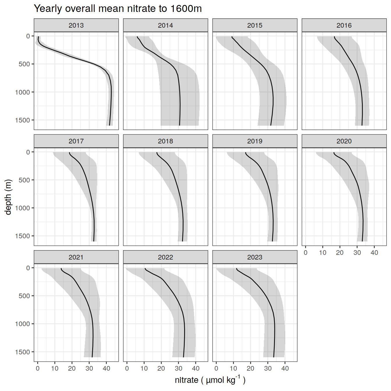
Base data qc flags are checked to ensure that the float position, pressure measurements and nitrate concentration measurements are good. Pressure is used to derive the depth of each measurement. The nitrate profile is checked to ensure that significant gaps (specified by the opt_gap_limit, opt_gap_min_depth and opt_gap_max_depth) do not exist. Profiles are assigned a profile_range field that identifies the depth 1 = 614 m, 2 = 1225 m and 3 = 1600 m.

The float nitrate profiles are then aligned using the spline function to match the depth levels of the climatology resulting in data frame bgc_data_nitrate_interpolated_clean.

Set directories

location of pre-prepared data

Set options

Define options that are used to determine profiles that we will us in the ongoing analysis

# Options

# opt_profile_depth_range
# The profile must have at least one nitrate reading at a depth <= opt_profile_depth_range[1, ]
# The profile must have at least one nitrate reading at a depth >= opt_profile_depth_range[2, ].
# In addition if the profile depth does not exceed the min(opt_profile_depth_range[2, ]) (i.e. 600) it will be removed.
profile_range <- c(1, 2, 3)
min_depth <- c(10, 10, 10)
max_depth <- c(614, 1225, 1600)
opt_profile_depth_range <- data.frame(profile_range, min_depth, max_depth)

# opt_gap...
# The profile should not have a gap greater that opt_gap_limit within the range defined by opt_gap_min_depth and opt_gap_max_depth
opt_gap_limit <- c(28, 55, 110)
opt_gap_min_depth <- c(0, 400, 1000)
opt_gap_max_depth <- c(400, 1000, 1600)

# opt_measure_label, opt_xlim and opt_xbreaks are associated formatting
opt_measure_label <- expression("nitrate ( µmol kg"^"-1"~")")
opt_xlim <- c(0, 45)
opt_xbreaks <- c(0, 10, 20, 30, 40)

# opt_n_prof_sel
# The selection criteria that is used against n_prof, here set to 1
# Description of n_prof usage is provided at https://argo.ucsd.edu/data/data-faq/version-3-profile-files/ the next two lines are from that page.
#     The main Argo CTD profile is stored in N_PROF=1. All other parameters (including biogeochemical parameters) that are measured 
#     with the same vertical sampling scheme and at the same location and time as the main Argo CTD profile are also stored in N_PROF=1.
opt_n_prof_sel = 1

read climatology

read pH climatology, values are provided at set depths

# climatology values (pH_clim_va) available for lat, lon, month and depth
pH_clim_va <- read_rds(file = paste0(path_argo_preprocessed, "/pH_clim_va.rds"))

# What is the max depth we are interested in
opt_profile_max_depth <- max(opt_profile_depth_range$max_depth)

# existing depth levels that we will align to
target_depth_levels <-   pH_clim_va %>%
  filter(depth <= opt_profile_max_depth) %>%
  rename(target_depth = depth) %>%
  distinct(target_depth)

rm(pH_clim_va)
gc()

          used (Mb) gc trigger  (Mb) max used  (Mb)
Ncells 1276526 68.2    2476592 132.3  2476592 132.3
Vcells 2192581 16.8   91951966 701.6 92803109 708.1

read nitrate data

read nitrate profile and carry out basic checks, good data.

# base data and associated metadata
bgc_data <- read_rds(file = paste0(path_argo_preprocessed, '/bgc_data.rds'))
bgc_metadata <- read_rds(file = paste0(path_argo_preprocessed, '/bgc_metadata.rds'))

# Select relevant field from metadata ready to join to bgc_data
bgc_metadata_select <- bgc_metadata %>%
  filter(position_qc == 1) %>%
  select(file_id,
         date,
         lat,
         lon) %>%
  mutate(year = year(date),
         month = month(date),
         .after = date)

# we drive alignment from pressure and nitrate data
# conditions 
# n_prof == 1
# pres_adjusted_qc %in% c(1, 8) - pressure data marked as good
# nitrate_adjusted_qc %in% c(1, 8) - nitrate data marked as good
# !is.na(pres_adjusted) - pressure value must be present
# !is.na(nitrate_adjusted) - nitrate value must be present
bgc_data_nitrate <- bgc_data %>%
  filter(
    pres_adjusted_qc %in% c(1, 8) &
      nitrate_adjusted_qc %in% c(1, 8) &
      n_prof == opt_n_prof_sel &
      !is.na(pres_adjusted) &
      !is.na(nitrate_adjusted)
  ) %>%
  select(file_id,
         pres_adjusted,
         nitrate_adjusted)

# join with metadata information and calculate depth field
bgc_data_nitrate <- inner_join(bgc_metadata_select %>% select(file_id, lat),
                          bgc_data_nitrate) %>%
  mutate(depth = gsw_z_from_p(pres_adjusted, latitude = lat) * -1.0,
         .before = pres_adjusted) %>%
  select(-c(lat, pres_adjusted))

# ensure we have a depth, and nitrate_adjusted for all rows in bgc_data_nitrate
bgc_data_nitrate <- bgc_data_nitrate %>%
                  filter(!is.na(depth) & !is.na(nitrate_adjusted))

# clean up working tables
rm(bgc_data, bgc_metadata)
gc()

          used (Mb) gc trigger    (Mb)   max used    (Mb)
Ncells 1313126 70.2    2476592   132.3    2476592   132.3
Vcells 9590565 73.2 2796663182 21336.9 3467835783 26457.5

Profile limits

Apply the rules that are determined by options set in set_options. Profile must cover a set range and not contain gaps.

# Determine profile min and max depths
bgc_profile_limits <- bgc_data_nitrate %>%
  group_by(file_id) %>%
  summarise(
    min_depth = min(depth),
    max_depth = max(depth),
  ) %>%
  ungroup()

# The profile much match at least one of the range criteria
force_min <- min(opt_profile_depth_range$min_depth)
force_max <- min(opt_profile_depth_range$max_depth)

# Apply profile min and max restrictions
bgc_apply_limits <- bgc_profile_limits %>%
  filter(
    min_depth <= force_min &
    max_depth >= force_max
    )

# Ensure working data set only contains profiles that have confrormed to the range test
bgc_data_nitrate <- right_join(bgc_data_nitrate,
                          bgc_apply_limits %>% select(file_id))


# Add profile type field and set all to 1.  
# All profile that meet the minimum requirements are profile_range = 1
bgc_data_nitrate <- bgc_data_nitrate %>%
  mutate(profile_range = 1)

for (i in 2:nrow(opt_profile_depth_range)) {

  #i = 3
  range_min <- opt_profile_depth_range[i,'min_depth']
  range_max <- opt_profile_depth_range[i,'max_depth']

  # Apply profile min and max restrictions
  bgc_apply_limits <- bgc_profile_limits %>%
    filter(min_depth <= range_min &
             max_depth >= range_max) %>%
    select(file_id) %>%
    mutate (profile_range = i)

  # Update profile range to i for these profiles
  # bgc_data_temp <- full_join(bgc_data_temp, bgc_apply_limits) %>%
  #                         filter(!is.na(min_depth))
  bgc_data_nitrate <-
    bgc_data_nitrate %>% rows_update(bgc_apply_limits, by = "file_id")
  
}

# Find the gaps within the profiles
profile_gaps <- full_join(bgc_data_nitrate,
                          opt_profile_depth_range) %>%
  filter(depth >= min_depth & 
           depth <= max_depth) %>% 
  select(file_id,
         depth) %>%
  arrange(file_id, depth) %>%
  group_by(file_id) %>%
  mutate(gap = depth - lag(depth, default = 0)) %>%
  ungroup()

# Ensure we do not have gaps in the profile that invalidate it 
for (i_gap in opt_gap_limit) {

  # The limits to be applied in that pass of for loop
  # i_gap <- opt_gap_limit[3]
  i_gap_min = opt_gap_min_depth[which(opt_gap_limit == i_gap)]
  i_gap_max = opt_gap_max_depth[which(opt_gap_limit == i_gap)]
  
  # Which gaps are greater than i_gap
  profile_gaps_remove <- profile_gaps %>%
    filter(gap > i_gap) %>%
    filter(depth >= i_gap_min & depth <= i_gap_max) %>%
    distinct(file_id) %>% 
    pull()
  
  # Remonve these profiles from working data set
  bgc_data_nitrate <- bgc_data_nitrate %>% 
    filter(!file_id %in% profile_gaps_remove)

}

# clean up working tables
rm(bgc_profile_limits, profile_gaps, profile_gaps_remove, bgc_apply_limits)
gc()

           used (Mb) gc trigger    (Mb)   max used    (Mb)
Ncells  1328168 71.0    2476592   132.3    2476592   132.3
Vcells 10141670 77.4 2237330546 17069.5 3467835783 26457.5

Vertical align nitrate

We have a set of nitrate profiles that match our criteria we now need to align that data set to match the depth that are in target_depth_range, this will match the range of climatology values in ucsd_clim

# create unique combinations of file_id and profile ranges
profile_range_file_id <- 
  bgc_data_nitrate %>% 
  distinct(file_id, profile_range)


# select variable of interest and prepare target_depth field
bgc_data_nitrate_clean <- bgc_data_nitrate %>%
  select(-profile_range) %>%
  mutate(target_depth = depth, .after = depth)

rm(bgc_data_nitrate)
gc()

          used (Mb) gc trigger    (Mb)   max used    (Mb)
Ncells 1327923 71.0    2476592   132.3    2476592   132.3
Vcells 8200935 62.6 1789864437 13655.6 3467835783 26457.5

# create all possible combinations of location, month and depth levels for interpolation
target_depth_grid <-
  expand_grid(
    target_depth_levels,
    profile_range_file_id
  )

# Constrain target_depth_grid to profile depth range
target_depth_grid <-
  left_join(target_depth_grid, opt_profile_depth_range) %>%
  filter(target_depth <= max_depth)

target_depth_grid <- target_depth_grid %>%
  select(target_depth,
         file_id)

# extend nitrate depth vectors with target depths
bgc_data_nitrate_extended <-
  full_join(bgc_data_nitrate_clean, target_depth_grid) %>%
  arrange(file_id, target_depth)

rm(bgc_data_nitrate_clean)
gc()

           used  (Mb) gc trigger    (Mb)   max used    (Mb)
Ncells  1330239  71.1    2476592   132.3    2476592   132.3
Vcells 15642402 119.4 1431891550 10924.5 3467835783 26457.5

# predict spline interpolation on adjusted depth grid for nitrate location and month
bgc_data_nitrate_interpolated <-
  bgc_data_nitrate_extended %>%
  group_by(file_id) %>%
  mutate(nitrate_spline = spline(target_depth, nitrate_adjusted,
                                method = "natural",
                                xout = target_depth)$y) %>%
  ungroup()

rm(bgc_data_nitrate_extended)
gc()

           used  (Mb) gc trigger   (Mb)   max used    (Mb)
Ncells  1332014  71.2    2476592  132.3    2476592   132.3
Vcells 18721328 142.9 1145513240 8739.6 3467835783 26457.5

# subset interpolated values on target depth range
bgc_data_nitrate_interpolated_clean <- 
  inner_join(target_depth_levels, bgc_data_nitrate_interpolated)

rm(bgc_data_nitrate_interpolated)
gc()

          used (Mb) gc trigger   (Mb)   max used    (Mb)
Ncells 1332058 71.2    2476592  132.3    2476592   132.3
Vcells 9793524 74.8  916410592 6991.7 3467835783 26457.5

# select columns and rename to initial names
bgc_data_nitrate_interpolated_clean <-
  bgc_data_nitrate_interpolated_clean %>%
  select(file_id,
         depth = target_depth,
         nitrate = nitrate_spline)

# merge with profile range
bgc_data_nitrate_interpolated_clean <-
  full_join(bgc_data_nitrate_interpolated_clean,
            profile_range_file_id)

# merge with meta data
bgc_data_nitrate_interpolated_clean <-
  left_join(bgc_data_nitrate_interpolated_clean,
            bgc_metadata_select)

Write files

Write the interpolated nitrate profiles that map onto depth levels.

# Write files
bgc_data_nitrate_interpolated_clean %>%
  write_rds(file = paste0(path_argo_preprocessed, "/nitrate_bgc_va.rds"))

# Rename so that names match if just reading existing files
nitrate_bgc_va <- bgc_data_nitrate_interpolated_clean

rm(bgc_data_nitrate_interpolated_clean)
gc()

           used  (Mb) gc trigger   (Mb)   max used    (Mb)
Ncells  1331859  71.2    2476592  132.3    2476592   132.3
Vcells 14154178 108.0  733128474 5593.4 3467835783 26457.5

read files

Read files that were previously created ready for analysis

# read files
nitrate_bgc_va <- read_rds(file = paste0(path_argo_preprocessed, "/nitrate_bgc_va.rds"))

Analysis

nitrate mean profile

max_depth_1 <- opt_profile_depth_range[1, "max_depth"]
max_depth_2 <- opt_profile_depth_range[2, "max_depth"]
max_depth_3 <- opt_profile_depth_range[3, "max_depth"]

# Profiles to 600m
nitrate_overall_mean_1 <- nitrate_bgc_va %>% 
  filter(profile_range %in% c(1, 2, 3) & depth <= max_depth_1) %>%
  group_by(depth) %>% 
  summarise(count_measures = n(),
            nitrate_mean = mean(nitrate, na.rm = TRUE),
            nitrate_sd = sd(nitrate, na.rm = TRUE))

nitrate_year_mean_1 <- nitrate_bgc_va %>% 
  filter(profile_range %in% c(1, 2, 3) & depth <= max_depth_1) %>%
  group_by(year, depth) %>% 
  summarise(count_measures = n(),
            nitrate_mean = mean(nitrate, na.rm = TRUE),
            nitrate_sd = sd(nitrate, na.rm = TRUE))

# Profiles to 1200m
nitrate_overall_mean_2 <- nitrate_bgc_va %>% 
  filter(profile_range %in% c(2, 3) & depth <= max_depth_2) %>%
  group_by(depth) %>% 
  summarise(count_measures = n(),
            nitrate_mean = mean(nitrate, na.rm = TRUE),
            nitrate_sd = sd(nitrate, na.rm = TRUE))

nitrate_year_mean_2 <- nitrate_bgc_va %>% 
  filter(profile_range %in% c(2, 3) & depth <= max_depth_2) %>%
  group_by(year, depth) %>% 
  summarise(count_measures = n(),
            nitrate_mean = mean(nitrate, na.rm = TRUE),
            nitrate_sd = sd(nitrate, na.rm = TRUE))

# Profiles to 1500m
nitrate_overall_mean_3 <- nitrate_bgc_va %>% 
  filter(profile_range %in% c(3) & depth <= max_depth_3) %>%
  group_by(depth) %>% 
  summarise(count_measures = n(),
            nitrate_mean = mean(nitrate, na.rm = TRUE),
            nitrate_sd = sd(nitrate, na.rm = TRUE))

nitrate_year_mean_3 <- nitrate_bgc_va %>% 
  filter(profile_range %in% c(3) & depth <= max_depth_3) %>%
  group_by(year, depth) %>% 
  summarise(count_measures = n(),
            nitrate_mean = mean(nitrate, na.rm = TRUE),
            nitrate_sd = sd(nitrate, na.rm = TRUE))

# All years
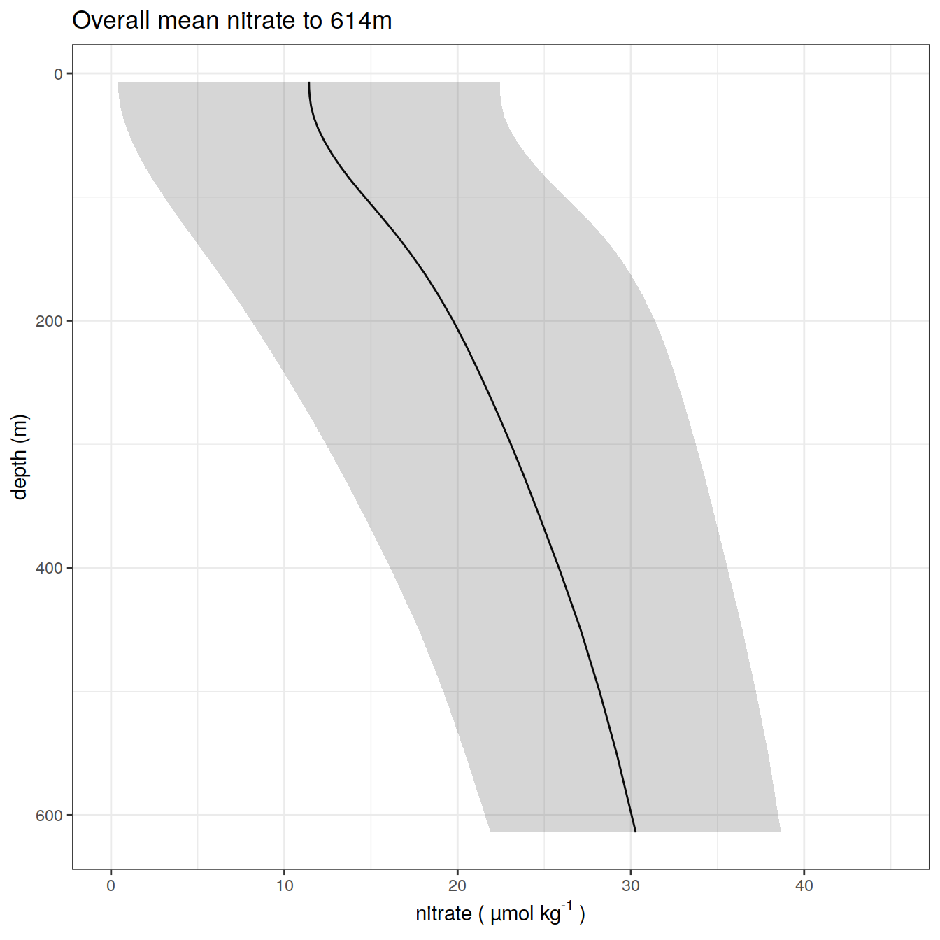
nitrate_overall_mean_1 %>% 
  ggplot()+
  geom_path(aes(x = nitrate_mean,
                y = depth))+
  geom_ribbon(aes(
    xmax = nitrate_mean + nitrate_sd,
    xmin = nitrate_mean - nitrate_sd,
    y = depth
  ),
  alpha = 0.2) +
  scale_y_reverse()+
  coord_cartesian(xlim = opt_xlim)+
  scale_x_continuous(breaks = opt_xbreaks)+
  labs(
    title = paste0('Overall mean nitrate to ', max_depth_1, 'm'), 
    x=opt_measure_label, 
    y='depth (m)'
  )

Past versions of plot_overall_mean_nitrate_profiles-1.png

Version	Author	Date
80c16c2	ds2n19	2023-11-15

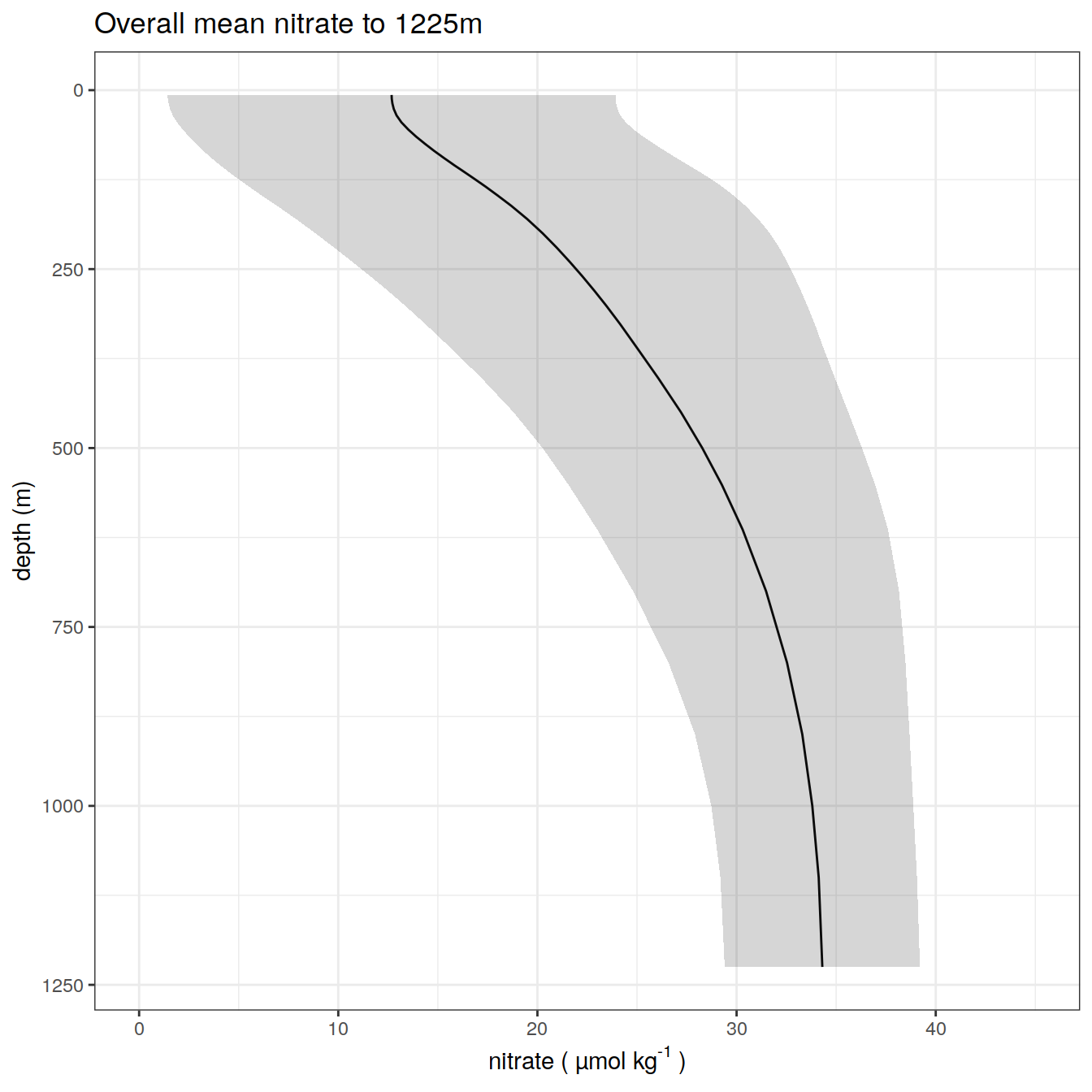
nitrate_overall_mean_2 %>% 
  ggplot()+
  geom_path(aes(x = nitrate_mean,
                y = depth))+
  geom_ribbon(aes(
    xmax = nitrate_mean + nitrate_sd,
    xmin = nitrate_mean - nitrate_sd,
    y = depth
  ),
  alpha = 0.2) +
  scale_y_reverse()+
  coord_cartesian(xlim = opt_xlim)+
  scale_x_continuous(breaks = opt_xbreaks)+
  labs(
    title = paste0('Overall mean nitrate to ', max_depth_2, 'm'), 
    x=opt_measure_label, 
    y='depth (m)'
  )

Past versions of plot_overall_mean_nitrate_profiles-2.png

Version	Author	Date
80c16c2	ds2n19	2023-11-15

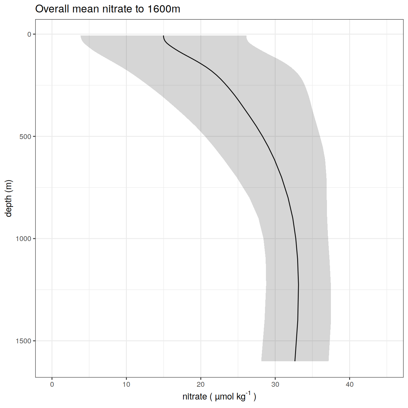
nitrate_overall_mean_3 %>% 
  ggplot()+
  geom_path(aes(x = nitrate_mean,
                y = depth))+
  geom_ribbon(aes(
    xmax = nitrate_mean + nitrate_sd,
    xmin = nitrate_mean - nitrate_sd,
    y = depth
  ),
  alpha = 0.2) +
  scale_y_reverse()+
  coord_cartesian(xlim = opt_xlim)+
  scale_x_continuous(breaks = opt_xbreaks)+
  labs(
    title = paste0('Overall mean nitrate to ', max_depth_3, 'm'), 
    x=opt_measure_label, 
    y='depth (m)'
  )

Past versions of plot_overall_mean_nitrate_profiles-3.png

Version	Author	Date
80c16c2	ds2n19	2023-11-15

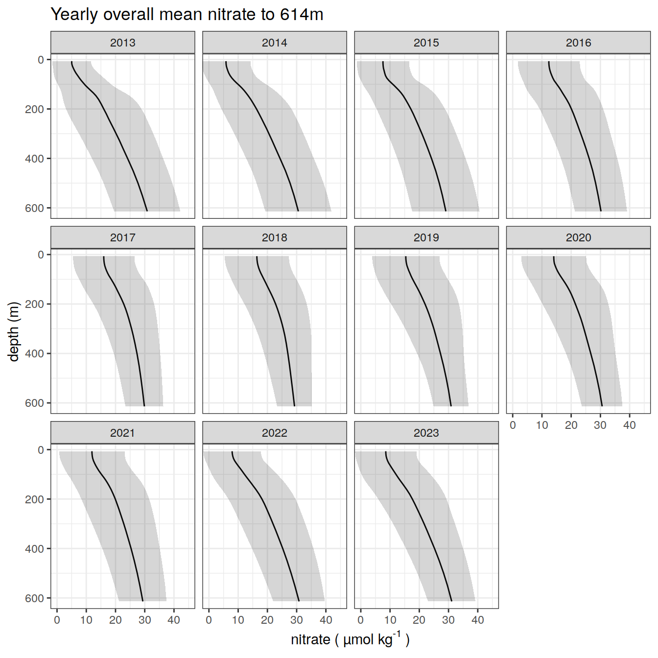
# by years
nitrate_year_mean_1 %>% 
  ggplot()+
  geom_path(aes(x = nitrate_mean,
                y = depth))+
  geom_ribbon(aes(
    xmax = nitrate_mean + nitrate_sd,
    xmin = nitrate_mean - nitrate_sd,
    y = depth
  ),
  alpha = 0.2) +
  scale_y_reverse()+
  facet_wrap(~year)+
  coord_cartesian(xlim = opt_xlim)+
  scale_x_continuous(breaks = opt_xbreaks)+
  labs(
    title = paste0('Yearly overall mean nitrate to ', max_depth_1, 'm'),
    x = opt_measure_label,
    y = 'depth (m)'
  )

Past versions of plot_overall_mean_nitrate_profiles-4.png

Version	Author	Date
80c16c2	ds2n19	2023-11-15

nitrate_year_mean_2 %>% 
  ggplot()+
  geom_path(aes(x = nitrate_mean,
                y = depth))+
  geom_ribbon(aes(
    xmax = nitrate_mean + nitrate_sd,
    xmin = nitrate_mean - nitrate_sd,
    y = depth
  ),
  alpha = 0.2) +
  scale_y_reverse()+
  facet_wrap(~year)+
  coord_cartesian(xlim = opt_xlim)+
  scale_x_continuous(breaks = opt_xbreaks)+
  labs(
    title = paste0('Yearly overall mean nitrate to ', max_depth_2, 'm'),
    x = opt_measure_label,
    y = 'depth (m)'
  )

Past versions of plot_overall_mean_nitrate_profiles-5.png

Version	Author	Date
80c16c2	ds2n19	2023-11-15

nitrate_year_mean_3 %>% 
  ggplot()+
  geom_path(aes(x = nitrate_mean,
                y = depth))+
  geom_ribbon(aes(
    xmax = nitrate_mean + nitrate_sd,
    xmin = nitrate_mean - nitrate_sd,
    y = depth
  ),
  alpha = 0.2) +
  scale_y_reverse()+
  facet_wrap(~year)+
  coord_cartesian(xlim = opt_xlim)+
  scale_x_continuous(breaks = opt_xbreaks)+
  labs(
    title = paste0('Yearly overall mean nitrate to ', max_depth_3, 'm'),
    x = opt_measure_label,
    y = 'depth (m)'
  )

Past versions of plot_overall_mean_nitrate_profiles-6.png

Version	Author	Date
80c16c2	ds2n19	2023-11-15

Profile counts

Details of the number of profiles and to which depths over the analysis period

nitrate_histogram <- nitrate_bgc_va %>%
  group_by(year, profile_range = as.character(profile_range)) %>%
  summarise(num_profiles = n_distinct(file_id)) %>%
  ungroup()

nitrate_histogram %>%
  ggplot() +
  geom_bar(
    aes(
      x = year,
      y = num_profiles,
      fill = profile_range,
      group = profile_range
    ),
    position = "stack",
    stat = "identity"
  ) +
  scale_fill_viridis_d() +
  labs(title = "nitrate profiles per year and profile range",
       x = "year",
       y = "profile count",
       fill = "profile range")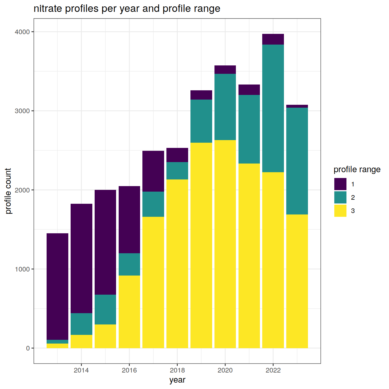

Past versions of nitrate_histogram-1.png

Version	Author	Date
80c16c2	ds2n19	2023-11-15

Session information

sessionInfo()

R version 4.2.2 (2022-10-31)
Platform: x86_64-pc-linux-gnu (64-bit)
Running under: openSUSE Leap 15.5

Matrix products: default
BLAS:   /usr/local/R-4.2.2/lib64/R/lib/libRblas.so
LAPACK: /usr/local/R-4.2.2/lib64/R/lib/libRlapack.so

locale:
 [1] LC_CTYPE=en_US.UTF-8       LC_NUMERIC=C              
 [3] LC_TIME=en_US.UTF-8        LC_COLLATE=en_US.UTF-8    
 [5] LC_MONETARY=en_US.UTF-8    LC_MESSAGES=en_US.UTF-8   
 [7] LC_PAPER=en_US.UTF-8       LC_NAME=C                 
 [9] LC_ADDRESS=C               LC_TELEPHONE=C            
[11] LC_MEASUREMENT=en_US.UTF-8 LC_IDENTIFICATION=C       

attached base packages:
[1] stats     graphics  grDevices utils     datasets  methods   base     

other attached packages:
 [1] gsw_1.1-1        gridExtra_2.3    lubridate_1.9.0  timechange_0.1.1
 [5] argodata_0.1.0   forcats_0.5.2    stringr_1.5.0    dplyr_1.1.3     
 [9] purrr_1.0.2      readr_2.1.3      tidyr_1.3.0      tibble_3.2.1    
[13] ggplot2_3.4.4    tidyverse_1.3.2 

loaded via a namespace (and not attached):
 [1] Rcpp_1.0.10         assertthat_0.2.1    rprojroot_2.0.3    
 [4] digest_0.6.30       utf8_1.2.2          R6_2.5.1           
 [7] cellranger_1.1.0    backports_1.4.1     reprex_2.0.2       
[10] evaluate_0.18       highr_0.9           httr_1.4.4         
[13] pillar_1.9.0        rlang_1.1.1         googlesheets4_1.0.1
[16] readxl_1.4.1        rstudioapi_0.15.0   whisker_0.4        
[19] jquerylib_0.1.4     rmarkdown_2.18      labeling_0.4.2     
[22] googledrive_2.0.0   munsell_0.5.0       broom_1.0.5        
[25] compiler_4.2.2      httpuv_1.6.6        modelr_0.1.10      
[28] xfun_0.35           pkgconfig_2.0.3     htmltools_0.5.3    
[31] tidyselect_1.2.0    workflowr_1.7.0     viridisLite_0.4.1  
[34] fansi_1.0.3         crayon_1.5.2        withr_2.5.0        
[37] tzdb_0.3.0          dbplyr_2.2.1        later_1.3.0        
[40] grid_4.2.2          jsonlite_1.8.3      gtable_0.3.1       
[43] lifecycle_1.0.3     DBI_1.1.3           git2r_0.30.1       
[46] magrittr_2.0.3      scales_1.2.1        cli_3.6.1          
[49] stringi_1.7.8       cachem_1.0.6        farver_2.1.1       
[52] fs_1.5.2            promises_1.2.0.1    xml2_1.3.3         
[55] bslib_0.4.1         ellipsis_0.3.2      generics_0.1.3     
[58] vctrs_0.6.4         tools_4.2.2         glue_1.6.2         
[61] RNetCDF_2.6-1       hms_1.1.2           fastmap_1.1.0      
[64] yaml_2.3.6          colorspace_2.0-3    gargle_1.2.1       
[67] rvest_1.0.3         knitr_1.41          haven_2.5.1        
[70] sass_0.4.4