Extreme pH Profiles
Pasqualina Vonlanthen, David Stappard & Jens Daniel Müller
14 May, 2024
Last updated: 2024-05-14
Checks: 7 0
Knit directory:
bgc_argo_r_argodata/analysis/
This reproducible R Markdown analysis was created with workflowr (version 1.7.0). The Checks tab describes the reproducibility checks that were applied when the results were created. The Past versions tab lists the development history.
Great! Since the R Markdown file has been committed to the Git repository, you know the exact version of the code that produced these results.
Great job! The global environment was empty. Objects defined in the global environment can affect the analysis in your R Markdown file in unknown ways. For reproduciblity it’s best to always run the code in an empty environment.
The command set.seed(20211008) was run prior to running
the code in the R Markdown file. Setting a seed ensures that any results
that rely on randomness, e.g. subsampling or permutations, are
reproducible.
Great job! Recording the operating system, R version, and package versions is critical for reproducibility.
Nice! There were no cached chunks for this analysis, so you can be confident that you successfully produced the results during this run.
Great job! Using relative paths to the files within your workflowr project makes it easier to run your code on other machines.
Great! You are using Git for version control. Tracking code development and connecting the code version to the results is critical for reproducibility.
The results in this page were generated with repository version 91e6028. See the Past versions tab to see a history of the changes made to the R Markdown and HTML files.
Note that you need to be careful to ensure that all relevant files for
the analysis have been committed to Git prior to generating the results
(you can use wflow_publish or
wflow_git_commit). workflowr only checks the R Markdown
file, but you know if there are other scripts or data files that it
depends on. Below is the status of the Git repository when the results
were generated:
Ignored files:
    Ignored:    .Rproj.user/

Untracked files:
    Untracked:  analysis/draft.Rmd
    Untracked:  load_argo_core_output.txt

Unstaged changes:
    Deleted:    analysis/MHWs_categorisation.Rmd
    Modified:   analysis/_site.yml
    Modified:   analysis/child/cluster_analysis_base.Rmd
    Modified:   analysis/coverage_maps_North_Atlantic.Rmd
    Modified:   analysis/load_broullon_DIC_TA_clim.Rmd
    Modified:   code/Workflowr_project_managment.R
    Modified:   code/start_background_job.R
    Modified:   code/start_background_job_load.R
    Modified:   code/start_background_job_partial.R
Note that any generated files, e.g. HTML, png, CSS, etc., are not included in this status report because it is ok for generated content to have uncommitted changes.
These are the previous versions of the repository in which changes were
made to the R Markdown (analysis/extreme_compound.Rmd) and
HTML (docs/extreme_compound.html) files. If you’ve
configured a remote Git repository (see ?wflow_git_remote),
click on the hyperlinks in the table below to view the files as they
were in that past version.
| File | Version | Author | Date | Message |
|---|---|---|---|---|
| html | af6594f | mlarriere | 2024-05-13 | Build site. |
| html | af44bcd | mlarriere | 2024-04-26 | Build site. |
| html | 780276c | mlarriere | 2024-04-19 | Build site. |
| html | 1a72545 | mlarriere | 2024-04-12 | Build site. |
| html | c076fba | mlarriere | 2024-04-12 | Build site. |
| html | 91f08a6 | mlarriere | 2024-04-07 | Build site. |
| html | db21f55 | mlarriere | 2024-04-06 | Build site. |
| html | 488ff93 | mlarriere | 2024-04-01 | Build site. |
| html | f9de50e | ds2n19 | 2024-01-01 | Build site. |
| html | 07d4eb8 | ds2n19 | 2023-12-20 | Build site. |
| html | fa6cf38 | ds2n19 | 2023-12-14 | Build site. |
| Rmd | 64fd104 | ds2n19 | 2023-12-14 | revised coverage analysis and SO focused cluster analysis. |
| html | f110b74 | ds2n19 | 2023-12-13 | Build site. |
| Rmd | fa9795c | ds2n19 | 2023-12-12 | dependencies listed are start of markdown files. |
| html | e60ebd2 | ds2n19 | 2023-12-07 | Build site. |
| html | cf5dd20 | ds2n19 | 2023-12-04 | Build site. |
| Rmd | 3cb4b17 | ds2n19 | 2023-12-04 | Cluster under surface extreme. |
| Rmd | fa1083d | ds2n19 | 2023-12-01 | Additional analysis to cluster process. |
| html | cec2a2a | ds2n19 | 2023-11-24 | Build site. |
| Rmd | 3dc557d | ds2n19 | 2023-11-24 | Switched to new profile details. |
| Rmd | 59f5cc4 | ds2n19 | 2023-11-23 | Moved spatiotemporal analysis to use aligned profiles. |
| html | 80c16c2 | ds2n19 | 2023-11-15 | Build site. |
| html | 4b55c43 | ds2n19 | 2023-10-12 | Build site. |
| Rmd | ce19a66 | ds2n19 | 2023-10-04 | Revised version of OceanSODA product -v2023 |
| html | 7b3d8c5 | pasqualina-vonlanthendinenna | 2022-08-29 | Build site. |
| html | bdd516d | pasqualina-vonlanthendinenna | 2022-05-23 | Build site. |
| html | 4173c20 | jens-daniel-mueller | 2022-05-12 | Build site. |
| html | dfe89d7 | jens-daniel-mueller | 2022-05-12 | Build site. |
| html | 710edd4 | jens-daniel-mueller | 2022-05-11 | Build site. |
| Rmd | 2f20a76 | jens-daniel-mueller | 2022-05-11 | rebuild all after subsetting AB profiles and code cleaning |
Task
Explore double extremes in the temp and pH anomaly fields
Dependencies
pH_bgc_va.rds - bgc preprocessed folder, created by ph_align_climatology.
temp_bgc_va.rds - bgc preprocessed folder, created by temp_align_climatology.
OceanSODA_pH_anomaly_field_01.rds (or _02.rds) - bgc preprocessed folder, extreme_pH
OceanSODA_SST_anomaly_field_01.rds (or _02.rds) - bgc preprocessed folder, extreme_temp
Load Data
library(tidyverse)
library(lubridate)
library(ggnewscale)
theme_set(theme_bw())
HNL_colors_map <- c('H' = 'red3',
'N' = 'gray90',
'L' = 'blue3')
# opt_min_profile_range
# profiles with profile_range >= opt_min_profile_range will be selected
# 1 = profiles of at least pH = 614m temp = 600m, 2 = profiles of at least pH = 1225m temp = 1200m, 3 = profiles of at least pH = 1600m temp = 1500m
opt_min_profile_range = 3
# opt_extreme_determination
# 1 - based on the trend of de-seasonal data - we believe this results in more summer extremes where variation tend to be greater.
# 2 - based on the trend of de-seasonal data by month. grouping is by lat, lon and month.
opt_extreme_determination <- 2path_argo <- '/nfs/kryo/work/updata/bgc_argo_r_argodata'
path_argo_preprocessed <- paste0(path_argo, "/preprocessed_bgc_data")
path_emlr_utilities <- "/nfs/kryo/work/jenmueller/emlr_cant/utilities/files/"
path_argo <- '/nfs/kryo/work/datasets/ungridded/3d/ocean/floats/bgc_argo'
# /nfs/kryo/work/datasets/ungridded/3d/ocean/floats/bgc_argo/preprocessed_bgc_data
path_argo_preprocessed <- paste0(path_argo, "/preprocessed_bgc_data")map <-
read_rds(paste(path_emlr_utilities,
"map_landmask_WOA18.rds",
sep = ""))
if (opt_extreme_determination == 1){
pH_extreme <- read_rds(file = paste0(path_argo_preprocessed, "/OceanSODA_pH_anomaly_field_01.rds"))
temp_extreme <- read_rds(file = paste0(path_argo_preprocessed, "/OceanSODA_SST_anomaly_field_01.rds"))
} else if (opt_extreme_determination == 2){
pH_extreme <- read_rds(file = paste0(path_argo_preprocessed, "/OceanSODA_pH_anomaly_field_02.rds"))
temp_extreme <- read_rds(file = paste0(path_argo_preprocessed, "/OceanSODA_SST_anomaly_field_02.rds"))
}
# load validated and vertically aligned pH profiles,
argo_pH <- read_rds(file = paste0(path_argo_preprocessed, "/pH_bgc_va.rds")) %>%
filter(profile_range >= opt_min_profile_range) %>%
select(file_id,
date,
year,
month,
lat,
lon,
depth,
profile_range_pH = profile_range,
pH,
h_plus)
argo_temp <- read_rds(file = paste0(path_argo_preprocessed, "/temp_bgc_va.rds")) %>%
filter(profile_range >= opt_min_profile_range) %>%
select(file_id,
date,
year,
month,
lat,
lon,
depth,
profile_range_temp = profile_range,
temp)
full_argo <- full_join(argo_pH, argo_temp)
# list where both pH and temp exist and apply to full_argo
argo_file_id <- inner_join(argo_pH %>% distinct(file_id), argo_temp %>% distinct(file_id))
full_argo <- left_join(argo_file_id, full_argo)
# change the date format for compatibility with OceanSODA pH data
full_argo <- full_argo %>%
mutate(date = ymd(format(date, "%Y-%m-15")))
rm(argo_pH, argo_temp, argo_file_id)Anomaly maps
pH
pH_extreme %>%
  filter(year >= 2013) %>%
  group_split(month) %>%
  #head(1) %>%
  map(
    ~map +
      geom_tile(data = .x,
                aes(x = lon_raw,
                    y = lat_raw,
                    fill = ph_extreme))+
      scale_fill_manual(values = HNL_colors_map)+
      facet_wrap(~year, ncol = 2)+
      lims(y = c(-85, -32))+
      labs(title = paste('month:', unique(.x$month)),
           fill = 'pH')
  )
[[1]]
[[2]]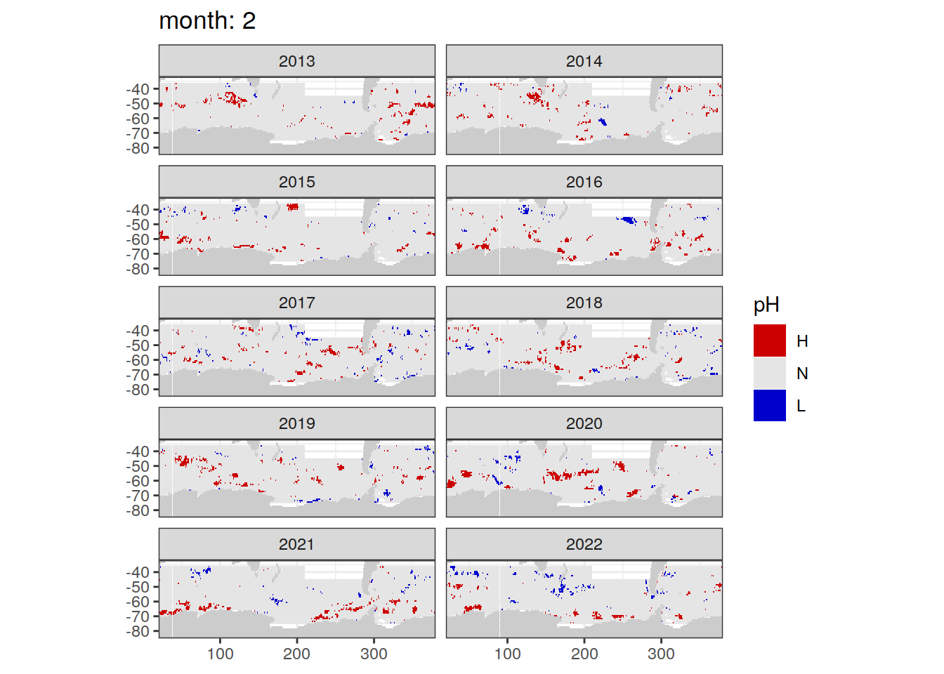
[[3]]
[[4]]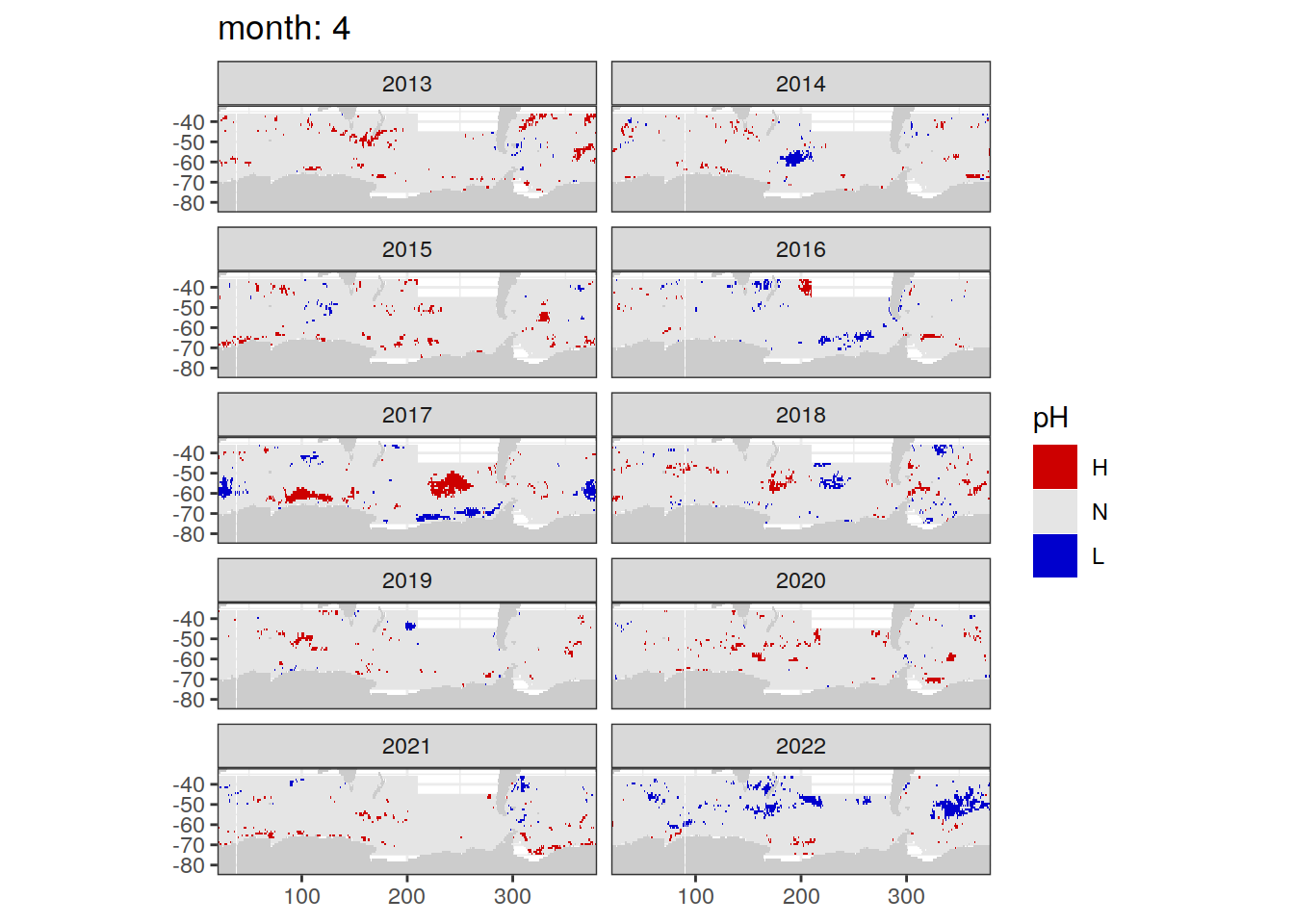
[[5]]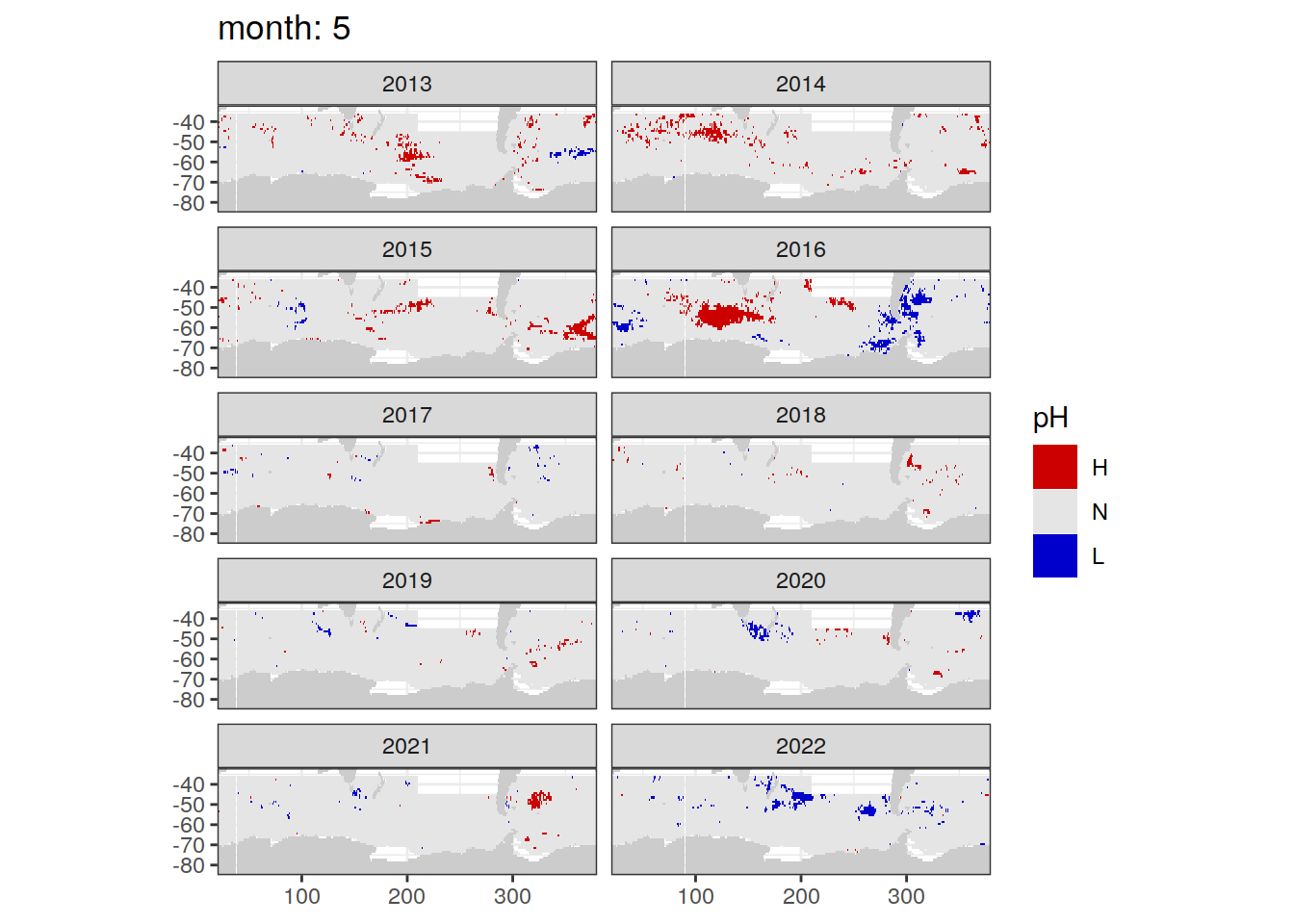
[[6]]
[[7]]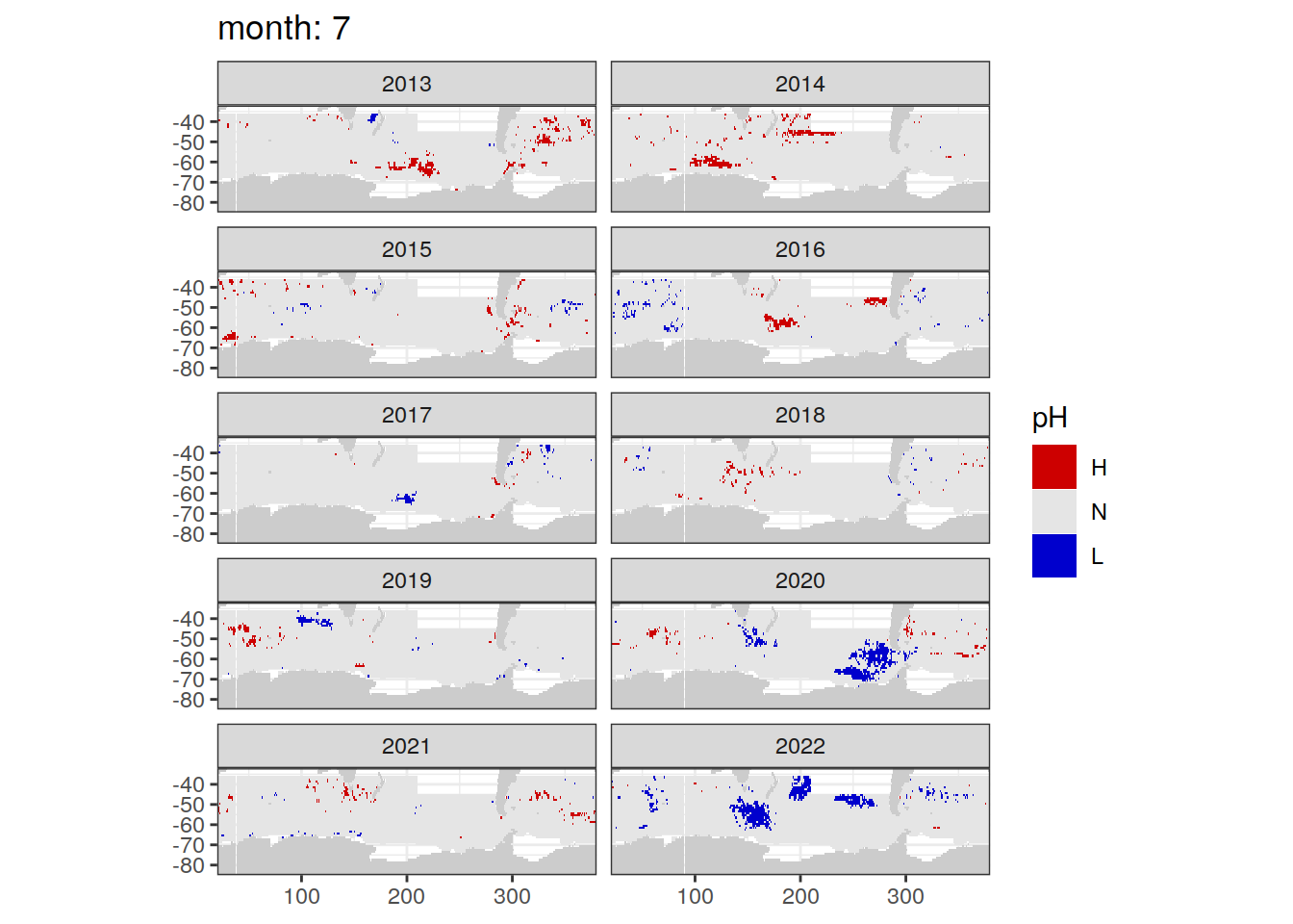
[[8]]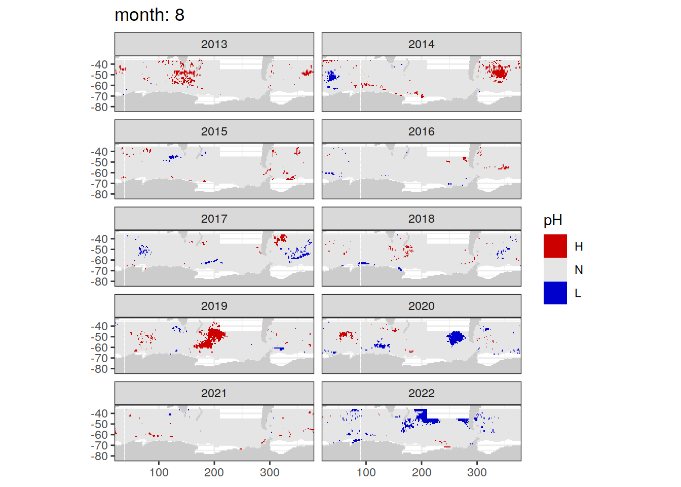
[[9]]
[[10]]
[[11]]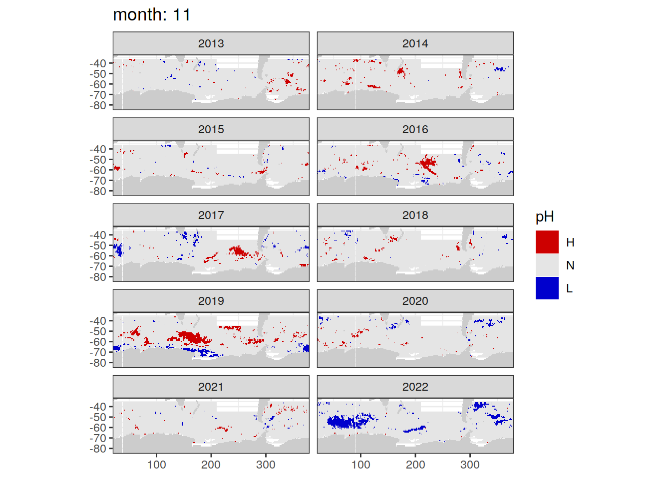
[[12]]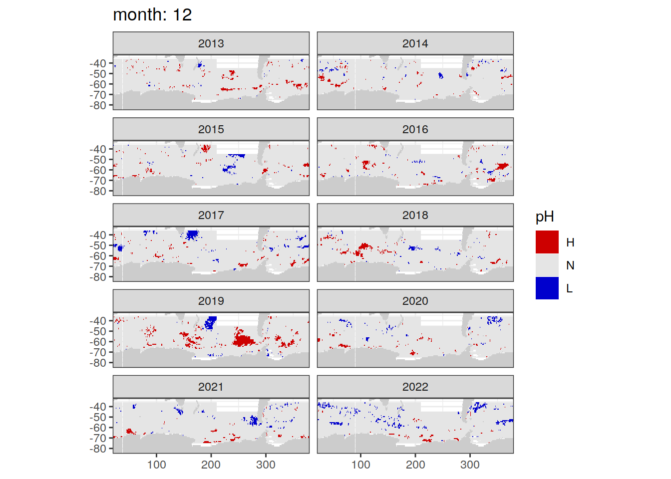
SST
temp_extreme %>%
  filter(year >= 2013) %>%
  group_split(month) %>%
  #head(1) %>%
  map(
    ~map +
      geom_tile(data = .x,
                aes(x = lon_raw,
                    y = lat_raw,
                    fill = temp_extreme))+
      scale_fill_manual(values = HNL_colors_map)+
      facet_wrap(~year, ncol = 2)+
      lims(y = c(-85, -32))+
      labs(title = paste('month:', unique(.x$month)),
           fill = 'pH')
  )
[[1]]
[[2]]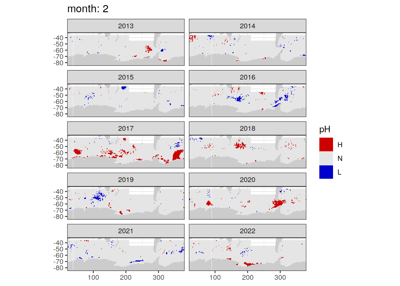
[[3]]
[[4]]
[[5]]
[[6]]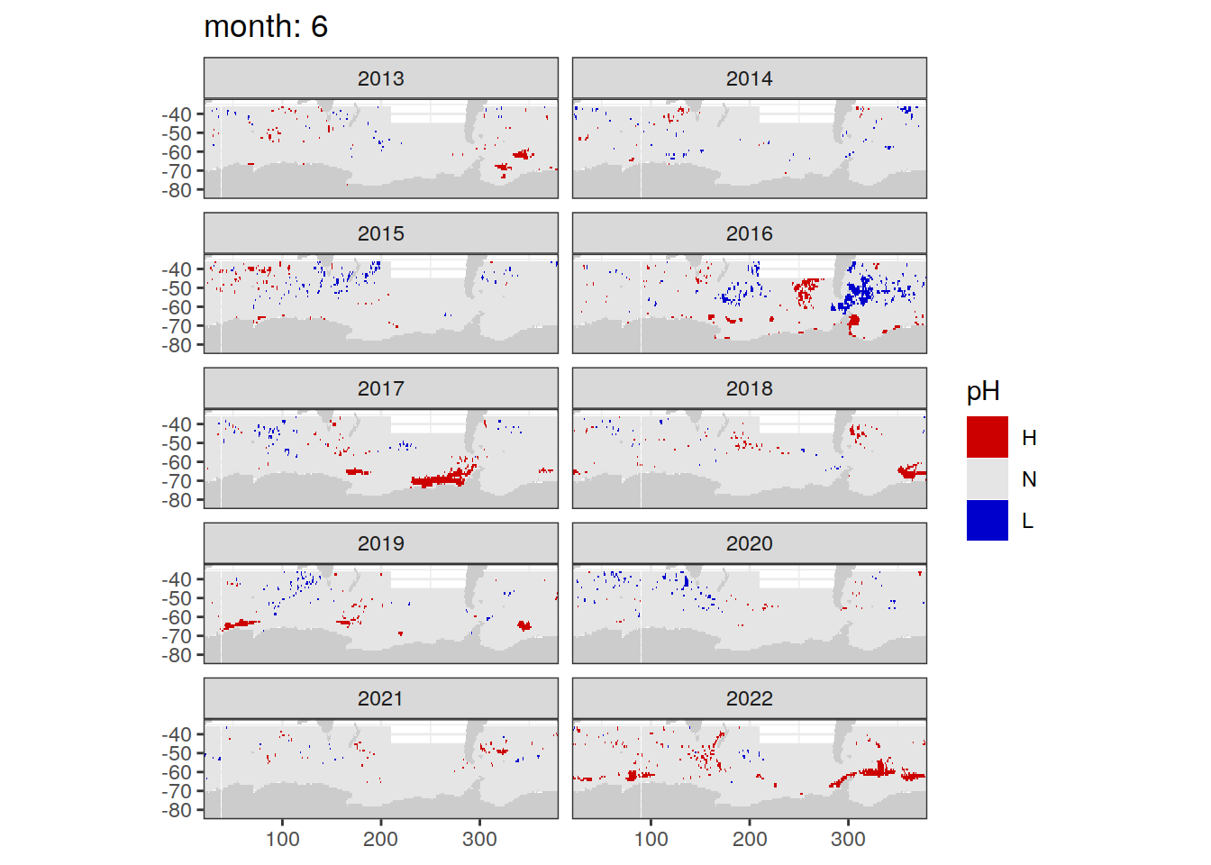
[[7]]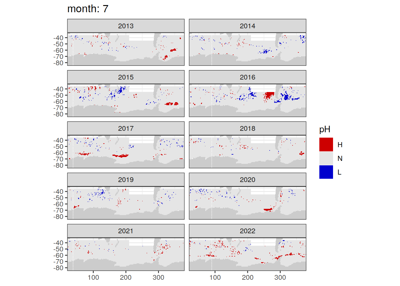
[[8]]
[[9]]
[[10]]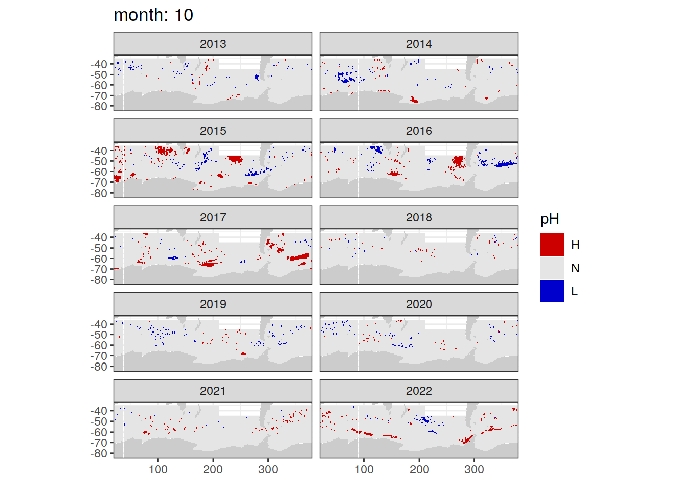
[[11]]
[[12]]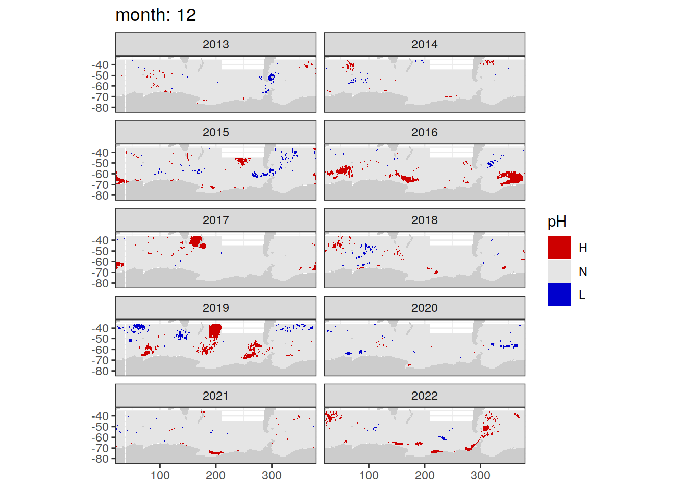
Join data
anomaly_field <- full_join(pH_extreme %>%
                             select(lon_raw, lat_raw, month, year, date, basin_AIP, biome_name, ph_extreme),
                           temp_extreme %>%
                             select(lon_raw, lat_raw, month, year, date, basin_AIP, biome_name, temp_extreme))
# chisq.test(anomaly_field$ph_extreme, anomaly_field$temp_extreme, correct = FALSE)
anomaly_field <- anomaly_field %>%
mutate(
double_extreme = case_when(
temp_extreme == 'H' & ph_extreme == 'H' ~ 'warm_HpH',
temp_extreme == 'L' &
ph_extreme == 'H' ~ 'cold_HpH',
temp_extreme == 'H' &
ph_extreme == 'L' ~ 'warm_LpH',
temp_extreme == 'L' &
ph_extreme == 'L' ~ 'cold_LpH',
temp_extreme == 'H' &
ph_extreme == 'N' ~ 'warm',
temp_extreme == 'L' &
ph_extreme == 'N' ~ 'cold',
temp_extreme == 'N' &
ph_extreme == 'H' ~ 'HpH',
temp_extreme == 'N' &
ph_extreme == 'L' ~ 'LpH',
TRUE ~ 'N'
)
) %>%
mutate(
double_extreme = fct_relevel(
double_extreme,
'warm_HpH',
'cold_HpH',
'warm_LpH',
'cold_LpH',
'warm',
'cold',
'HpH',
'LpH',
'N'
)
)Compound extreme maps
HNL_colors_map_temp <- c('H' = "#CD534CFF",
                    'N' = 'transparent',
                    'L' = "#0073C2FF")

HNL_colors_map_ph <- c('H' = "#009E73",
                    'N' = 'transparent',
                    'L' = "#EFC000FF")


anomaly_field %>%
  filter(year >= 2013,
         double_extreme != "N") %>%
  group_split(month) %>%
  # tail(1) %>%
  map(
    ~ map +
      geom_tile(data = .x,
                aes(
                  x = lon_raw,
                  y = lat_raw,
                  fill = ph_extreme
                ), alpha = 0.4) +
      scale_fill_manual(values = HNL_colors_map_ph) +
      new_scale_fill() +
      geom_tile(data = .x,
                aes(
                  x = lon_raw,
                  y = lat_raw,
                  fill = temp_extreme
                ), alpha = 0.4) +
      scale_fill_manual(values = HNL_colors_map_temp) +
      facet_wrap(~ year, ncol = 2) +
      lims(y = c(-85, -32)) +
      labs(title = paste0('month:', unique(.x$month)))
  )
[[1]]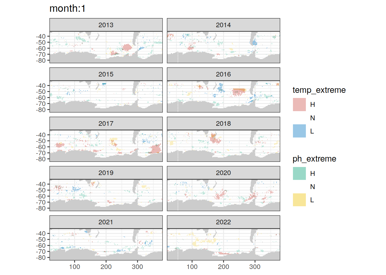
[[2]]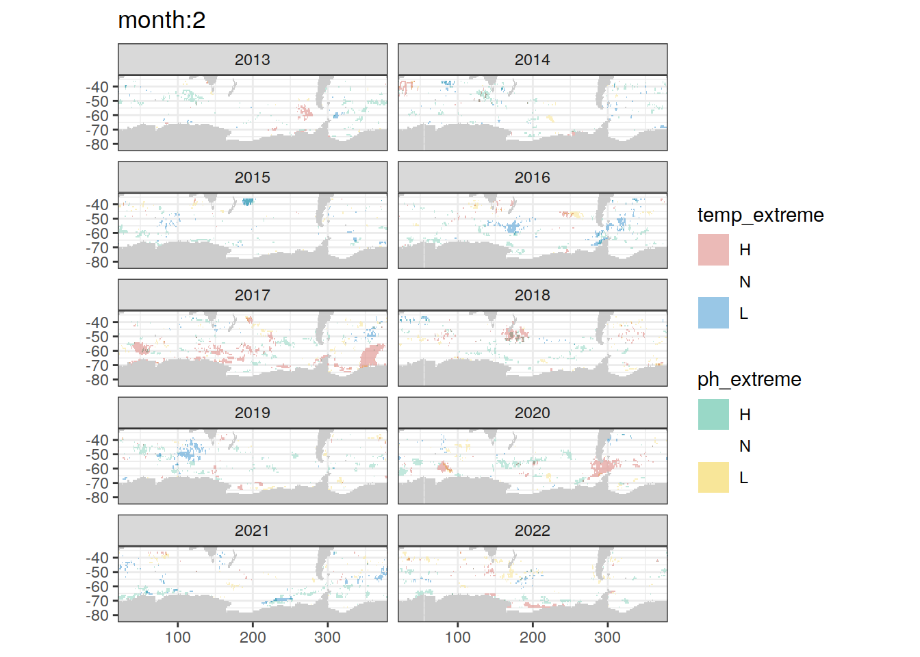
[[3]]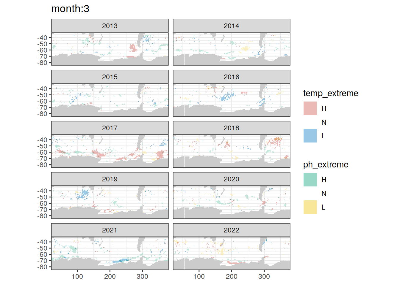
[[4]]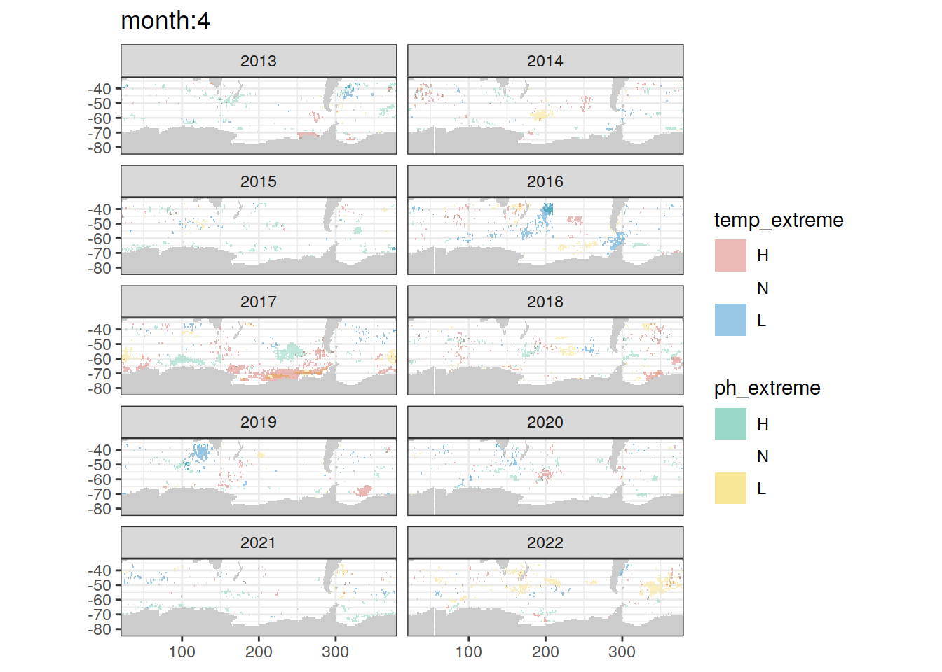
[[5]]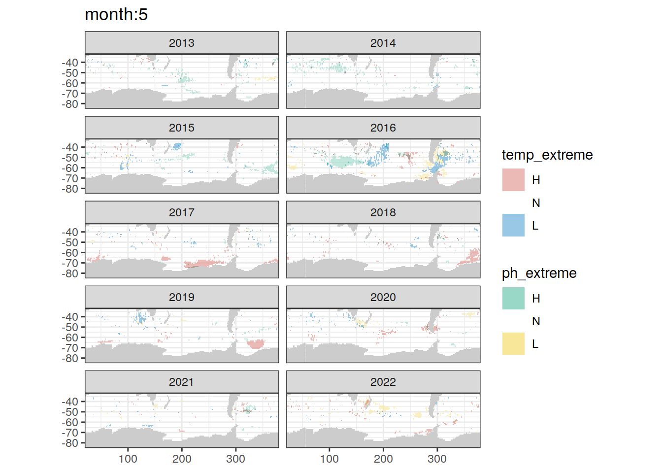
[[6]]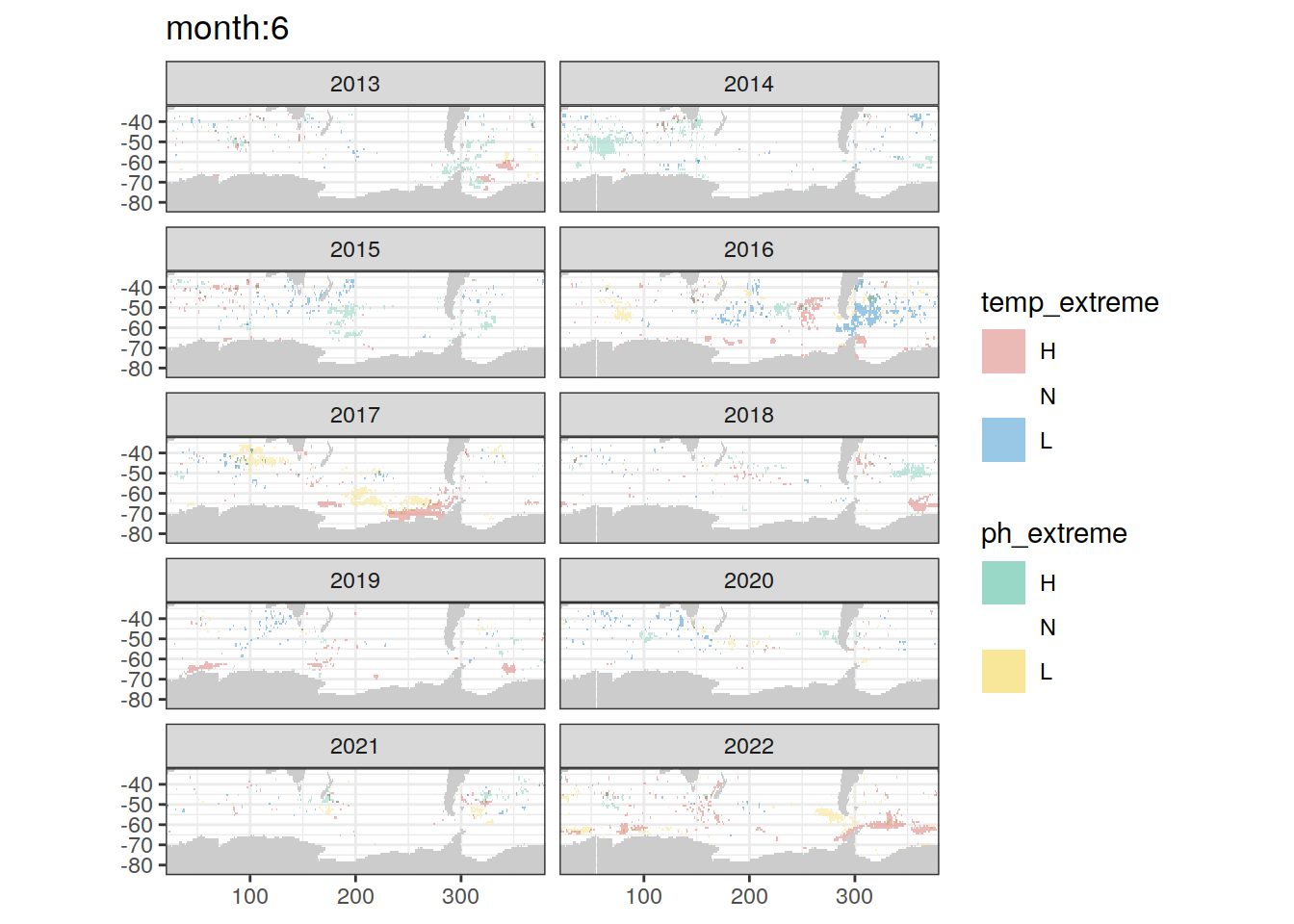
[[7]]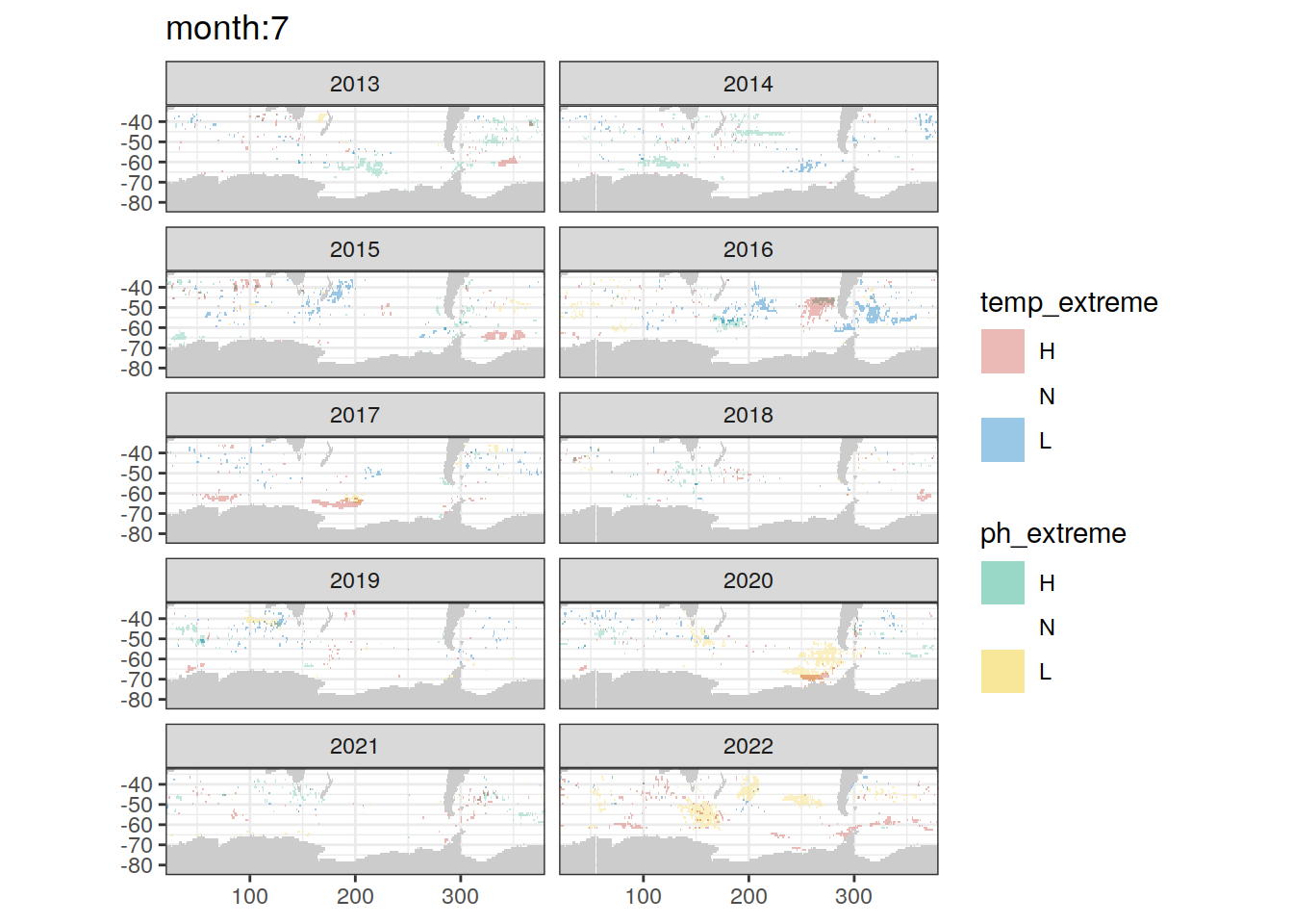
[[8]]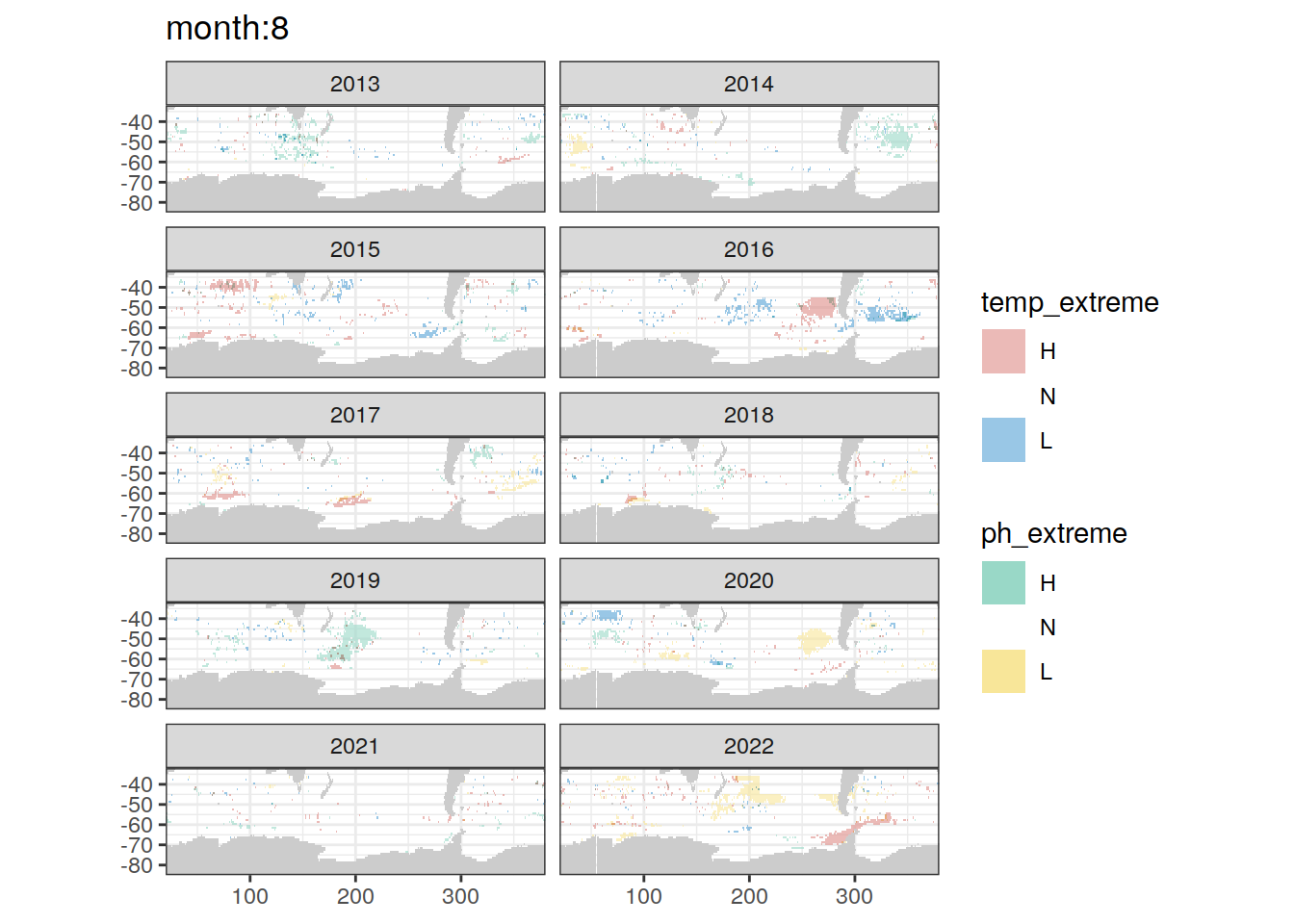
[[9]]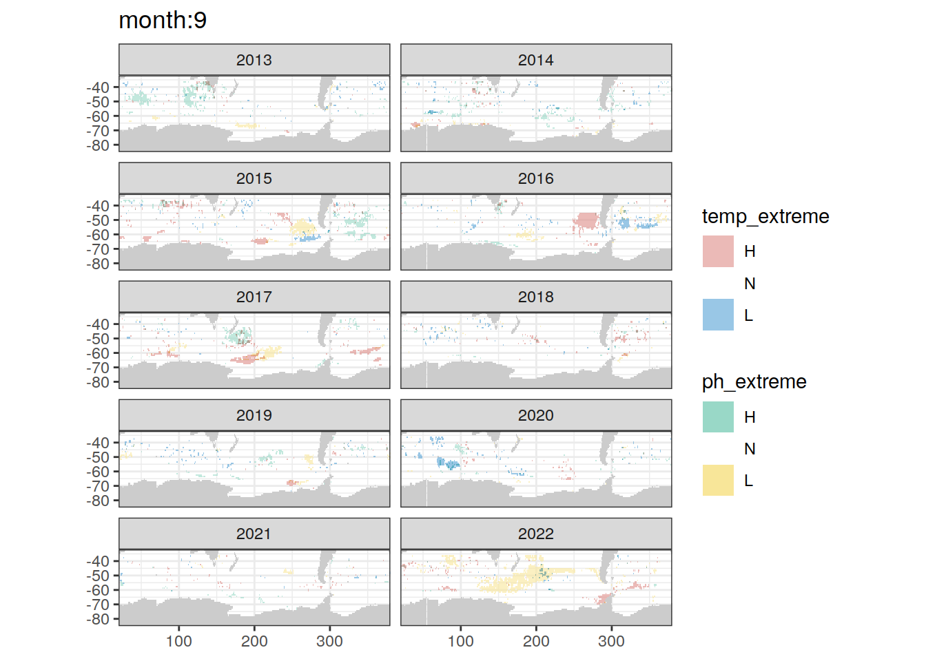
[[10]]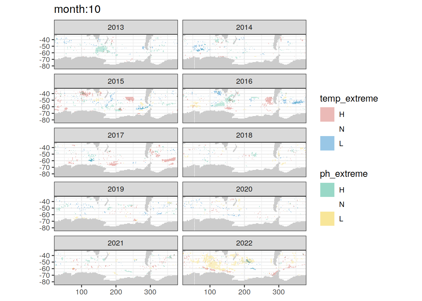
[[11]]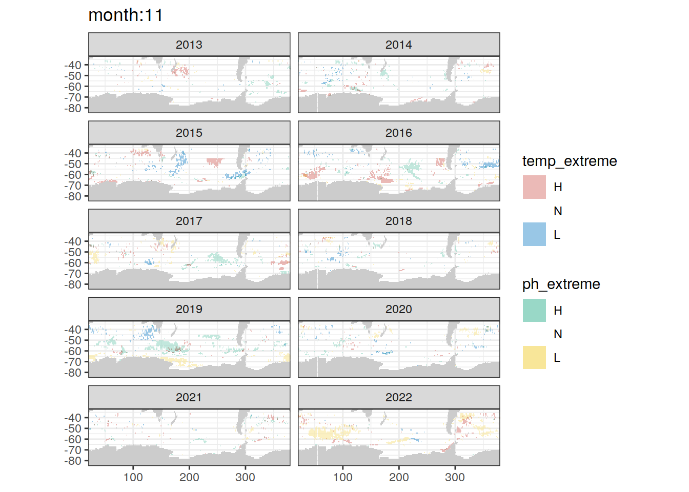
[[12]]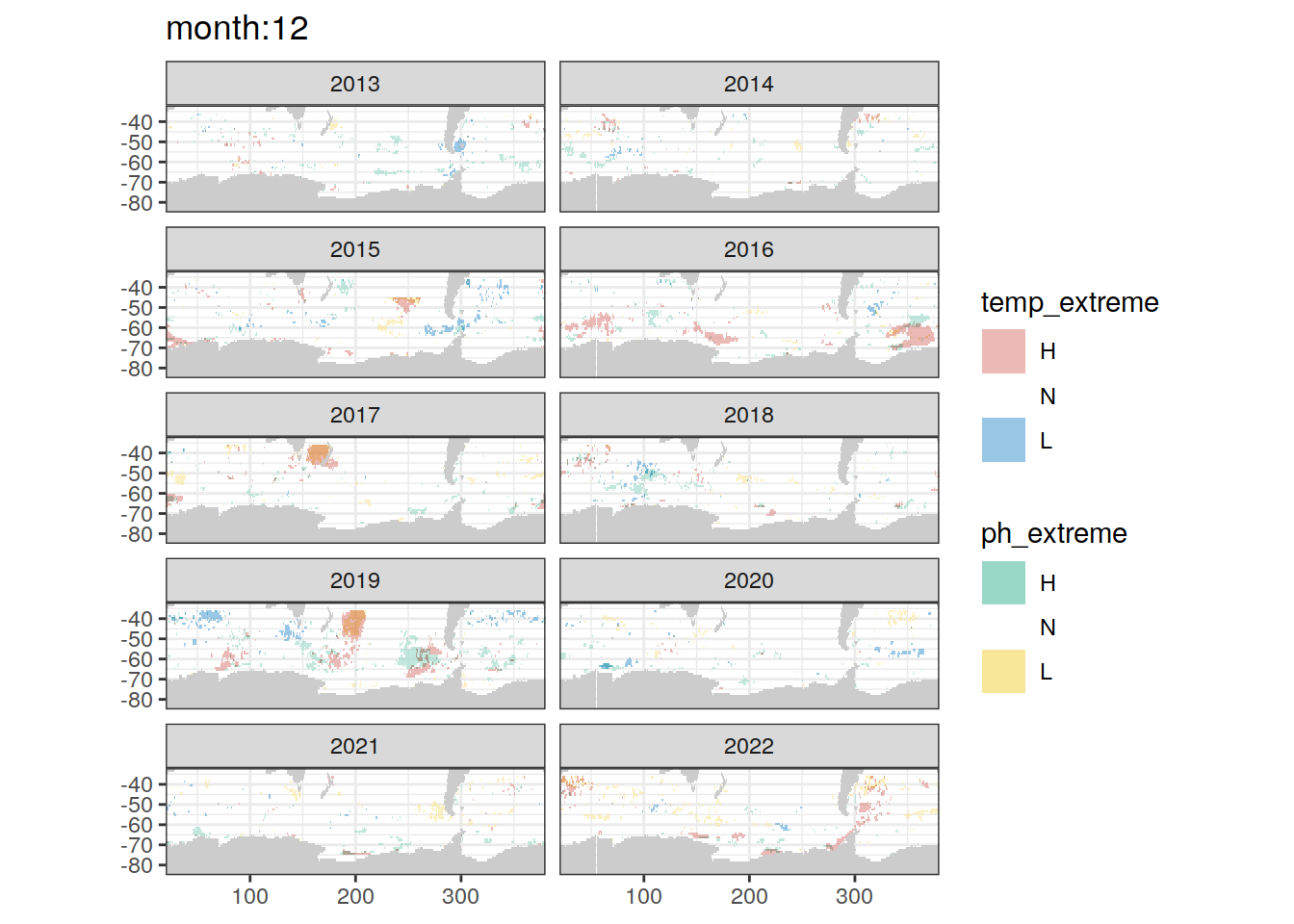
rm(HNL_colors_map_temp, HNL_colors_map_ph)anomaly_field %>%
filter(year >= 2013) %>%
group_split(month) %>%
map(
~map+
geom_tile(data = .x,
aes(x = lon_raw,
y = lat_raw,
fill = double_extreme))+
facet_wrap(~year, ncol = 2)+
scale_fill_manual(values = c('warm_HpH' = 'brown',
'warm_LpH' = 'yellow',
'cold_HpH' = 'beige',
'cold_LpH' = 'cyan',
'cold' = 'blue',
'warm' = 'red',
'LpH' = 'orange',
'HpH' = 'green',
'N' = NA),
na.value = NA)+
lims(y = c(-85, -32))+
labs(title = paste0('month:', unique(.x$month)),
fill = 'double extreme')
)[[1]]
[[2]]
[[3]]
[[4]]
[[5]]
[[6]]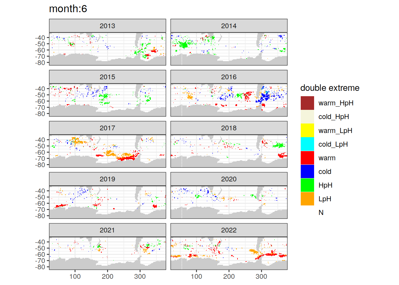
[[7]]
[[8]]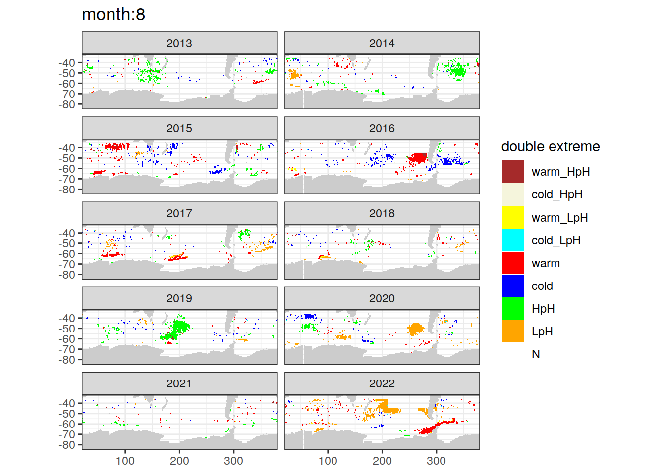
[[9]]
[[10]]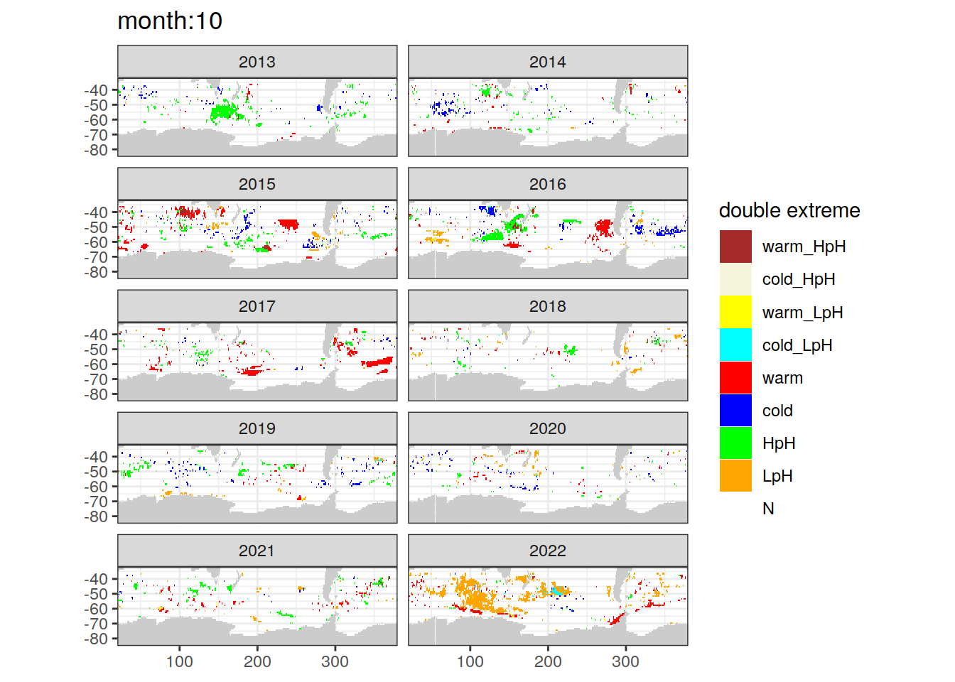
[[11]]
[[12]]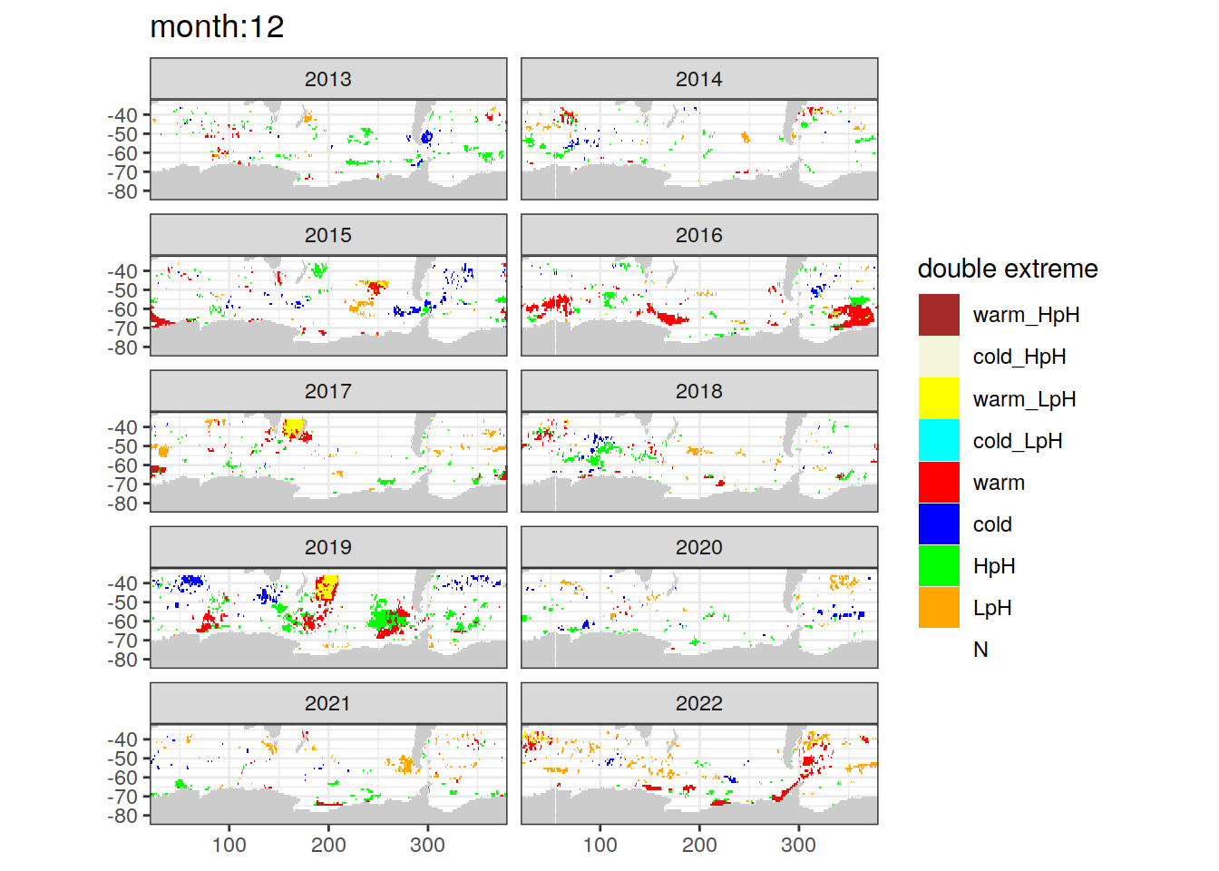
Join Argo profile data
anomaly_field <- anomaly_field %>%
  rename(lat = lat_raw,
         lon = lon_raw) %>%
  filter(year >= 2013)

profile_double_extreme <- inner_join(full_argo, anomaly_field)

# profile_double_extreme <- profile_double_extreme %>%
#   unite('platform_cycle', platform_number:cycle_number, sep = '_', remove = FALSE)
anomaly_field %>%
filter(year >= 2013) %>%
group_split(month) %>%
map(
~map+
geom_tile(data = .x,
aes(x = lon,
y = lat,
fill = double_extreme))+
facet_wrap(~year, ncol = 2)+
scale_fill_manual(values = c('warm_HpH' = 'brown',
'warm_LpH' = 'yellow',
'cold_HpH' = 'beige',
'cold_LpH' = 'cyan',
'cold' = 'blue',
'warm' = 'red',
'LpH' = 'orange',
'HpH' = 'green',
'N' = NA),
na.value = NA)+
geom_point(data = profile_double_extreme,
aes(x = lon,
y = lat),
size = 0.2)+
lims(y = c(-85, -32))+
labs(title = paste0('month:', unique(.x$month)),
fill = 'double extreme')
)[[1]]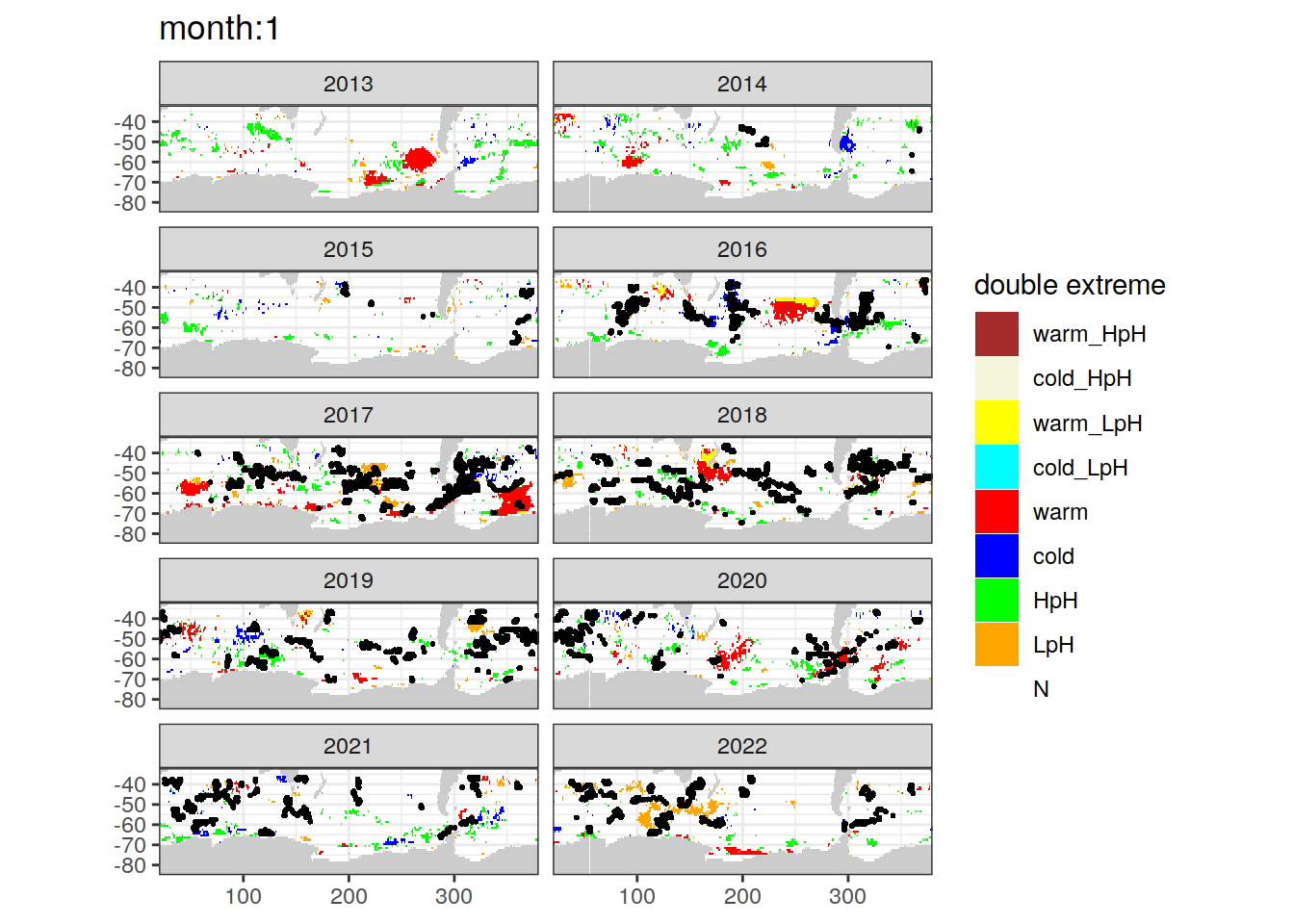
[[2]]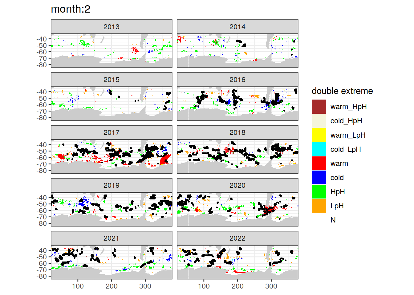
[[3]]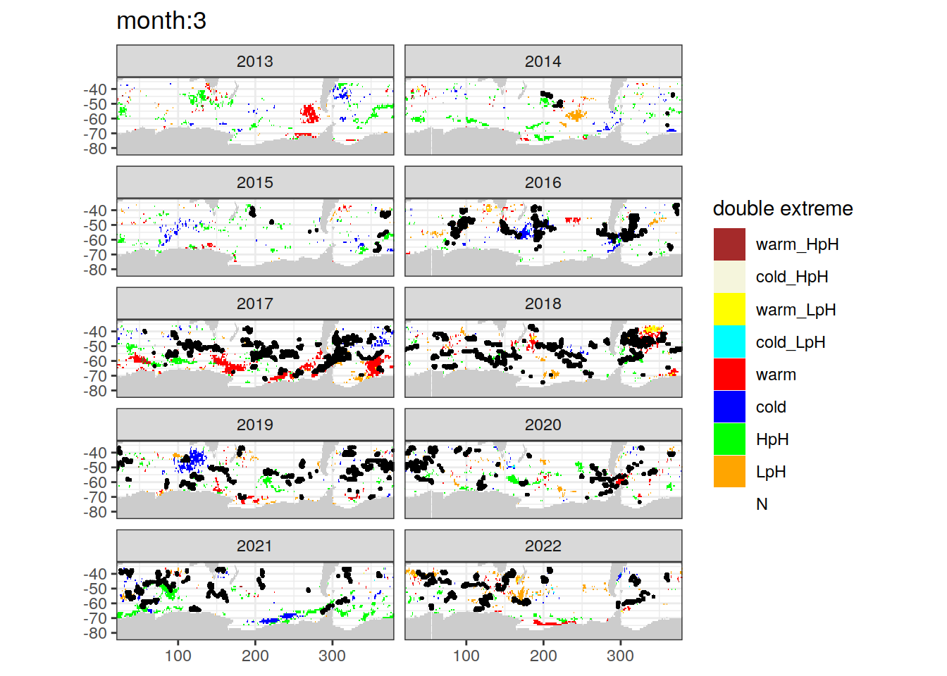
[[4]]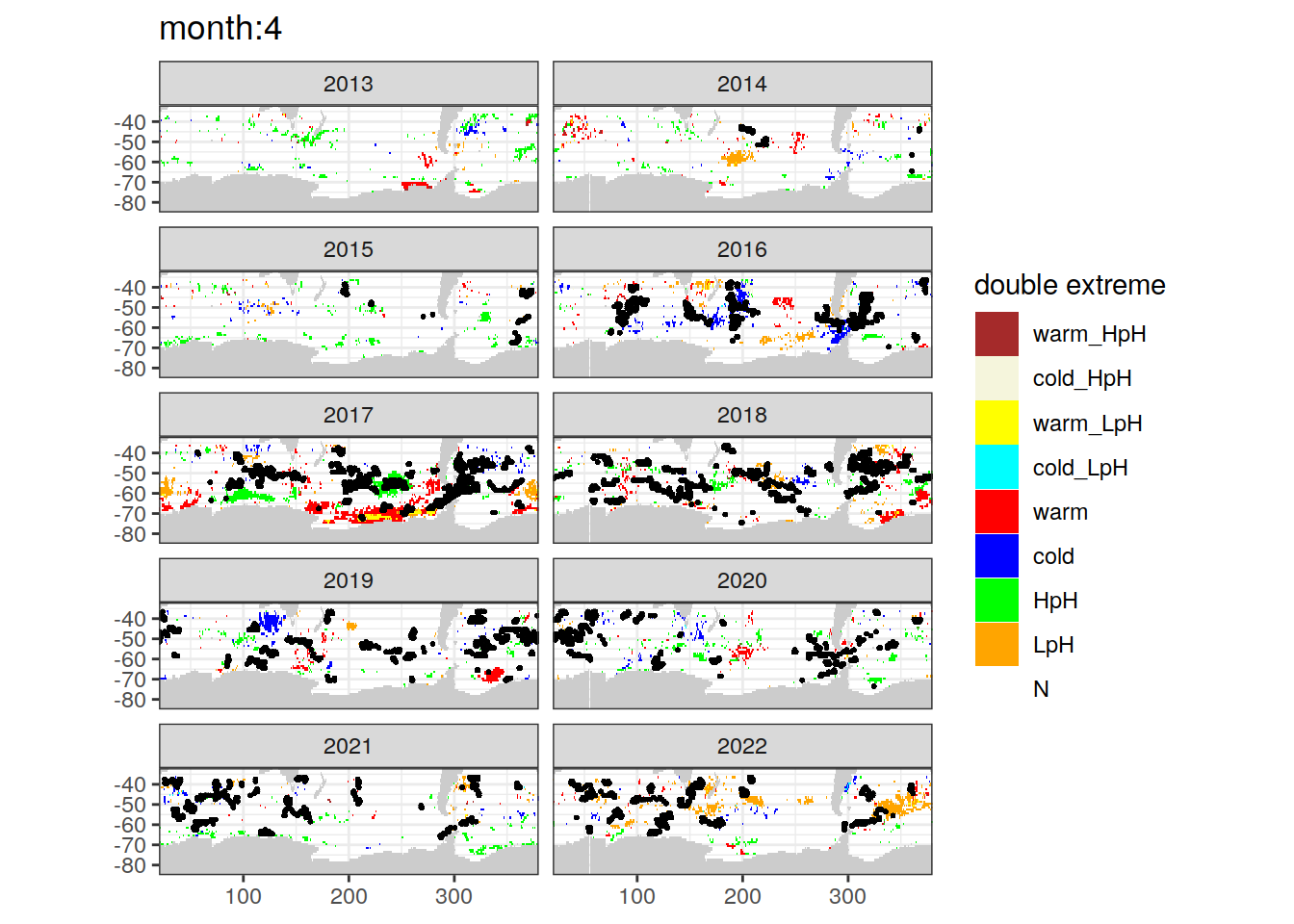
[[5]]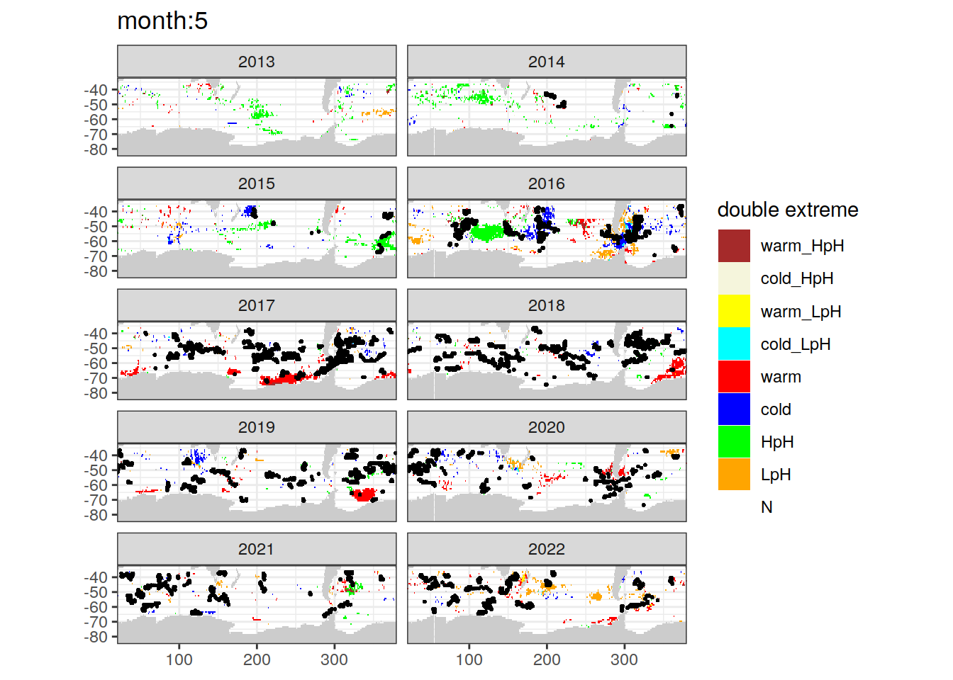
[[6]]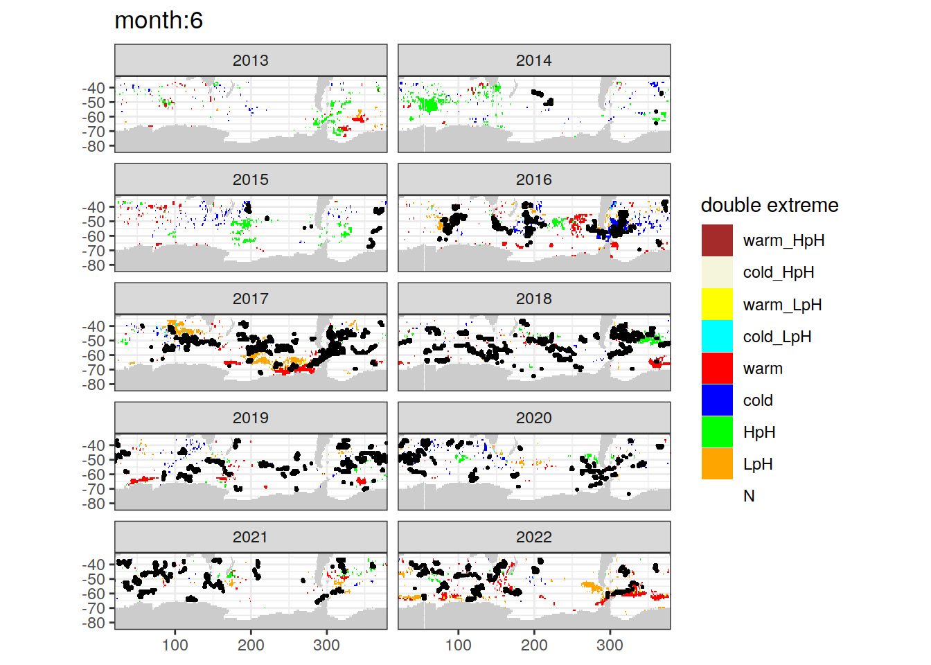
[[7]]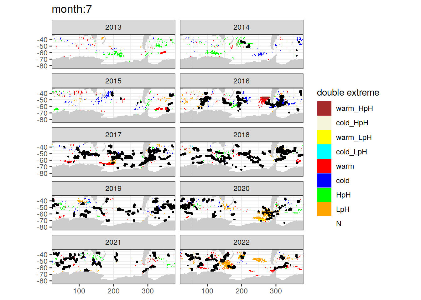
[[8]]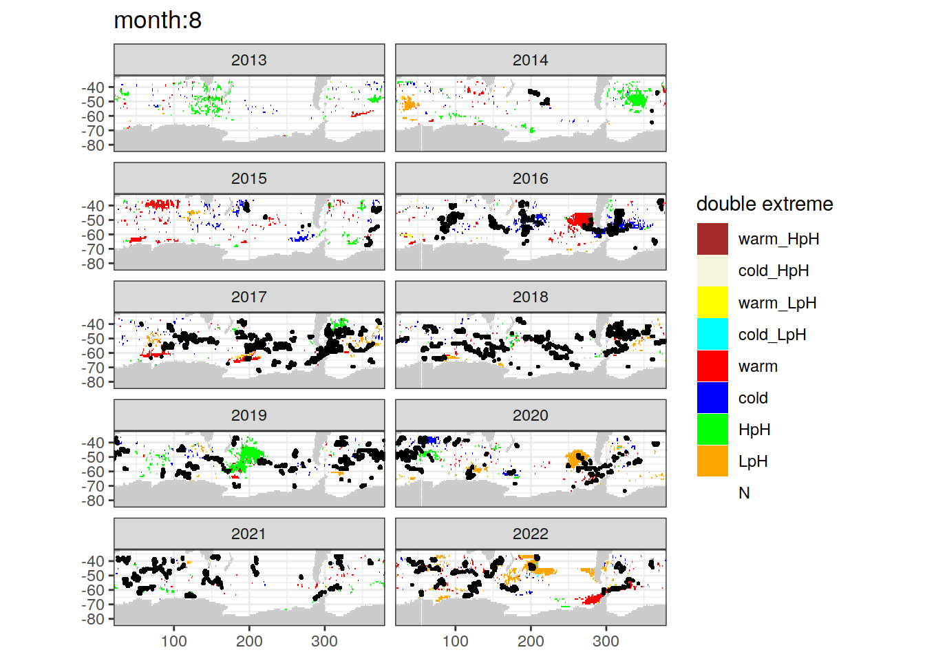
[[9]]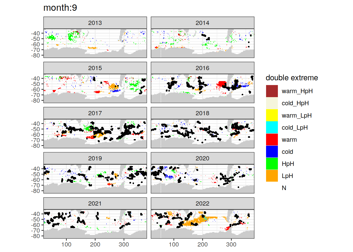
[[10]]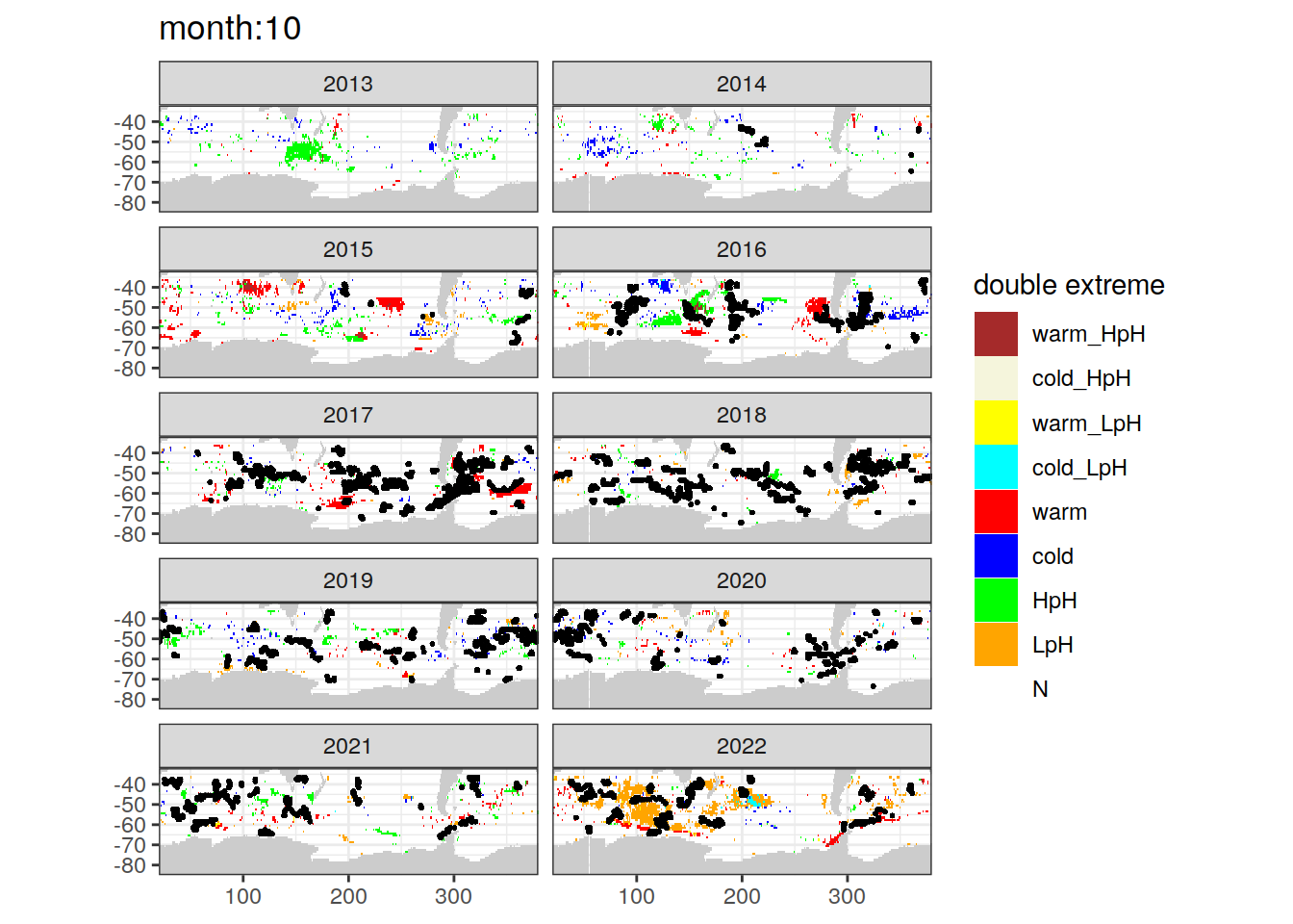
[[11]]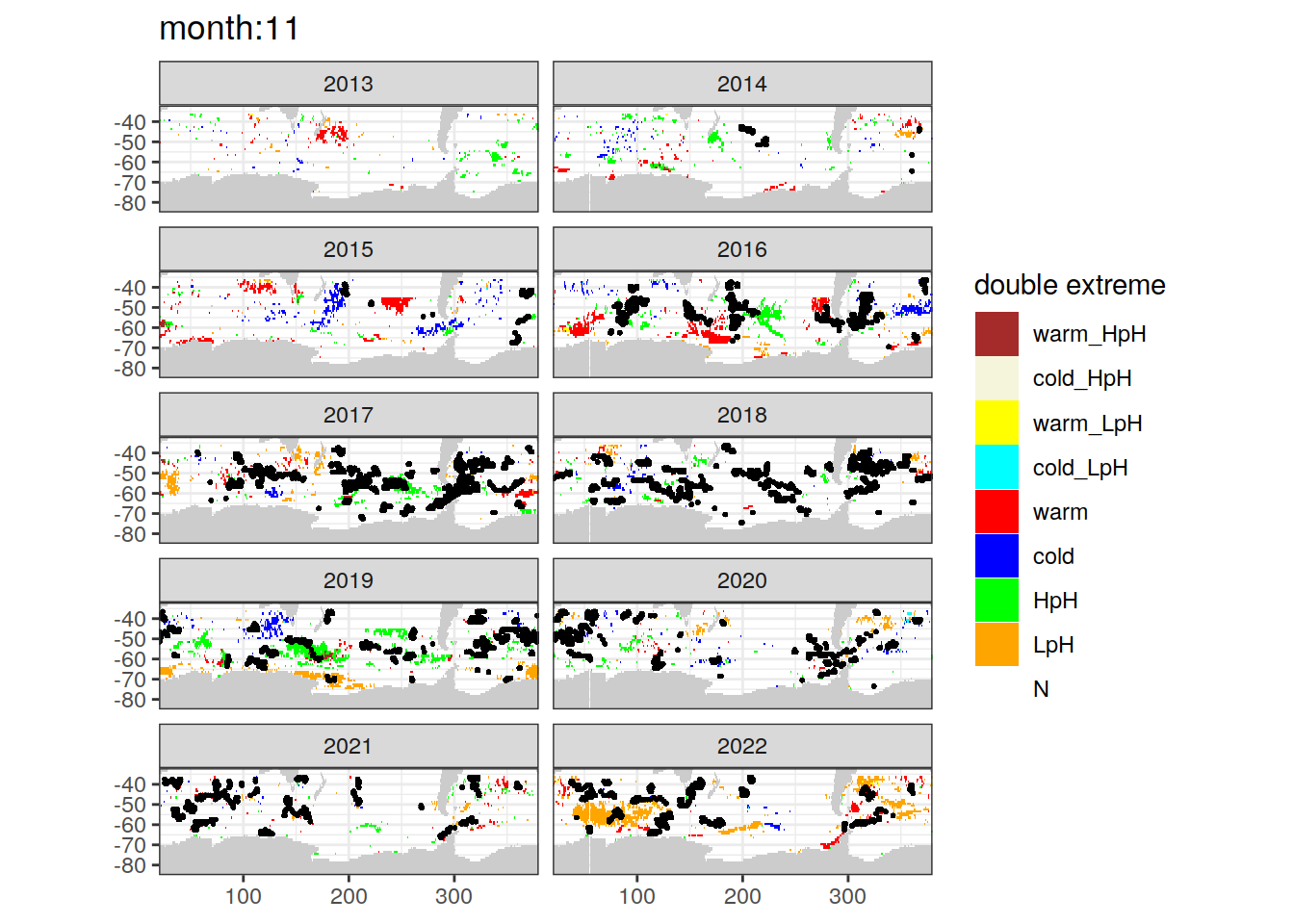
[[12]]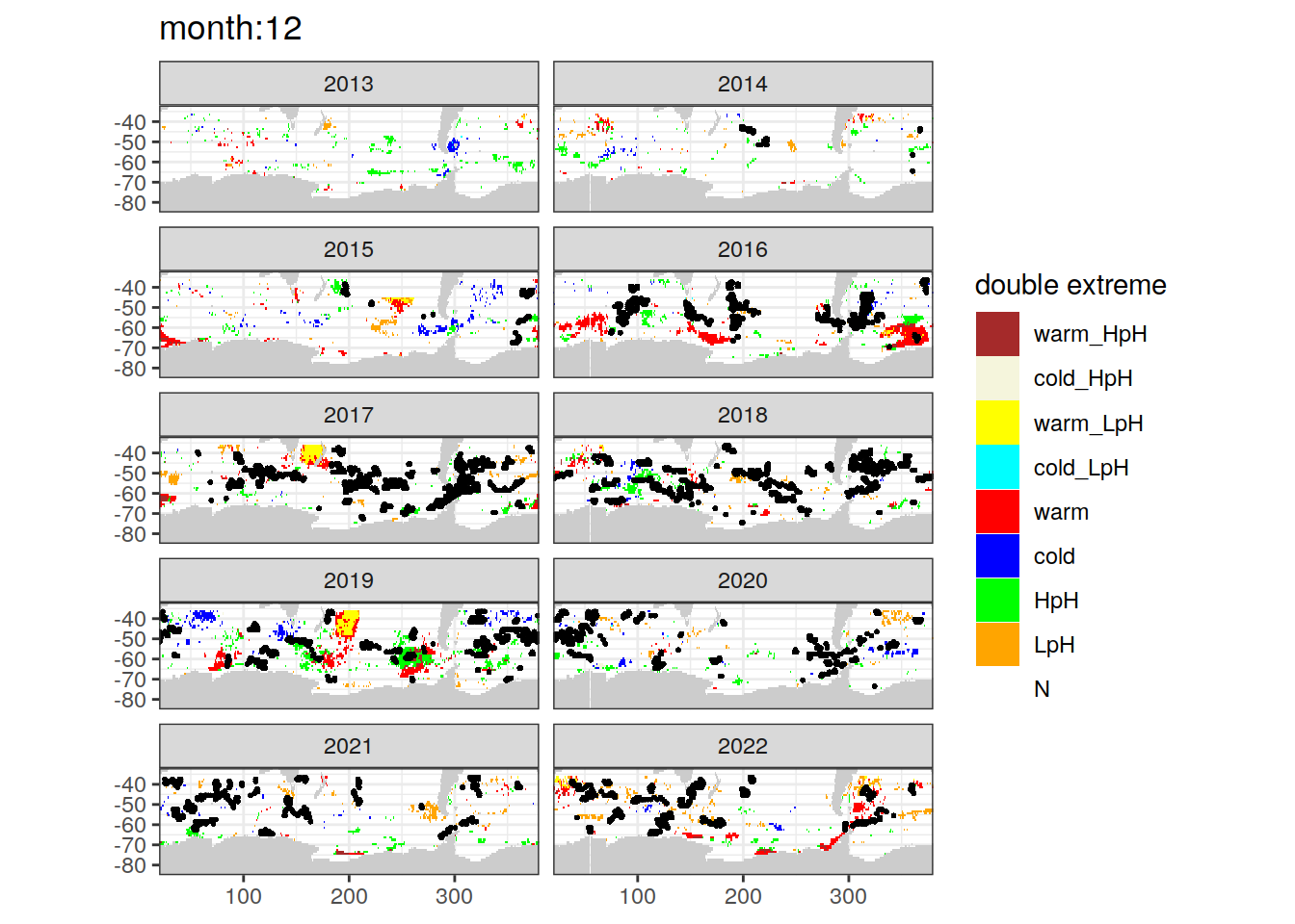
Plot Profiles
Raw
pH
profile_double_extreme %>%
  group_split(biome_name, basin_AIP, year) %>%
  map(
    ~ggplot(data = .x,
            aes(x = pH,
                y = depth,
                group = file_id,
                col = double_extreme))+
      geom_path(data = .x %>% filter(double_extreme == 'N'),
                aes(x = pH,
                    y = depth,
                    group = file_id,
                    col = double_extreme),
                size = 0.3)+
      geom_path(data = .x %>% filter(double_extreme == 'E'),
                aes(x = pH,
                    y = depth,
                    group = file_id,
                    col = double_extreme),
                size = 0.5)+
      scale_y_reverse()+
      scale_color_manual(values = c('N' = 'gray', 'E' = 'red'))+
      facet_wrap(~month, ncol = 6)+
      labs(title = paste0('biome: ', unique(.x$biome_name), '| ', unique(.x$basin_AIP), '| ', unique(.x$year)),
           col = 'double extreme',
           x = 'Argo pH',
           y = 'depth')
  )
[[1]]
[[2]]
[[3]]
[[4]]
[[5]]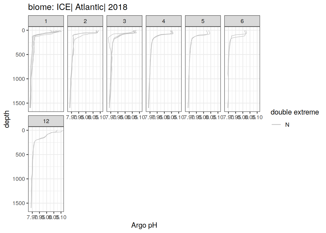
[[6]]
[[7]]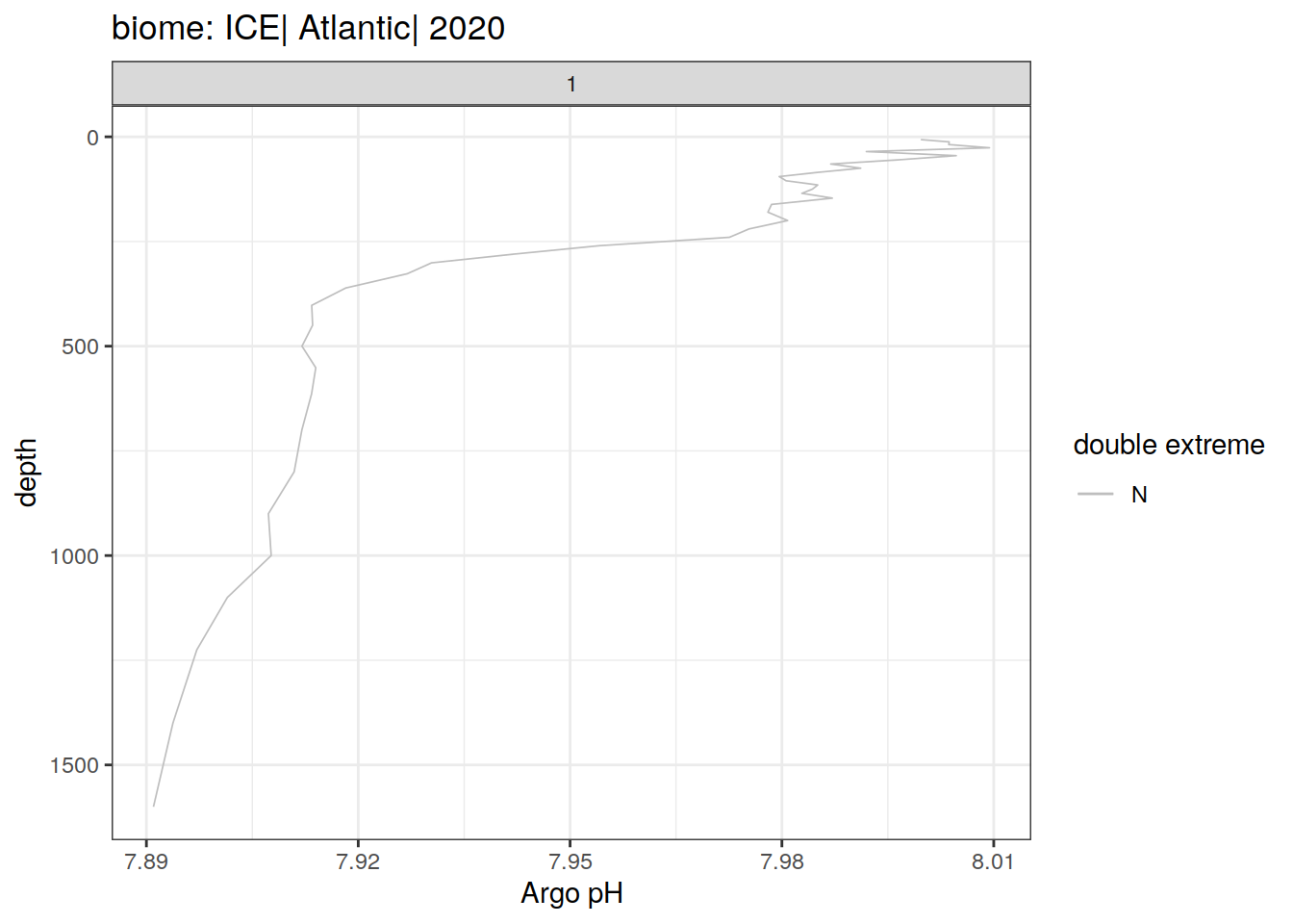
[[8]]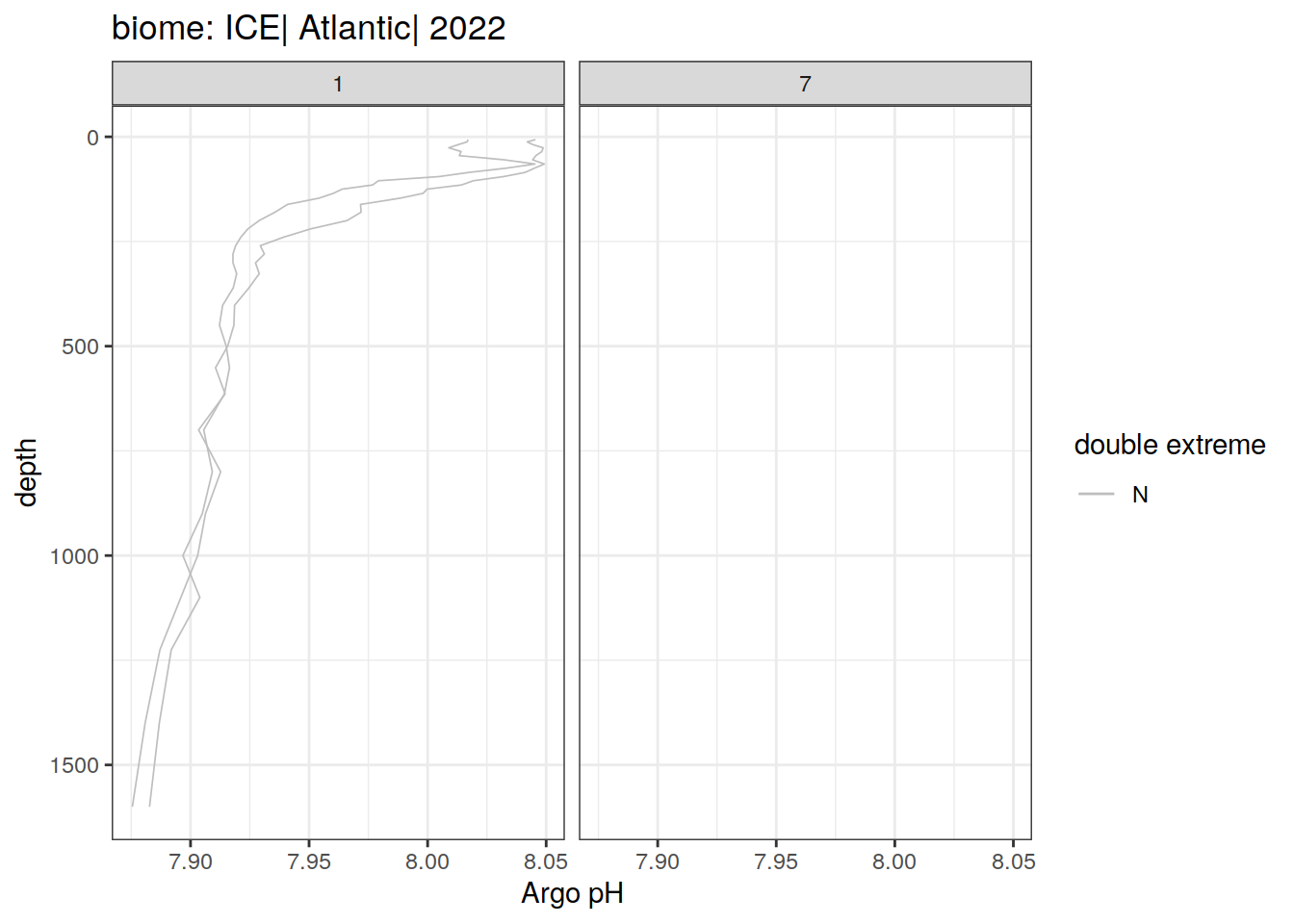
[[9]]
[[10]]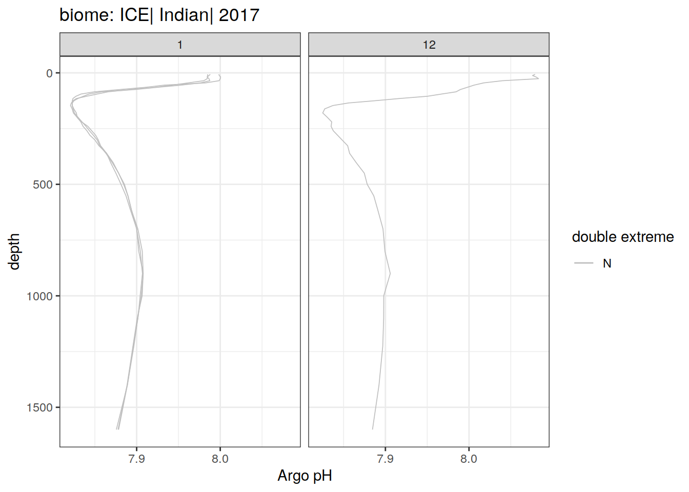
[[11]]
[[12]]
[[13]]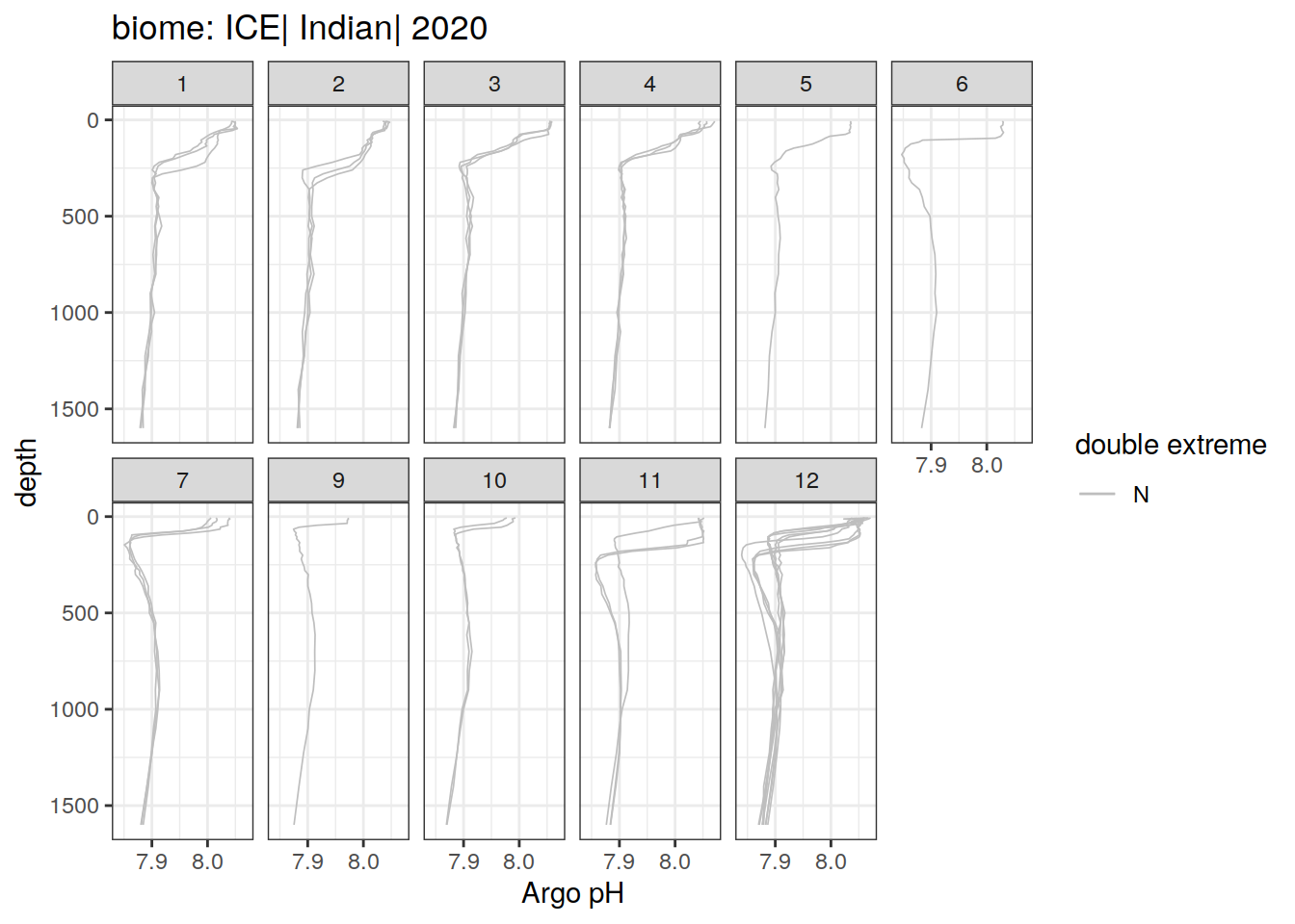
[[14]]
[[15]]
[[16]]
[[17]]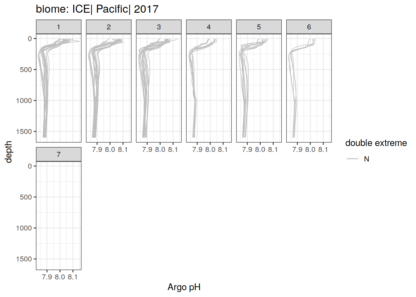
[[18]]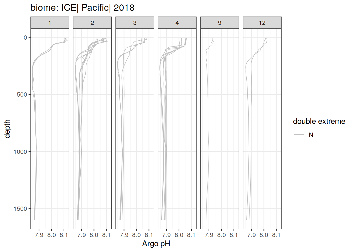
[[19]]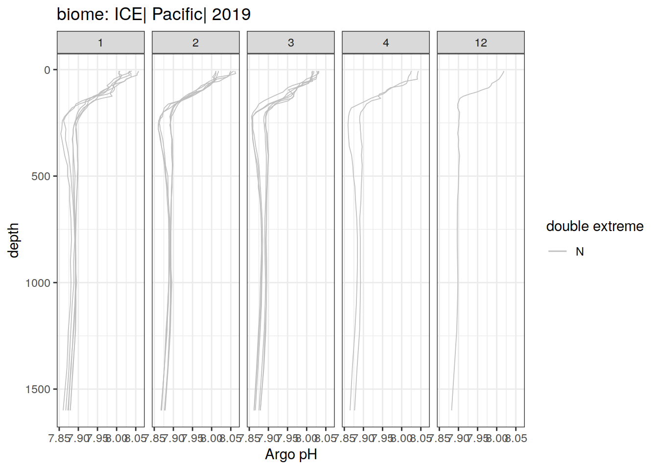
[[20]]
[[21]]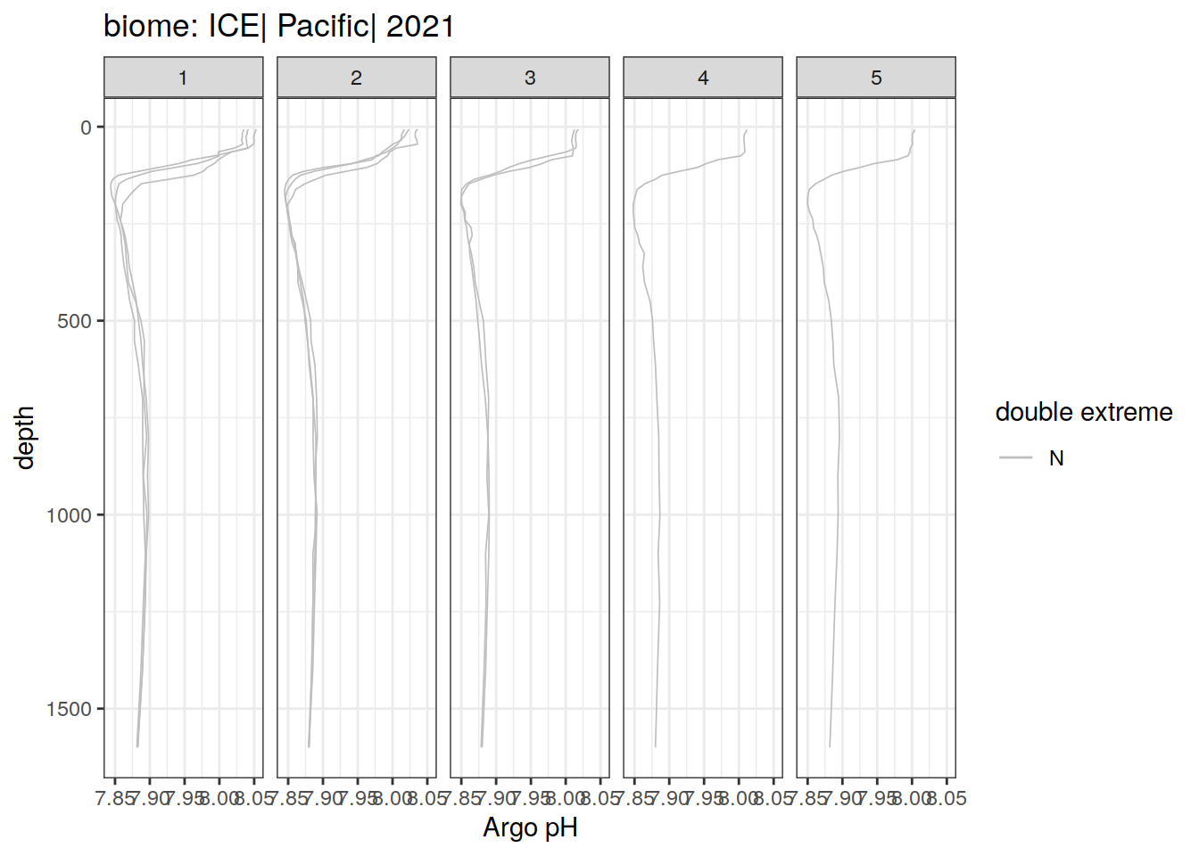
[[22]]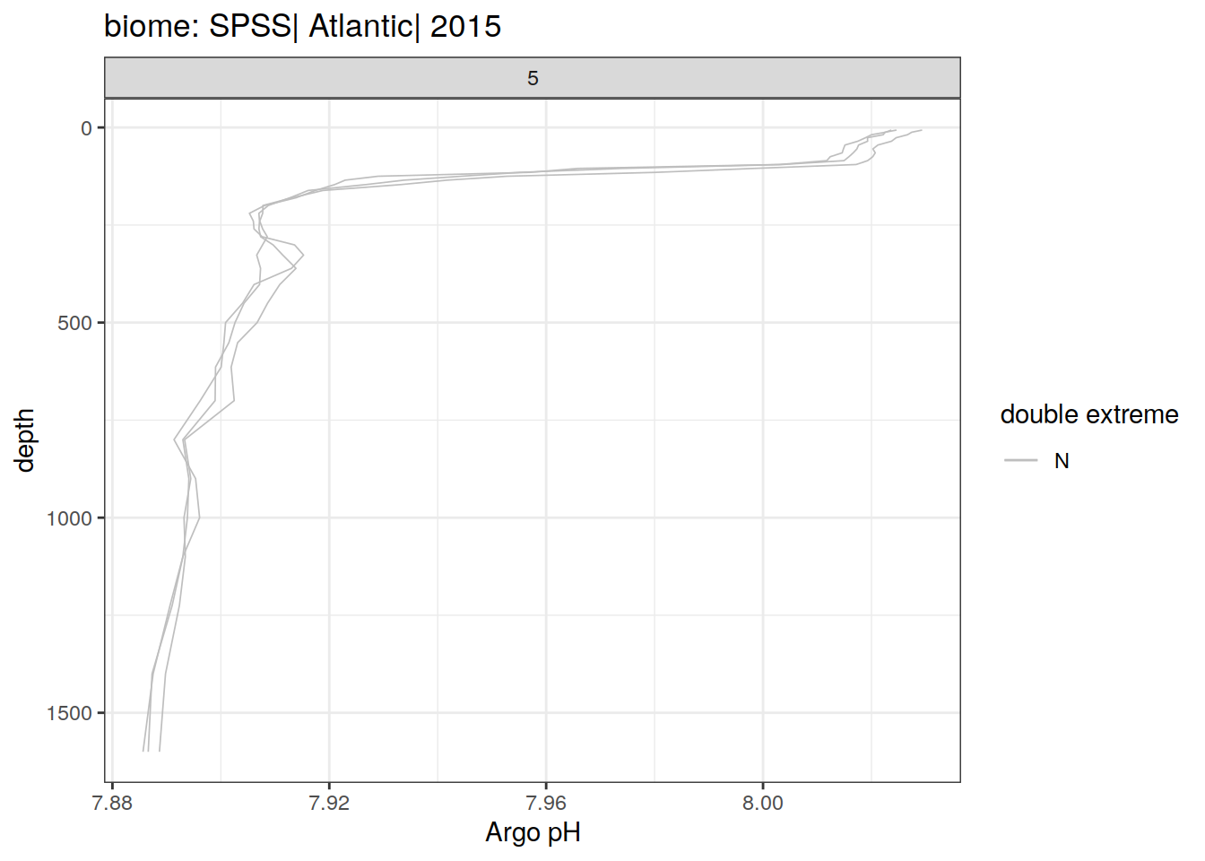
[[23]]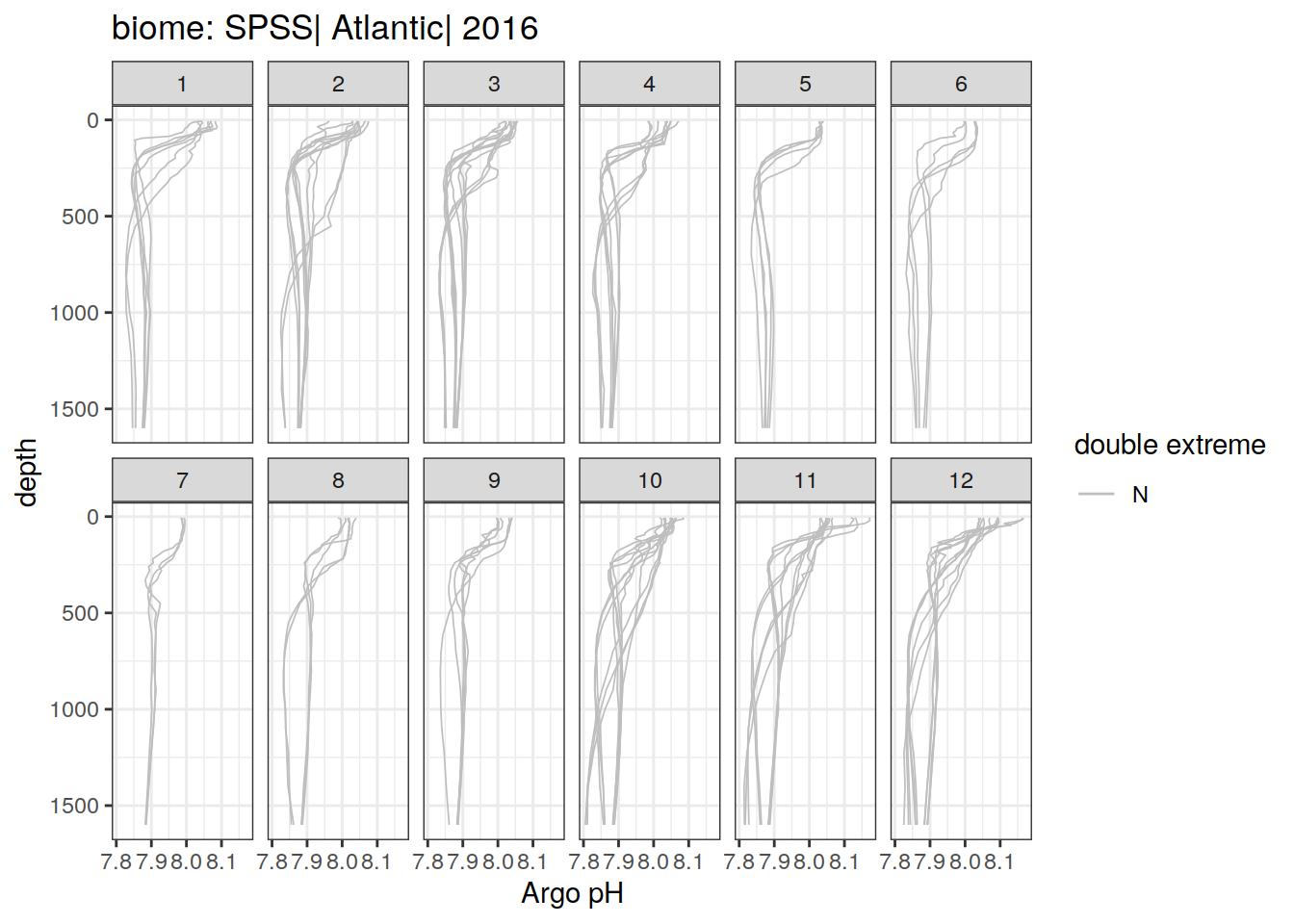
[[24]]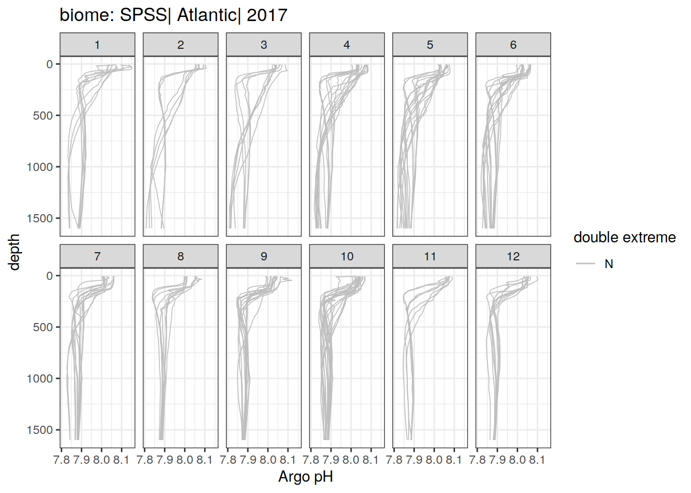
[[25]]
[[26]]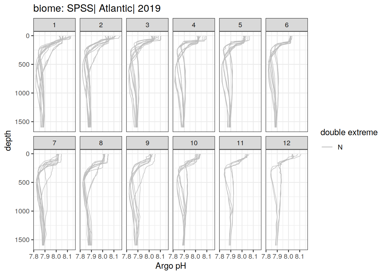
[[27]]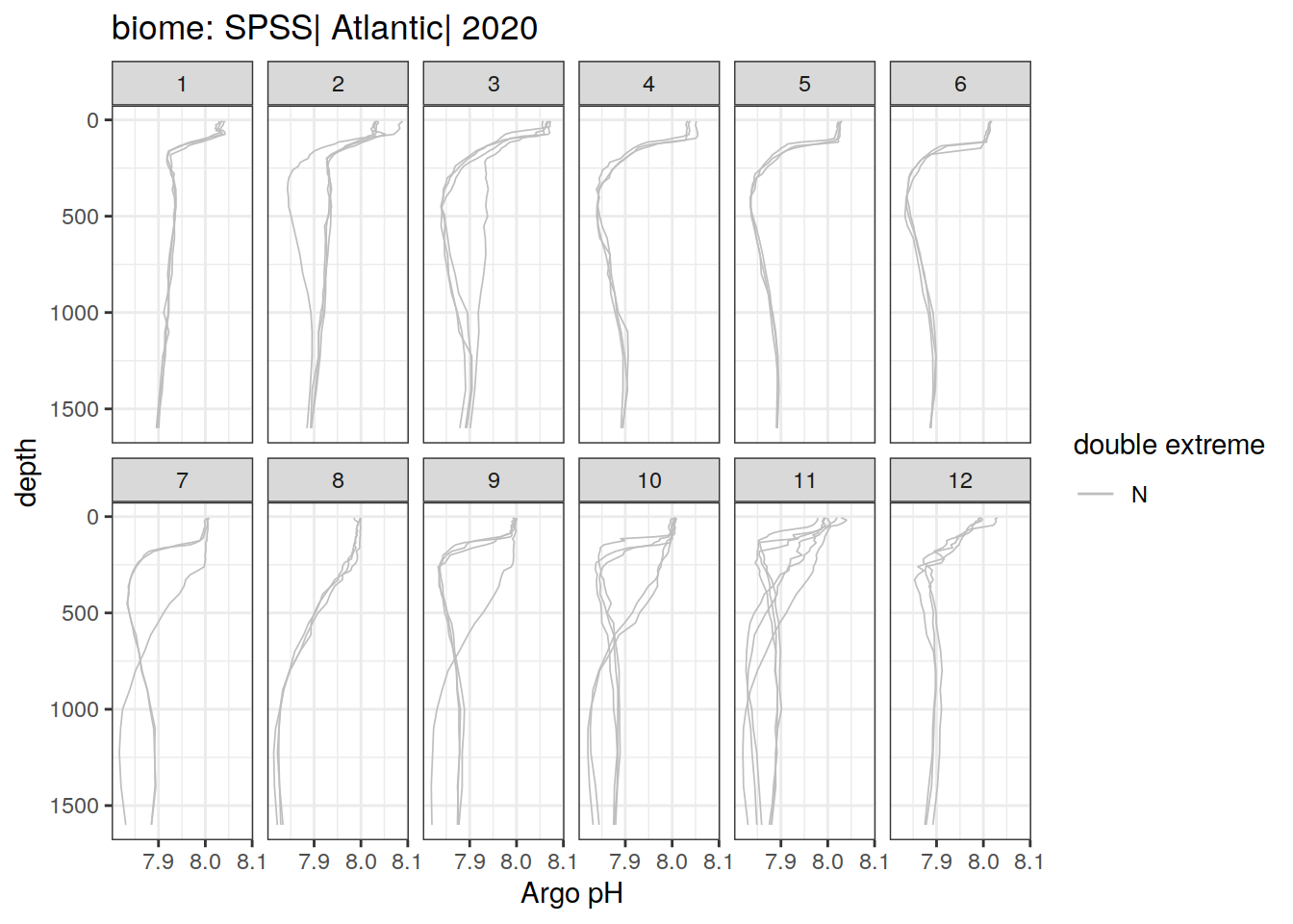
[[28]]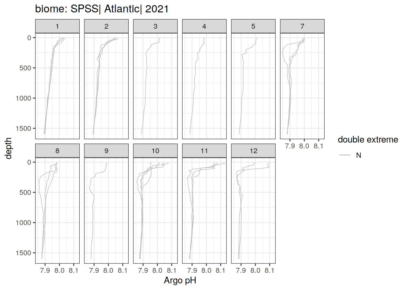
[[29]]
[[30]]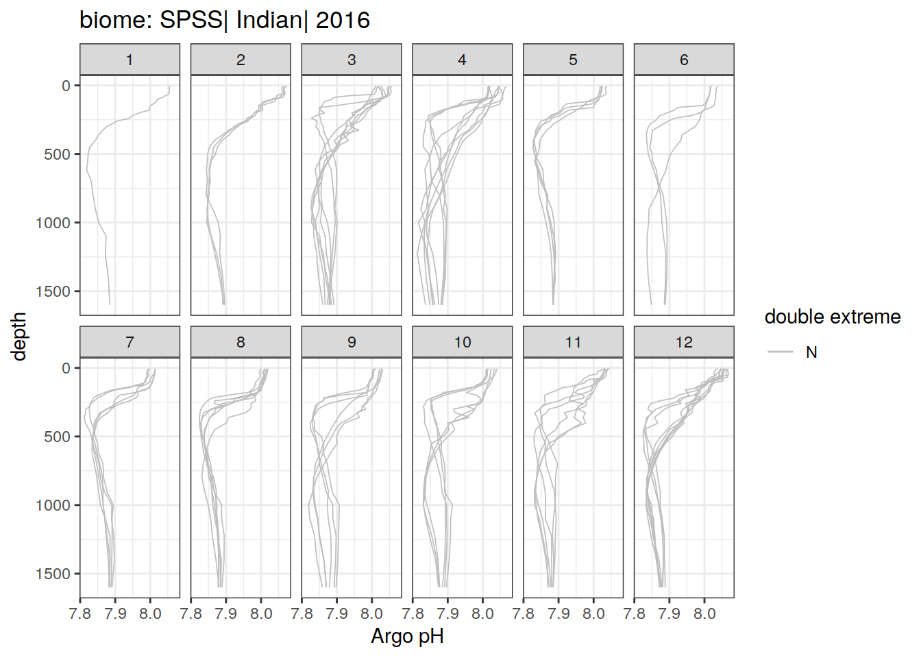
[[31]]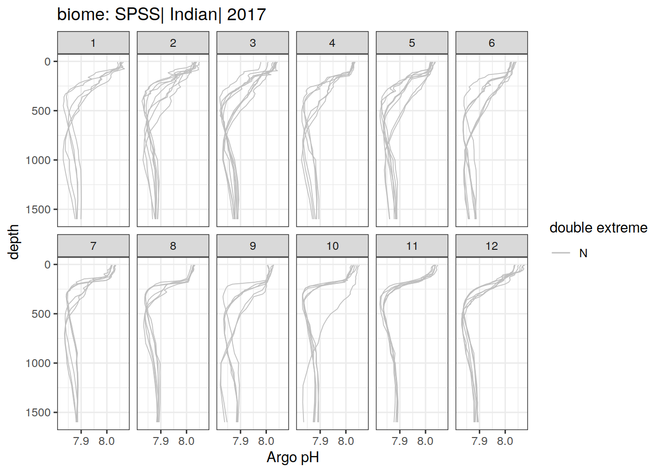
[[32]]
[[33]]
[[34]]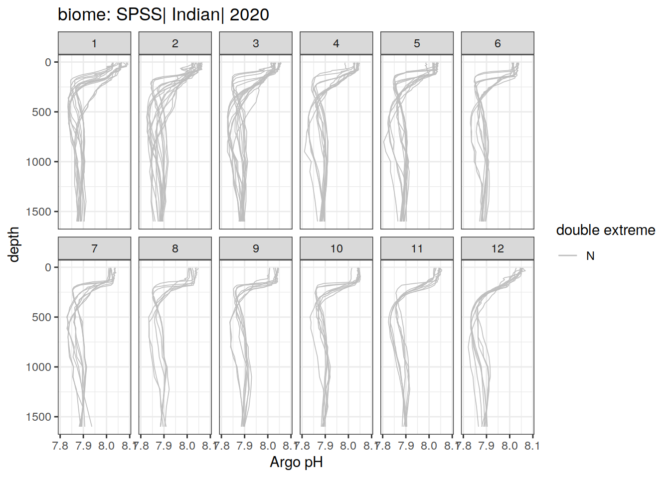
[[35]]
[[36]]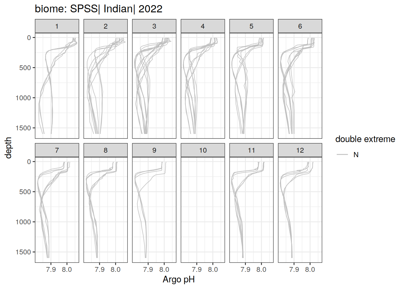
[[37]]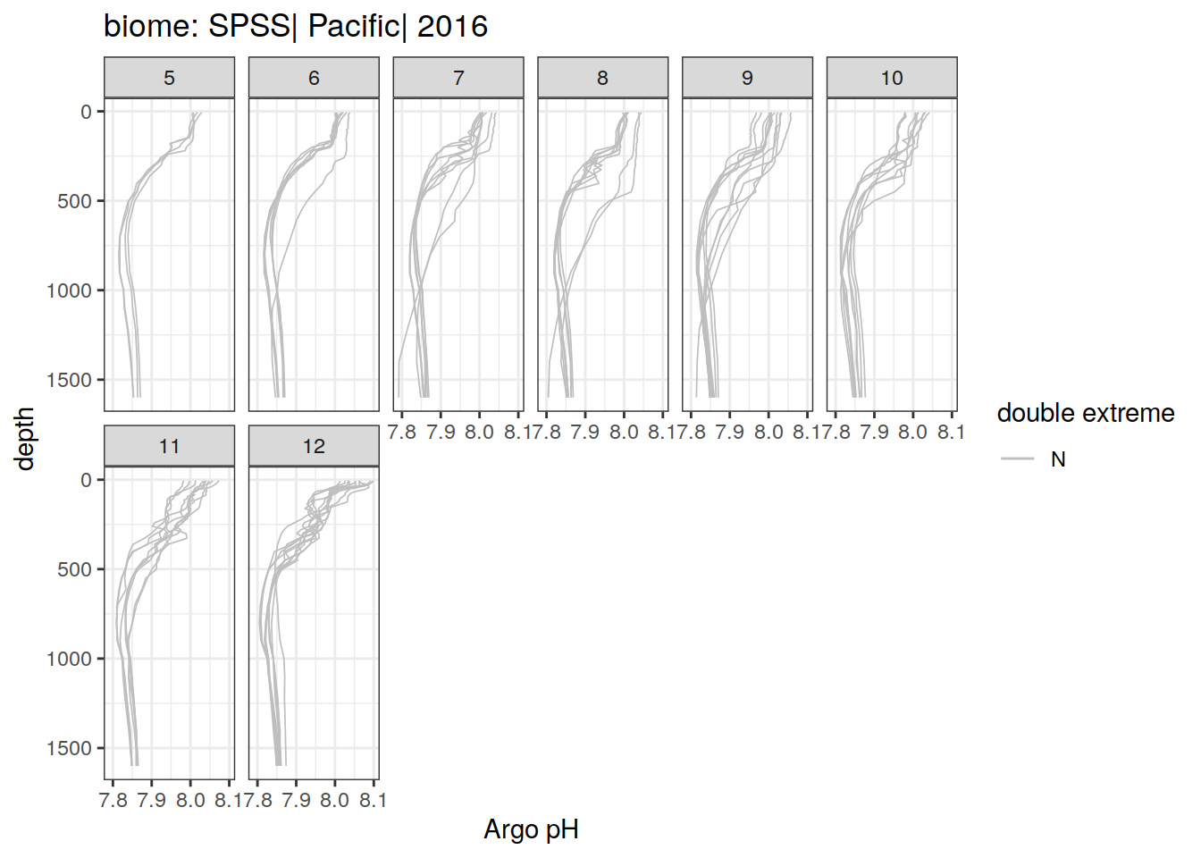
[[38]]
[[39]]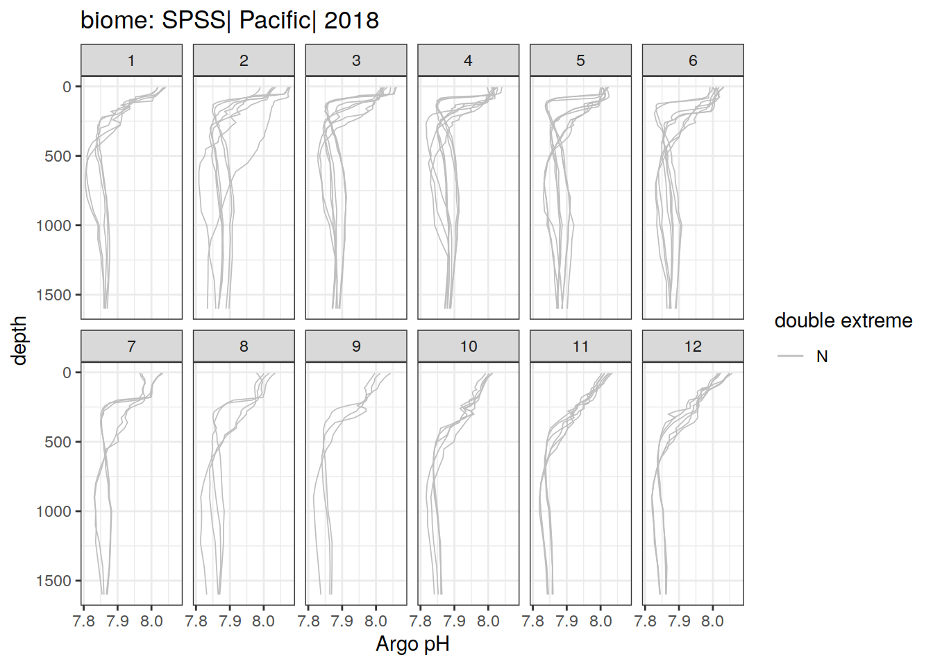
[[40]]
[[41]]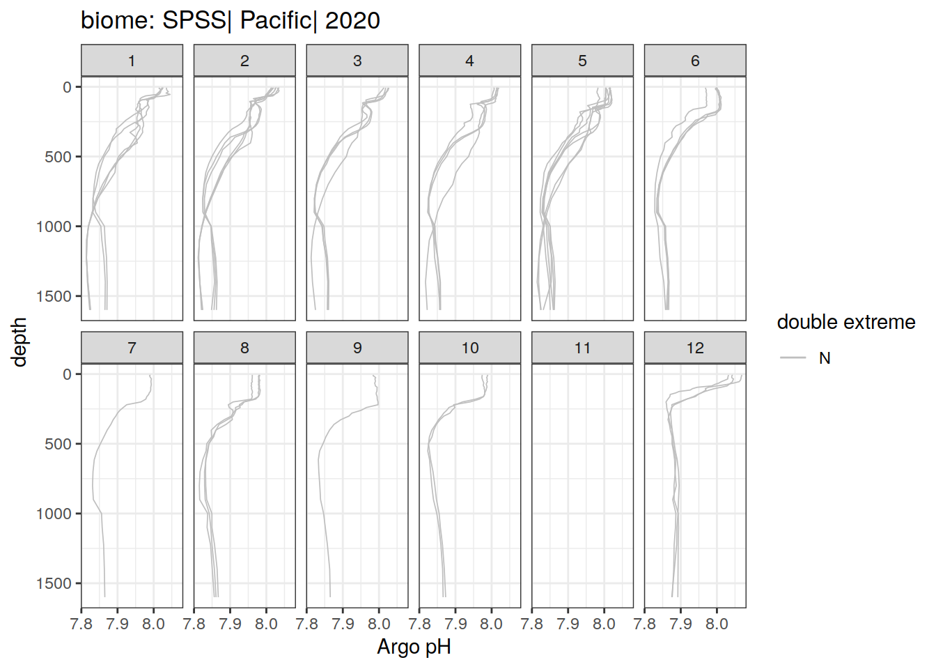
[[42]]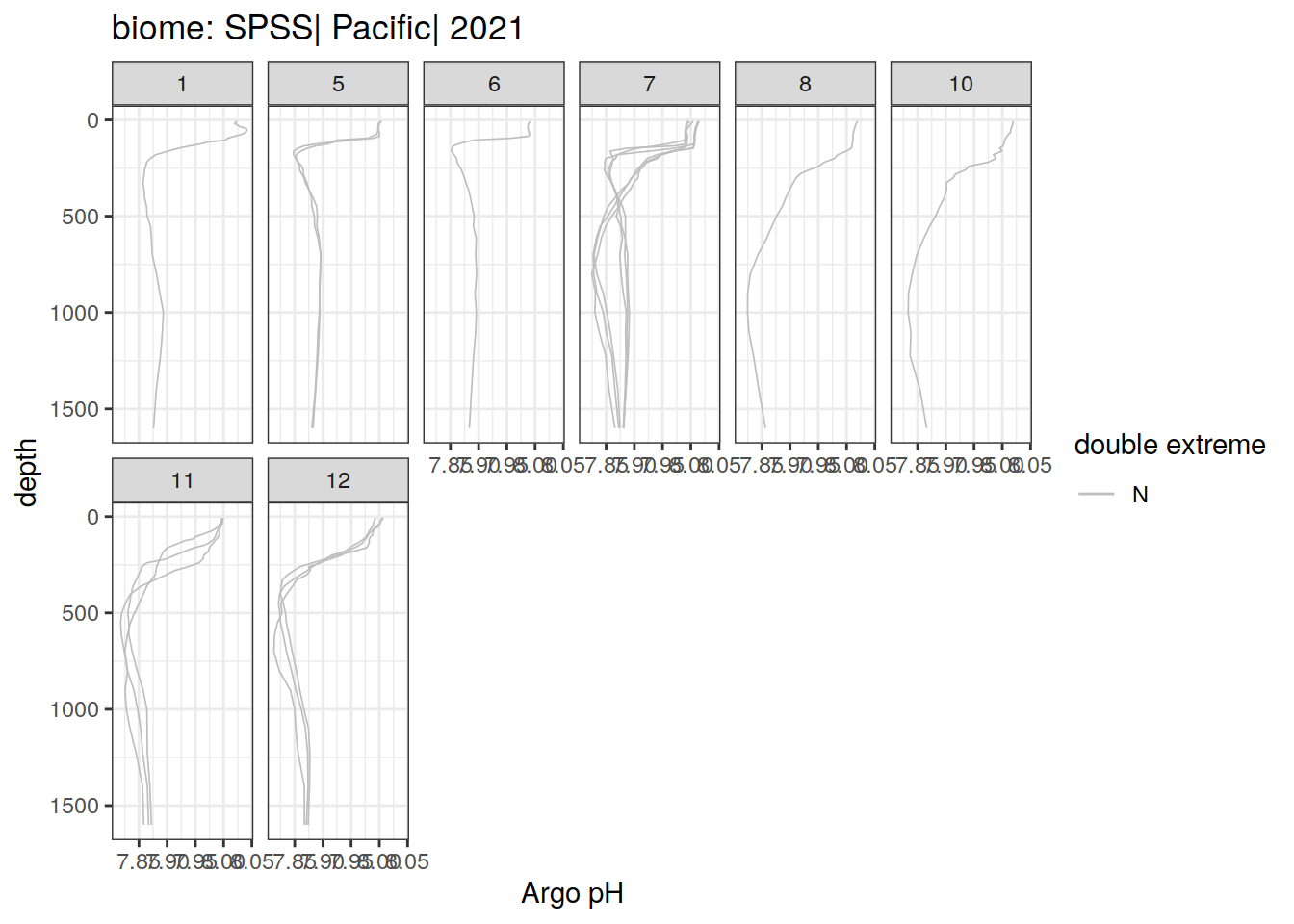
[[43]]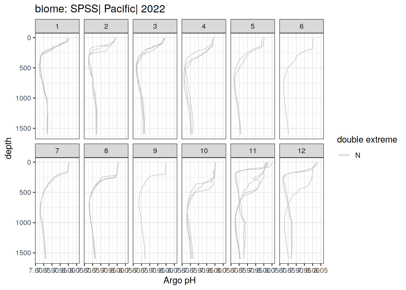
[[44]]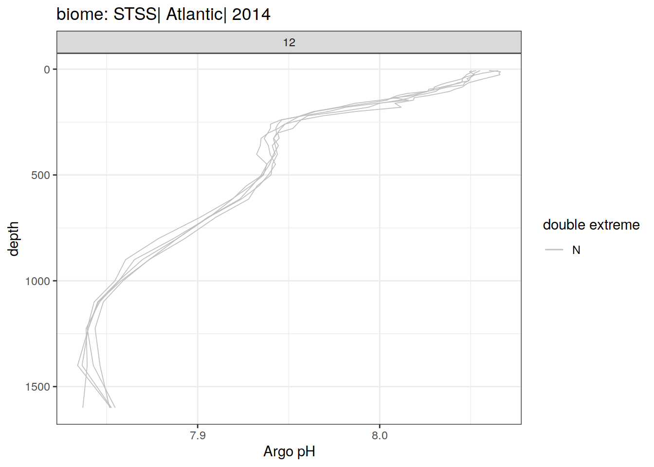
[[45]]
[[46]]
[[47]]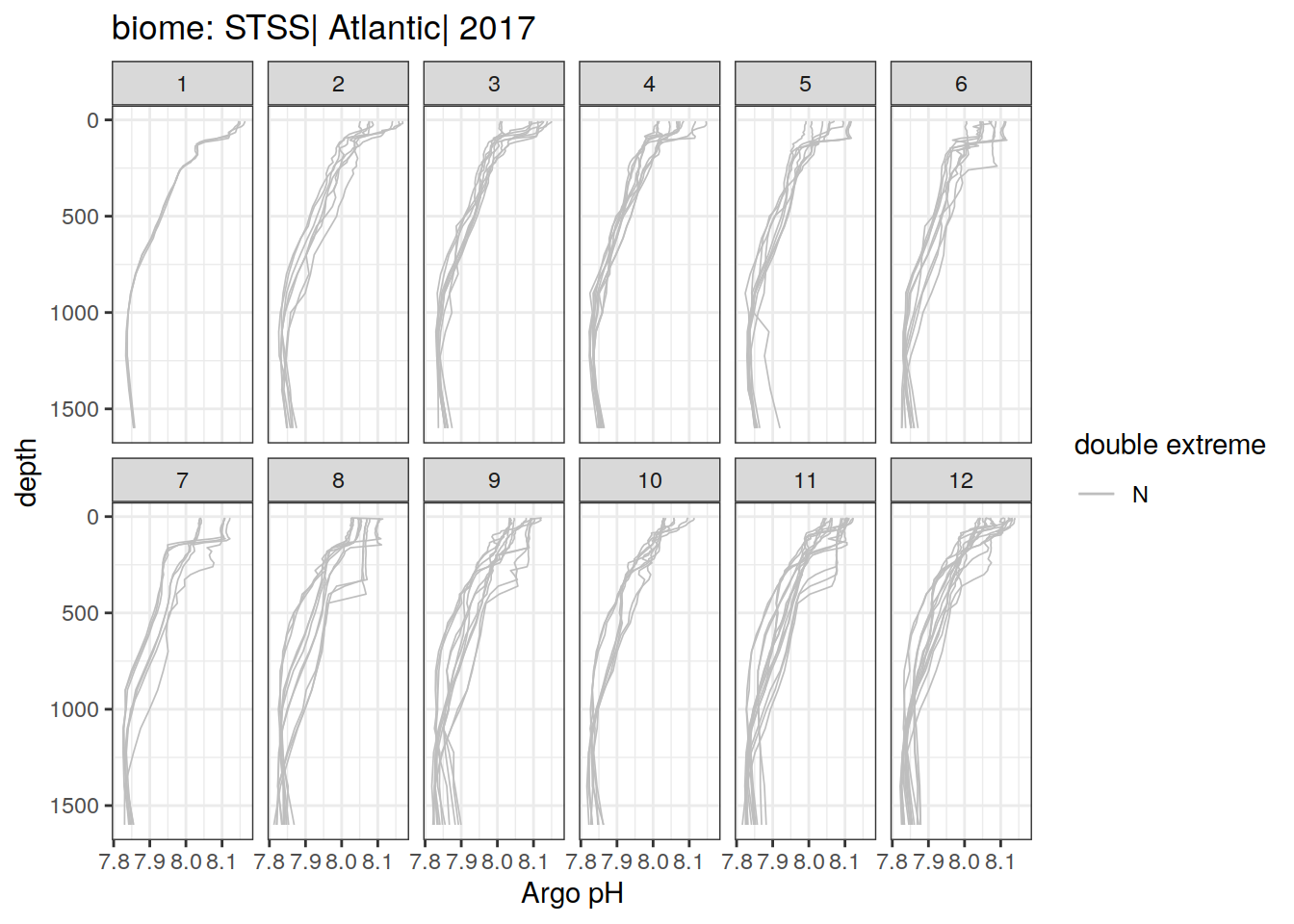
[[48]]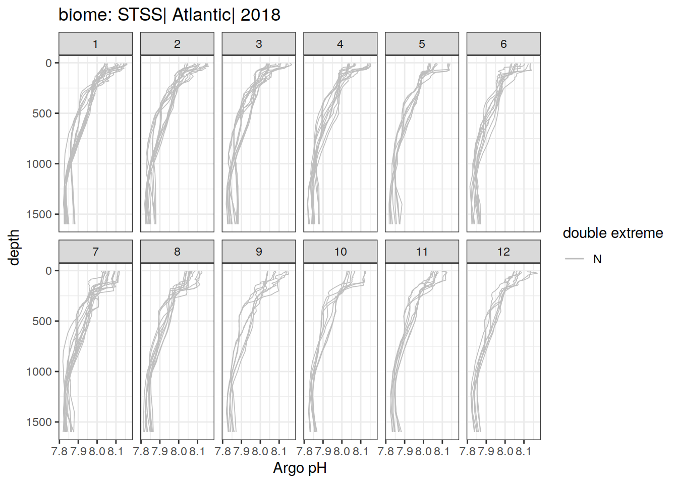
[[49]]
[[50]]
[[51]]
[[52]]
[[53]]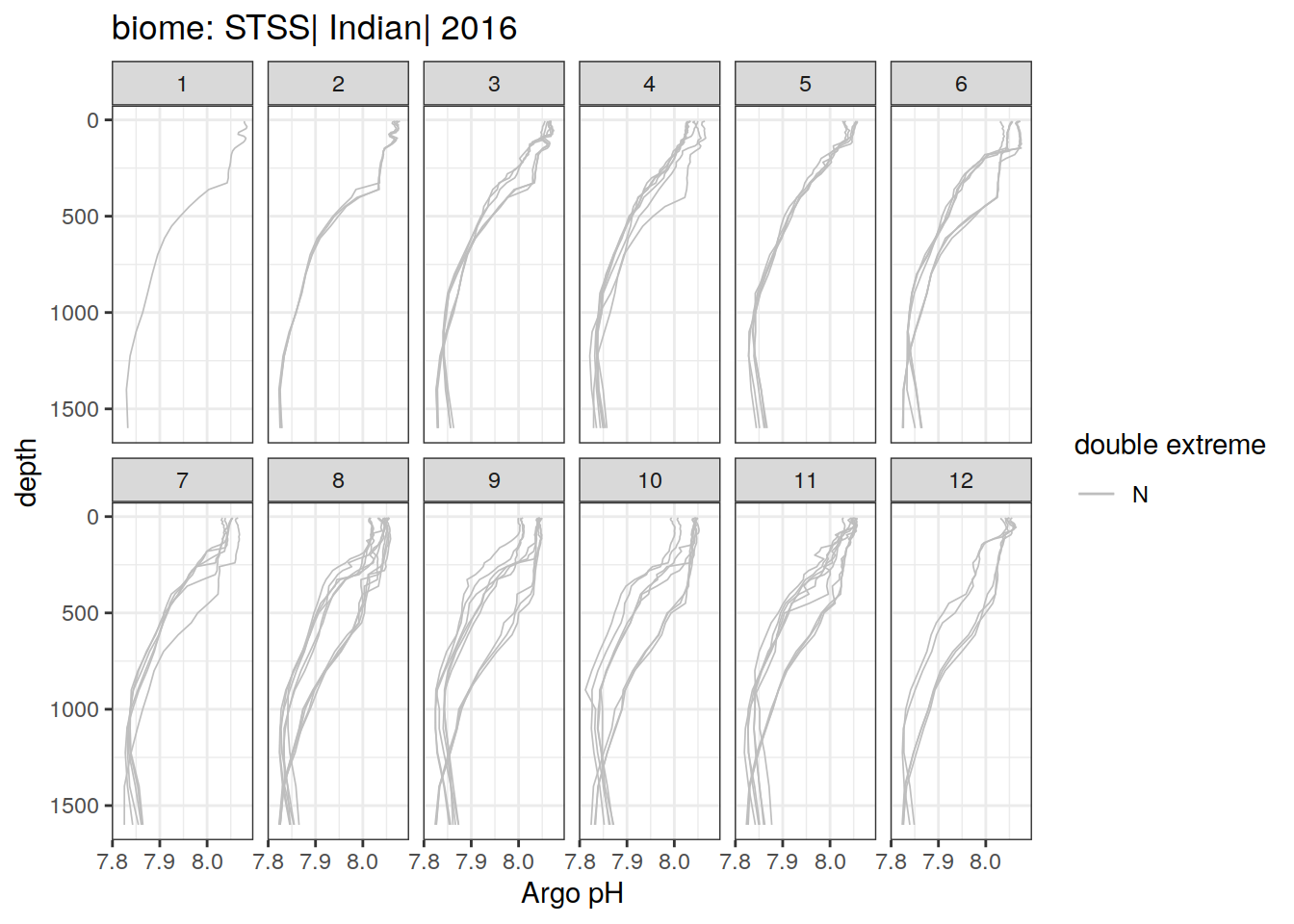
[[54]]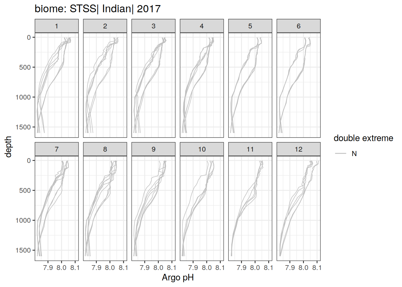
[[55]]
[[56]]
[[57]]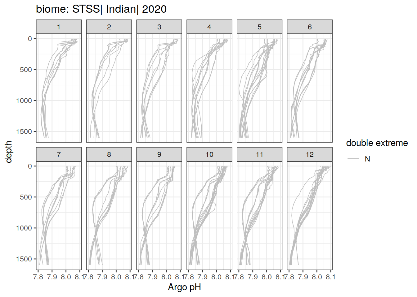
[[58]]
[[59]]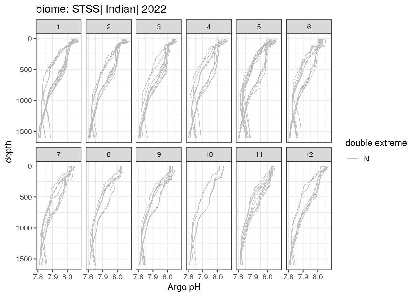
[[60]]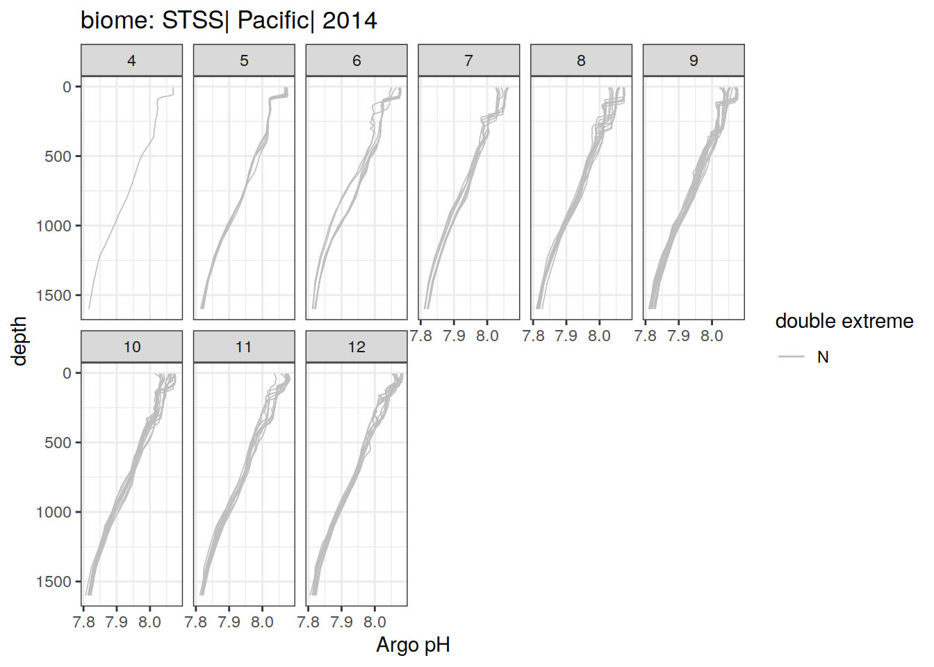
[[61]]
[[62]]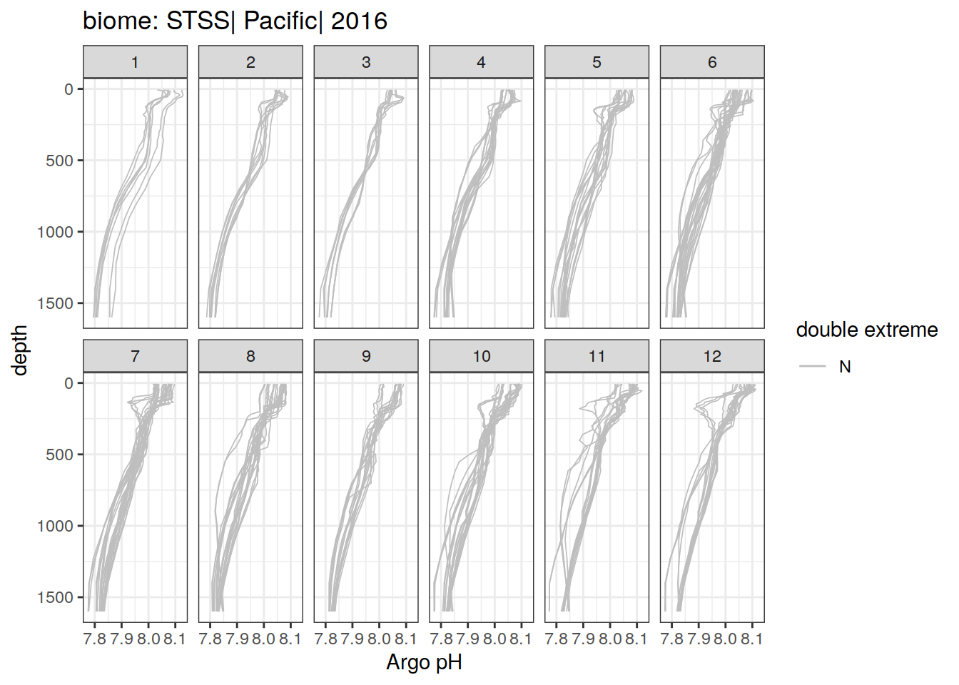
[[63]]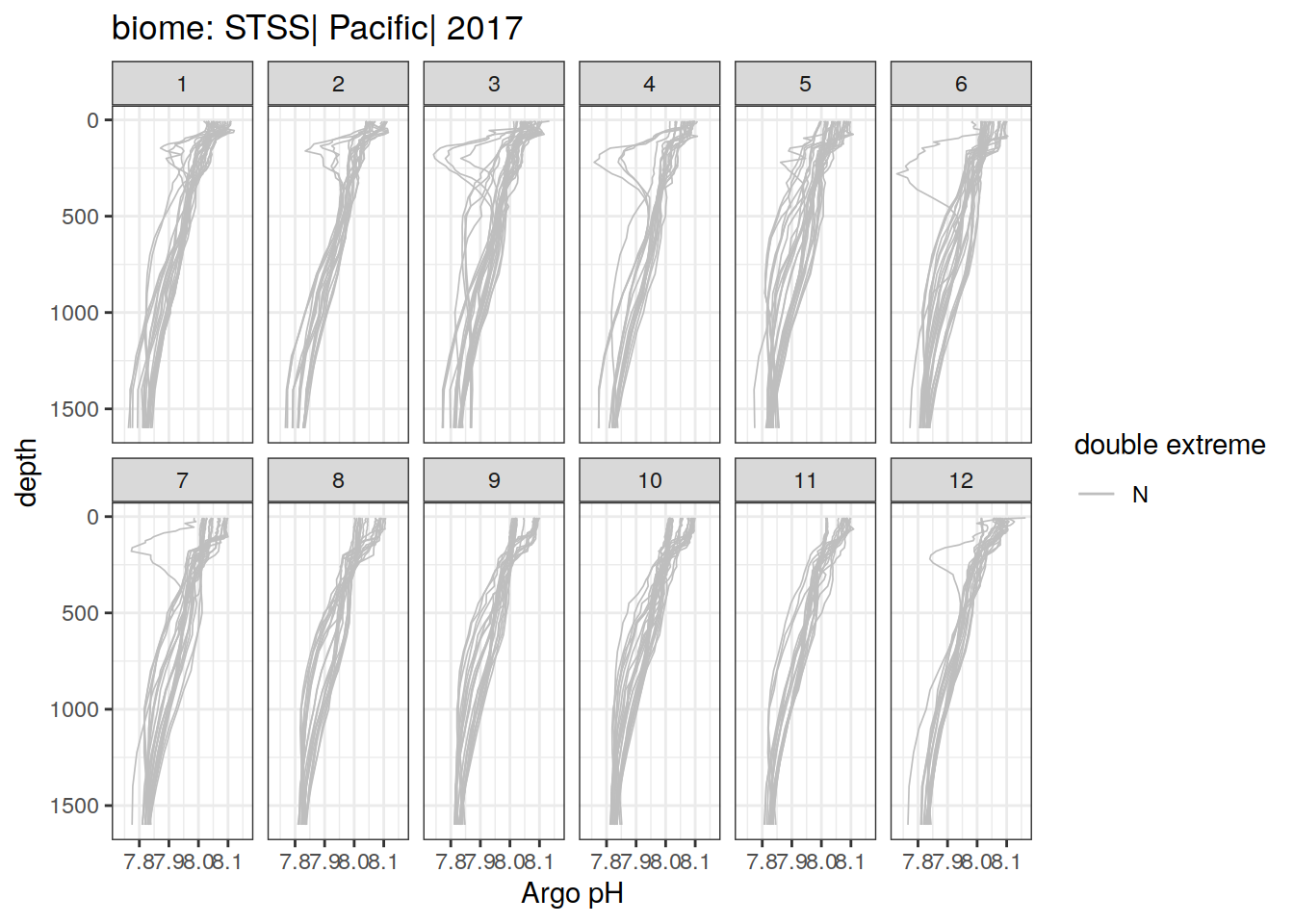
[[64]]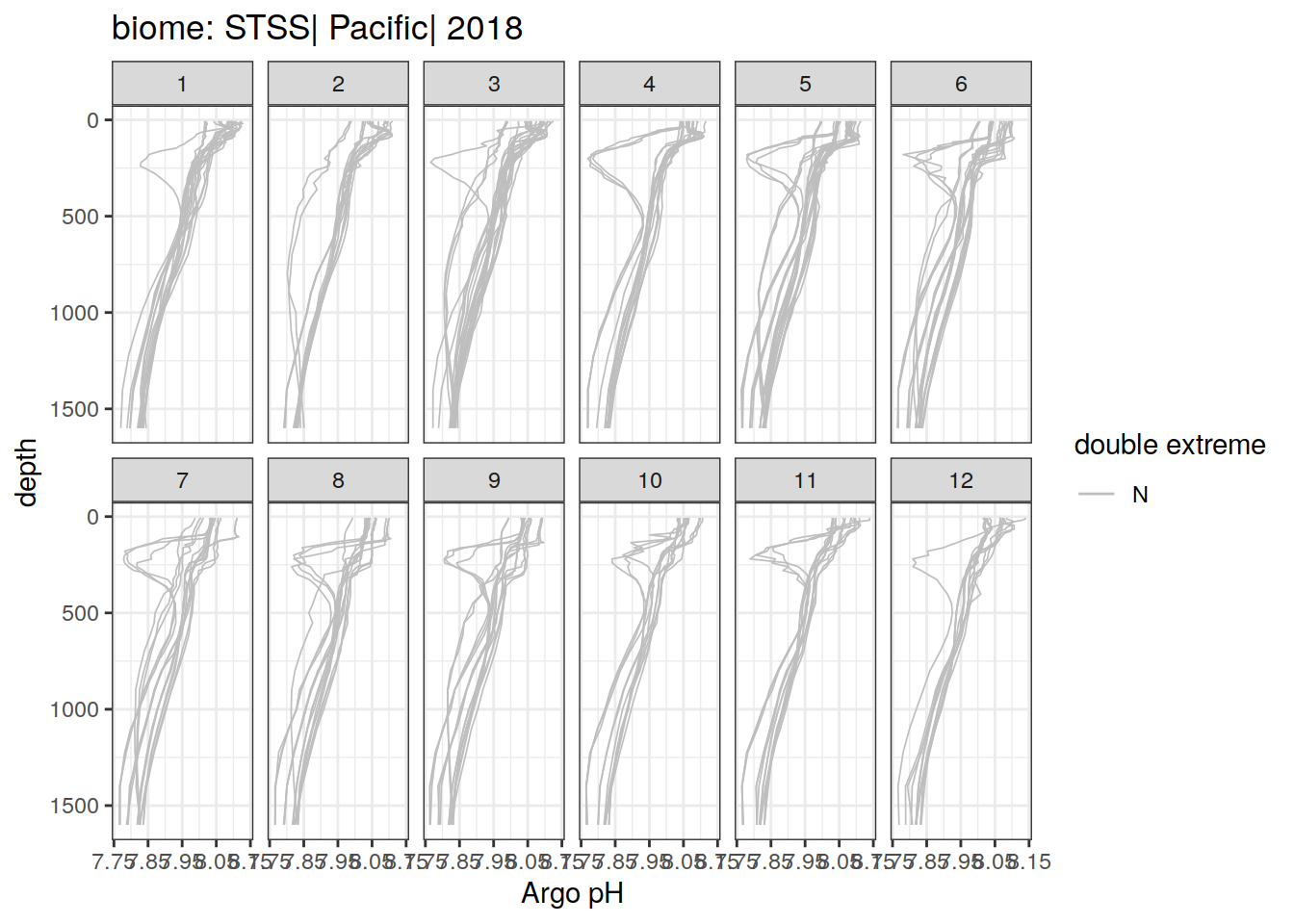
[[65]]
[[66]]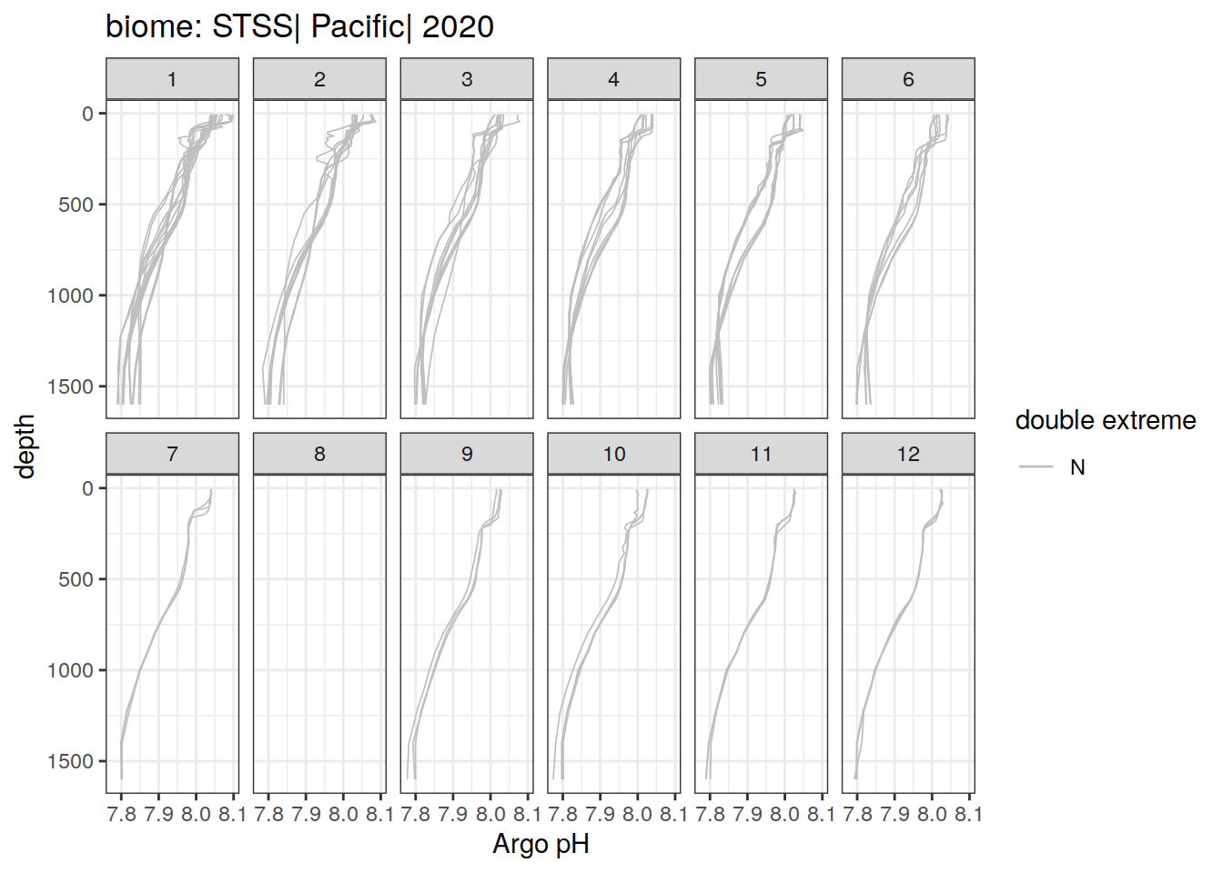
[[67]]
[[68]]
Temperature
profile_double_extreme %>%
  group_split(biome_name, basin_AIP, year) %>%
  map(
    ~ggplot(data = .x,
            aes(x = temp,
                y = depth,
                group = file_id,
                col = double_extreme))+
      geom_path(data = .x %>% filter(double_extreme == 'N'),
                aes(x = temp,
                    y = depth,
                    group = file_id,
                    col = double_extreme),
                size = 0.3)+
      geom_path(data = .x %>% filter(double_extreme == 'E'),
                aes(x = temp,
                    y = depth,
                    group = file_id,
                    col = double_extreme),
                size = 0.5)+
      scale_y_reverse()+
      scale_color_manual(values = c('N' = 'gray', 'E' = 'red'))+
      facet_wrap(~month, ncol = 6)+
      labs(title = paste0('biome: ', unique(.x$biome_name), '| ', unique(.x$basin_AIP), '| ', unique(.x$year)),
           col = 'double extreme',
           x = 'Argo temperature',
           y = 'depth')
  )
[[1]]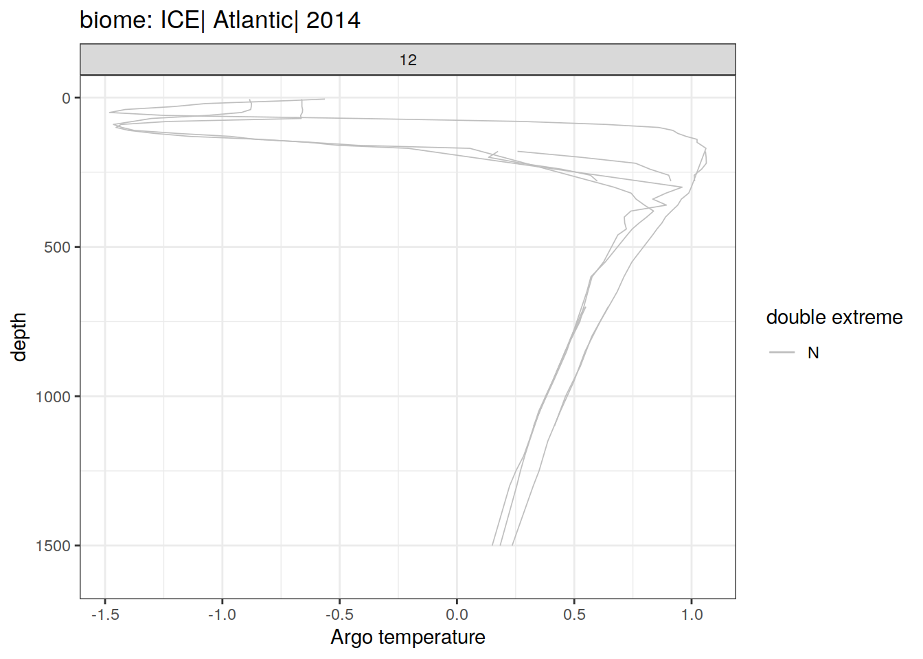
[[2]]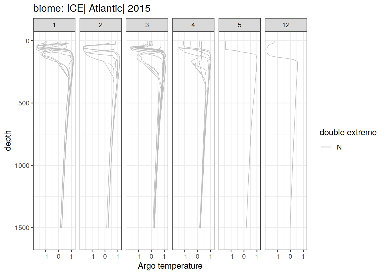
[[3]]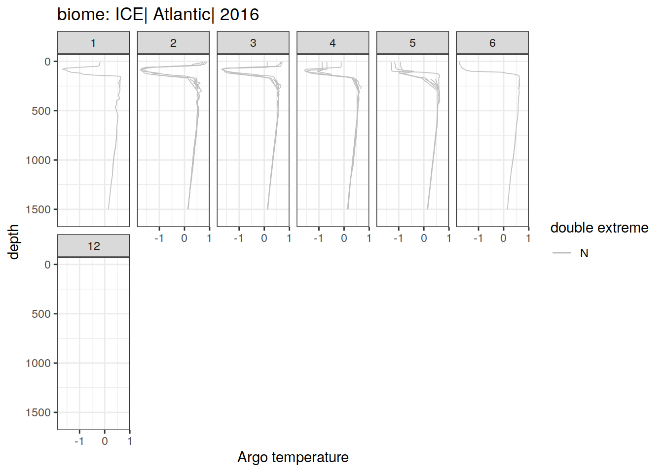
[[4]]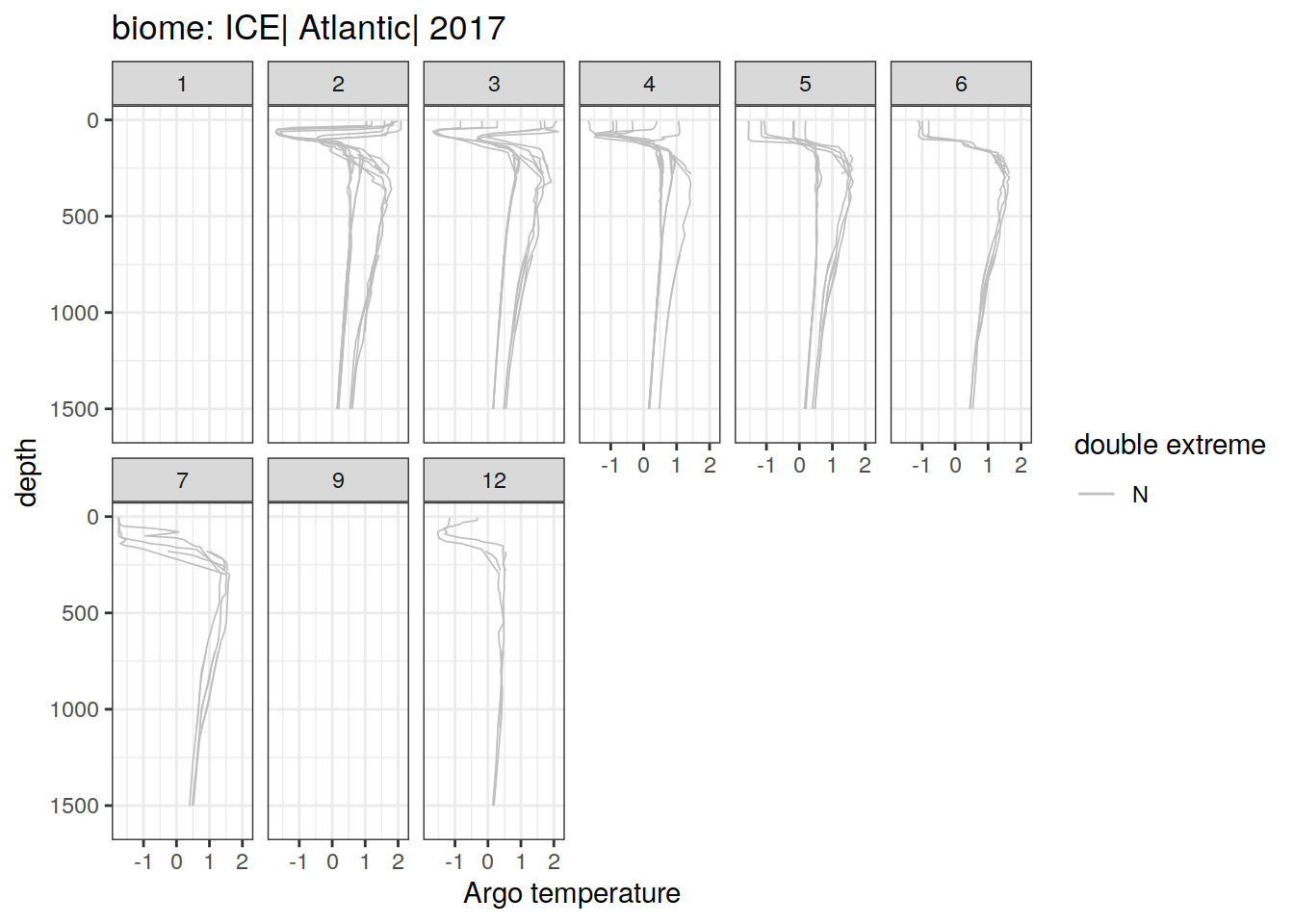
[[5]]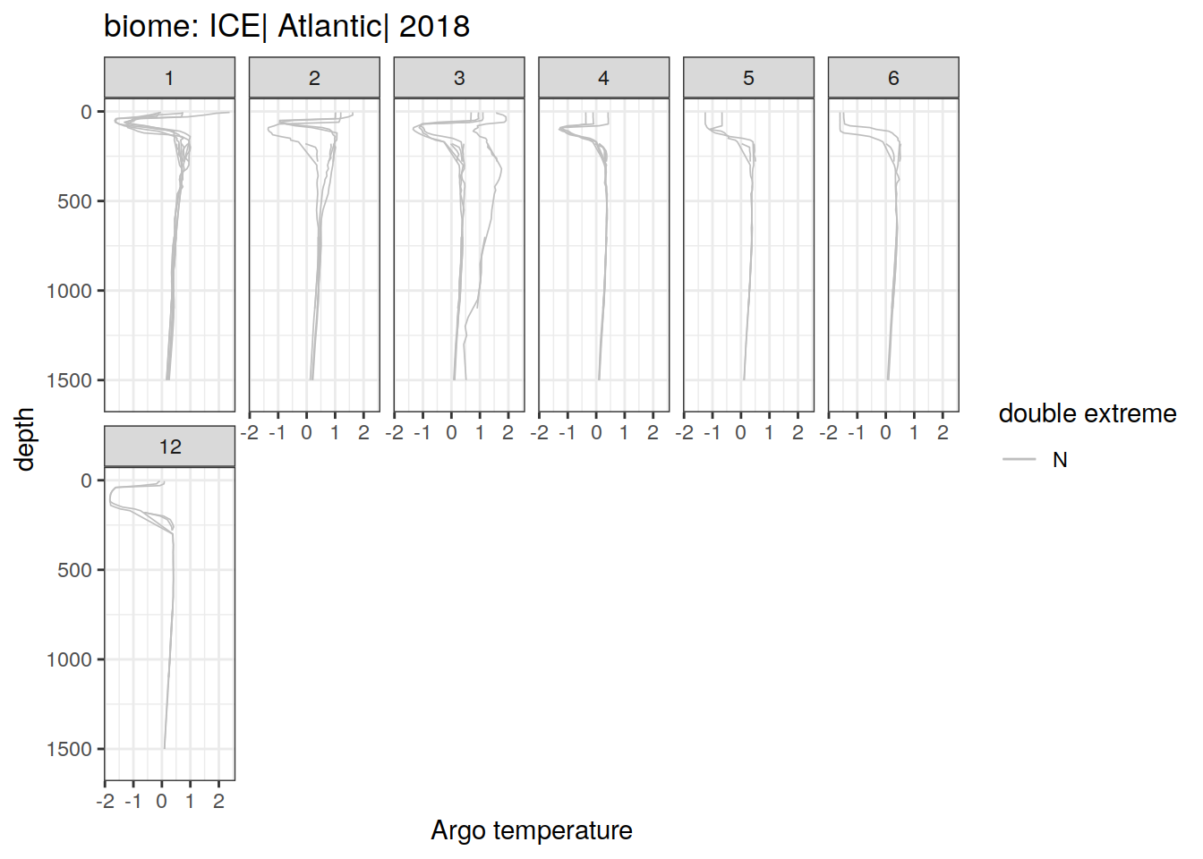
[[6]]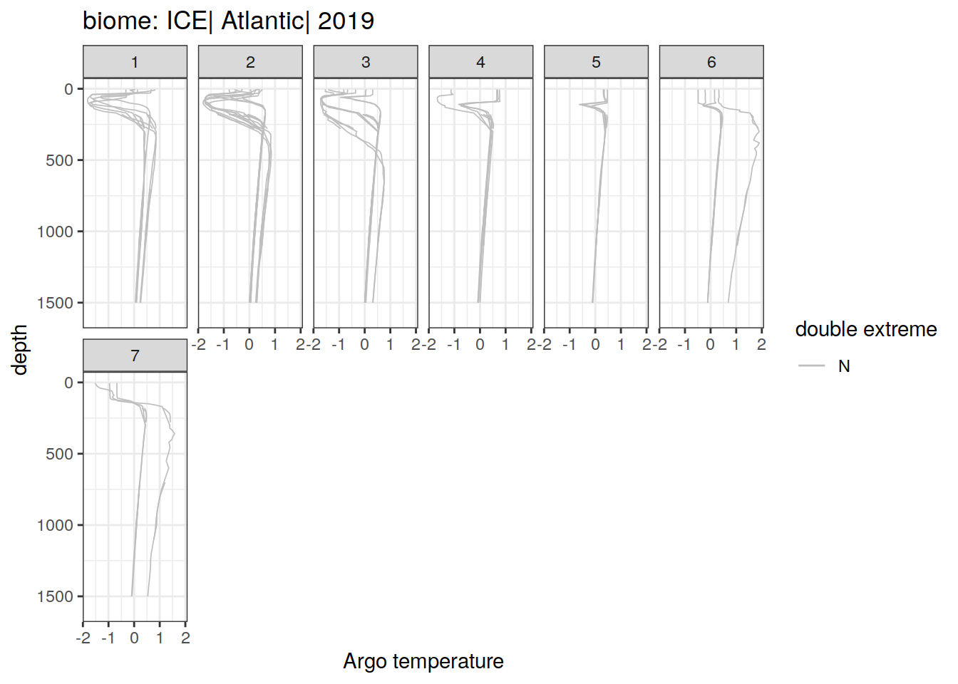
[[7]]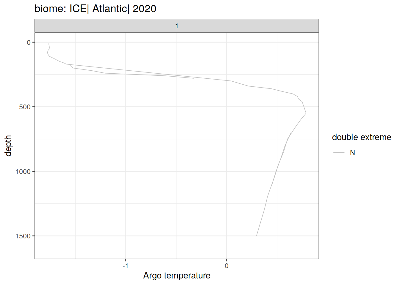
[[8]]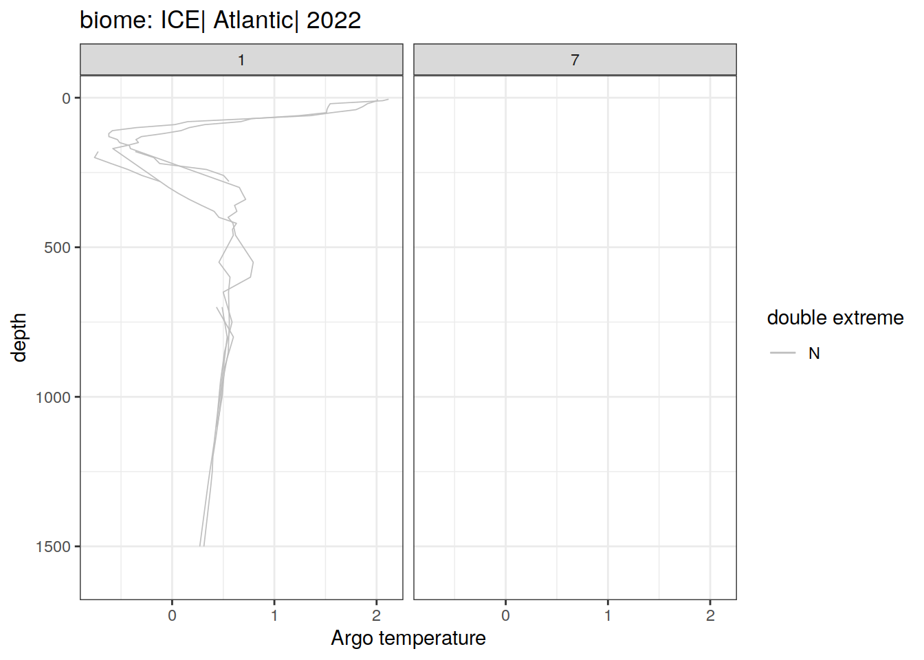
[[9]]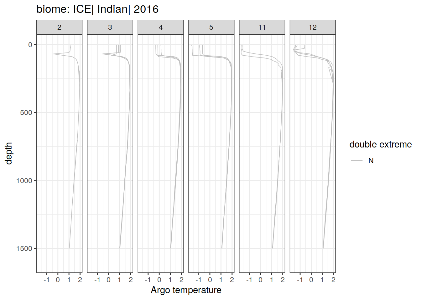
[[10]]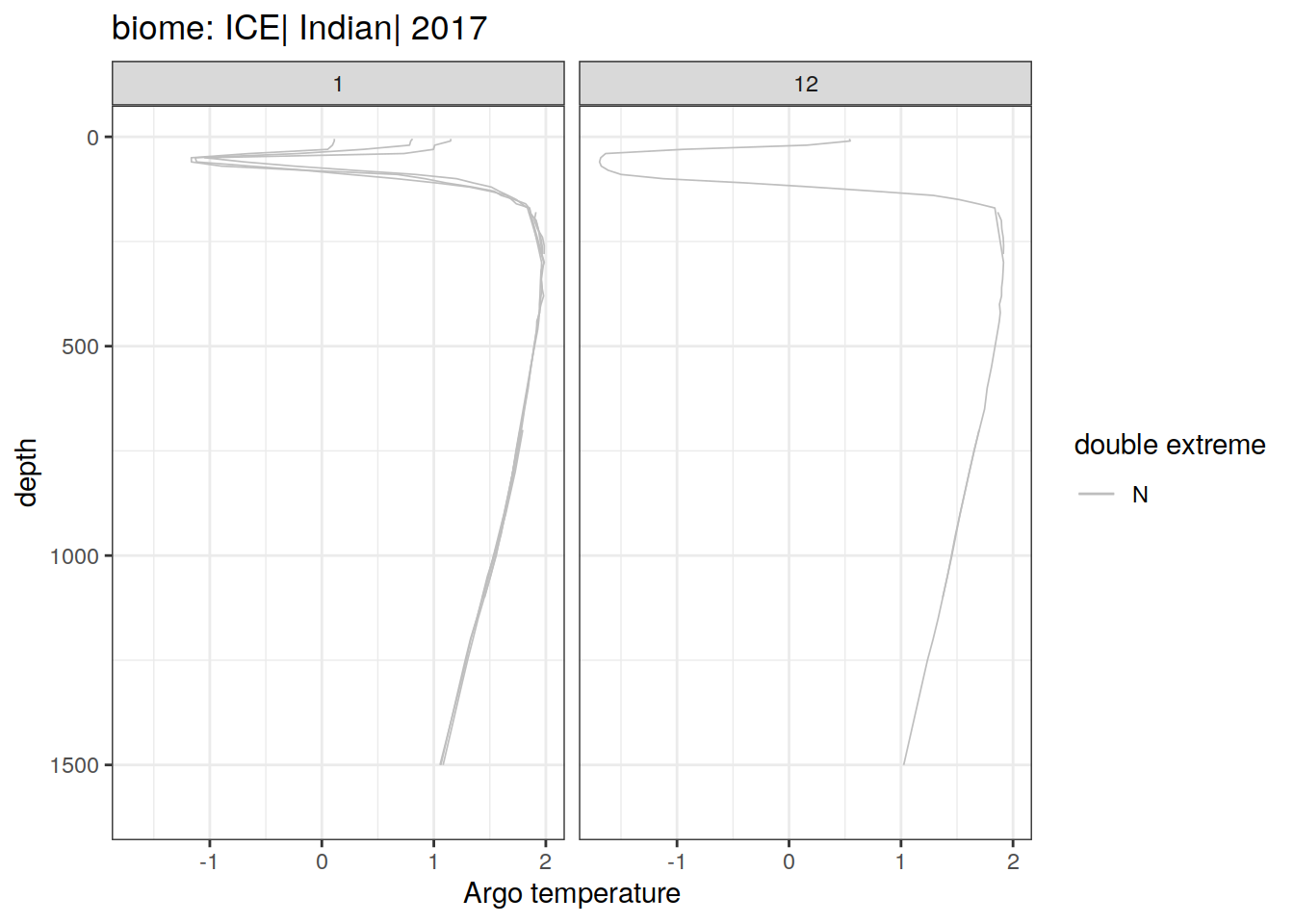
[[11]]
[[12]]
[[13]]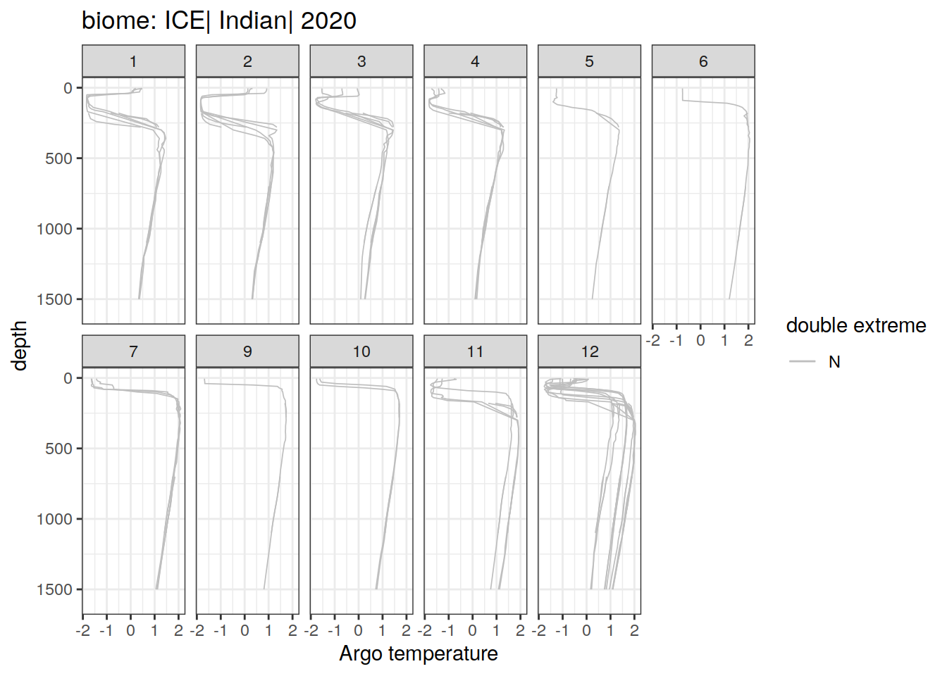
[[14]]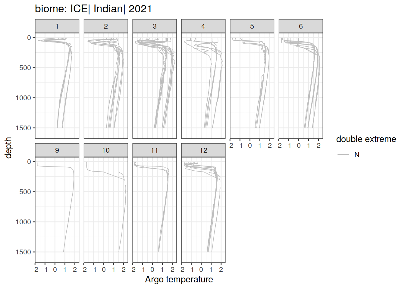
[[15]]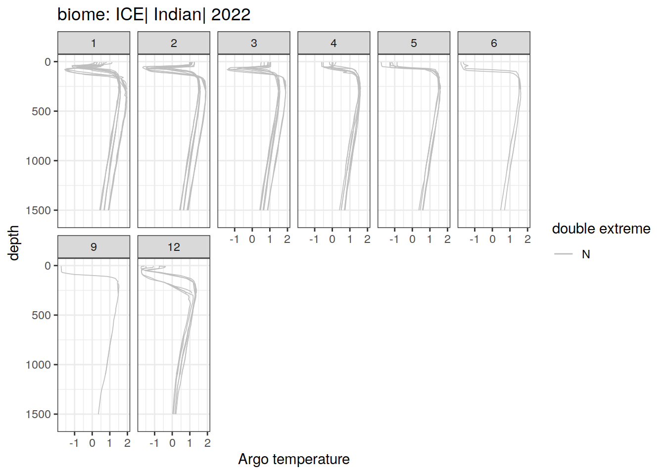
[[16]]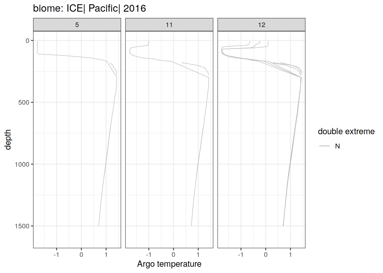
[[17]]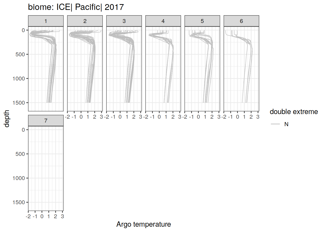
[[18]]
[[19]]
[[20]]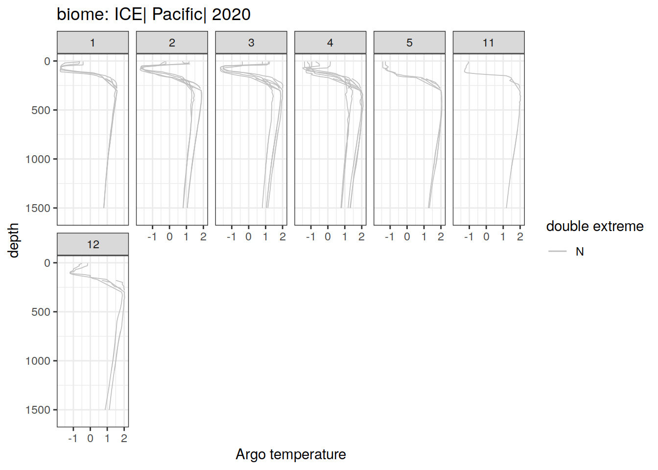
[[21]]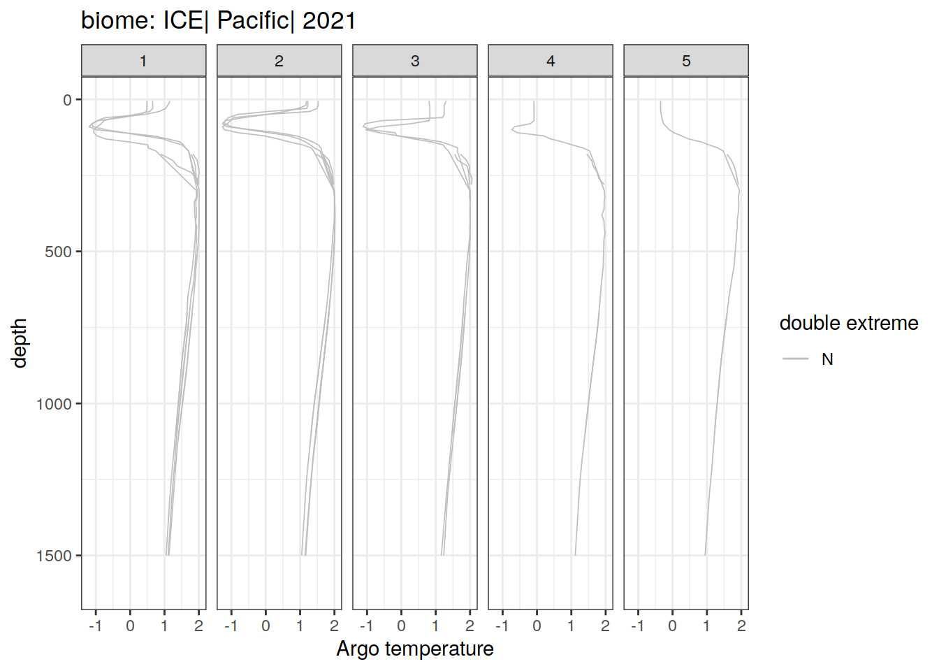
[[22]]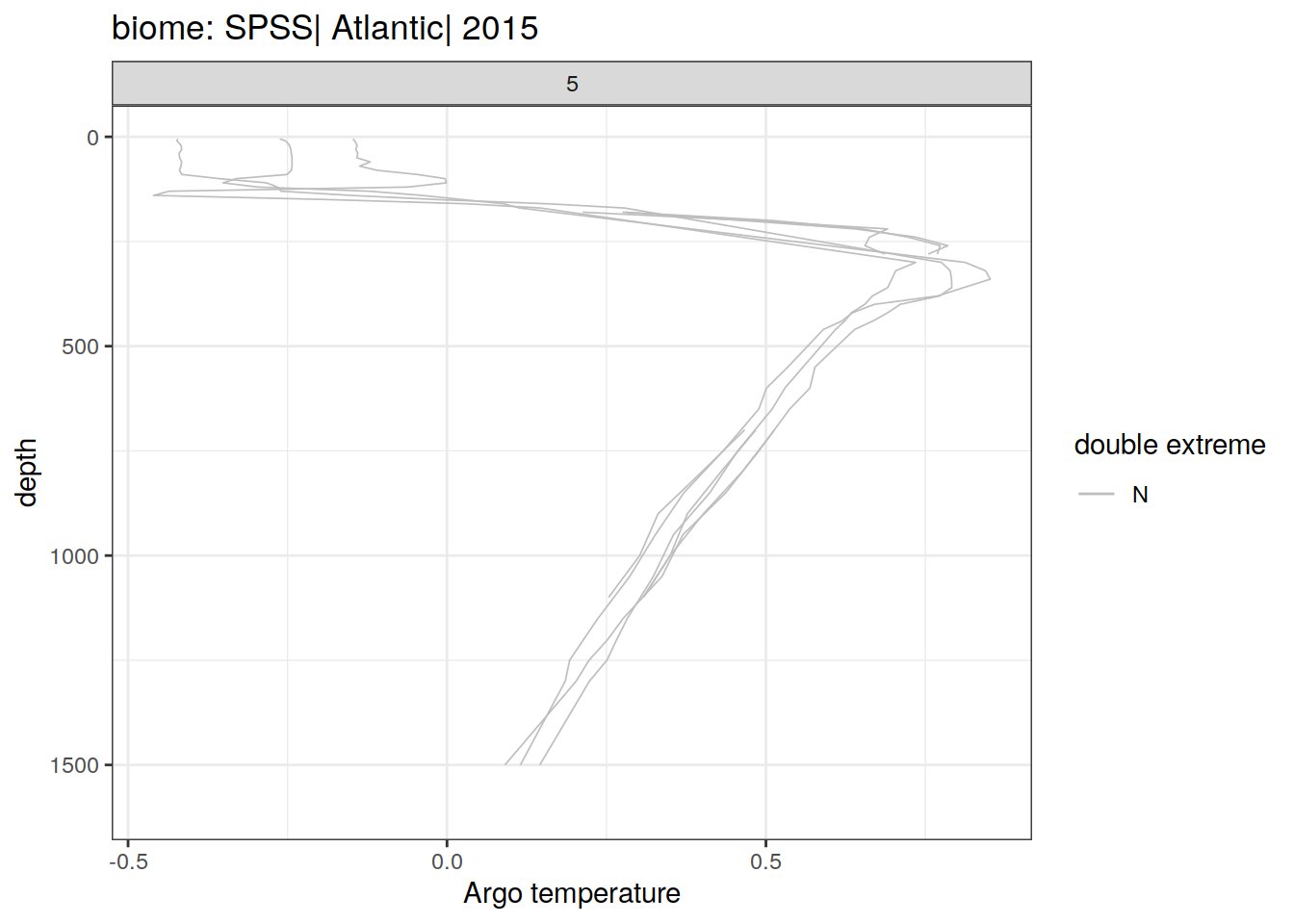
[[23]]
[[24]]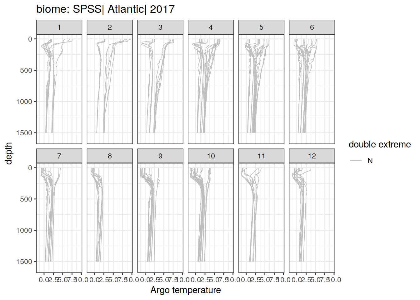
[[25]]
[[26]]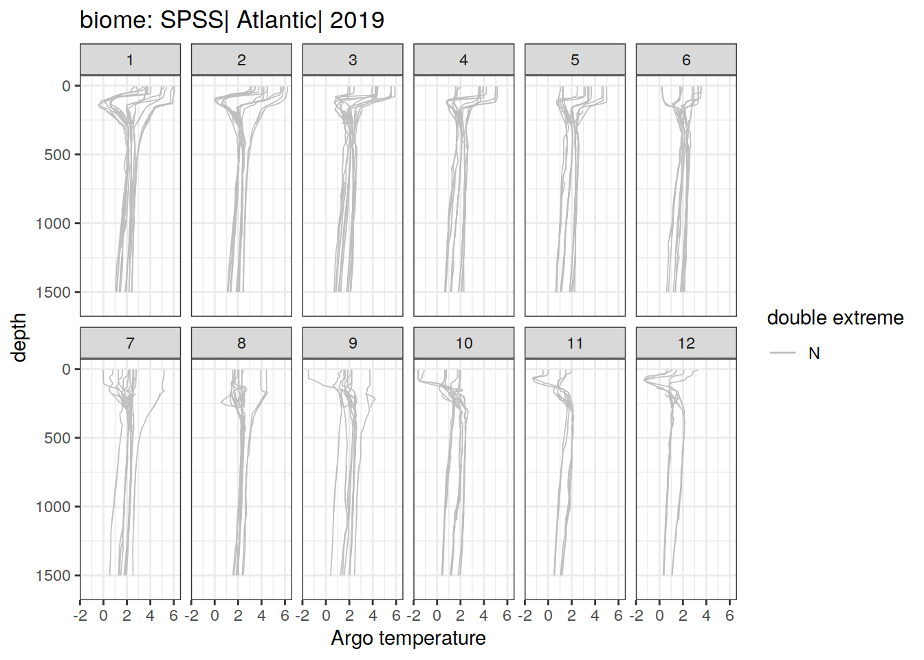
[[27]]
[[28]]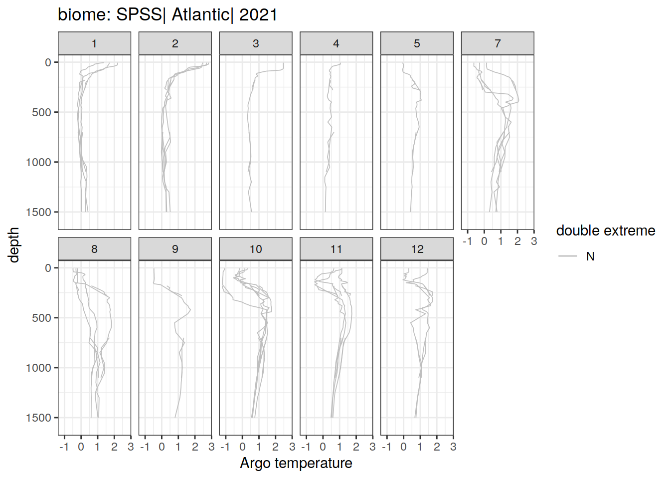
[[29]]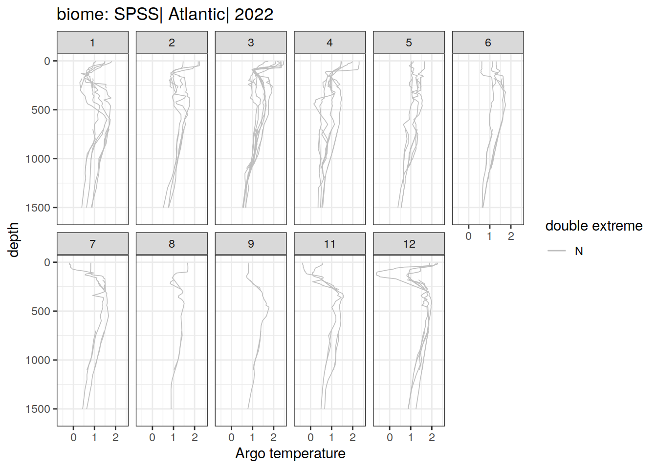
[[30]]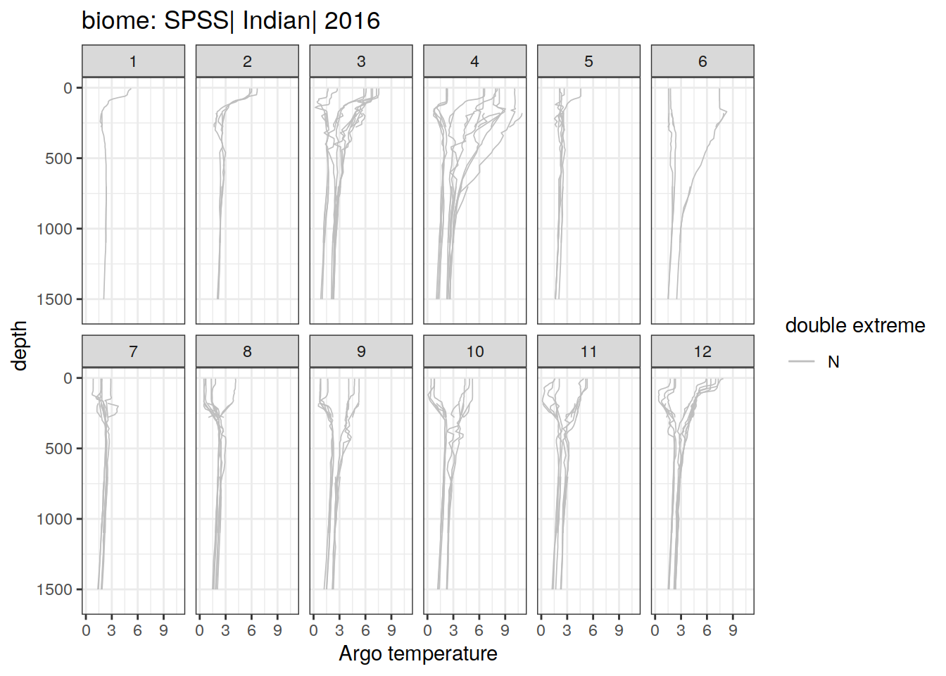
[[31]]
[[32]]
[[33]]
[[34]]
[[35]]
[[36]]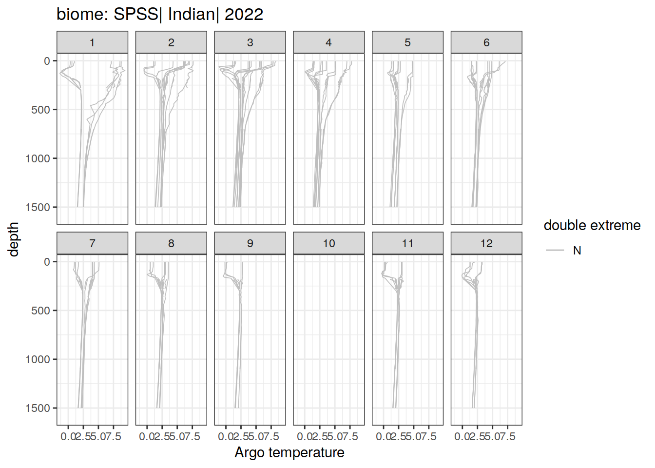
[[37]]
[[38]]
[[39]]
[[40]]
[[41]]
[[42]]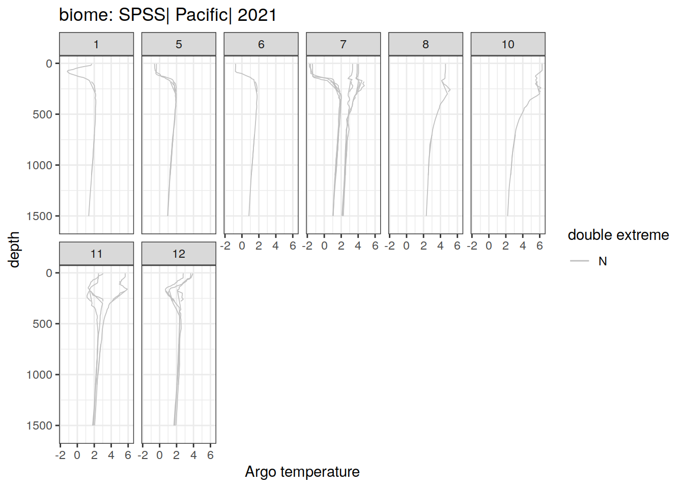
[[43]]
[[44]]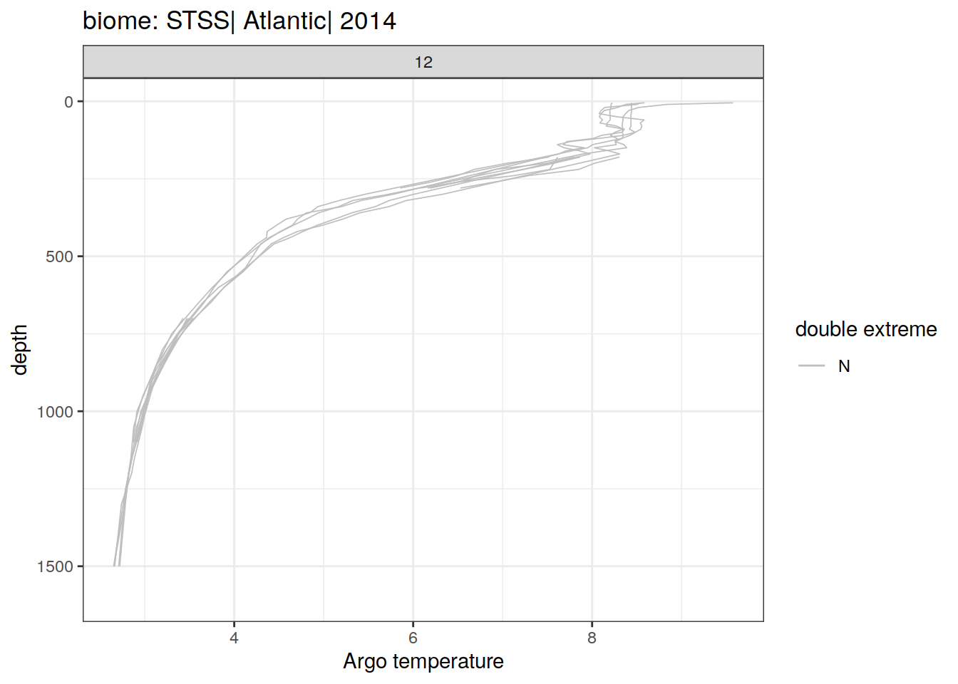
[[45]]
[[46]]
[[47]]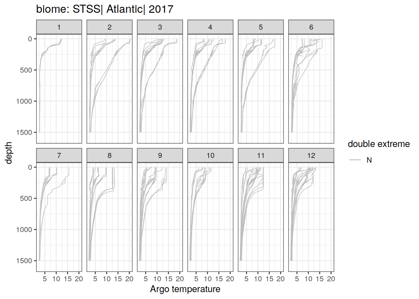
[[48]]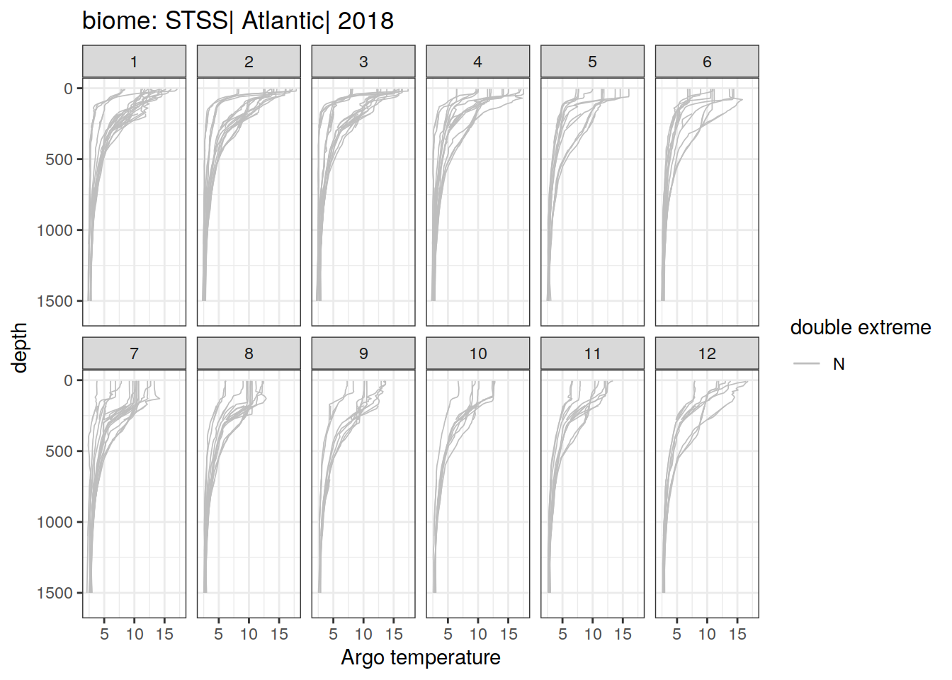
[[49]]
[[50]]
[[51]]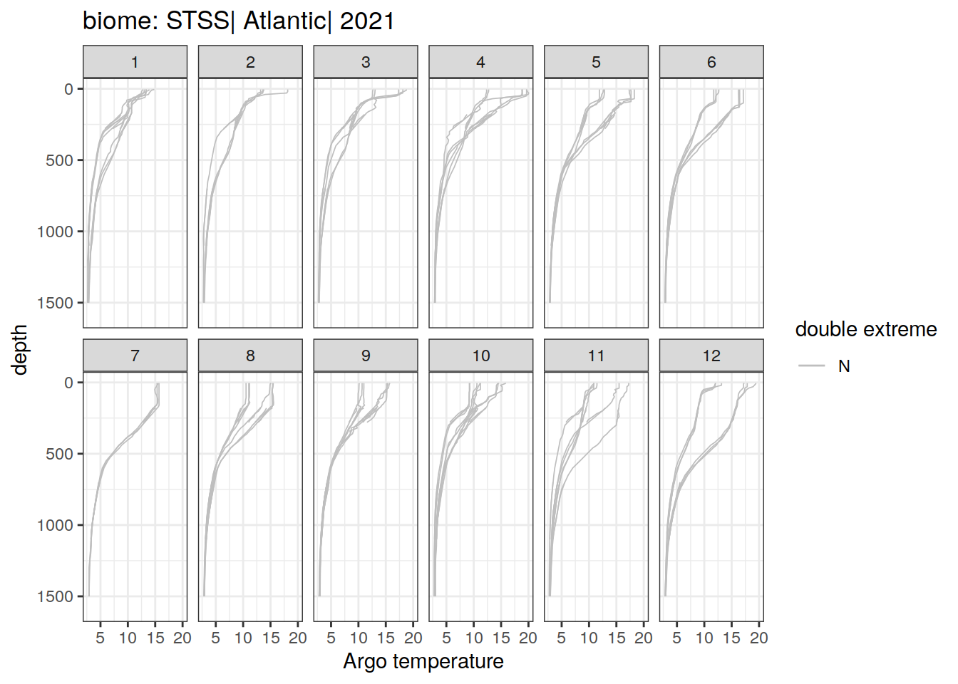
[[52]]
[[53]]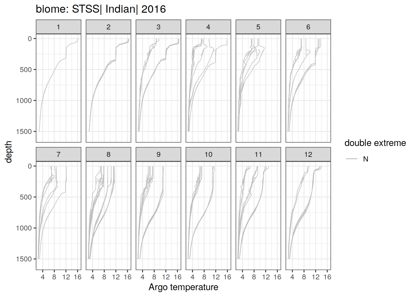
[[54]]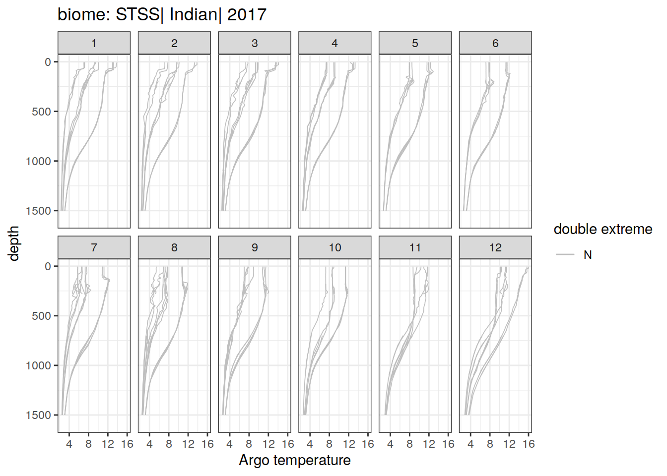
[[55]]
[[56]]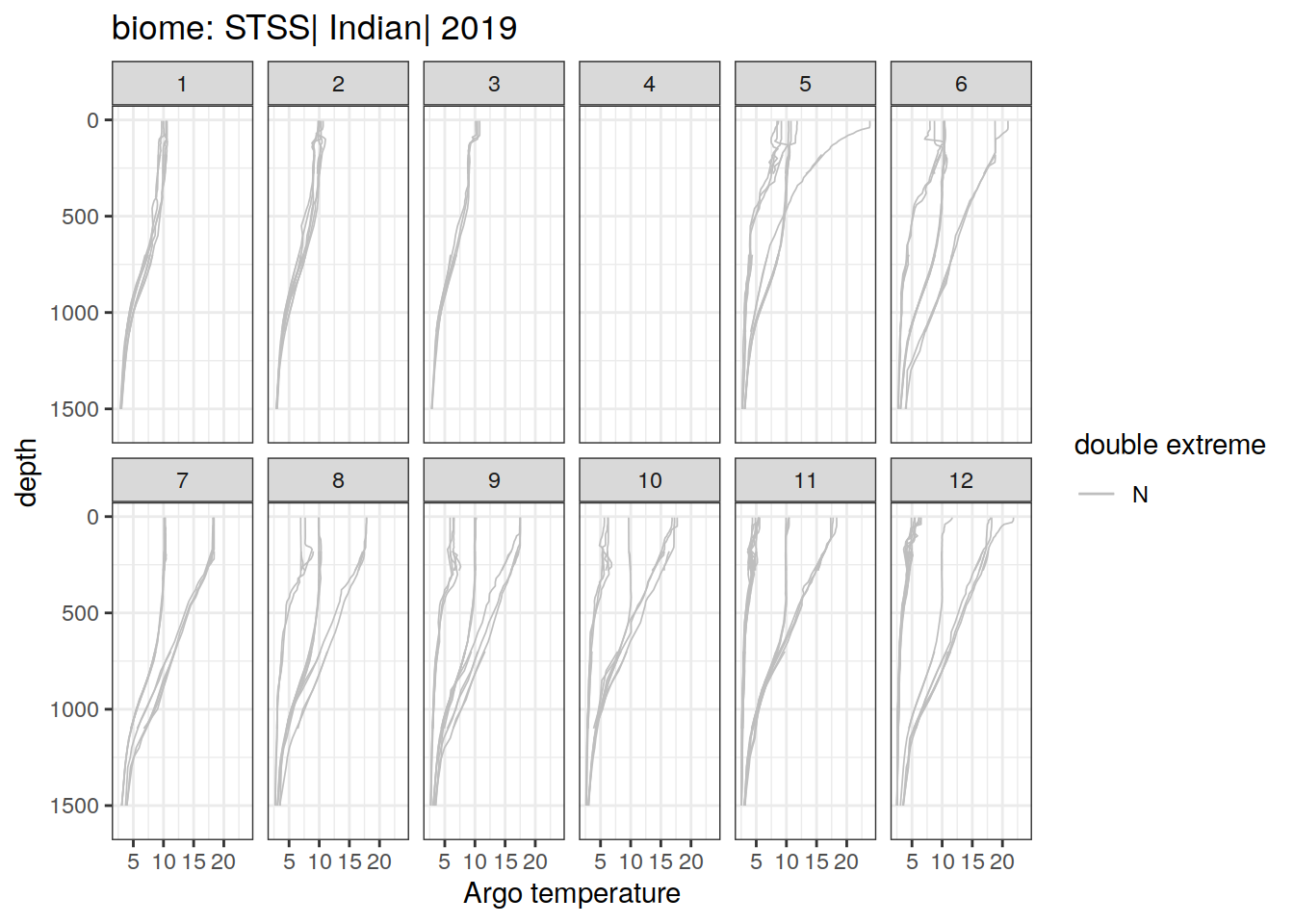
[[57]]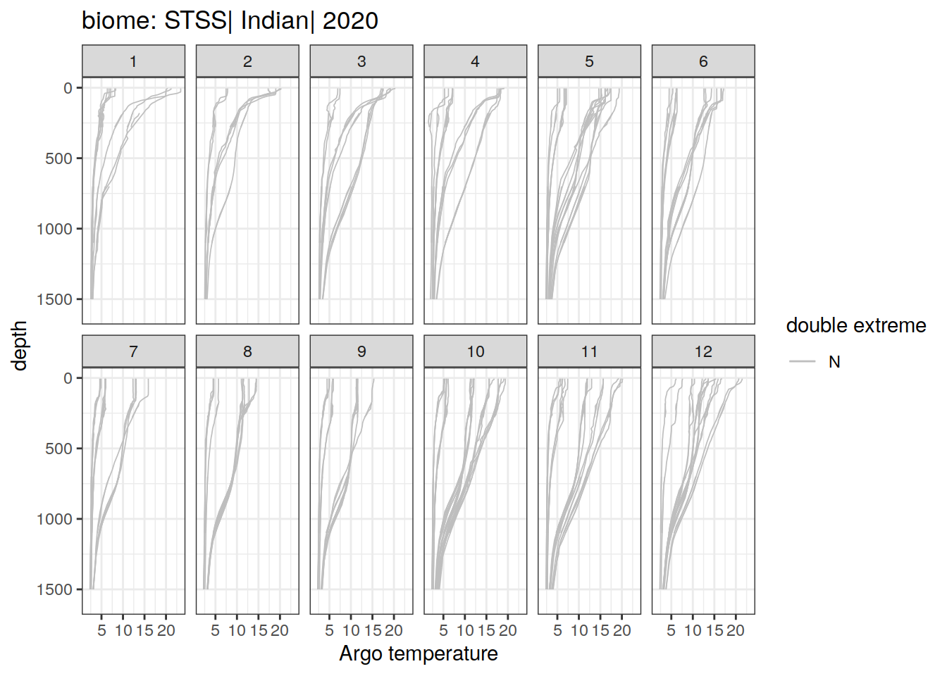
[[58]]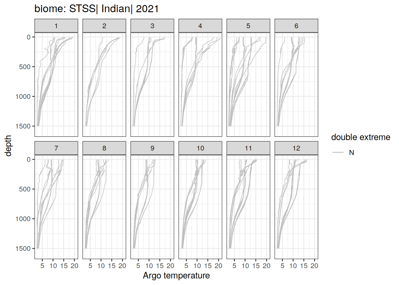
[[59]]
[[60]]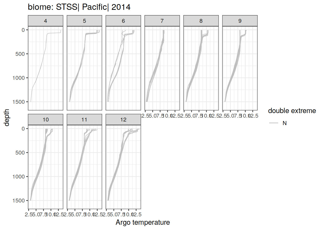
[[61]]
[[62]]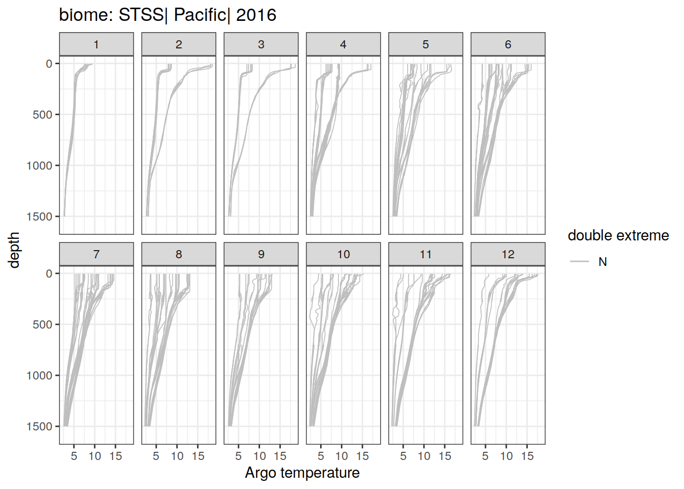
[[63]]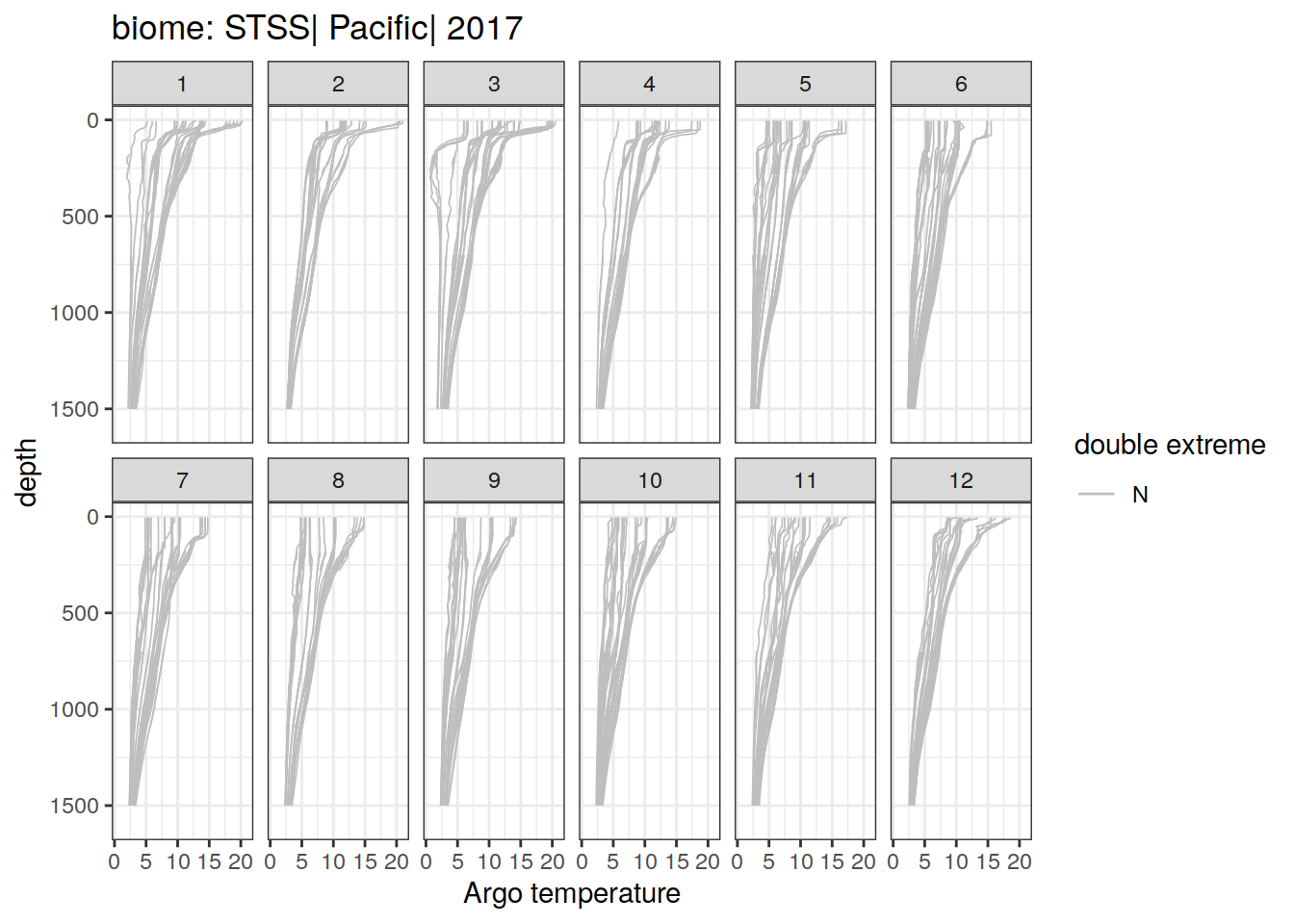
[[64]]
[[65]]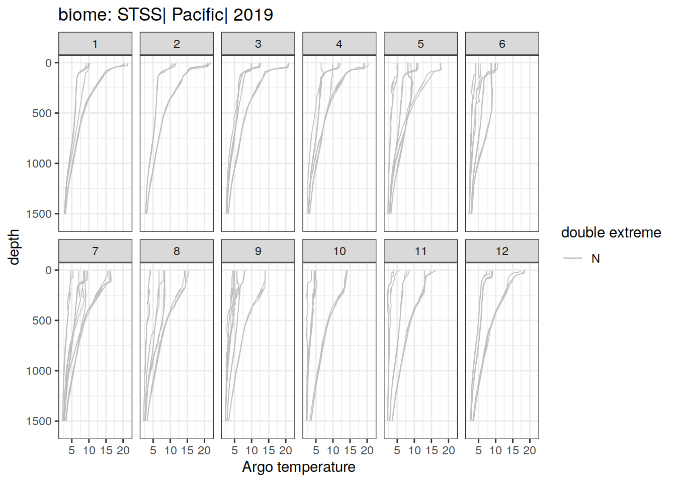
[[66]]
[[67]]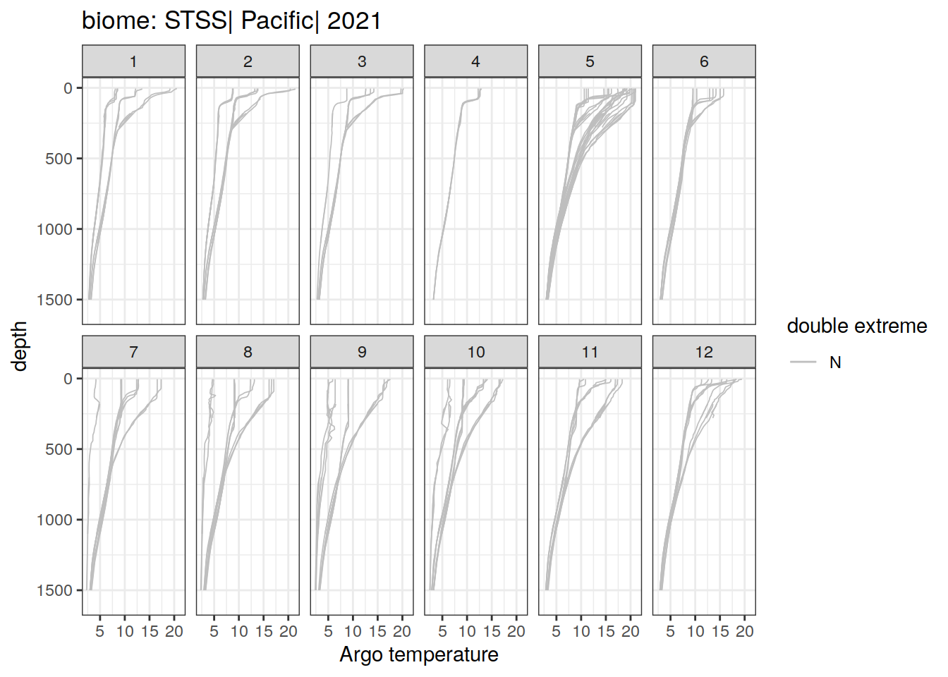
[[68]]
Pacific basin, STSS biome, December 2017
Pacific_STSS_2017 <- profile_double_extreme %>%
  filter(date == '2017-12-15',
         basin_AIP == 'Pacific',
         biome_name == 'STSS')

# pH:
Pacific_STSS_2017 %>%
  ggplot()+
  geom_path(data = Pacific_STSS_2017 %>% filter(double_extreme == 'N'),
            aes(x = pH,
                y = depth,
                group = file_id,
                col = double_extreme),
            size = 0.3)+
  geom_path(data = Pacific_STSS_2017 %>% filter(double_extreme == 'E'),
            aes(x = pH,
                y = depth,
                group = file_id,
                col = double_extreme),
            size = 0.5)+
  scale_y_reverse()+
  scale_color_manual(values = c('E' = 'red', 'N' = 'grey'))+
  labs(title = 'Pacific, STSS biome, December 2017',
       col = 'double extreme',
       x = 'Argo pH',
       y = 'depth')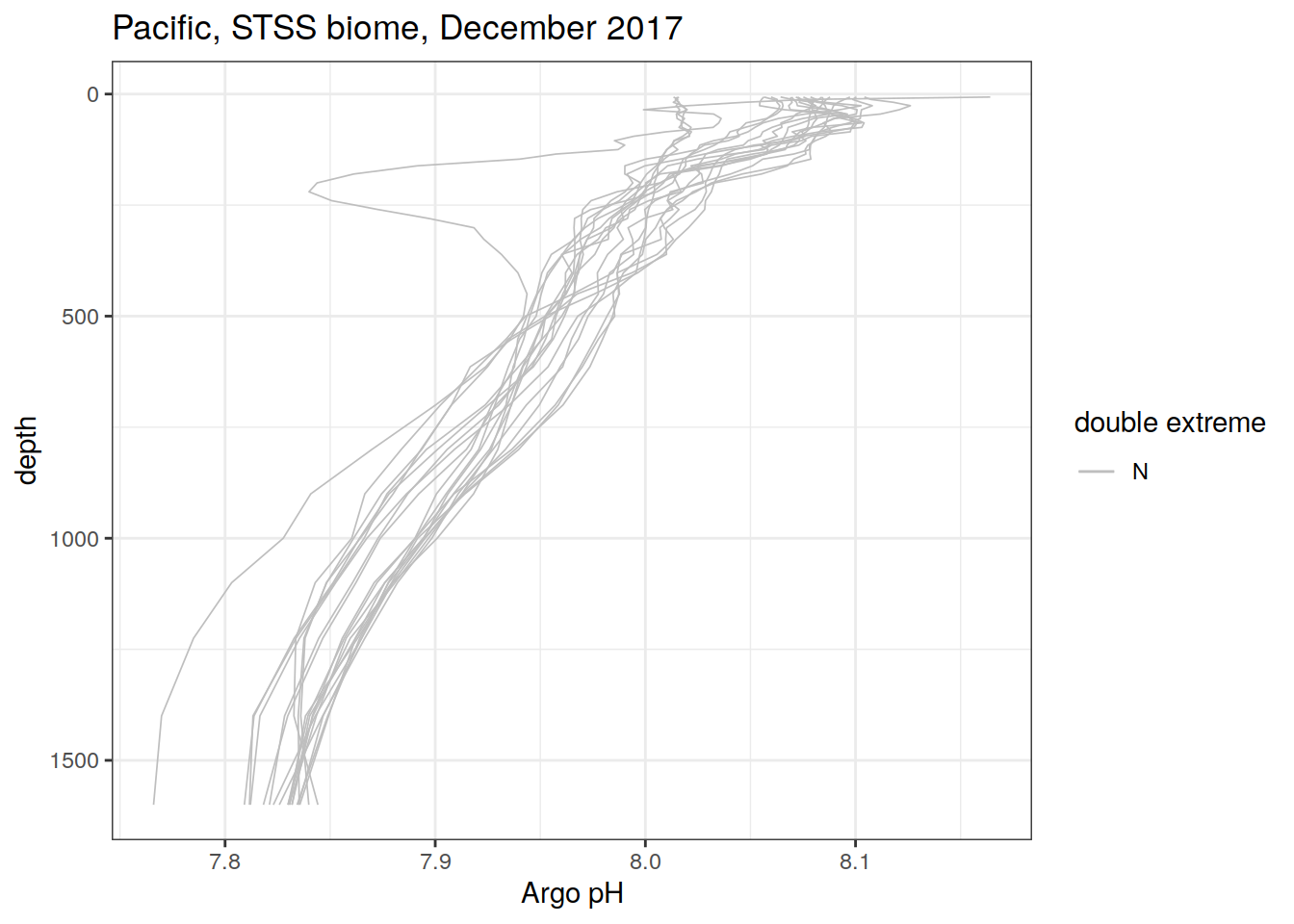
# Temperature

Pacific_STSS_2017 %>%
  ggplot()+
  geom_path(data = Pacific_STSS_2017 %>% filter(double_extreme == 'N'),
            aes(x = temp,
                y = depth,
                group = file_id,
                col = double_extreme),
            size = 0.3)+
  geom_path(data = Pacific_STSS_2017 %>% filter(double_extreme == 'E'),
            aes(x = temp,
                y = depth,
                group = file_id,
                col = double_extreme),
            size = 0.5)+
  scale_y_reverse()+
  scale_color_manual(values = c('E' = 'red', 'N' = 'grey'))+
  labs(title = 'Pacific, STSS biome, December 2017',
       col = 'double extreme',
       x = 'Argo pH',
       y = 'depth')
rm(Pacific_STSS_2017)Pacific basin, STSS biome, December 2019
No profiles for December 2019 in SPSS or STSS Pacific
sessionInfo()R version 4.2.2 (2022-10-31)
Platform: x86_64-pc-linux-gnu (64-bit)
Running under: openSUSE Leap 15.5
Matrix products: default
BLAS: /usr/local/R-4.2.2/lib64/R/lib/libRblas.so
LAPACK: /usr/local/R-4.2.2/lib64/R/lib/libRlapack.so
locale:
[1] LC_CTYPE=en_US.UTF-8 LC_NUMERIC=C
[3] LC_TIME=en_US.UTF-8 LC_COLLATE=en_US.UTF-8
[5] LC_MONETARY=en_US.UTF-8 LC_MESSAGES=en_US.UTF-8
[7] LC_PAPER=en_US.UTF-8 LC_NAME=C
[9] LC_ADDRESS=C LC_TELEPHONE=C
[11] LC_MEASUREMENT=en_US.UTF-8 LC_IDENTIFICATION=C
attached base packages:
[1] stats graphics grDevices utils datasets methods base
other attached packages:
[1] ggnewscale_0.4.8 lubridate_1.9.0 timechange_0.1.1 forcats_0.5.2
[5] stringr_1.5.0 dplyr_1.1.3 purrr_1.0.2 readr_2.1.3
[9] tidyr_1.3.0 tibble_3.2.1 ggplot2_3.4.4 tidyverse_1.3.2
[13] workflowr_1.7.0
loaded via a namespace (and not attached):
[1] Rcpp_1.0.10 getPass_0.2-2 ps_1.7.2
[4] assertthat_0.2.1 rprojroot_2.0.3 digest_0.6.30
[7] utf8_1.2.2 R6_2.5.1 cellranger_1.1.0
[10] backports_1.4.1 reprex_2.0.2 evaluate_0.18
[13] highr_0.9 httr_1.4.4 pillar_1.9.0
[16] rlang_1.1.1 readxl_1.4.1 googlesheets4_1.0.1
[19] rstudioapi_0.15.0 whisker_0.4 callr_3.7.3
[22] jquerylib_0.1.4 rmarkdown_2.18 labeling_0.4.2
[25] googledrive_2.0.0 munsell_0.5.0 broom_1.0.5
[28] compiler_4.2.2 httpuv_1.6.6 modelr_0.1.10
[31] xfun_0.35 pkgconfig_2.0.3 htmltools_0.5.8.1
[34] tidyselect_1.2.0 fansi_1.0.3 crayon_1.5.2
[37] withr_2.5.0 tzdb_0.3.0 dbplyr_2.2.1
[40] later_1.3.0 grid_4.2.2 jsonlite_1.8.3
[43] gtable_0.3.1 lifecycle_1.0.3 DBI_1.2.2
[46] git2r_0.30.1 magrittr_2.0.3 scales_1.2.1
[49] cli_3.6.1 stringi_1.7.8 cachem_1.0.6
[52] farver_2.1.1 fs_1.5.2 promises_1.2.0.1
[55] xml2_1.3.3 bslib_0.4.1 ellipsis_0.3.2
[58] generics_0.1.3 vctrs_0.6.4 tools_4.2.2
[61] glue_1.6.2 hms_1.1.2 processx_3.8.0
[64] fastmap_1.1.0 yaml_2.3.6 colorspace_2.0-3
[67] gargle_1.2.1 rvest_1.0.3 knitr_1.41
[70] haven_2.5.1 sass_0.4.4