Marine Heat Waves anomaly profiles
Marguerite Larriere & Jens Daniel Müller
06 June, 2024
Last updated: 2024-06-06
Checks: 7 0
Knit directory:
bgc_argo_r_argodata/analysis/
This reproducible R Markdown analysis was created with workflowr (version 1.7.0). The Checks tab describes the reproducibility checks that were applied when the results were created. The Past versions tab lists the development history.
Great! Since the R Markdown file has been committed to the Git repository, you know the exact version of the code that produced these results.
Great job! The global environment was empty. Objects defined in the global environment can affect the analysis in your R Markdown file in unknown ways. For reproduciblity it’s best to always run the code in an empty environment.
The command set.seed(20211008) was run prior to running
the code in the R Markdown file. Setting a seed ensures that any results
that rely on randomness, e.g. subsampling or permutations, are
reproducible.
Great job! Recording the operating system, R version, and package versions is critical for reproducibility.
Nice! There were no cached chunks for this analysis, so you can be confident that you successfully produced the results during this run.
Great job! Using relative paths to the files within your workflowr project makes it easier to run your code on other machines.
Great! You are using Git for version control. Tracking code development and connecting the code version to the results is critical for reproducibility.
The results in this page were generated with repository version f35ae7a. See the Past versions tab to see a history of the changes made to the R Markdown and HTML files.
Note that you need to be careful to ensure that all relevant files for
the analysis have been committed to Git prior to generating the results
(you can use wflow_publish or
wflow_git_commit). workflowr only checks the R Markdown
file, but you know if there are other scripts or data files that it
depends on. Below is the status of the Git repository when the results
were generated:
Ignored files:
    Ignored:    .RData
    Ignored:    .Rproj.user/

Untracked files:
    Untracked:  analysis/draft.Rmd
    Untracked:  load_argo_core_output.txt
    Untracked:  poster_profile_argo.png

Unstaged changes:
    Modified:   analysis/CESM_comparison.Rmd
    Deleted:    analysis/MHWs_categorisation.Rmd
    Modified:   analysis/_site.yml
    Modified:   analysis/anomaly_SST_2023.Rmd
    Modified:   analysis/child/cluster_analysis_base.Rmd
    Modified:   analysis/coverage_maps_North_Atlantic.Rmd
    Modified:   analysis/load_broullon_DIC_TA_clim.Rmd
    Modified:   analysis/temp_core_align_climatology.Rmd
    Modified:   code/Workflowr_project_managment.R
    Modified:   code/start_background_job.R
    Modified:   code/start_background_job_load.R
    Modified:   code/start_background_job_partial.R
Note that any generated files, e.g. HTML, png, CSS, etc., are not included in this status report because it is ok for generated content to have uncommitted changes.
These are the previous versions of the repository in which changes were
made to the R Markdown (analysis/MHWs_vertical_anomaly.Rmd)
and HTML (docs/MHWs_vertical_anomaly.html) files. If you’ve
configured a remote Git repository (see ?wflow_git_remote),
click on the hyperlinks in the table below to view the files as they
were in that past version.
| File | Version | Author | Date | Message |
|---|---|---|---|---|
| Rmd | f35ae7a | mlarriere | 2024-06-06 | cleaning code |
| html | 2d63792 | mlarriere | 2024-05-24 | Build site. |
| Rmd | a4c7c05 | mlarriere | 2024-05-24 | Absolute maximum anomalies categorisation |
| Rmd | cebda03 | mlarriere | 2024-05-22 | Hovmoeller plot |
| html | 3ac87c9 | mlarriere | 2024-05-20 | Build site. |
| Rmd | 5304024 | mlarriere | 2024-05-20 | choosing extent |
| html | b0fb164 | mlarriere | 2024-05-16 | Build site. |
| Rmd | fbf0c64 | mlarriere | 2024-05-16 | latitude, longitude and day of the month graphs |
| html | 22e0206 | mlarriere | 2024-05-16 | Build site. |
| Rmd | d0f58b6 | mlarriere | 2024-05-16 | latitude, longitude and day of the month graphs |
| html | 96d4b76 | mlarriere | 2024-05-14 | Build site. |
| Rmd | 91e6028 | mlarriere | 2024-05-13 | adding subsection CESM comparison |
| html | af6594f | mlarriere | 2024-05-13 | Build site. |
| Rmd | 30f9250 | mlarriere | 2024-05-13 | Adding CESM subsection |
Task
Focusing on 2023 Only core Argo - focus on temperature anomalies
Dependencies
temp_core_va.rds - temperature of core argo floats after vertical alignment for a given year.
core_metadata.rds - file with metadata concerning the floats such as platform number, cycle number, date, lat, lon and quality control results.
temp_anomaly_va.rds - file containing the temperature anomalies (temp core - climatology).
SST_anomaly2023_NorthAtlantic_clim2004.rds - file containing SST anomalies for each lat, lon, month on a 1°x1° grid. Data from the SOM-FFN model with same climatology than Argo, i.e. 2004-2019.
Outputs
path_emlr_utilities <- "/nfs/kryo/work/jenmueller/emlr_cant/utilities/files/"
path_basin_mask <- "/nfs/kryo/work/datasets/gridded/ocean/interior/reccap2/supplementary/"
path_argo <- '/nfs/kryo/work/datasets/ungridded/3d/ocean/floats/bgc_argo'
path_argo_core <- '/nfs/kryo/work/datasets/ungridded/3d/ocean/floats/core_argo_r_argodata_2024-03-13'

path_argo_core_preprocessed <- paste0(path_argo_core, "/preprocessed_core_data")

path_mhw<- '/net/kryo/work/datasets/gridded/ocean/2d/obs/mhw'
#Area of interest: North Atlantic north west - lat:(60,30), lon:(-70,-30), North Atlantic east - lat:(0,40), lon:(-30,0)
chosen_extent <- list(
lat_min = 0, #30
lat_max = 40, #60
lon_min = -30, #-70
lon_max = 0 #-30
)
name_extent<- "East" #Northwest
#base map for the plots
world_coordinates <- map_data("world")
#year of interest
target_year<-2023Load data
Load biomes
#---------------- Biomes ----------------
#Load biome separations
region_masks_all <-
  stars::read_ncdf(paste(
    path_basin_mask, "RECCAP2_region_masks_all_v20221025.nc", sep = "")) %>%
  as_tibble() %>%
  mutate(seamask = as.factor(seamask))

region_masks_all <- region_masks_all %>%
  mutate(lon = ifelse(lon > 180, lon - 360, lon)) %>% #shift longitude to be in range (-180°, 180°) for better vizualisation
  pivot_longer(open_ocean:atlantic,
               names_to = 'region',
               values_to = 'value') %>%
  mutate(value = as.factor(value))

#Biomes North Atlantic
region_masks_atlantic <- region_masks_all %>%
  filter(region == 'atlantic',
         value != 0) %>%
  mutate(coast = as.character(coast))

biomes_atlantic <- region_masks_atlantic %>%
  filter(value %in% c(1,2,3))

biomes_subset <- biomes_atlantic %>%
  select(lat, lon, biome_value = value)

biomes_names<-c("SPSS", "STSS", "STPS")

ggplot()+
  geom_map(data = world_coordinates, map = world_coordinates, aes(long, lat, map_id = region), fill = "grey") + #base map
  lims(x= c(-100, 50), y = c(0, 80))+ #North Atlantic
  coord_quickmap(expand = 0) +
  geom_tile(data = biomes_atlantic,   aes(x = lon,  y = lat,  fill = value))+
  scale_fill_manual(values = c("1" = "cadetblue", "2" = "azure", "3" = "lightskyblue3"),
                    labels = biomes_names) +
  labs(title = 'Biomes - North Atlantic basin',
       subtitle = 'RECCAP data',
         x = "longitude", y = "latitude", fill = "Biomes") +
  theme(plot.title = element_text(size = 16),
        plot.subtitle = element_text(size = 12),
        legend.text = element_text(size = 10),
        legend.title = element_text(size = 12, face = "bold"),
        legend.key.width = unit(0.5, "cm"),
        legend.key.height = unit(2, "cm"))
Load Argo floats data
Load SST anomaly
#Read SST anomaly, computed using climatology:2009-2019 (from anomaly_SST_2023.Rmd)
sst_anomaly_northAtlantic<- read_rds(paste(path_argo_core_preprocessed, "/SST_anomaly2023_NorthAtlantic_clim2004-2019.rds", sep = ""))
Argo floats
Distribution over North Atlantic basin
#Histogram -- number of floats per month and biome
unique_platforms_per_month <- core_anomaly_with_platform_2023 %>%
   group_by(month) %>%
  filter(lat>0, lat<70, lon>-80, lon<0) %>%
   summarize(unique_platforms = n_distinct(platform_number))


ggplot(unique_platforms_per_month, aes(x = factor(month), y = unique_platforms)) +
    geom_bar(stat = "identity", fill = "lightskyblue3",color = "black", size = 0.25) +
    labs(title = "Amount of platform per month, in North Atlantic, 2023",
         x = "Months", y = "Number of argo floats", fill = "Biomes") +
    theme_minimal() +
    guides(fill = FALSE)
    # scale_fill_manual(values = c("1" = "#1034A6", "2" = "#f59c04", "3" = "darkred"), labels = c("1" = "SPSS", "2" = "STSS", "3" = "STPS")) +

#Number of cycle per platform
cycle_counts <- core_anomaly_with_platform_2023 %>%
  group_by(platform_number) %>%
  summarise(cycle_count = n_distinct(cycle_number))
print(cycle_counts)
# A tibble: 4,621 × 2
platform_number cycle_count
<chr> <int>
1 1901443 14
2 1901514 34
3 1901604 5
4 1901701 37
5 1901711 31
6 1901727 38
7 1901728 26
8 1901730 37
9 1901731 37
10 1901732 37
# ℹ 4,611 more rows#Join the SST anomaly with the core Argo anomaly profiles
core_anomaly_with_platform_2023<-core_anomaly_with_platform_2023 %>%
filter(!is.na(depth)) %>%
select(-profile_range, -day_of_year)
complete_anomaly_profile<- core_anomaly_with_platform_2023 %>%
inner_join(sst_anomaly_northAtlantic, by = c("lat", "lon", "month"))
#---Chosen subset
core_anomaly_2023_natlantic_subset<- complete_anomaly_profile %>%
filter(lat > chosen_extent$lat_min, lat < chosen_extent$lat_max,
lon > chosen_extent$lon_min, lon < chosen_extent$lon_max) %>%
select(-interpolated_temp) Distribution over East-North Atlantic
Using the SST map computed in “anomaly_SST_2023.Rmd” and ClimateReanalyser, we identify 1 area of particular interest for SST anomalies in 2023 in the North Atlantic Ocean: The East coast of the North Atlantic Ocean, where the SST anomalies are high on an annual basis, with a sharp increase from June onwards.
#Number of platform present per month in the chosen area
platform_counts <- aggregate(platform_number ~ month, data = core_anomaly_2023_natlantic_subset, FUN = function(x) length(unique(x)))

#Number of cycle present per month and per platform in the chosen area
cycle_count_per_platform_month <- core_anomaly_2023_natlantic_subset %>%
  group_by(month, platform_number) %>%
  summarise(cycle_count = n_distinct(cycle_number))

#---Plot the platfrom present in each month
custom_labeller <- function(variable, value) {
  month_count <- platform_counts[platform_counts$month == value, "platform_number"]
  return(paste("Month:", value, "\nNumber of floats:", month_count))
}

sst_anomaly_northAtlantic_subset<-sst_anomaly_northAtlantic %>%
   filter(lat > chosen_extent$lat_min, lat < chosen_extent$lat_max,
         lon > chosen_extent$lon_min, lon < chosen_extent$lon_max)

ggplot() +
  geom_tile(data=sst_anomaly_northAtlantic_subset, aes(x = lon, y = lat, fill = SST_anomaly)) + #tile with SST
  geom_point(data = core_anomaly_2023_natlantic_subset, aes(x = lon, y = lat), color = "lightblue") + # Point for float position
  geom_map(data = world_coordinates, map = world_coordinates, aes(long, lat, map_id = region), fill = "grey") + #base map
  lims(x = c(chosen_extent$lon_min, chosen_extent$lon_max), y=c(chosen_extent$lat_min, chosen_extent$lat_max)) +
  coord_quickmap(expand = 0) +
  scale_fill_viridis_c(option = "plasma") +
  labs(title = "Platform Locations",
       subtitle = "Resolution: 1°x1°, SST from SOM",
       color = "Months with float") +
  theme(plot.title = element_text(size = 16),
        plot.subtitle = element_text(size = 12),
        legend.text = element_text(size = 10),
        legend.title = element_text(size = 12, face = "bold"),
        legend.key.width = unit(0.5, "cm"),
        legend.key.height = unit(2, "cm"))+
  facet_wrap(~month, ncol = 3, labeller = custom_labeller)
Anomaly profiles
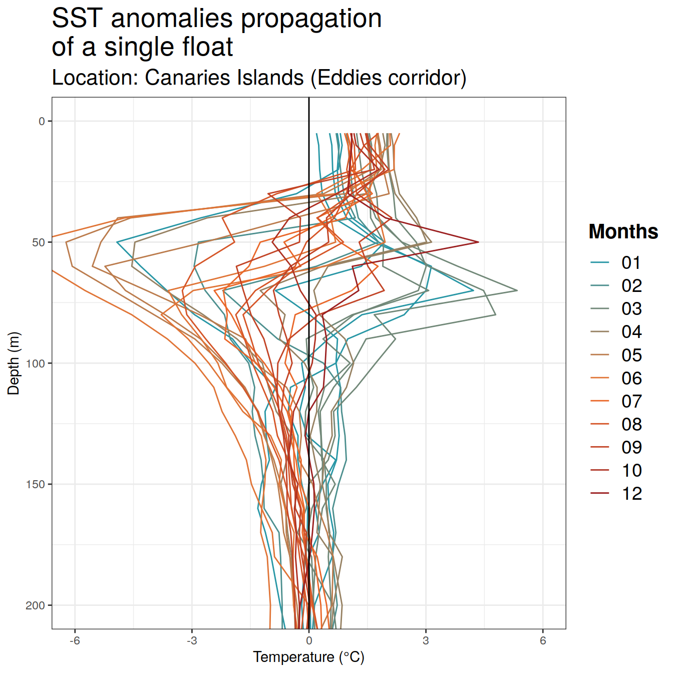
Individual float
Inspection of single floats to understand the physical processes impacting the argo floats measurements
unique_platform<-core_anomaly_2023_natlantic_subset %>%
  filter(platform_number==1902323)

ggplot() +
  geom_path(data=unique_platform, aes(x = anomaly, y = depth, color = factor(month), group = cycle_number)) +
  geom_vline(xintercept = 0) +
  scale_y_reverse() +
  coord_cartesian(xlim = c(-6, 6), ylim = c(200, 0)) +
    scale_color_manual(values = colorRampPalette(c("#2796A5", "#F3712B", "#880D1E"))(12)) +
    labs(title = 'SST anomalies propagation \nof a single float',
         subtitle = 'Location: Canaries Islands (Eddies corridor)',
       x = 'Temperature (°C)', y = 'Depth (m)', color = 'Months') +
   theme(plot.title = element_text(size = 20),
        plot.subtitle = element_text(size = 16),
        legend.text = element_text(size = 14),
        legend.title = element_text(size = 15, face = "bold")
        # legend.background = element_rect(fill = "transparent", color='transparent'),
        # legend.position=c(.91,.28),
    )
Coloring by lat/lon
Inspection of the potential spatial gradient that may influence the SST anomalies penetration: longitude and latitude gradients.
#Calculating monthly mean anomaly + std deviation for each lat/lon pair of the area
anomaly_lat_lon <- core_anomaly_2023_natlantic_subset %>%
  group_by(lat, lon, depth, month, platform_number, cycle_number) %>%
  summarise(
    temp_count = n(),
    temp_anomaly_mean = mean(anomaly, na.rm = TRUE)
    )

# Longitude - gradient north-south
longitude<- ggplot(anomaly_lat_lon, aes(x = temp_anomaly_mean, y = depth, group = interaction(platform_number, cycle_number), color = as.numeric(lon))) +
  geom_path() +
  geom_vline(xintercept = 0) +
  scale_y_reverse(limits = c(200, 0)) +
  coord_cartesian(xlim = c(-6, 6)) +
  facet_wrap(~ month, ncol = 3) +
  # labs(title = "Anomaly Profiles for all longitudes",
       # subtitle = "All floats and cycles included",
     labs(  x = "Temperature (°C)", y = "Depth (m)", color = "Longitude") +
  scale_color_viridis_c()+
  theme(plot.title = element_text(size = 20),
        plot.subtitle = element_text(size = 16),
        legend.text = element_text(size = 14),
        legend.title = element_text(size = 15, face = "bold"))

# Latitude - gradient west-east
latitude<- ggplot(anomaly_lat_lon, aes(x = temp_anomaly_mean, y = depth, group = interaction(platform_number, cycle_number), color = as.numeric(lat))) +
  geom_path() +
  geom_vline(xintercept = 0) +
  scale_y_reverse(limits = c(200, 0)) +
  coord_cartesian(xlim = c(-6, 6)) +
  facet_wrap(~ month, ncol = 3) +
  # labs(title = "Anomaly Profile for all latitudes",
       # subtitle = "All floats and cycles included",
       labs(x = "Temperature (°C)", y = "Depth (m)", color = "Latitude") +
  scale_color_viridis_c()+
  theme(plot.title = element_text(size = 20),
        plot.subtitle = element_text(size = 16),
        legend.text = element_text(size = 14),
        legend.title = element_text(size = 15, face = "bold"))


combined_plot <- latitude + longitude + plot_layout(ncol = 1)+
  plot_annotation(title = 'Latitude and longitude gradients',
                  subtitle = "All floats and cycles included",
                  theme = theme(plot.title = element_text(size = 18),
                                plot.subtitle = element_text(size = 16))
                  )
combined_plot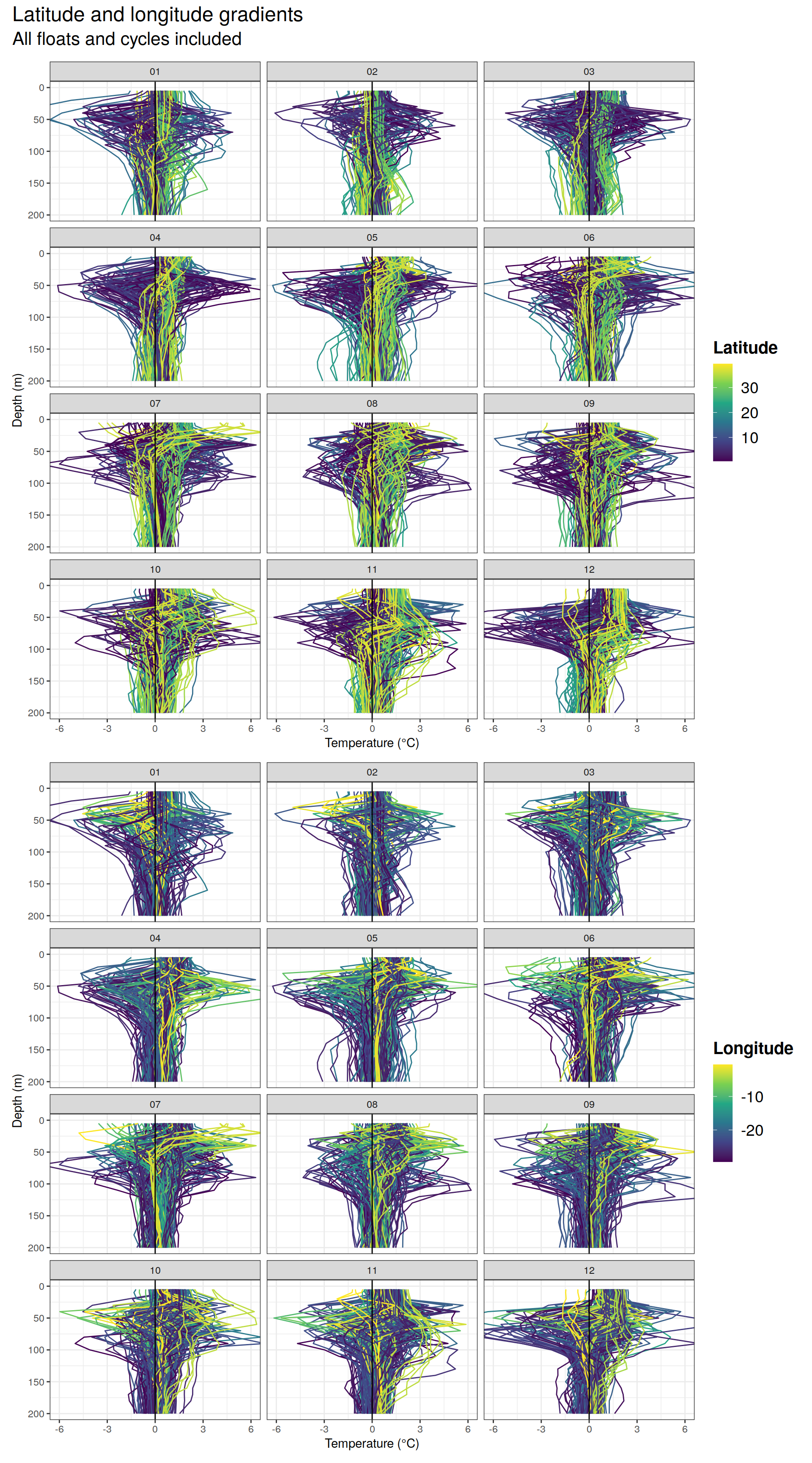
Coloring by SST anomaly
Looking at the SST anomalies that may influence the vertical structure of the MHS penetration
# calculate mean anomaly data
anomaly_summary <- core_anomaly_2023_natlantic_subset %>%
  group_by(platform_number, depth, month, cycle_number, SST_anomaly) %>%
  summarise(
    temp_count = n(),
    temp_anomaly_mean = mean(anomaly, na.rm = TRUE)
  )

#plot
ggplot(anomaly_summary, aes(x = temp_anomaly_mean, y = depth, group = interaction(platform_number, cycle_number), color = as.numeric(SST_anomaly))) +
  geom_path() +
  geom_vline(xintercept = 0) +
  scale_y_reverse(limits = c(200, 0)) +
  coord_cartesian(xlim = c(-6, 6)) +
    facet_wrap(~ month, ncol = 3) +
  labs(title = "Mean Anomaly Profile as a function of SST anomaly",
       x = "Temperature (°C)", y = "Depth (m)", color = "SST Anomaly") +
  scale_color_viridis_c()+
  theme(legend.key.width = unit(0.5, "cm"),
        legend.key.height = unit(2, "cm"))
Day within the month
# calculate mean anomaly data
anomaly_summary_day <- core_anomaly_2023_natlantic_subset %>%
  group_by(platform_number, depth, month, cycle_number, day) %>%
  summarise(
    temp_count = n(),
    temp_anomaly_mean = mean(anomaly, na.rm = TRUE)
  )
#plot for time during month
ggplot(anomaly_summary_day, aes(x = temp_anomaly_mean, y = depth, group = interaction(platform_number, cycle_number), color = as.numeric(day))) +
  geom_path() +
  geom_vline(xintercept = 0) +
  scale_y_reverse(limits = c(200, 0)) +
  coord_cartesian(xlim = c(-6, 6)) +
    facet_wrap(~ month, ncol = 3) +
  labs(title = "Mean Anomaly Profile as function of time",
       x = "Temperature (°C)", y = "Depth (m)", color = "day within \nthe month") +
  scale_color_viridis_c()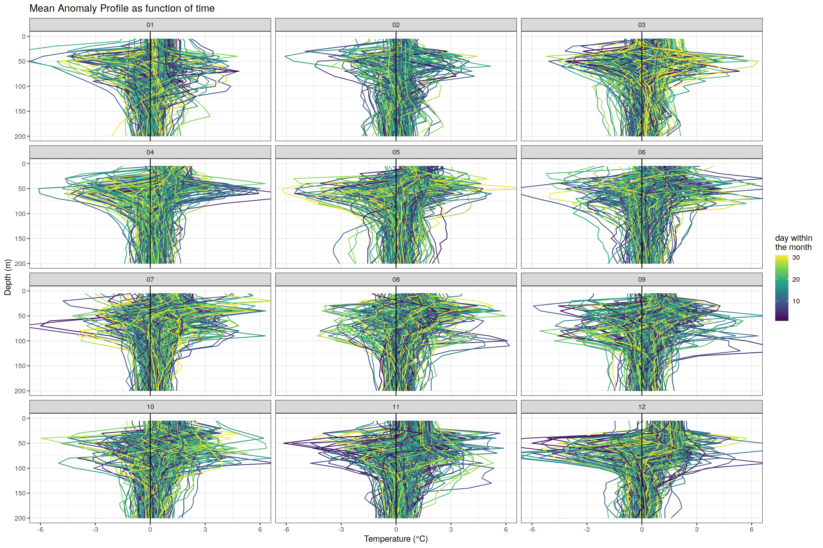
Monthly anomaly profiles
# Dataset with the cycle number per float across months
cycles_per_platform_month<- core_anomaly_2023_natlantic_subset %>%
  group_by(platform_number, month) %>%
  summarize(unique_cycles = toString(unique(cycle_number)))

# Calculating monthly mean anomaly + std dev over the east area by averaging the anomaly of each float present
anomaly_mean <- core_anomaly_2023_natlantic_subset %>%
  group_by(depth, month) %>%
  summarise(temp_count = n(),
            temp_anomaly_mean = mean(anomaly, na.rm = TRUE),
            temp_anomaly_sd = sd(anomaly, na.rm = TRUE))

#For each month: the SST anomaly and vertical anomaly profile plots next to each other
for (m in unique(core_anomaly_2023_natlantic_subset$month)) {
  # Filter data
  map_data <- filter(sst_anomaly_northAtlantic_subset, month == m)
  anomaly_data <- filter(anomaly_mean, month == m)

  # Plot for temperature anomaly map
  map_plot <- ggplot() +
    geom_tile(data=map_data, aes(x = lon, y = lat, fill = SST_anomaly)) +
    geom_map(data = world_coordinates, map = world_coordinates, aes(long, lat, map_id = region), fill = "grey") + #base map
    lims(x = c(chosen_extent$lon_min, chosen_extent$lon_max), y=c(chosen_extent$lat_min, chosen_extent$lat_max)) +
    coord_quickmap(expand = 0) +
    scale_fill_viridis_c(option = "magma") +
    labs(title = paste("SST Anomaly (°C) in North Atlantic - 2023", month.name[as.numeric(m)]),
         subtitle = paste0("Extent: ", name_extent),
         x = "Longitude", y = "Latitude") +
    theme(legend.position = 'right', legend.key.height = unit(2, "cm"),
          plot.title = element_text(size = 18),
          plot.subtitle = element_text(size = 16),
          legend.text = element_text(size = 13),
          legend.title = element_text(size = 15, face = "bold")
          # legend.background = element_rect(fill = "transparent", color='transparent'),
          # legend.position=c(.91,.28),
    )

  # Plot for anomaly profiles
  anomaly_plot <- ggplot(anomaly_data, aes(x = temp_anomaly_mean, y = depth, color = factor(month))) +
    geom_path() +
    geom_ribbon(aes(xmax = temp_anomaly_mean + temp_anomaly_sd,
                    xmin = temp_anomaly_mean - temp_anomaly_sd,
                    y = depth), alpha = 0.2) +
    geom_vline(xintercept = 0) +
    scale_y_reverse() +
    coord_cartesian(xlim = c(-4, 4), ylim = c(200, 0)) +
    labs(title = paste('Associated anomaly profile in', month.name[as.numeric(m)]),
         subtitle = paste0("from surface to 200m", "\nNumber of platform:",  nrow(filter(cycles_per_platform_month, month==m))),
         x = 'Temperature (°C)', y = 'Depth (m)') +
    theme_minimal()+
        guides(color = FALSE)+
    theme(legend.position = 'right', legend.key.height = unit(2, "cm"),
          plot.title = element_text(size = 18),
          plot.subtitle = element_text(size = 16),
          legend.text = element_text(size = 13),
          legend.title = element_text(size = 15, face = "bold")
        # legend.background = element_rect(fill = "transparent", color='transparent'),
        # legend.position=c(.91,.28),
    )


  #plots side by side
  combined_plot <- grid.arrange(map_plot, anomaly_plot, ncol = 2)
  print(combined_plot)
}
TableGrob (1 x 2) "arrange": 2 grobs
  z     cells    name           grob
1 1 (1-1,1-1) arrange gtable[layout]
2 2 (1-1,2-2) arrange gtable[layout]
TableGrob (1 x 2) "arrange": 2 grobs
  z     cells    name           grob
1 1 (1-1,1-1) arrange gtable[layout]
2 2 (1-1,2-2) arrange gtable[layout]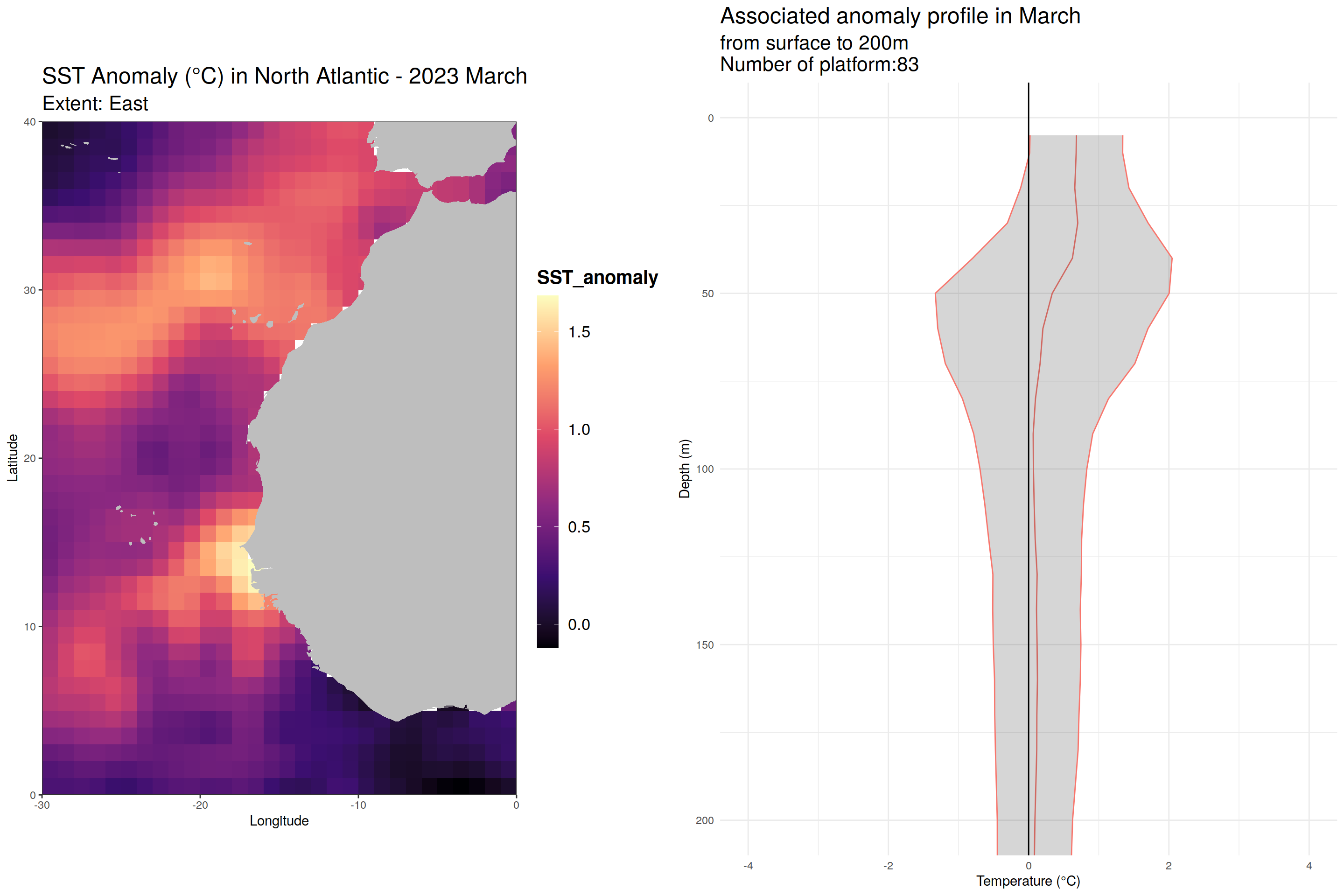
TableGrob (1 x 2) "arrange": 2 grobs
  z     cells    name           grob
1 1 (1-1,1-1) arrange gtable[layout]
2 2 (1-1,2-2) arrange gtable[layout]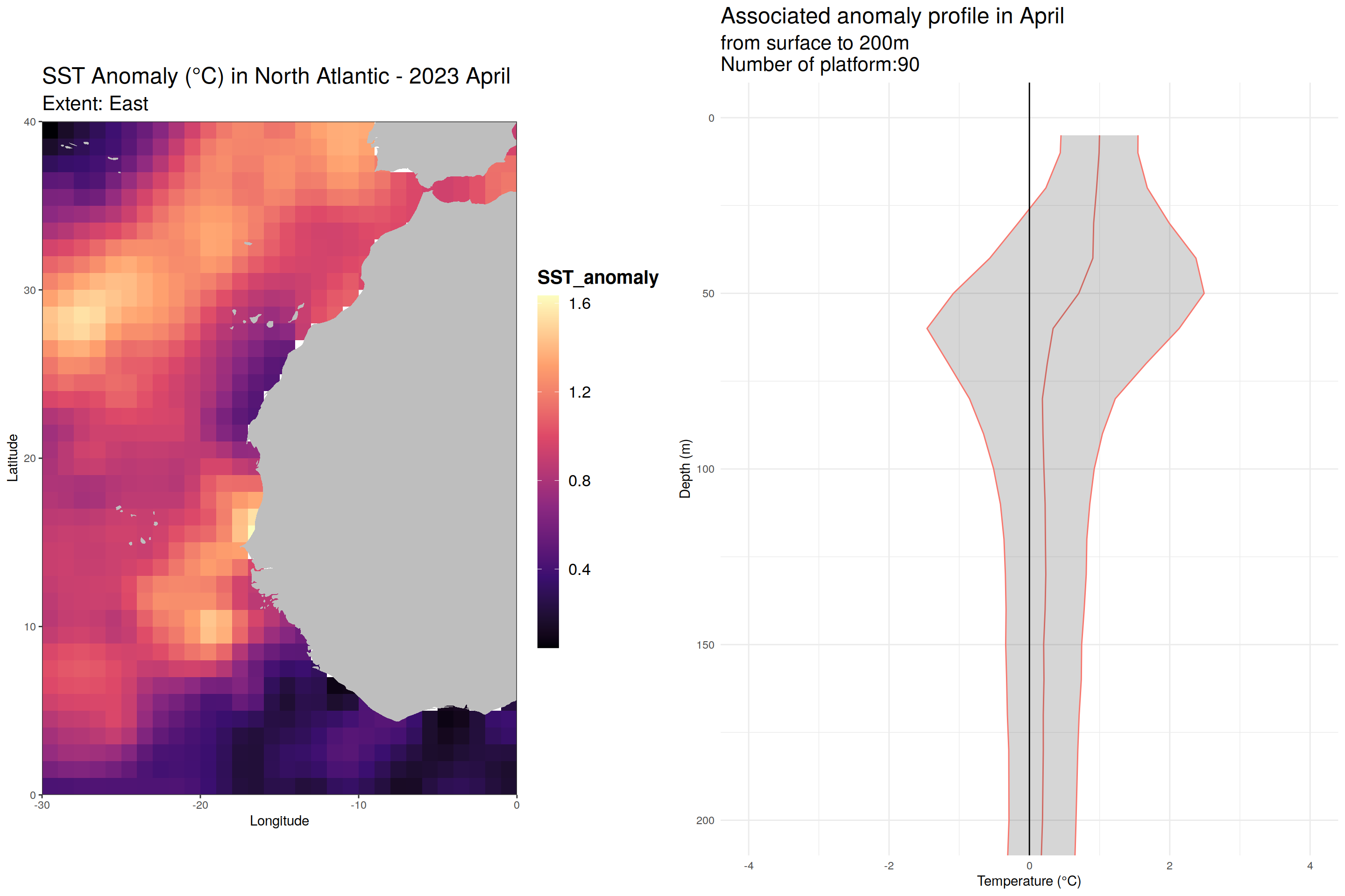
TableGrob (1 x 2) "arrange": 2 grobs
  z     cells    name           grob
1 1 (1-1,1-1) arrange gtable[layout]
2 2 (1-1,2-2) arrange gtable[layout]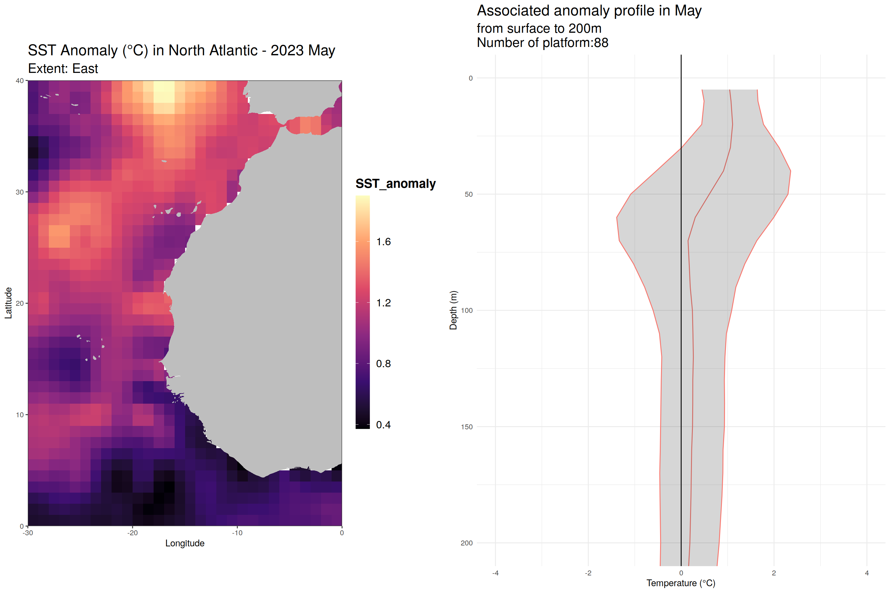
TableGrob (1 x 2) "arrange": 2 grobs
  z     cells    name           grob
1 1 (1-1,1-1) arrange gtable[layout]
2 2 (1-1,2-2) arrange gtable[layout]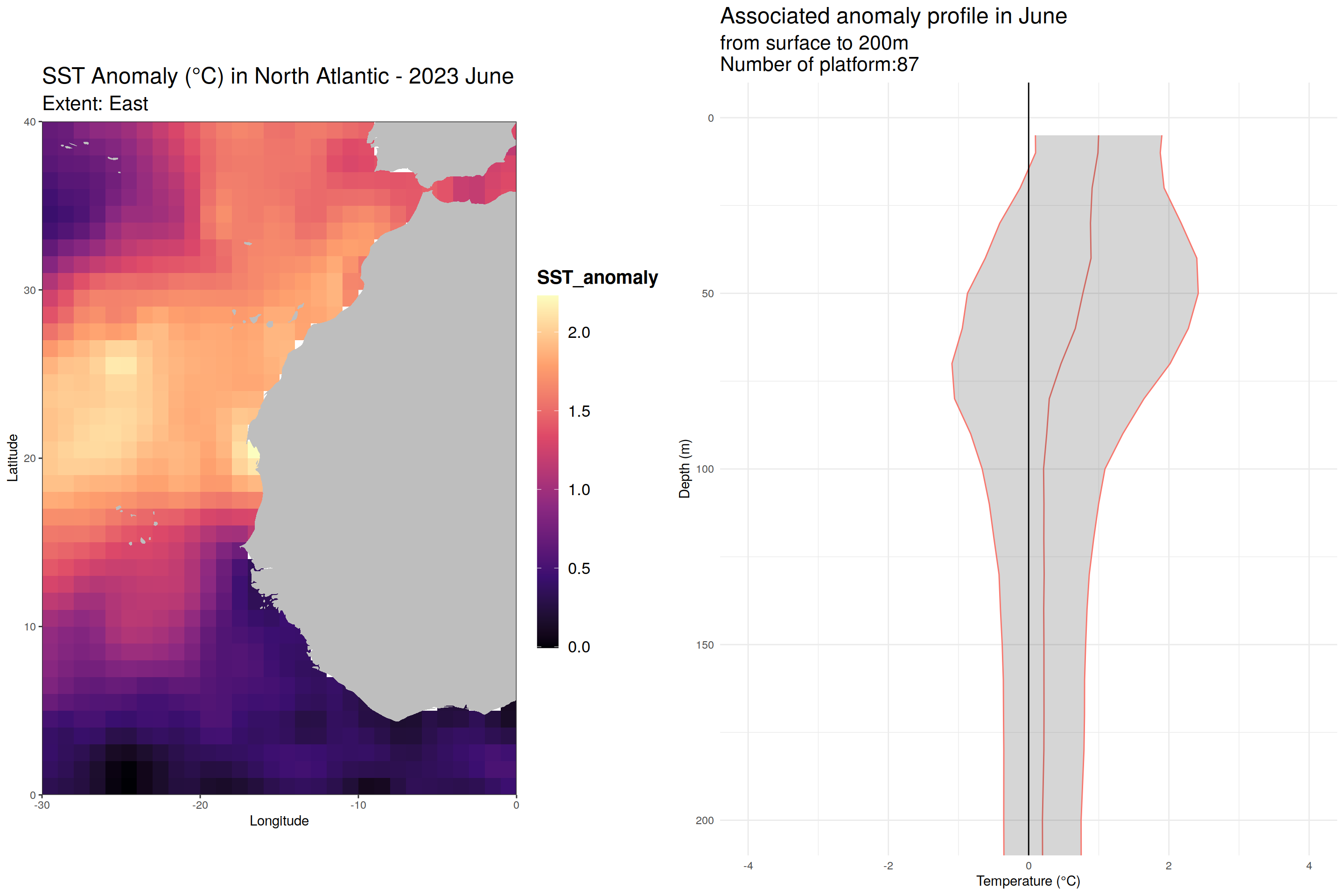
TableGrob (1 x 2) "arrange": 2 grobs
  z     cells    name           grob
1 1 (1-1,1-1) arrange gtable[layout]
2 2 (1-1,2-2) arrange gtable[layout]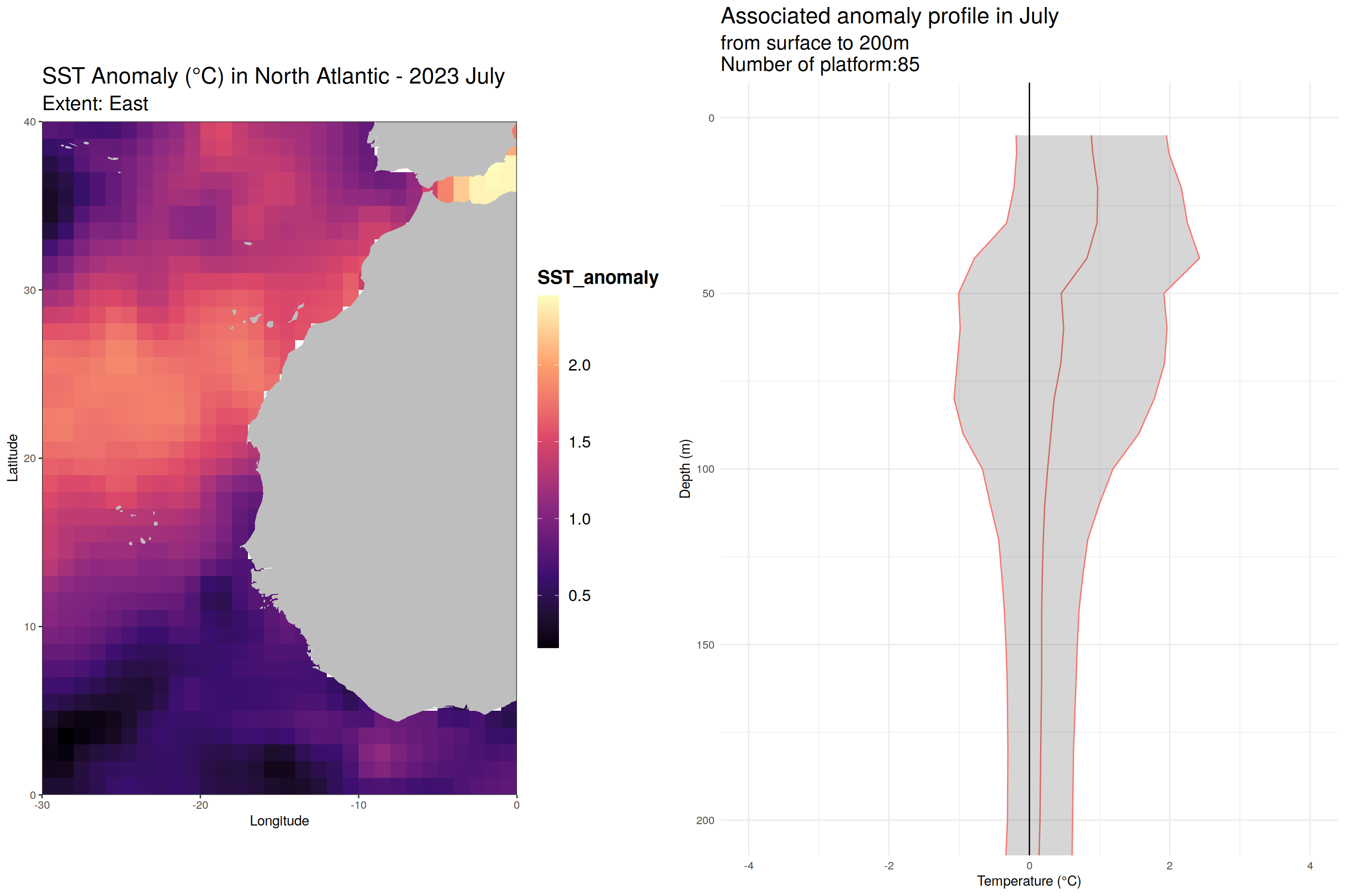
TableGrob (1 x 2) "arrange": 2 grobs
  z     cells    name           grob
1 1 (1-1,1-1) arrange gtable[layout]
2 2 (1-1,2-2) arrange gtable[layout]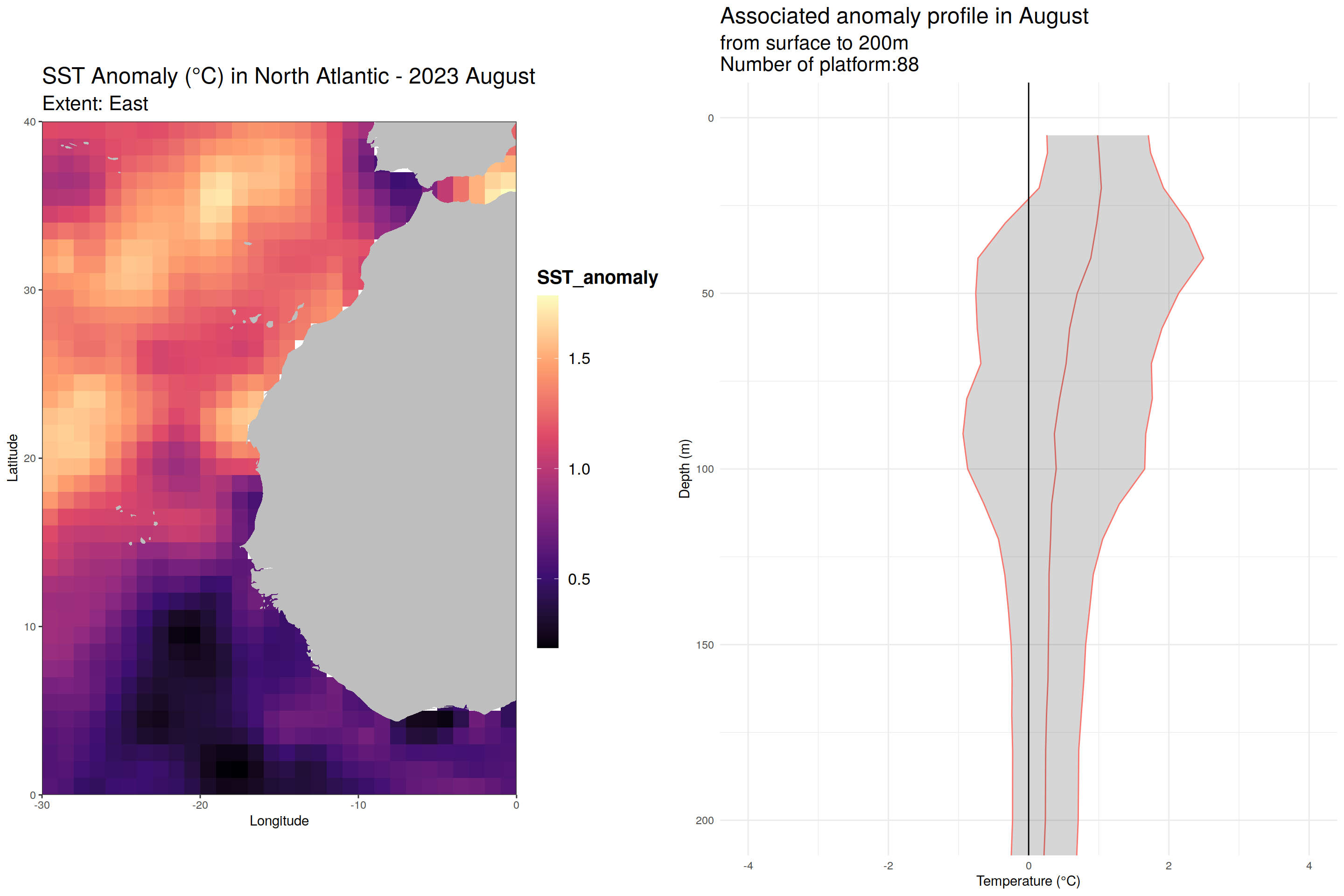
TableGrob (1 x 2) "arrange": 2 grobs
  z     cells    name           grob
1 1 (1-1,1-1) arrange gtable[layout]
2 2 (1-1,2-2) arrange gtable[layout]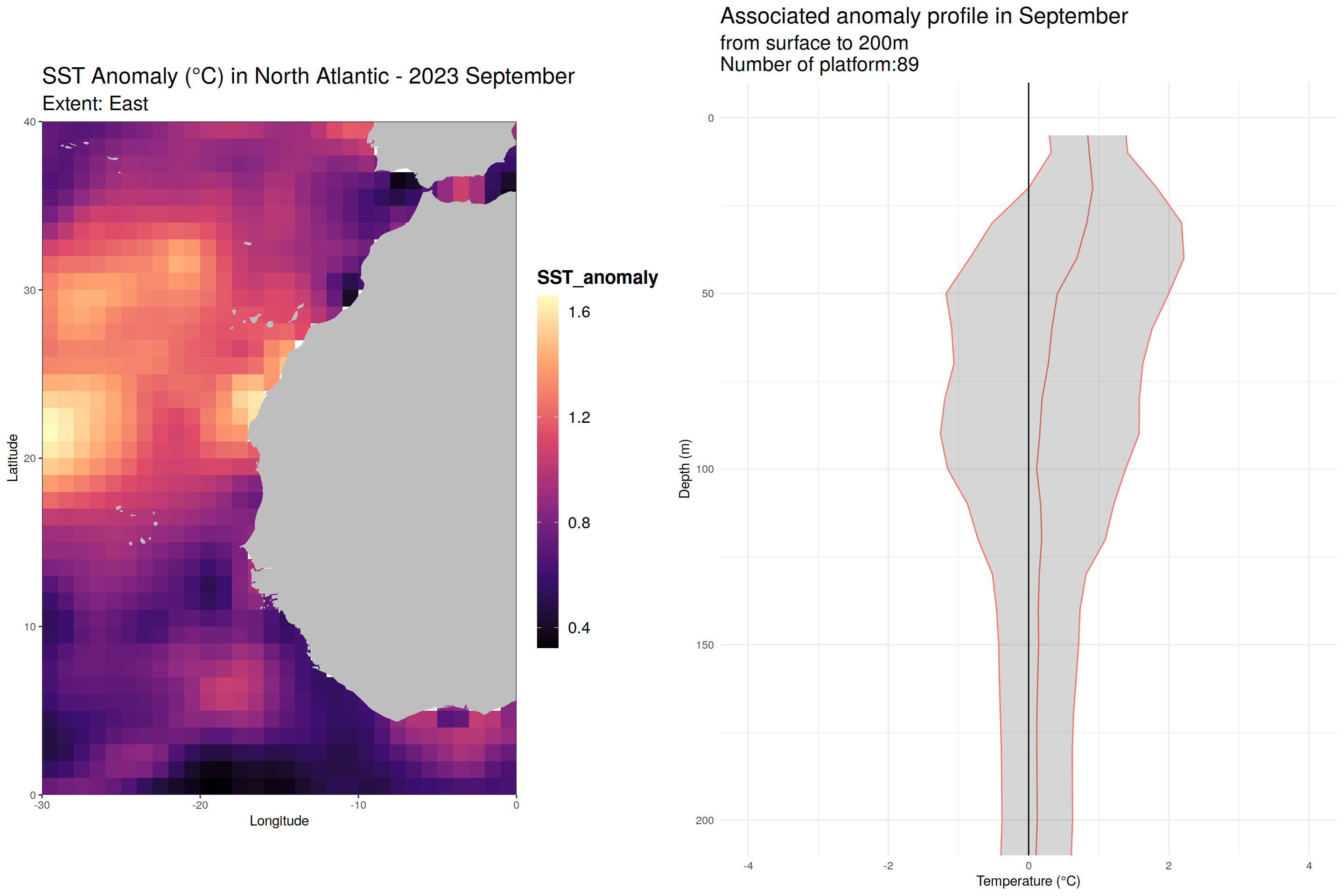
TableGrob (1 x 2) "arrange": 2 grobs
  z     cells    name           grob
1 1 (1-1,1-1) arrange gtable[layout]
2 2 (1-1,2-2) arrange gtable[layout]
TableGrob (1 x 2) "arrange": 2 grobs
  z     cells    name           grob
1 1 (1-1,1-1) arrange gtable[layout]
2 2 (1-1,2-2) arrange gtable[layout]
TableGrob (1 x 2) "arrange": 2 grobs
  z     cells    name           grob
1 1 (1-1,1-1) arrange gtable[layout]
2 2 (1-1,2-2) arrange gtable[layout]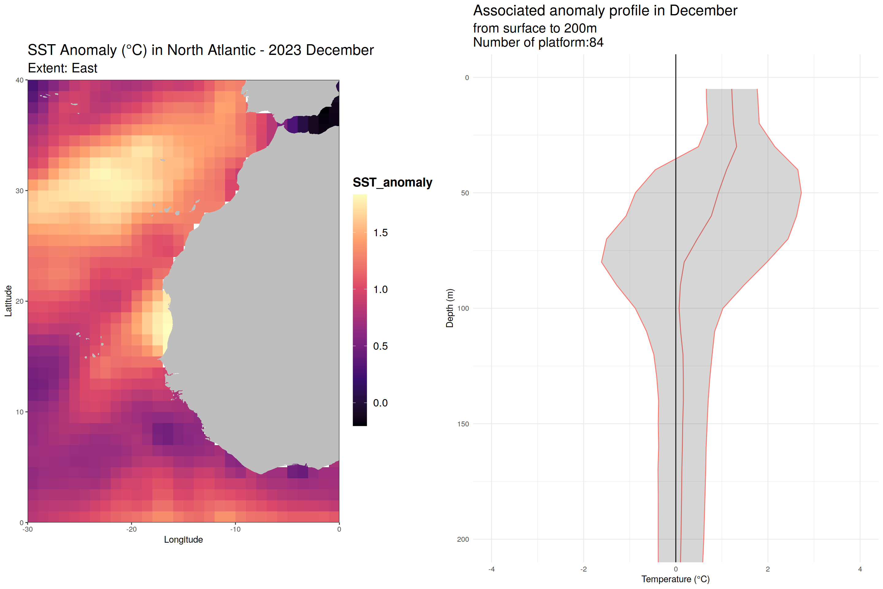
TableGrob (1 x 2) "arrange": 2 grobs
  z     cells    name           grob
1 1 (1-1,1-1) arrange gtable[layout]
2 2 (1-1,2-2) arrange gtable[layout]
# Vertical anomaly profile for the North Atlantic subset region - monthly
ggplot(anomaly_mean, aes(x = temp_anomaly_mean, y = depth, color = factor(month))) +
geom_path() +
geom_ribbon(aes(xmax = temp_anomaly_mean + temp_anomaly_sd,
xmin = temp_anomaly_mean - temp_anomaly_sd,
y = depth), alpha = 0.2) +
geom_vline(xintercept = 0) +
scale_y_reverse() +
coord_cartesian(xlim = c(-4, 4), ylim = c(200, 0)) +
labs(title = paste('Monthly anomaly profile'),
subtitle = paste0("Extent: ", name_extent),
x = 'Temperature (°C)', y = 'Depth (m)') +
guides(color = FALSE)+
facet_wrap(~month)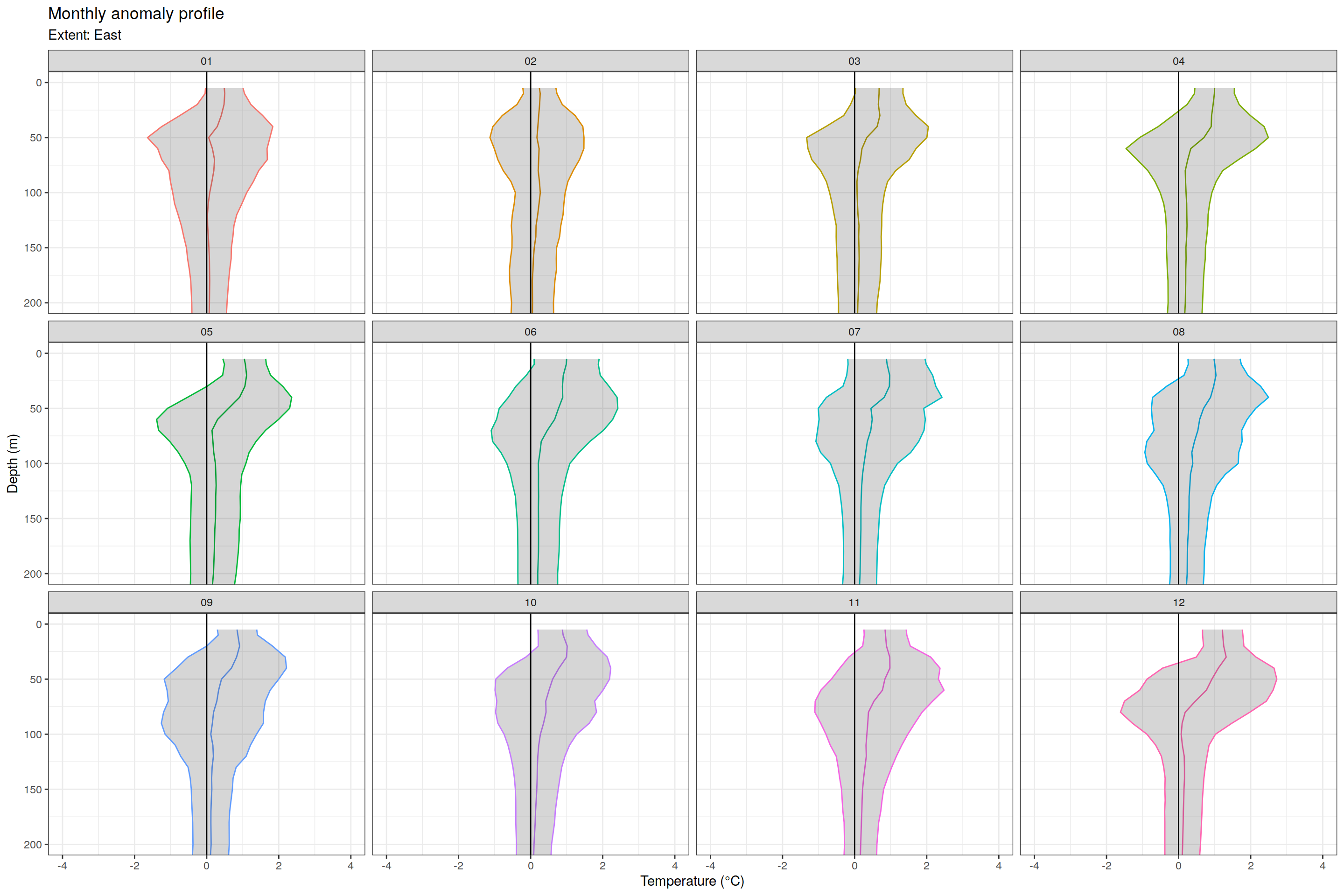
# Averaging the mean anomaly profiles on a 2 months period
anomaly_2months <- core_anomaly_2023_natlantic_subset %>%
  mutate(period=(as.numeric(month)+1)%/%2)

anomaly_2months<-anomaly_2months %>%
  group_by(depth, period) %>%
  summarise(temp_count = n(),
            temp_anomaly_mean = mean(anomaly, na.rm = TRUE),
            temp_anomaly_sd = sd(anomaly, na.rm = TRUE))

#Spread on the entire year
anomaly_2023<-core_anomaly_2023_natlantic_subset %>%
  group_by(depth) %>%
  summarise(temp_count = n(),
            temp_anomaly_mean = mean(anomaly, na.rm = TRUE),
            temp_anomaly_sd = sd(anomaly, na.rm = TRUE))

# Vertical anomaly profile for the North atlatinc east region - monthly
ggplot() +
  geom_path(data=anomaly_2months, aes(x = temp_anomaly_mean, y = depth, color = factor(period))) +
  geom_ribbon(data=anomaly_2023, aes(xmax = temp_anomaly_mean + temp_anomaly_sd, xmin = temp_anomaly_mean - temp_anomaly_sd, y = depth, fill = "spread"), alpha = 0.2) +
  geom_vline(xintercept = 0) +
  scale_y_reverse() +
  coord_cartesian(xlim = c(-4, 4), ylim = c(200, 0)) +
  labs(title = paste('Propagation of SST anomalies in the water column'),
       subtitle = paste0("Extent: ", name_extent, " North Atlantic bassin in ", target_year),
       x = 'Temperature (°C)', y = 'Depth (m)') +
  scale_color_manual(values =  colorRampPalette(c("blue", "orange", "darkred"))(6), # 2month mean anomalies color
                     breaks = unique(anomaly_2months$period),
                     labels =c("Jan-Feb", "March-April", "May-June", "July-Aug", "Sept-Oct", "Nov-Dec")) +
  scale_fill_manual(values = "grey", # Spread color
                    labels = "yearly") +
  theme(plot.title = element_text(size = 18),
        plot.subtitle = element_text(size = 12),
        legend.text = element_text(size = 14)) +
guides(color = guide_legend(title="Period"), fill = guide_legend(title = "Spread")) 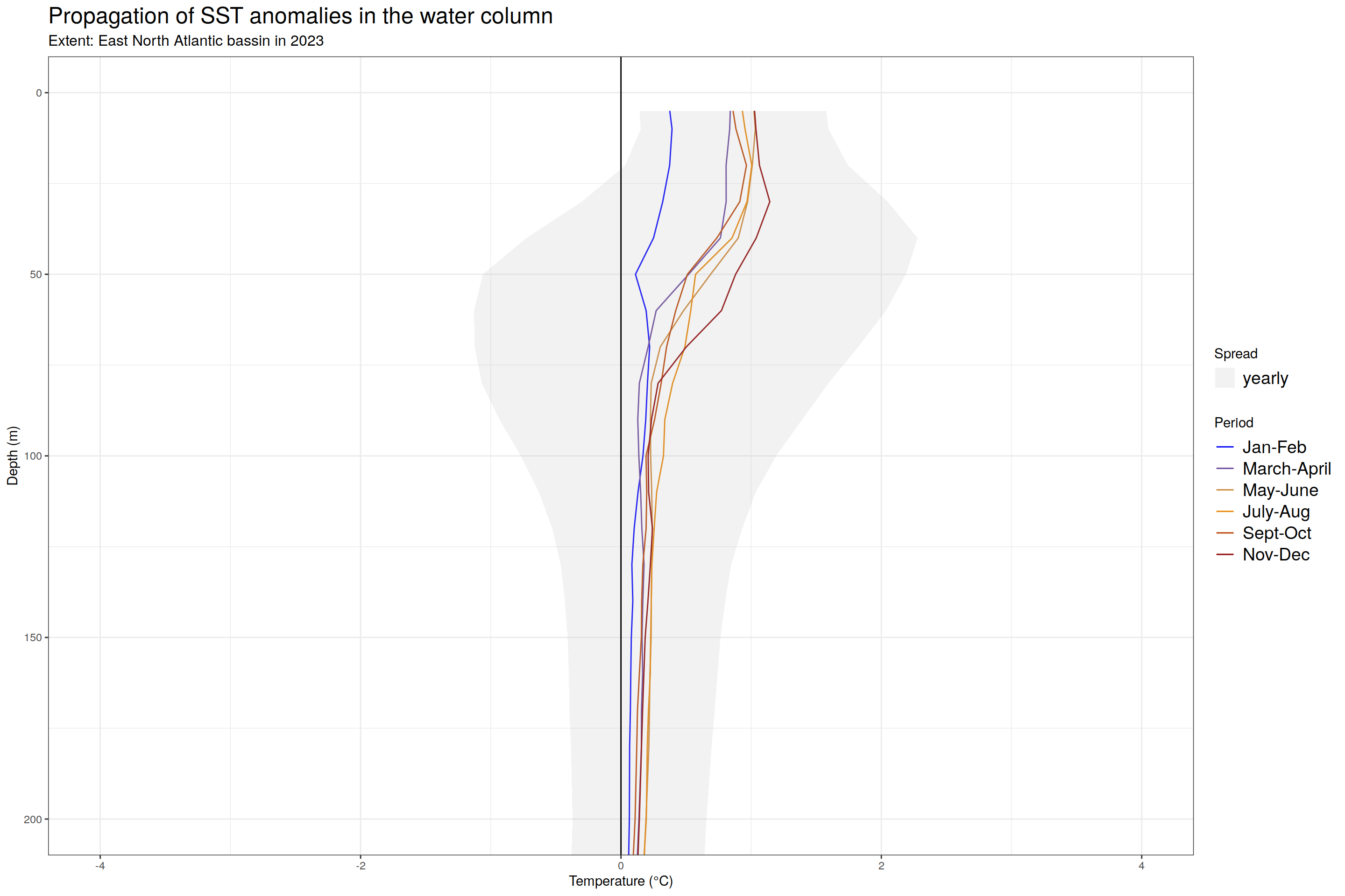
| Version | Author | Date |
|---|---|---|
| 3ac87c9 | mlarriere | 2024-05-20 |
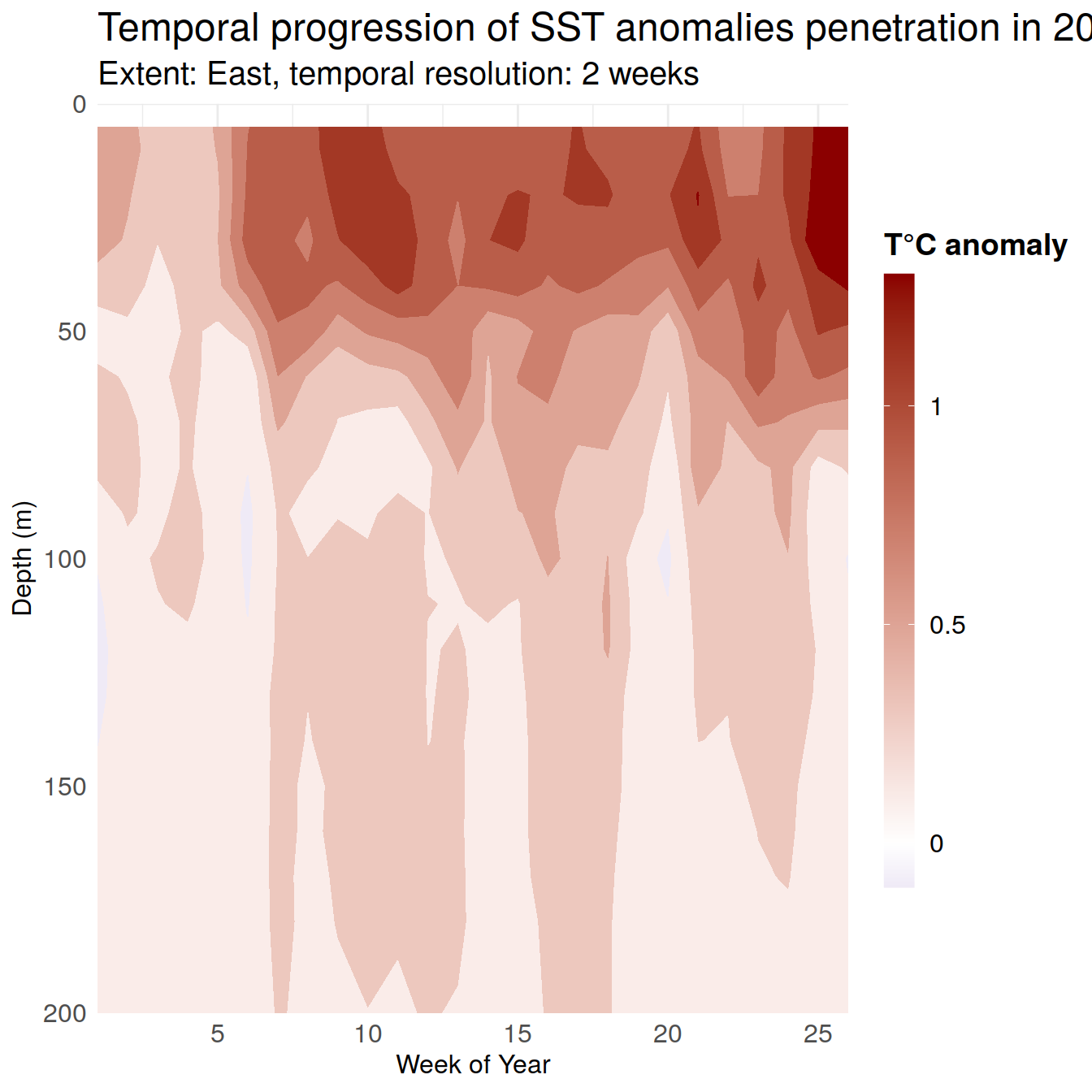
Hovmoeller plot
#---WEEKLY
#adding the week of the year
core_anomaly_2023_natlantic_subset <- core_anomaly_2023_natlantic_subset %>%
  mutate(week = week(date))

#---WEEKLY
anomaly_weekly<-core_anomaly_2023_natlantic_subset %>%
  group_by(depth, week) %>%
  summarise(temp_count = n(),
            temp_anomaly_mean = mean(anomaly, na.rm = TRUE))

#---2WEEKS
# Calculating monthly mean anomaly over the east area by averaging the anomaly of each float present
anomaly_2weekly <- core_anomaly_2023_natlantic_subset %>%
  mutate(week2=(week+1)%/%2) %>%
  group_by(depth, week2) %>%
  summarise(temp_count = n(),
            temp_anomaly_mean = mean(anomaly, na.rm = TRUE))

#---MONTHLY
anomaly_monthly <- core_anomaly_2023_natlantic_subset %>%
  group_by(depth, month) %>%
  summarise(temp_count = n(),
            temp_anomaly_mean = mean(anomaly, na.rm = TRUE))

#---Hovmoeller plot
breaks_seq=seq(-0.5,2, by=0.5)
labels_name=as.character(seq(-0.5,2, by=0.5))

ggplot(data=anomaly_2weekly, aes(x = week2, y = depth, z = temp_anomaly_mean)) +
  geom_contour_filled(aes(fill = after_stat(level_mid))) + #color = 'gray20', linewidth = 0.5,
  scale_fill_gradient2(name='T°C anomaly', low = "darkblue", high = "darkred", #low = "#CED3DC", high = "#906490"
                       breaks=seq(-0.5,2, by=0.5), labels=as.character(seq(-0.5,2, by=0.5))) +
  coord_cartesian(ylim = c(200, 0), expand = 0) +
  labs(title = "Temporal progression of SST anomalies penetration in 2023",
       subtitle = paste0("Extent: ", name_extent, ", temporal resolution: 2 weeks"),
       x = "Week of Year",       y = "Depth (m)") +
  theme_minimal() +
  theme(plot.title = element_text(size = 18),
        plot.subtitle = element_text(size = 15),
        axis.title.x = element_text(size = 12),
        axis.title.y = element_text(size = 12),
        axis.text.x = element_text(size = 12),
        axis.text.y = element_text(size = 12),
        legend.text = element_text(size = 12),
        # legend.position ='bottom' ,
        # legend.direction = "horizontal",  # Layout legend items horizontally
        # legend.box = "horizontal",
        legend.title = element_text(size = 14, face = "bold"),
        legend.key.width = unit(0.5, "cm"),
        legend.key.height = unit(2, "cm")
        )
| Version | Author | Date |
|---|---|---|
| 2d63792 | mlarriere | 2024-05-24 |
Mixed Layer Depth
Absolute maximum anomalies
#Absolute max anomalies for each lat-lon (1 value for each lat-lon pair)
abs_max_SSTanomalies<-core_anomaly_2023_natlantic_subset %>%
  filter(!is.na(anomaly), depth<=200) %>%
  group_by(lat, lon) %>%
  summarize(max_SST_anomaly = max(abs(anomaly), na.rm = TRUE))


plot1<-ggplot()+
  geom_tile(data=abs_max_SSTanomalies, aes(lon, lat, fill = max_SST_anomaly)) +
  geom_map(data = world_coordinates, map = world_coordinates, aes(long, lat, map_id = region), fill = "grey") +
  lims(x = c(chosen_extent$lon_min, chosen_extent$lon_max), y=c(chosen_extent$lat_min, chosen_extent$lat_max)) +
  scale_fill_viridis_c(option = "magma") +
  labs(title = "Absolute maximum SST anomaly",
       subtitle= "Annual average - 2023",
       fill = "Absolute max \nSST anomalies [°C]")+
  coord_quickmap(expand = 0)+
  theme(plot.title = element_text(size = 16),
        plot.subtitle = element_text(size = 12),
        legend.text = element_text(size = 10),
        legend.title = element_text(size = 11),
         legend.key.width = unit(0.5, "cm"),
        legend.key.height = unit(2, "cm")
        )


#Mean depth at which  max anomaly is found (maximum depth for each lat-lon pair)
mean_depth_max_anomaly<- inner_join(abs_max_SSTanomalies, core_anomaly_2023_natlantic_subset, by=c('lat', 'lon'))
mean_depth_max_anomaly <- mean_depth_max_anomaly %>%
  filter(abs(anomaly) == max_SST_anomaly)

plot2<-ggplot()+
  geom_tile(data=mean_depth_max_anomaly, aes(lon, lat, fill = depth)) +
  geom_map(data = world_coordinates, map = world_coordinates, aes(long, lat, map_id = region), fill = "grey") +
  lims(x = c(chosen_extent$lon_min, chosen_extent$lon_max), y=c(chosen_extent$lat_min, chosen_extent$lat_max)) +
  scale_fill_scico(palette = "lajolla", direction = -1) +

  # scale_fill_gradient2(name = 'Depth[m]', low = "darkblue", high = "darkred", midpoint = 100,
  #                      guide = "colorbar",
  #                      breaks=seq(0,1500, by=100), labels=as.character(seq(0,1500, by=100))) +
  labs(title = "Depth of maximum anomaly [m]",
       subtitle = 'depth range: 0-200m',
       fill = "Depth [m]")+
  coord_quickmap(expand = 0)+
   theme(plot.title = element_text(size = 16),
        plot.subtitle = element_text(size = 12),
        legend.text = element_text(size = 10),
        legend.title = element_text(size = 11),
         legend.key.width = unit(0.5, "cm"),
        legend.key.height = unit(2, "cm")
        )

combined_plot<-plot1+plot2
combined_plot
| Version | Author | Date |
|---|---|---|
| 2d63792 | mlarriere | 2024-05-24 |
sessionInfo()R version 4.2.2 (2022-10-31)
Platform: x86_64-pc-linux-gnu (64-bit)
Running under: openSUSE Leap 15.5
Matrix products: default
BLAS: /usr/local/R-4.2.2/lib64/R/lib/libRblas.so
LAPACK: /usr/local/R-4.2.2/lib64/R/lib/libRlapack.so
locale:
[1] LC_CTYPE=en_US.UTF-8 LC_NUMERIC=C
[3] LC_TIME=en_US.UTF-8 LC_COLLATE=en_US.UTF-8
[5] LC_MONETARY=en_US.UTF-8 LC_MESSAGES=en_US.UTF-8
[7] LC_PAPER=en_US.UTF-8 LC_NAME=C
[9] LC_ADDRESS=C LC_TELEPHONE=C
[11] LC_MEASUREMENT=en_US.UTF-8 LC_IDENTIFICATION=C
attached base packages:
[1] stats graphics grDevices utils datasets methods base
other attached packages:
[1] scico_1.3.1 patchwork_1.1.2 broom_1.0.5
[4] paletteer_1.6.0 cluster_2.1.6 gridExtra_2.3
[7] scatterplot3d_0.3-44 viridis_0.6.2 viridisLite_0.4.1
[10] ggOceanMaps_1.3.4 ggspatial_1.1.7 oce_1.7-10
[13] gsw_1.1-1 lubridate_1.9.0 timechange_0.1.1
[16] forcats_0.5.2 stringr_1.5.0 dplyr_1.1.3
[19] purrr_1.0.2 readr_2.1.3 tidyr_1.3.0
[22] tibble_3.2.1 ggplot2_3.4.4 tidyverse_1.3.2
[25] workflowr_1.7.0
loaded via a namespace (and not attached):
[1] googledrive_2.0.0 colorspace_2.0-3 ellipsis_0.3.2
[4] class_7.3-20 rprojroot_2.0.3 fs_1.5.2
[7] rstudioapi_0.15.0 proxy_0.4-27 farver_2.1.1
[10] fansi_1.0.3 xml2_1.3.3 codetools_0.2-18
[13] cachem_1.0.6 knitr_1.41 jsonlite_1.8.3
[16] dbplyr_2.2.1 rgeos_0.5-9 compiler_4.2.2
[19] httr_1.4.4 backports_1.4.1 assertthat_0.2.1
[22] fastmap_1.1.0 gargle_1.2.1 cli_3.6.1
[25] later_1.3.0 htmltools_0.5.8.1 tools_4.2.2
[28] gtable_0.3.1 glue_1.6.2 maps_3.4.1
[31] Rcpp_1.0.10 cellranger_1.1.0 jquerylib_0.1.4
[34] RNetCDF_2.6-1 raster_3.6-11 vctrs_0.6.4
[37] lwgeom_0.2-10 xfun_0.35 ps_1.7.2
[40] rvest_1.0.3 lifecycle_1.0.3 ncmeta_0.3.5
[43] googlesheets4_1.0.1 terra_1.7-65 getPass_0.2-2
[46] scales_1.2.1 hms_1.1.2 promises_1.2.0.1
[49] parallel_4.2.2 rematch2_2.1.2 yaml_2.3.6
[52] sass_0.4.4 stringi_1.7.8 highr_0.9
[55] e1071_1.7-12 rlang_1.1.1 pkgconfig_2.0.3
[58] evaluate_0.18 lattice_0.20-45 sf_1.0-9
[61] labeling_0.4.2 processx_3.8.0 tidyselect_1.2.0
[64] magrittr_2.0.3 R6_2.5.1 generics_0.1.3
[67] DBI_1.2.2 pillar_1.9.0 haven_2.5.1
[70] whisker_0.4 withr_2.5.0 units_0.8-0
[73] stars_0.6-0 abind_1.4-5 sp_1.5-1
[76] modelr_0.1.10 crayon_1.5.2 KernSmooth_2.23-20
[79] utf8_1.2.2 tzdb_0.3.0 rmarkdown_2.18
[82] isoband_0.2.6 grid_4.2.2 readxl_1.4.1
[85] callr_3.7.3 git2r_0.30.1 reprex_2.0.2
[88] digest_0.6.30 classInt_0.4-8 httpuv_1.6.6
[91] munsell_0.5.0 bslib_0.4.1