Budgets

workflowr

• Summary
• Checks
• Past versions

Last updated: 2022-11-11

Checks: 7 0

Knit directory: emlr_obs_analysis/analysis/

This reproducible R Markdown analysis was created with workflowr (version 1.7.0). The Checks tab describes the reproducibility checks that were applied when the results were created. The Past versions tab lists the development history.

---

R Markdown file: up-to-date

Great! Since the R Markdown file has been committed to the Git repository, you know the exact version of the code that produced these results.

Environment: empty

Great job! The global environment was empty. Objects defined in the global environment can affect the analysis in your R Markdown file in unknown ways. For reproduciblity it’s best to always run the code in an empty environment.

Seed: set.seed(20210412)

The command set.seed(20210412) was run prior to running the code in the R Markdown file. Setting a seed ensures that any results that rely on randomness, e.g. subsampling or permutations, are reproducible.

Session information: recorded

Great job! Recording the operating system, R version, and package versions is critical for reproducibility.

Cache: none

Nice! There were no cached chunks for this analysis, so you can be confident that you successfully produced the results during this run.

File paths: relative

Great job! Using relative paths to the files within your workflowr project makes it easier to run your code on other machines.

Repository version: c53fea0

Great! You are using Git for version control. Tracking code development and connecting the code version to the results is critical for reproducibility.

The results in this page were generated with repository version c53fea0. See the Past versions tab to see a history of the changes made to the R Markdown and HTML files.

Note that you need to be careful to ensure that all relevant files for the analysis have been committed to Git prior to generating the results (you can use wflow_publish or wflow_git_commit). workflowr only checks the R Markdown file, but you know if there are other scripts or data files that it depends on. Below is the status of the Git repository when the results were generated:

Ignored files:
    Ignored:    .Rhistory
    Ignored:    .Rproj.user/
    Ignored:    data/
    Ignored:    output/other/
    Ignored:    output/presentation/
    Ignored:    output/publication/

Unstaged changes:
    Modified:   analysis/_site.yml
    Modified:   code/Workflowr_project_managment.R

Note that any generated files, e.g. HTML, png, CSS, etc., are not included in this status report because it is ok for generated content to have uncommitted changes.

---

These are the previous versions of the repository in which changes were made to the R Markdown (analysis/WOA18_budgets.Rmd) and HTML (docs/WOA18_budgets.html) files. If you’ve configured a remote Git repository (see ?wflow_git_remote), click on the hyperlinks in the table below to view the files as they were in that past version.

File	Version	Author	Date	Message
Rmd	c53fea0	jens-daniel-mueller	2022-11-11	rebuild website with woa18 clim

---

version_id_pattern <- "n"
config <- "MLR_basins"

1 Read files

print(version_id_pattern)

[1] "n"

# identify required version IDs

Version_IDs_1 <- list.files(path = "/nfs/kryo/work/jenmueller/emlr_cant/observations",
                            pattern = paste0("v_1", "n"))

Version_IDs_2 <- list.files(path = "/nfs/kryo/work/jenmueller/emlr_cant/observations",
                            pattern = paste0("v_2", "n"))

Version_IDs_3 <- list.files(path = "/nfs/kryo/work/jenmueller/emlr_cant/observations",
                            pattern = paste0("v_3", "n"))

Version_IDs <- c(Version_IDs_1, Version_IDs_2, Version_IDs_3)

# print(Version_IDs)

1.1 Global

for (i_Version_IDs in Version_IDs) {
  # i_Version_IDs <- Version_IDs[1]
  
  # print(i_Version_IDs)
  
  path_version_data     <-
    paste(path_observations,
          i_Version_IDs,
          "/data/",
          sep = "")
  
  # load and join data files
  
  dcant_budget_global <-
    read_csv(paste(path_version_data,
                   "dcant_budget_global.csv",
                   sep = ""))
  
  dcant_budget_global_mod_truth <-
    read_csv(paste(
      path_version_data,
      "dcant_budget_global_mod_truth.csv",
      sep = ""
    ))
  
  dcant_budget_global_bias <-
    read_csv(paste(path_version_data,
                   "dcant_budget_global_bias.csv",
                   sep = ""))
  
  lm_best_predictor_counts <-
    read_csv(paste(path_version_data,
                   "lm_best_predictor_counts.csv",
                   sep = ""))
  
  lm_best_dcant <-
    read_csv(paste(path_version_data,
                   "lm_best_dcant.csv",
                   sep = ""))
  
  dcant_budget_global <- bind_rows(dcant_budget_global,
                                      dcant_budget_global_mod_truth)
  
  dcant_budget_global <- dcant_budget_global %>%
    mutate(Version_ID = i_Version_IDs)
  
  dcant_budget_global_bias <- dcant_budget_global_bias %>%
    mutate(Version_ID = i_Version_IDs)
  
  lm_best_predictor_counts <- lm_best_predictor_counts %>%
    mutate(Version_ID = i_Version_IDs)
  
  lm_best_dcant <- lm_best_dcant %>%
    mutate(Version_ID = i_Version_IDs)

  params_local <-
    read_rds(paste(path_version_data,
                   "params_local.rds",
                   sep = ""))
  
  params_local <- bind_cols(
    Version_ID = i_Version_IDs,
    MLR_basins := str_c(params_local$MLR_basins, collapse = "|"),
    tref1 = params_local$tref1,
    tref2 = params_local$tref2)
  
  tref <- read_csv(paste(path_version_data,
                         "tref.csv",
                         sep = ""))
  
  params_local <- params_local %>%
    mutate(
      median_year_1 = sort(tref$median_year)[1],
      median_year_2 = sort(tref$median_year)[2],
      duration = median_year_2 - median_year_1,
      period = paste(median_year_1, "-", median_year_2)
    )
  
  if (exists("dcant_budget_global_all")) {
    dcant_budget_global_all <-
      bind_rows(dcant_budget_global_all, dcant_budget_global)
  }
  
  if (!exists("dcant_budget_global_all")) {
    dcant_budget_global_all <- dcant_budget_global
  }
  
  if (exists("dcant_budget_global_bias_all")) {
    dcant_budget_global_bias_all <-
      bind_rows(dcant_budget_global_bias_all,
                dcant_budget_global_bias)
  }

  if (!exists("dcant_budget_global_bias_all")) {
    dcant_budget_global_bias_all <- dcant_budget_global_bias
  }
  
    
  if (exists("lm_best_predictor_counts_all")) {
    lm_best_predictor_counts_all <-
      bind_rows(lm_best_predictor_counts_all, lm_best_predictor_counts)
  }
  
  if (!exists("lm_best_predictor_counts_all")) {
    lm_best_predictor_counts_all <- lm_best_predictor_counts
  }
    
  if (exists("lm_best_dcant_all")) {
    lm_best_dcant_all <-
      bind_rows(lm_best_dcant_all, lm_best_dcant)
  }
  
  if (!exists("lm_best_dcant_all")) {
    lm_best_dcant_all <- lm_best_dcant
  }
  
  if (exists("params_local_all")) {
    params_local_all <- bind_rows(params_local_all, params_local)
  }
  
  if (!exists("params_local_all")) {
    params_local_all <- params_local
  }
  
  
}

rm(
  dcant_budget_global,
  dcant_budget_global_bias,
  dcant_budget_global_mod_truth,
  lm_best_predictor_counts,
  lm_best_dcant,
  params_local,
  tref
)

1.2 Basins

# Version_IDs <- Version_IDs[1:length(Version_IDs)-1]

for (i_Version_IDs in Version_IDs) {
  # i_Version_IDs <- Version_IDs[1]
  
  # print(i_Version_IDs)
  
  path_version_data     <-
    paste(path_observations,
          i_Version_IDs,
          "/data/",
          sep = "")
  
  # load and join data files
  
  dcant_budget_basin_AIP <-
    read_csv(paste(path_version_data,
                   "dcant_budget_basin_AIP.csv",
                   sep = ""))
  
  dcant_budget_basin_AIP_mod_truth <-
    read_csv(paste(
      path_version_data,
      "dcant_budget_basin_AIP_mod_truth.csv",
      sep = ""
    ))
  
    
  dcant_budget_basin_AIP <- bind_rows(dcant_budget_basin_AIP,
                                      dcant_budget_basin_AIP_mod_truth)
  
  dcant_budget_basin_AIP_bias <-
    read_csv(paste(path_version_data,
                   "dcant_budget_basin_AIP_bias.csv",
                   sep = ""))
  
  dcant_slab_budget_bias <-
    read_csv(paste0(path_version_data,
                    "dcant_slab_budget_bias.csv"))

  dcant_slab_budget <-
    read_csv(paste0(path_version_data,
                    "dcant_slab_budget.csv"))

  dcant_budget_basin_AIP <- dcant_budget_basin_AIP %>%
    mutate(Version_ID = i_Version_IDs)
  
  dcant_budget_basin_AIP_bias <- dcant_budget_basin_AIP_bias %>%
    mutate(Version_ID = i_Version_IDs)
  
  dcant_slab_budget <- dcant_slab_budget %>%
    mutate(Version_ID = i_Version_IDs)
  
  dcant_slab_budget_bias <- dcant_slab_budget_bias %>%
    mutate(Version_ID = i_Version_IDs)
  
  if (exists("dcant_budget_basin_AIP_all")) {
    dcant_budget_basin_AIP_all <-
      bind_rows(dcant_budget_basin_AIP_all, dcant_budget_basin_AIP)
  }
  
  if (!exists("dcant_budget_basin_AIP_all")) {
    dcant_budget_basin_AIP_all <- dcant_budget_basin_AIP
  }
  
  if (exists("dcant_budget_basin_AIP_bias_all")) {
    dcant_budget_basin_AIP_bias_all <-
      bind_rows(dcant_budget_basin_AIP_bias_all,
                dcant_budget_basin_AIP_bias)
  }
  
  if (!exists("dcant_budget_basin_AIP_bias_all")) {
    dcant_budget_basin_AIP_bias_all <- dcant_budget_basin_AIP_bias
  }
  
  if (exists("dcant_slab_budget_all")) {
    dcant_slab_budget_all <-
      bind_rows(dcant_slab_budget_all, dcant_slab_budget)
  }
  
  if (!exists("dcant_slab_budget_all")) {
    dcant_slab_budget_all <- dcant_slab_budget
  }
  
  if (exists("dcant_slab_budget_bias_all")) {
    dcant_slab_budget_bias_all <-
      bind_rows(dcant_slab_budget_bias_all,
                dcant_slab_budget_bias)
  }
  
  if (!exists("dcant_slab_budget_bias_all")) {
    dcant_slab_budget_bias_all <- dcant_slab_budget_bias
  }
  
}

rm(
  dcant_budget_basin_AIP,
  dcant_budget_basin_AIP_bias,
  dcant_budget_basin_AIP_mod_truth,
  dcant_slab_budget,
  dcant_slab_budget_bias
)

1.3 Basins hemisphere

# Version_IDs <- Version_IDs[1:length(Version_IDs)-1]

for (i_Version_IDs in Version_IDs) {
  # i_Version_IDs <- Version_IDs[1]
  
  # print(i_Version_IDs)
  
  path_version_data     <-
    paste(path_observations,
          i_Version_IDs,
          "/data/",
          sep = "")
  
  # load and join data files
  
  dcant_budget_basin_MLR <-
    read_csv(paste(path_version_data,
                   "dcant_budget_basin_MLR.csv",
                   sep = ""))
  
  dcant_budget_basin_MLR_mod_truth <-
    read_csv(paste(
      path_version_data,
      "dcant_budget_basin_MLR_mod_truth.csv",
      sep = ""
    ))
  
    
  dcant_budget_basin_MLR <- bind_rows(dcant_budget_basin_MLR,
                                      dcant_budget_basin_MLR_mod_truth)
  

  dcant_budget_basin_MLR <- dcant_budget_basin_MLR %>%
    mutate(Version_ID = i_Version_IDs)

  if (exists("dcant_budget_basin_MLR_all")) {
    dcant_budget_basin_MLR_all <-
      bind_rows(dcant_budget_basin_MLR_all, dcant_budget_basin_MLR)
  }
  
  if (!exists("dcant_budget_basin_MLR_all")) {
    dcant_budget_basin_MLR_all <- dcant_budget_basin_MLR
  }

  
}

rm(
  dcant_budget_basin_MLR,
  dcant_budget_basin_MLR_mod_truth
)

1.4 Steady state

for (i_Version_IDs in Version_IDs) {
  # i_Version_IDs <- Version_IDs[1]
  
  # print(i_Version_IDs)
  
  path_version_data     <-
    paste(path_observations,
          i_Version_IDs,
          "/data/",
          sep = "")
  
  # load and join data files
  
  dcant_obs_budget <-
    read_csv(paste0(path_version_data,
                    "anom_dcant_obs_budget.csv"))
  
  dcant_obs_budget <- dcant_obs_budget %>%
    mutate(Version_ID = i_Version_IDs)
  
  if (exists("dcant_obs_budget_all")) {
    dcant_obs_budget_all <-
      bind_rows(dcant_obs_budget_all, dcant_obs_budget)
  }
  
  if (!exists("dcant_obs_budget_all")) {
    dcant_obs_budget_all <- dcant_obs_budget
  }
  
}


rm(dcant_obs_budget)

1.5 Atm CO2

co2_atm <-
  read_csv(paste(path_preprocessing,
                 "co2_atm.csv",
                 sep = ""))

all_predictors <- c("saltempaouoxygenphosphatenitratesilicate")

params_local_all <- params_local_all %>%
  mutate(MLR_predictors = str_remove_all(all_predictors,
                                         MLR_predictors))

dcant_budget_global_all <- dcant_budget_global_all %>%
  filter(estimate == "dcant", 
         method == "total") %>% 
  select(-c(estimate, method)) %>% 
  rename(dcant = value)

dcant_budget_global_all_depth <- dcant_budget_global_all

dcant_budget_global_all <- dcant_budget_global_all %>%
  filter(inv_depth == params_global$inventory_depth_standard)

dcant_budget_global_bias_all <- dcant_budget_global_bias_all %>%
  filter(estimate == "dcant") %>%
  select(-c(estimate))

dcant_budget_global_bias_all_depth <- dcant_budget_global_bias_all

dcant_budget_global_bias_all <- dcant_budget_global_bias_all %>%
  filter(inv_depth == params_global$inventory_depth_standard)

dcant_budget_basin_AIP_all <- dcant_budget_basin_AIP_all %>%
  filter(estimate == "dcant", 
         method == "total") %>% 
  select(-c(estimate, method)) %>% 
  rename(dcant = value)

dcant_budget_basin_AIP_all_depth <- dcant_budget_basin_AIP_all

dcant_budget_basin_AIP_all <- dcant_budget_basin_AIP_all %>%
  filter(inv_depth == params_global$inventory_depth_standard)

dcant_budget_basin_AIP_bias_all <- dcant_budget_basin_AIP_bias_all %>%
  filter(estimate == "dcant") %>% 
  select(-c(estimate))

dcant_budget_basin_AIP_bias_all_depth <- dcant_budget_basin_AIP_bias_all

dcant_budget_basin_AIP_bias_all <- dcant_budget_basin_AIP_bias_all %>%
  filter(inv_depth == params_global$inventory_depth_standard)

dcant_budget_basin_MLR_all <- dcant_budget_basin_MLR_all %>%
  filter(estimate == "dcant", 
         method == "total") %>% 
  select(-c(estimate, method)) %>% 
  rename(dcant = value)

# dcant_budget_basin_MLR_all_depth <- dcant_budget_basin_MLR_all

dcant_budget_basin_MLR_all <- dcant_budget_basin_MLR_all %>%
  filter(inv_depth == params_global$inventory_depth_standard)

# dcant_budget_basin_MLR_bias_all <- dcant_budget_basin_MLR_bias_all %>%
#   filter(estimate == "dcant") %>% 
#   select(-c(estimate))
# 
# dcant_budget_basin_MLR_bias_all_depth <- dcant_budget_basin_MLR_bias_all
# 
# dcant_budget_basin_MLR_bias_all <- dcant_budget_basin_MLR_bias_all %>%
#   filter(inv_depth == params_global$inventory_depth_standard)

2 Bias thresholds

global_bias_rel_max <- 10
global_bias_rel_max

[1] 10

regional_bias_rel_max <- 20
regional_bias_rel_max

[1] 20

3 Individual cases

3.1 Global

3.1.1 Absoulte values

legend_title = expression(atop(Delta * C[ant],
                               (mu * mol ~ kg ^ {
                                 -1
                               })))

dcant_budget_global_all %>%
  ggplot(aes(period, dcant, col = MLR_basins)) +
  geom_jitter(width = 0.05, height = 0) +
  scale_color_brewer(palette = "Dark2") +
  facet_grid(. ~ data_source) +
  ylim(0,NA) +
  theme(axis.text.x = element_text(angle = 45, hjust=1),
        axis.title.x = element_blank())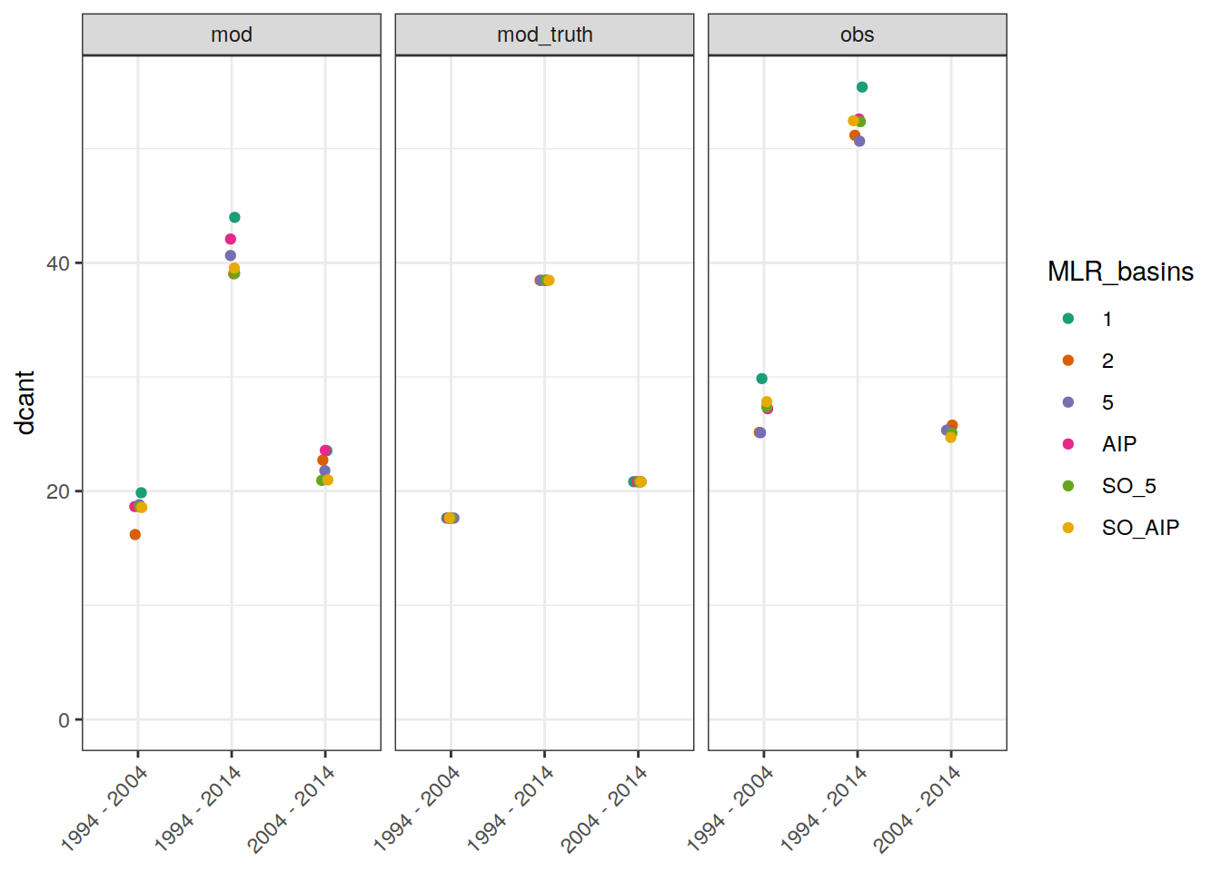

3.1.2 Biases

dcant_budget_global_bias_all %>%
  ggplot(aes(period, dcant_bias, col=MLR_basins)) +
  geom_hline(yintercept = 0) +
  scale_color_brewer(palette = "Dark2") +
  labs(y = expression(atop(Delta * C[ant] ~ bias,
                               (PgC)))) +
  geom_point() +
  theme(axis.text.x = element_blank(),
        axis.title.x = element_blank())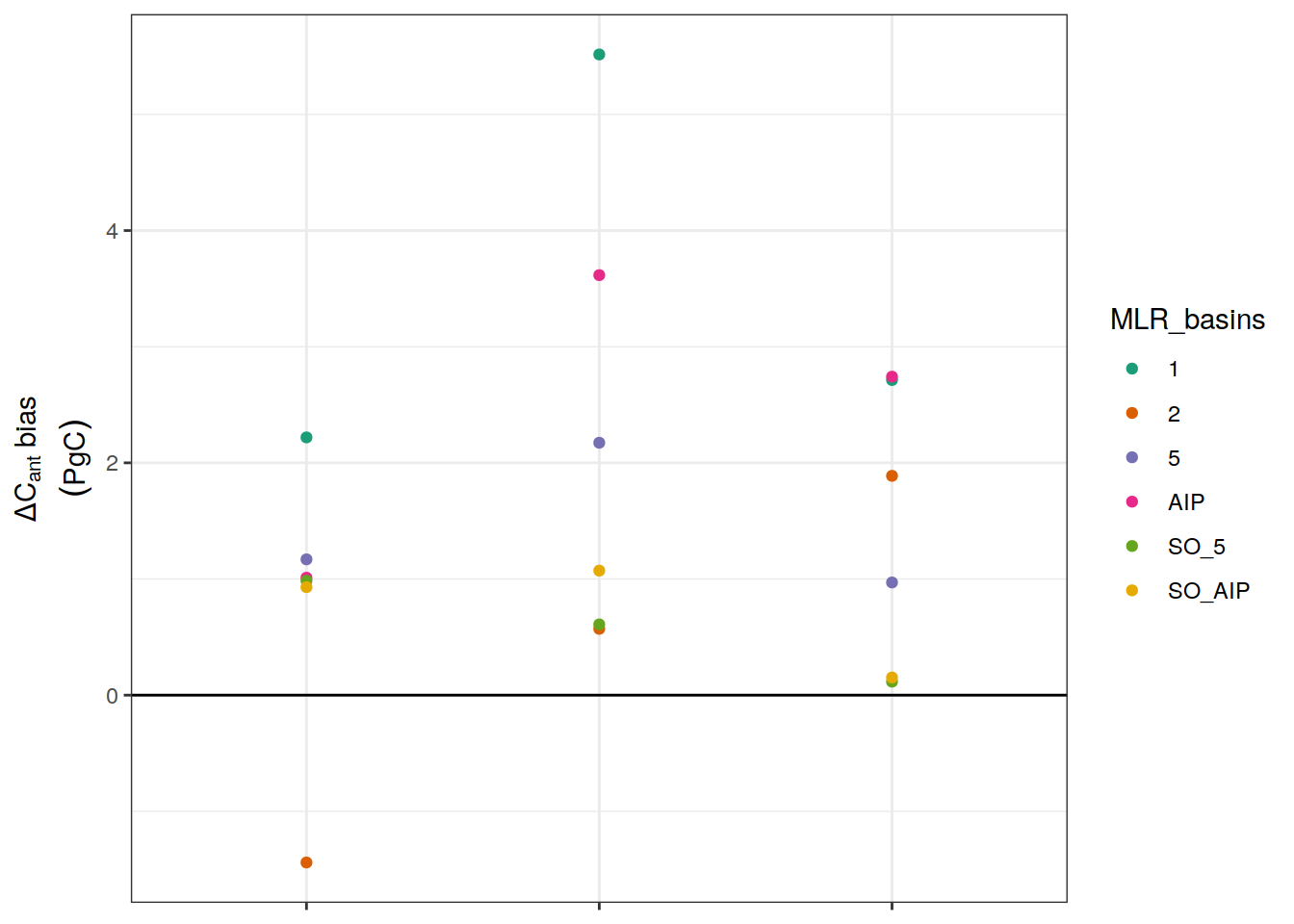

p_global_bias <-
  dcant_budget_global_bias_all %>%
  ggplot() +
  geom_hline(yintercept = global_bias_rel_max * c(-1, 1),
             linetype = 2) +
  geom_hline(yintercept = 0) +
  scale_color_brewer(palette = "Dark2") +
  labs(y = expression(Delta * C[ant] ~ bias ~ ("%")),
       title = "Model-based assesment") +
  theme(axis.title.x = element_blank()) +
  geom_point(aes(period, dcant_bias_rel, col = MLR_basins),
  alpha = 0.7) +
  theme(axis.text.x = element_text(angle = 45, hjust = 1),
        axis.title.x = element_blank())

p_global_bias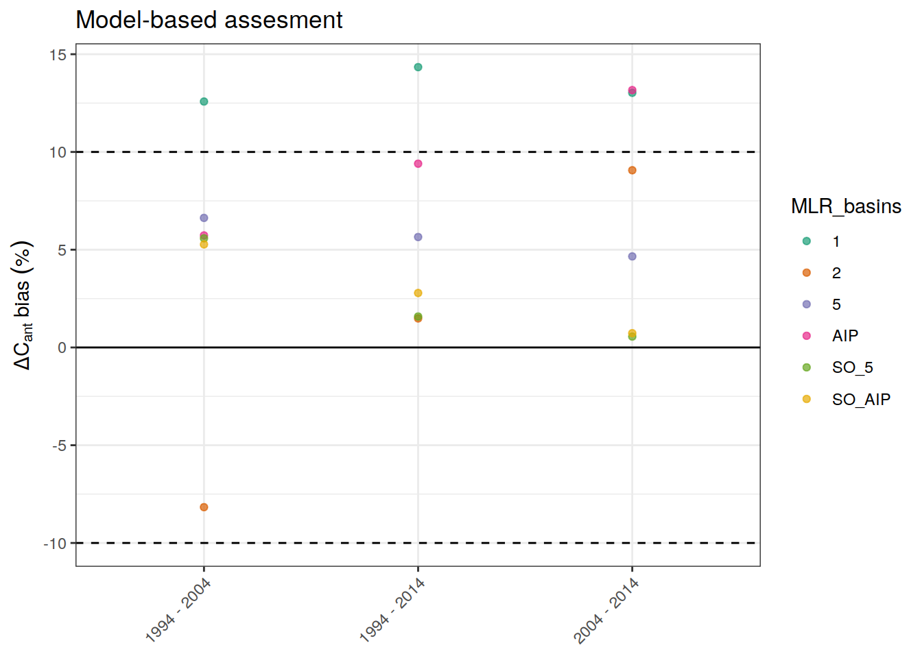

dcant_budget_global_bias_all %>%
  group_by(period) %>%
  summarise(
    dcant_bias_sd = sd(dcant_bias),
    dcant_bias = mean(dcant_bias),
    dcant_bias_rel_sd = sd(dcant_bias_rel),
    dcant_bias_rel = mean(dcant_bias_rel)
  ) %>%
  ungroup() %>%
  kable() %>%
  kable_styling() %>%
  scroll_box(height = "300px")

period	dcant_bias_sd	dcant_bias	dcant_bias_rel_sd	dcant_bias_rel
1994 - 2004	1.205534	0.8121667	6.834093	4.604119
1994 - 2014	1.971685	2.2595000	5.125520	5.873713
2004 - 2014	1.195715	1.4301667	5.740904	6.866558

3.2 Basins

3.2.1 Absoulte values

dcant_budget_basin_AIP_all %>%
  ggplot(aes(period, dcant, col = MLR_basins)) +
  geom_jitter(width = 0.05, height = 0) +
  scale_color_brewer(palette = "Dark2") +
  facet_grid(basin_AIP ~ data_source) +
  ylim(0,NA) +
  theme(axis.text.x = element_text(angle = 45, hjust=1),
        axis.title.x = element_blank())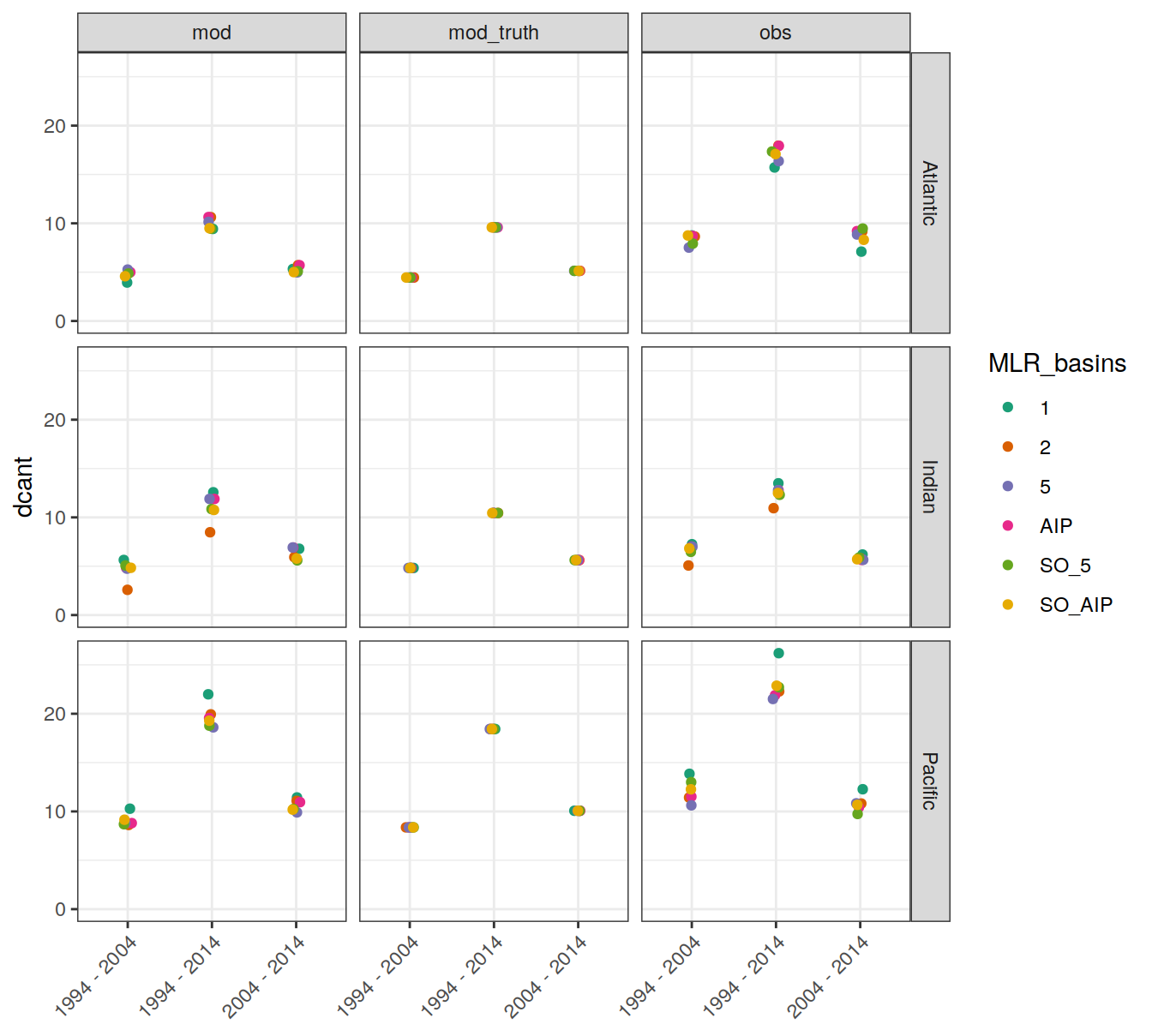

3.2.2 Biases

dcant_budget_basin_AIP_bias_all %>%
  ggplot(aes(period, dcant_bias, col=MLR_basins)) +
  geom_hline(yintercept = 0) +
  geom_point() +
  facet_grid(basin_AIP ~ .)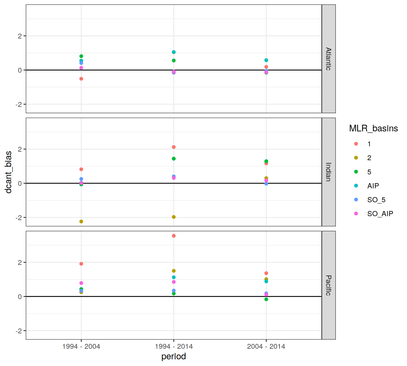

dcant_budget_basin_AIP_bias_all %>%
  ggplot() +
  geom_tile(aes(y = 0, height = regional_bias_rel_max * 2,
                x = "2004 - 2014", width = Inf,
                fill = "bias\nthreshold"), alpha = 0.5) +
  geom_hline(yintercept = 0) +
  scale_fill_manual(values = "grey70", name = "") +
  scale_color_brewer(palette = "Dark2") +
  labs(y = expression(Delta ~ C[ant] ~ bias)) +
  theme(axis.title.x = element_blank()) +
  geom_jitter(aes(period, dcant_bias_rel, col = MLR_basins),
              width = 0.05, height = 0) +
  facet_grid(. ~ basin_AIP)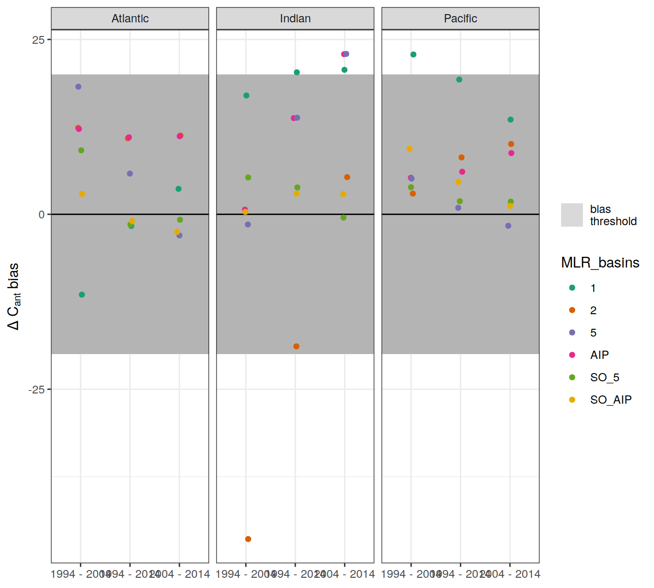

p_regional_bias <- 
  dcant_budget_basin_AIP_bias_all %>%
  ggplot() +
  geom_hline(yintercept = regional_bias_rel_max * c(-1,1),
             linetype = 2) +
  geom_hline(yintercept = 0) +
  scale_color_brewer(palette = "Dark2") +
  labs(y = expression(Delta * C[ant] ~ bias ~ ("%")),
       title = "Model-based assesment") +
  theme(axis.title.x = element_blank()) +
  geom_point(aes(period, dcant_bias_rel, col = MLR_basins),
             alpha = 0.7) +
    theme(axis.text.x = element_text(angle = 45, hjust=1),
        axis.title.x = element_blank()) +
  facet_grid(. ~ basin_AIP) +
  theme(
  strip.background = element_blank(),
  strip.text.x = element_blank()
)

p_regional_bias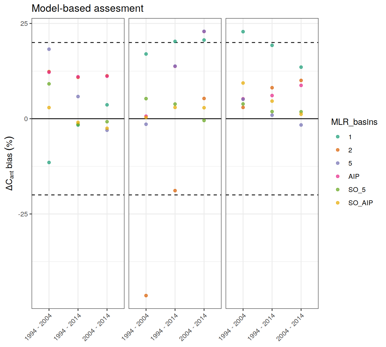

3.3 Slab budgets

3.3.1 Absolute values

dcant_slab_budget_all %>%
  filter(data_source == "obs",
         period != "1994 - 2014") %>% 
  ggplot(aes(MLR_basins, dcant, fill = gamma_slab)) +
  geom_hline(yintercept = 0, col = "red") +
  geom_col() +
  scale_fill_scico_d(direction = -1) +
  facet_grid(basin_AIP ~ period)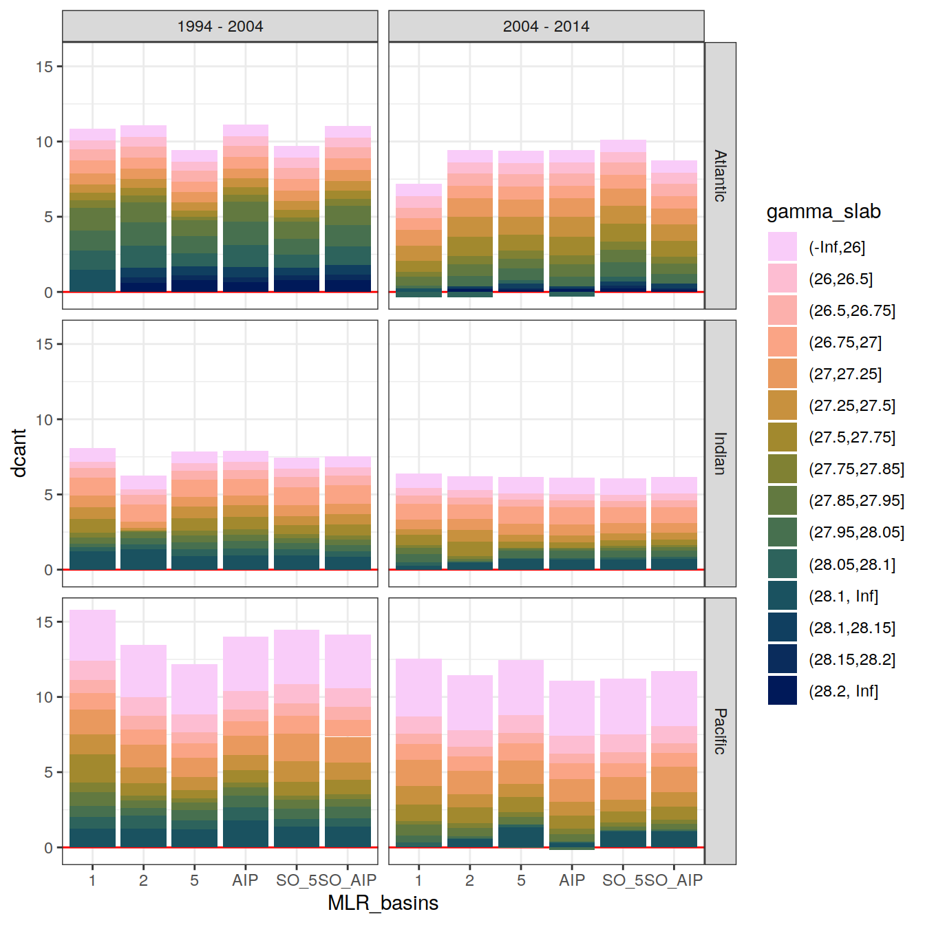

dcant_slab_budget_all %>%
  filter(data_source == "obs",
         period != "1994 - 2014") %>%
  group_by(basin_AIP) %>%
  group_split() %>%
  map(
    ~ ggplot(data = .x,
             aes(MLR_basins, dcant, fill = gamma_slab)) +
      geom_hline(yintercept = 0) +
      geom_col() +
      scale_fill_scico_d(direction = -1) +
      labs(title = paste("data_source:", unique(.x$basin_AIP))) +
      facet_grid(gamma_slab ~ period)
  )

[[1]]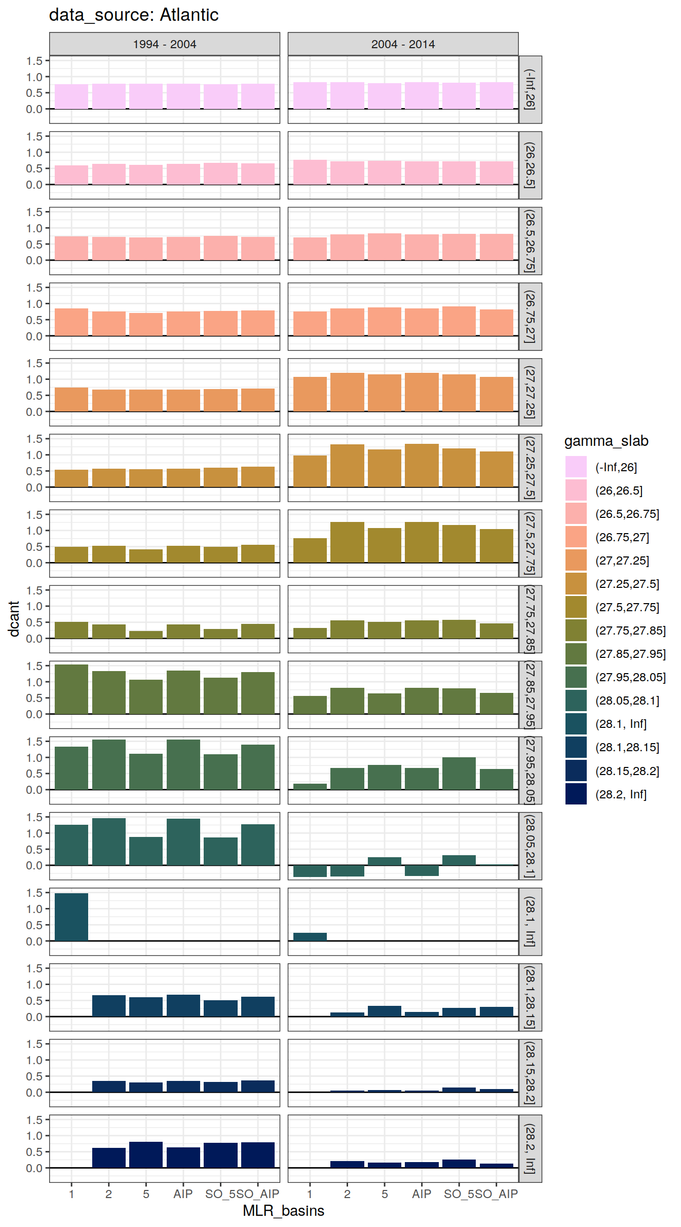

[[2]]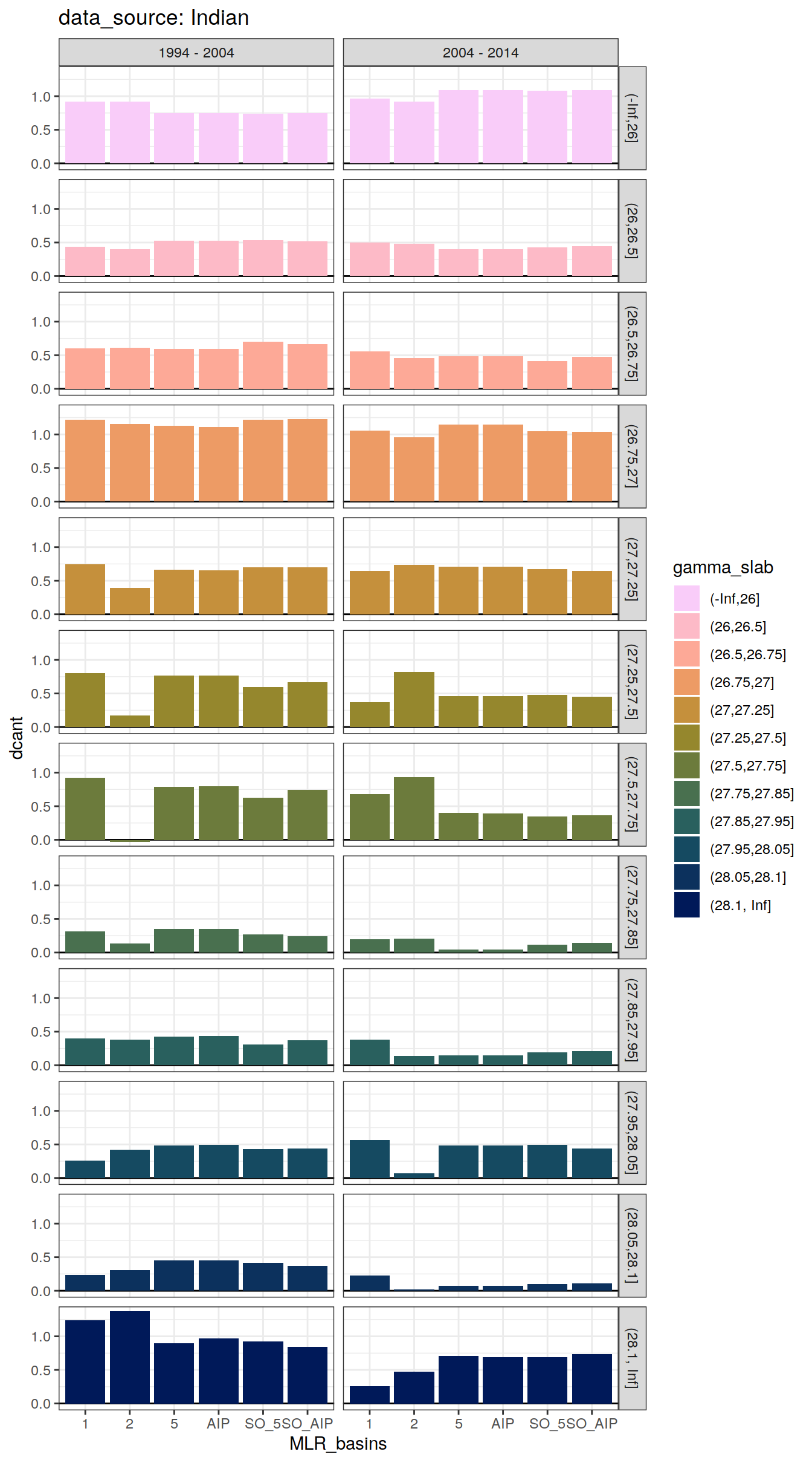

[[3]]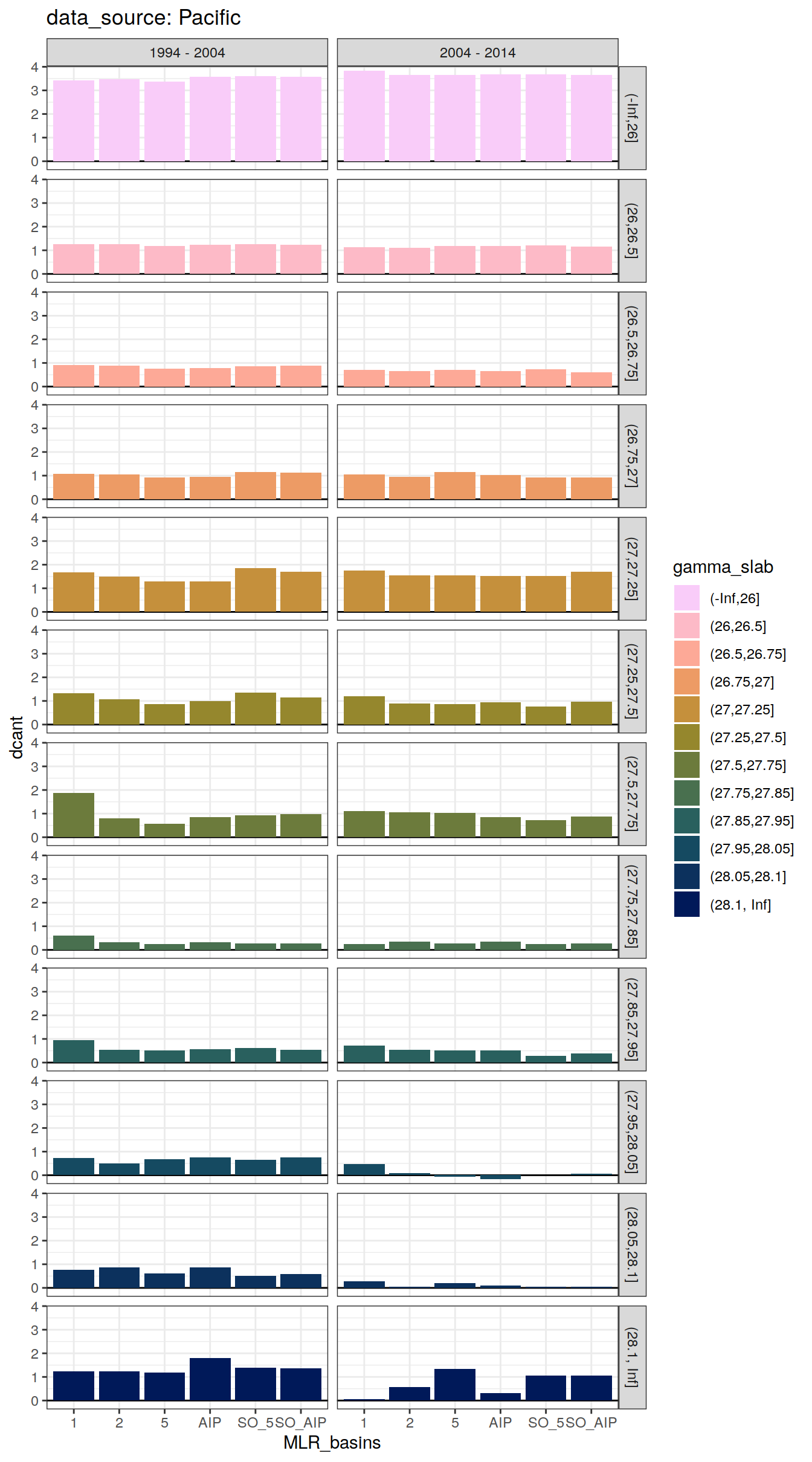

3.3.2 Bias

dcant_slab_budget_bias_all %>%
  filter(period != "1994 - 2014") %>%
  group_by(basin_AIP) %>%
  group_split() %>%
  # head(1) %>% 
  map(
    ~ ggplot(data = .x,
             aes(gamma_slab, dcant_bias, fill = gamma_slab)) +
      geom_col() +
      coord_flip() +
      scale_x_discrete(limits = rev) +
      scale_fill_scico_d(direction = -1) +
      facet_grid(period ~ MLR_basins) +
      labs(title = paste("data_source:", unique(.x$basin_AIP)))
    )

[[1]]

Warning: Removed 40 rows containing missing values (position_stack).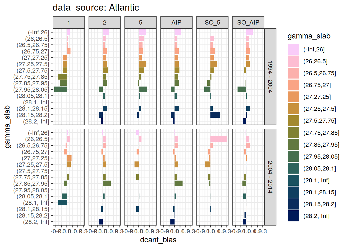

[[2]]

Warning: Removed 24 rows containing missing values (position_stack).

[[3]]

Warning: Removed 108 rows containing missing values (position_stack).

3.3.3 Spread

dcant_slab_budget_all %>%
  filter(period != "1994 - 2014",
         data_source != "mod_truth") %>%
  group_by(data_source, basin_AIP, gamma_slab, period) %>%
  summarise(dcant_range = max(dcant) - min(dcant)) %>%
  ungroup() %>%
  group_split(basin_AIP) %>%
  # head(1) %>%
  map(
    ~ ggplot(data = .x,
             aes(gamma_slab, dcant_range, fill = gamma_slab)) +
      geom_col() +
      coord_flip() +
      scale_x_discrete(limits = rev) +
      scale_fill_scico_d(direction = -1) +
      facet_grid(period ~ data_source) +
      labs(title = paste("data_source:", unique(.x$basin_AIP)))
  )

`summarise()` has grouped output by 'data_source', 'basin_AIP', 'gamma_slab'.
You can override using the `.groups` argument.

[[1]]

[[2]]

[[3]]

3.4 Basins hemisphere

3.4.1 Absoulte values

dcant_budget_basin_MLR_all %>%
  ggplot(aes(period, dcant, col = MLR_basins)) +
  geom_jitter(width = 0.05, height = 0) +
  scale_color_brewer(palette = "Dark2") +
  facet_grid(basin ~ data_source) +
  ylim(0,NA) +
  theme(axis.text.x = element_text(angle = 45, hjust=1),
        axis.title.x = element_blank())

3.4.2 Biases

dcant_budget_basin_MLR_bias_all <-
  dcant_budget_basin_MLR_all %>%
  filter(data_source %in% c("mod", "mod_truth")) %>%
  pivot_wider(names_from = data_source,
              values_from = dcant) %>%
  mutate(dcant_bias = mod - mod_truth,
         dcant_bias_rel = 100*(mod - mod_truth)/mod_truth)
  
dcant_budget_basin_MLR_bias_all %>%   
  ggplot(aes(period, dcant_bias, col=MLR_basins)) +
  geom_hline(yintercept = 0) +
  geom_point() +
  facet_grid(basin ~ .)

dcant_budget_basin_MLR_bias_all %>%
  ggplot() +
  geom_tile(aes(y = 0, height = regional_bias_rel_max * 2,
                x = "2004 - 2014", width = Inf,
                fill = "bias\nthreshold"), alpha = 0.5) +
  geom_hline(yintercept = 0) +
  scale_fill_manual(values = "grey70", name = "") +
  scale_color_brewer(palette = "Dark2") +
  labs(y = expression(Delta ~ C[ant] ~ bias)) +
  theme(axis.title.x = element_blank()) +
  geom_jitter(aes(period, dcant_bias_rel, col = MLR_basins),
              width = 0.05, height = 0) +
  facet_grid(. ~ basin)

p_regional_bias <- 
  dcant_budget_basin_MLR_bias_all %>%
  ggplot() +
  geom_hline(yintercept = regional_bias_rel_max * c(-1,1),
             linetype = 2) +
  geom_hline(yintercept = 0) +
  scale_color_brewer(palette = "Dark2") +
  labs(y = expression(Delta * C[ant] ~ bias ~ ("%")),
       title = "Model-based assesment") +
  theme(axis.title.x = element_blank()) +
  geom_point(aes(period, dcant_bias_rel, col = MLR_basins),
             alpha = 0.7) +
    theme(axis.text.x = element_text(angle = 45, hjust=1),
        axis.title.x = element_blank()) +
  facet_grid(. ~ basin) +
  theme(
  strip.background = element_blank(),
  strip.text.x = element_blank()
)

p_regional_bias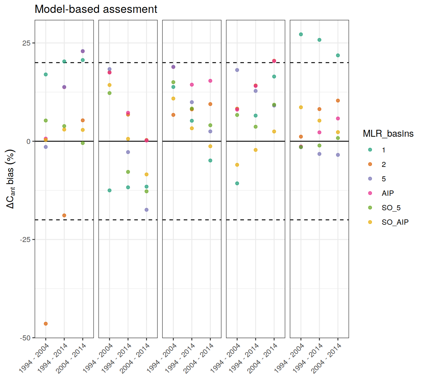

dcant_budget_basin_MLR_bias_all %>%
  group_by(period, basin) %>%
  summarise(
    dcant_bias_sd = sd(dcant_bias),
    dcant_bias = mean(dcant_bias),
    dcant_bias_rel_sd = sd(dcant_bias_rel),
    dcant_bias_rel = mean(dcant_bias_rel)
  ) %>%
  ungroup() %>%
  kable() %>%
  kable_styling() %>%
  scroll_box(height = "300px")

`summarise()` has grouped output by 'period'. You can override using the
`.groups` argument.

period	basin	dcant_bias_sd	dcant_bias	dcant_bias_rel_sd	dcant_bias_rel
1994 - 2004	Indian	1.0503048	-0.1976667	21.786037	-4.100117
1994 - 2004	N_Atlantic	0.2313883	0.2191667	11.859987	11.233555
1994 - 2004	N_Pacific	0.1287438	0.3811667	4.740199	14.034119
1994 - 2004	S_Atlantic	0.2640664	0.1016667	10.562656	4.066667
1994 - 2004	S_Pacific	0.6414012	0.3076667	11.348216	5.443501
1994 - 2014	Indian	1.4462500	0.6233333	13.842362	5.966054
1994 - 2014	N_Atlantic	0.3299485	-0.0550000	7.680365	-1.280261
1994 - 2014	N_Pacific	0.2252057	0.4790000	3.857583	8.204865
1994 - 2014	S_Atlantic	0.3531661	0.4323333	6.677369	8.174198
1994 - 2014	S_Pacific	1.3168015	0.7796667	10.453295	6.189304
2004 - 2014	Indian	0.6139226	0.6958333	10.912240	12.368172
2004 - 2014	N_Atlantic	0.1689966	-0.1943333	7.206680	-8.287136
2004 - 2014	N_Pacific	0.2286564	0.1311667	7.324037	4.201367
2004 - 2014	S_Atlantic	0.2021224	0.3633333	7.247128	13.027369
2004 - 2014	S_Pacific	0.6209901	0.4353333	8.941542	6.268299

4 Ensemble

4.1 Global

dcant_budget_global_all_in <- dcant_budget_global_all %>% 
  filter(data_source %in% c("mod", "obs"))

dcant_budget_global_ensemble <- dcant_budget_global_all_in %>% 
  group_by(data_source, period, tref2) %>% 
  summarise(dcant_mean = mean(dcant),
            dcant_sd = sd(dcant),
            dcant_range = max(dcant)- min(dcant)) %>% 
  ungroup()

`summarise()` has grouped output by 'data_source', 'period'. You can override
using the `.groups` argument.

4.1.1 Mean

legend_title = expression(Delta * C[ant]~(PgC))

ggplot() +
  geom_col(data = dcant_budget_global_ensemble,
           aes(x = period,
               y = dcant_mean),
           fill = "darkgrey") +
  geom_errorbar(
    data = dcant_budget_global_ensemble,
    aes(
      x = period,
      y = dcant_mean,
      ymax = dcant_mean + dcant_sd,
      ymin = dcant_mean - dcant_sd
    ),
    width = 0.1
  ) +
  geom_point(
    data = dcant_budget_global_all,
    aes(period, dcant, col = MLR_basins),
    alpha = 0.7,
    position = position_jitter(width = 0.2, height = 0)
  ) +
  scale_y_continuous(limits = c(0,70), expand = c(0,0)) +
  scale_color_brewer(palette = "Dark2") +
  facet_grid(. ~ data_source) +
  labs(y = legend_title) +
  theme(axis.text.x = element_text(angle = 45, hjust=1),
        axis.title.x = element_blank())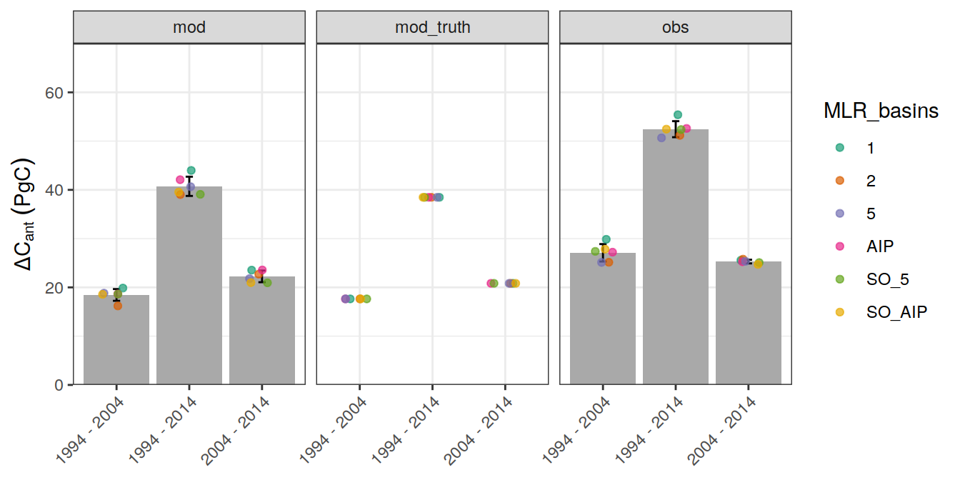

p_global_dcant <- ggplot() +
  geom_col(data = dcant_budget_global_ensemble %>% 
             filter(data_source == "obs"),
           aes(x = period,
               y = dcant_mean),
           fill = "darkgrey") +
    geom_point(
    data = dcant_budget_global_all %>% 
             filter(data_source == "obs"),
    aes(period, dcant, col = MLR_basins),
    alpha = 0.7,
    position = position_jitter(width = 0.1, height = 0)
  ) +
  geom_errorbar(
    data = dcant_budget_global_ensemble %>% 
             filter(data_source == "obs"),
    aes(
      x = period,
      y = dcant_mean,
      ymax = dcant_mean + dcant_sd,
      ymin = dcant_mean - dcant_sd
    ),
    width = 0.1
  ) +
  scale_y_continuous(limits = c(0,70), expand = c(0,0)) +
  scale_color_brewer(palette = "Dark2") +
  labs(y = legend_title,
       title = "Observation-based results") +
  theme(axis.text.x = element_blank(),
        axis.title.x = element_blank())

p_global_dcant_bias <-
p_global_dcant / p_global_bias +
  plot_layout(guides = 'collect',
              heights = c(2,1))

p_global_dcant_bias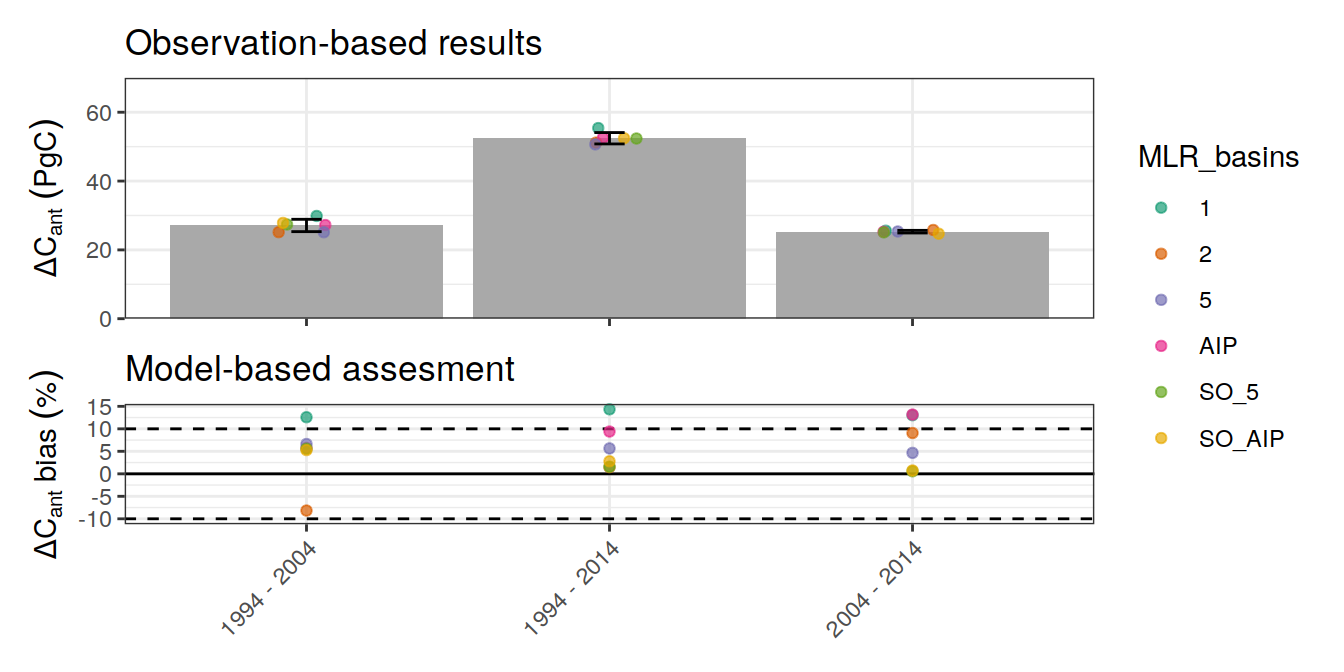

# ggsave(plot = p_global_dcant_bias,
#        path = here::here("output/publication"),
#        filename = "Fig_global_dcant_budget.png",
#        height = 5,
#        width = 5)

rm(p_global_bias, p_global_dcant, p_global_dcant_bias)

4.1.2 Mean vs atm CO2

dcant_ensemble <- dcant_budget_global_ensemble %>% 
  filter(data_source == "obs",
         period != "1994 - 2014") %>% 
  select(year = tref2, dcant_mean, dcant_sd)

tcant_S04 <- bind_cols(year = 1994, dcant_mean = 118, dcant_sd = 19)

tcant_ensemble <- full_join(dcant_ensemble, tcant_S04)

Joining, by = c("year", "dcant_mean", "dcant_sd")

tcant_ensemble <- left_join(tcant_ensemble, co2_atm)

Joining, by = "year"

co2_atm_pi <- bind_cols(pCO2 = 280, dcant_mean = 0, year = 1750, dcant_sd = 0)

tcant_ensemble <- full_join(tcant_ensemble, co2_atm_pi)

Joining, by = c("year", "dcant_mean", "dcant_sd", "pCO2")

tcant_ensemble <- tcant_ensemble %>% 
  arrange(year) %>% 
  mutate(tcant = cumsum(dcant_mean),
         tcant_sd = cumsum(dcant_sd))

tcant_ensemble %>% 
  ggplot(aes(pCO2, tcant, ymin = tcant - tcant_sd, ymax = tcant + tcant_sd)) +
  geom_ribbon(fill = "grey80") +
  geom_point() +
  geom_line() +
  scale_x_continuous(breaks = seq(280, 400, 30),
                     sec.axis = dup_axis(labels =  c(1750, 1940, 1980, 2000, 2015),
                                         name = "Year")) +
  geom_text(aes(label = year), nudge_x = -5, nudge_y = 5) +
  labs(x = expression(Atmospheric~pCO[2]~(µatm)),
       y = expression(Total~oceanic~C[ant]~(PgC)))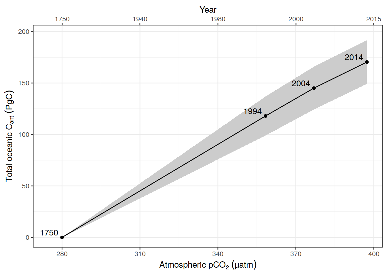

# ggsave(path = "output/publication",
#        filename = "Fig_global_dcant_budget_vs_atm_pCO2.png",
#        height = 4,
#        width = 7)

4.1.3 Sum decades

dcant_budget_global_all_in_sum <-
  dcant_budget_global_all_in %>%
  filter(period != "1994 - 2014") %>%
  arrange(tref1) %>%
  group_by(data_source, MLR_basins) %>%
  mutate(dcant = dcant + lag(dcant)) %>% 
  ungroup() %>%
  drop_na() %>% 
  mutate(estimate = "sum")

dcant_budget_global_all_in_sum <-
  bind_rows(
    dcant_budget_global_all_in_sum,
    dcant_budget_global_all_in %>%
      filter(period == "1994 - 2014") %>%
      mutate(estimate = "direct")
  )

ggplot() +
  geom_point(
    data = dcant_budget_global_all_in_sum,
    aes(estimate, dcant, col = MLR_basins),
    alpha = 0.7,
    position = position_jitter(width = 0, height = 0)
  ) +
  scale_y_continuous(limits = c(0,70), expand = c(0,0)) +
  scale_color_brewer(palette = "Dark2") +
  facet_grid(. ~ data_source) +
  theme(axis.text.x = element_text(angle = 45, hjust=1),
        axis.title.x = element_blank())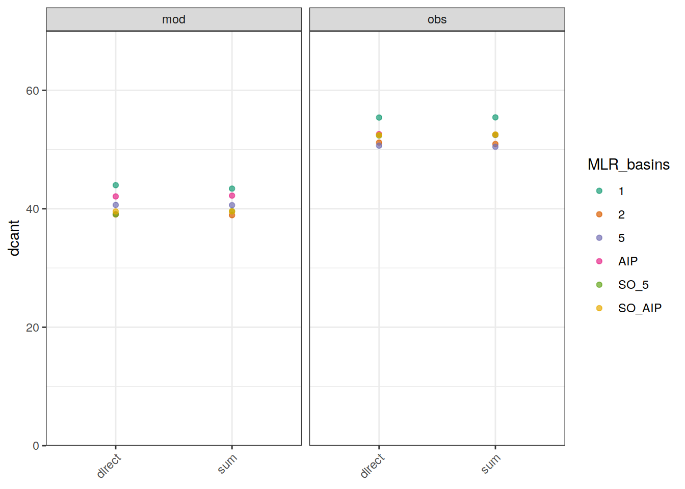

4.1.4 Mean bias

dcant_budget_global_ensemble_bias <- full_join(
  dcant_budget_global_ensemble %>%
    filter(data_source == "mod") %>% 
    select(period, dcant_mean, dcant_sd),
  dcant_budget_global_all %>%
    filter(data_source == "mod_truth",
           MLR_basins == unique(dcant_budget_global_all$MLR_basins)[1]) %>% 
    select(period, dcant)
)

Joining, by = "period"

dcant_budget_global_ensemble_bias <- dcant_budget_global_ensemble_bias %>% 
  mutate(dcant_mean_bias = dcant_mean - dcant,
         dcant_mean_bias_rel = 100 * dcant_mean_bias / dcant)

dcant_budget_global_ensemble_bias %>%
  ggplot(aes(period, dcant_mean_bias)) +
  geom_hline(yintercept = 0) +
  geom_point()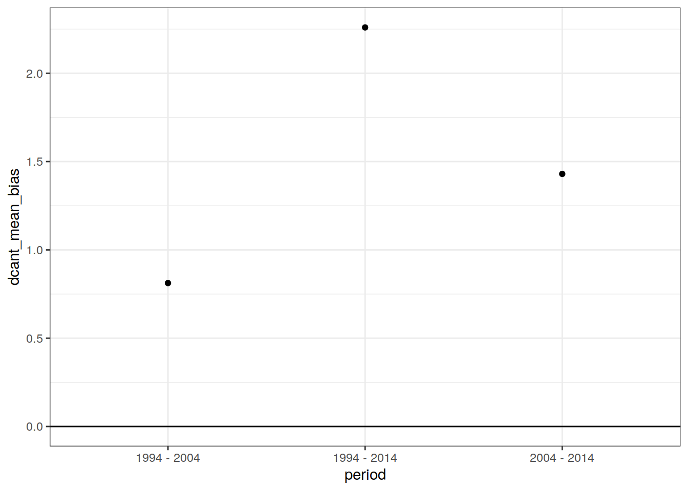

dcant_budget_global_ensemble_bias %>%
  ggplot(aes(period, dcant_mean_bias_rel)) +
  geom_hline(yintercept = 0) +
  geom_point()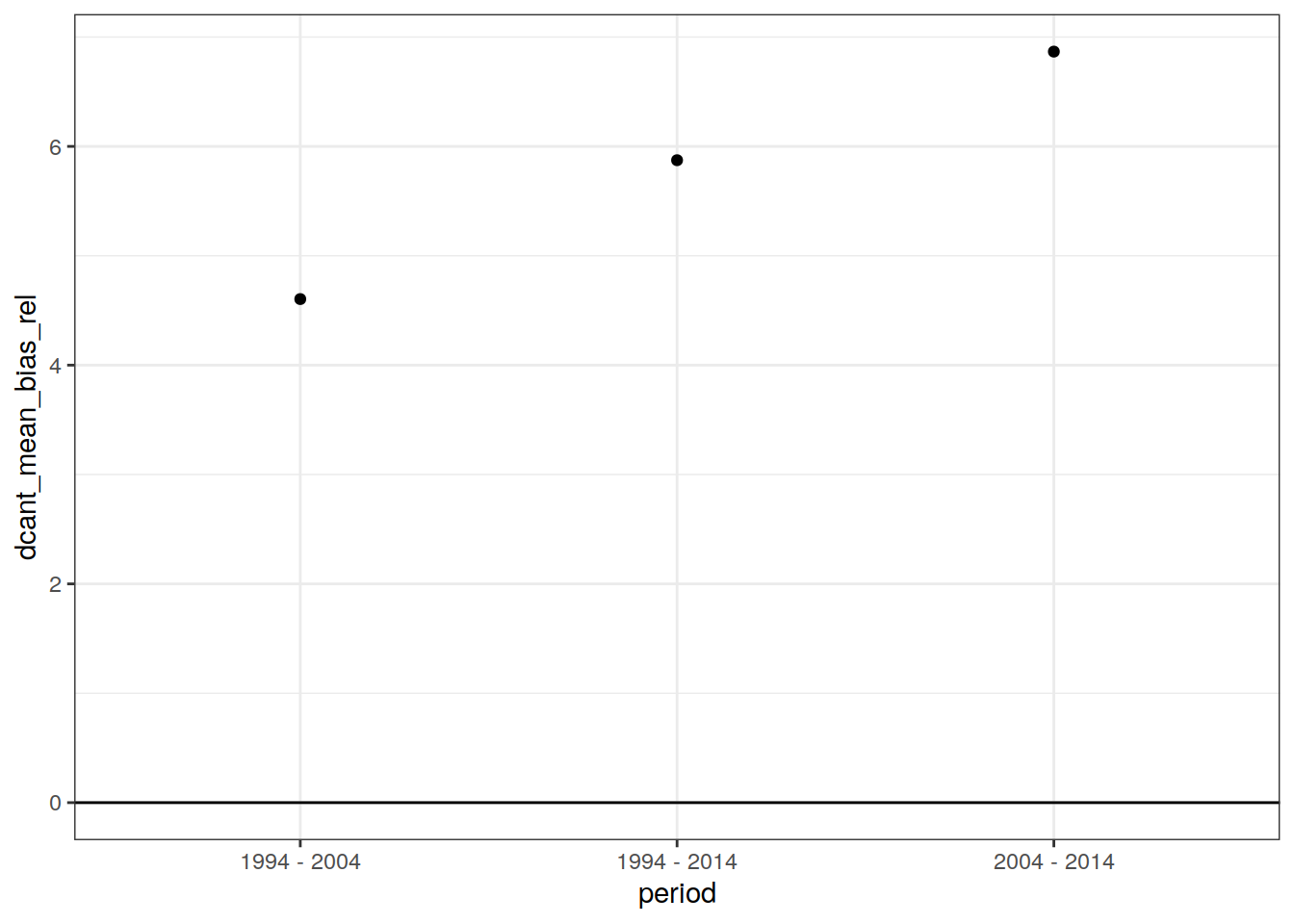

4.1.5 Vertical patterns

4.1.5.1 Absoulte values

dcant_budget_global_all_depth %>%
  filter(data_source != "mod_truth") %>% 
  group_by(data_source) %>%
  group_split() %>%
  # head(1) %>%
  map(
    ~  ggplot(data = .x,
              aes(dcant, MLR_basins, fill=period)) +
      geom_vline(xintercept = 0) +
      geom_col(position = "dodge") +
      scale_fill_brewer(palette = "Dark2") +
      facet_grid(inv_depth ~ .) +
      labs(title = paste("data_source:", unique(.x$data_source)))
  )

[[1]]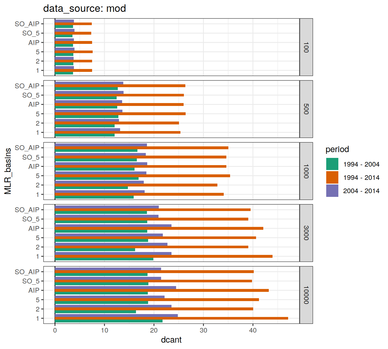

[[2]]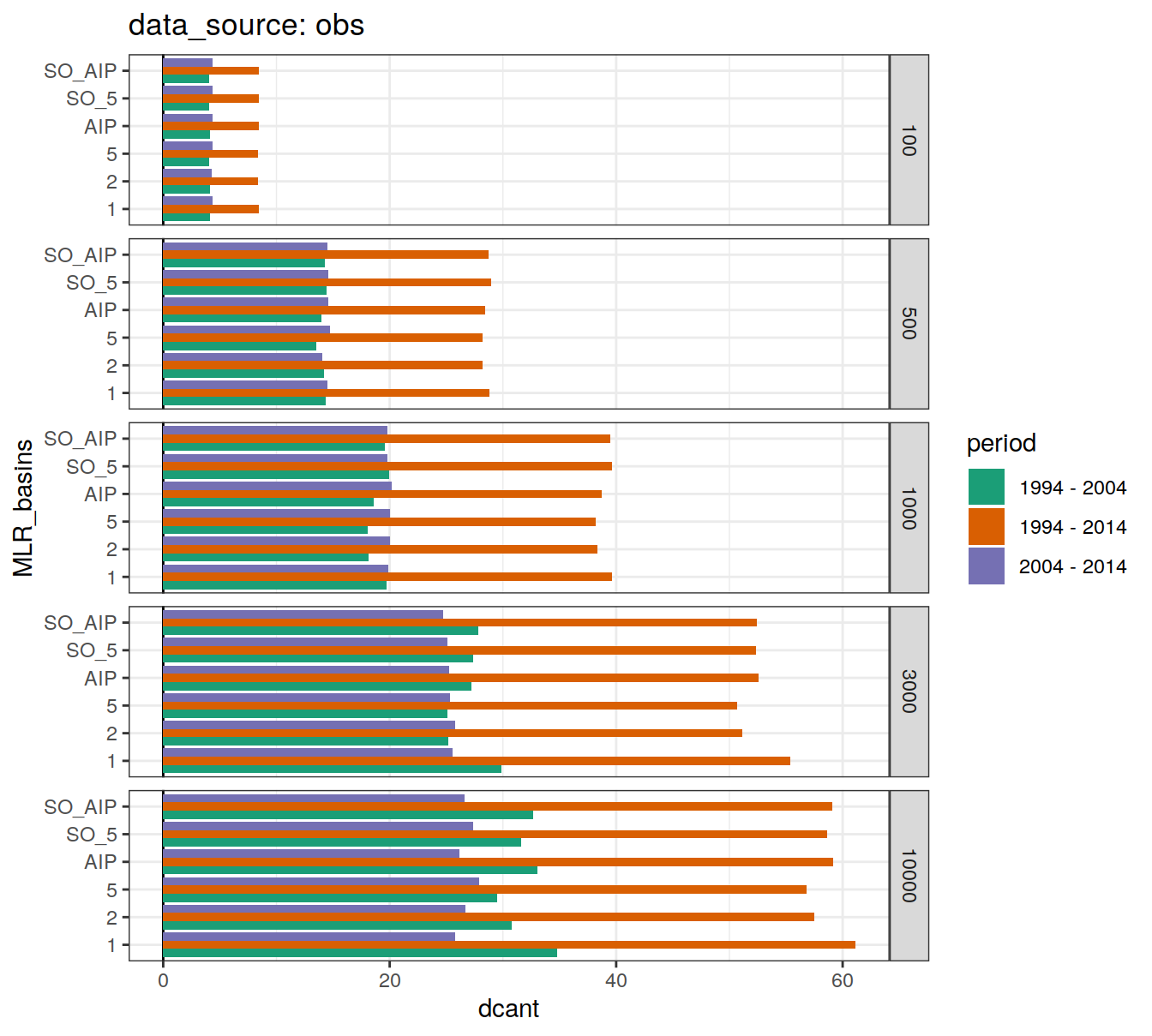

4.1.5.2 Biases

dcant_budget_global_bias_all_depth %>%
  ggplot(aes(dcant_bias, MLR_basins, fill = period)) +
  geom_vline(xintercept = 0) +
  geom_col(position = "dodge") +
  scale_fill_brewer(palette = "Dark2") +
  facet_grid(inv_depth ~ .)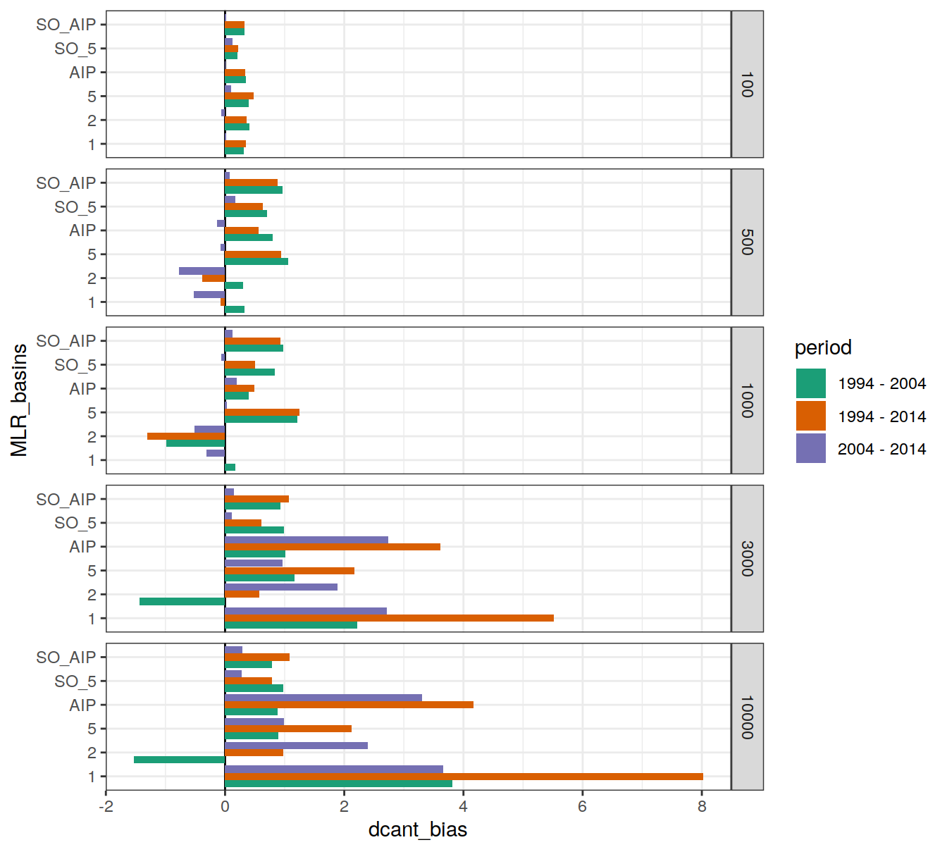

dcant_budget_global_bias_all_depth %>%
  ggplot(aes(dcant_bias_rel, MLR_basins, fill = period)) +
  geom_vline(xintercept = 0) +
  geom_col(position = "dodge") +
  scale_fill_brewer(palette = "Dark2") +
  facet_grid(inv_depth ~ .)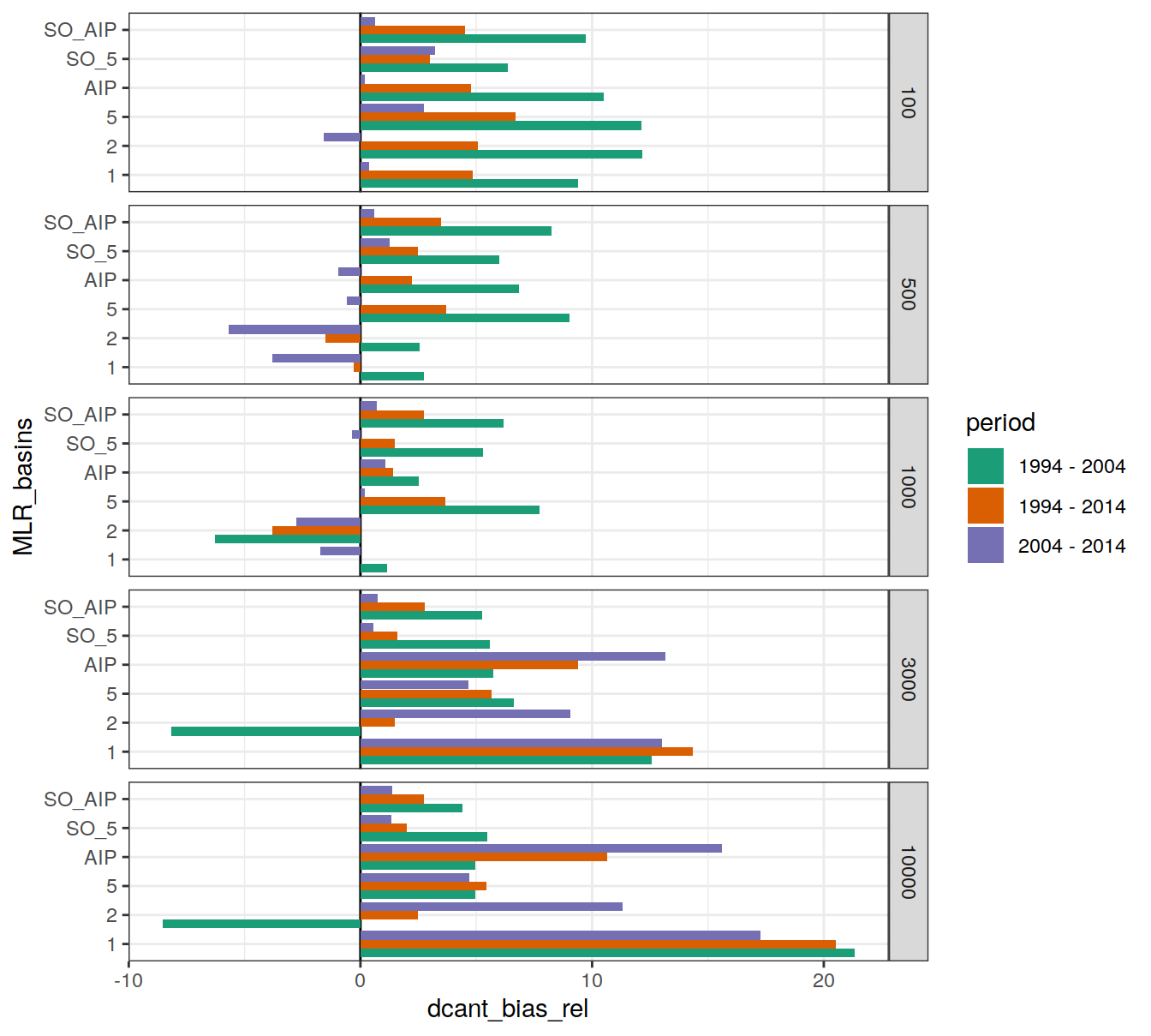

rm(dcant_budget_global_all,
   dcant_budget_global_all_depth,
   dcant_budget_global_bias_all,
   dcant_budget_global_bias_all_depth,
   dcant_budget_global_ensemble,
   dcant_budget_global_ensemble_bias)

4.2 Basins

dcant_budget_basin_AIP_ensemble <- dcant_budget_basin_AIP_all %>% 
  filter(data_source %in% c("mod", "obs")) %>% 
  group_by(basin_AIP, data_source, period) %>% 
  summarise(dcant_mean = mean(dcant),
            dcant_sd = sd(dcant),
            dcant_range = max(dcant)- min(dcant)) %>% 
  ungroup()

`summarise()` has grouped output by 'basin_AIP', 'data_source'. You can override
using the `.groups` argument.

4.2.1 Mean

dcant_budget_basin_AIP_ensemble %>%
  ggplot(aes(period, dcant_mean, col=basin_AIP)) +
  geom_pointrange(aes(ymax = dcant_mean + dcant_sd,
                      ymin = dcant_mean - dcant_sd),
                  shape = 21) +
  facet_grid(. ~ data_source)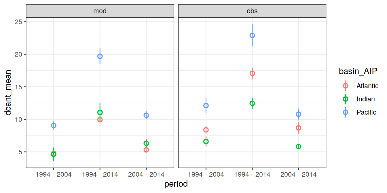

p_regional_dcant <- ggplot() +
  geom_col(
    data = dcant_budget_basin_AIP_ensemble %>%
      filter(data_source == "obs"),
    aes(x = period,
        y = dcant_mean),
    fill = "darkgrey"
  ) +
  geom_point(
    data = dcant_budget_basin_AIP_all %>%
      filter(data_source == "obs"),
    aes(period, dcant, col = MLR_basins),
    position = position_jitter(width = 0.1, height = 0),
    alpha = 0.7
  ) +
  geom_errorbar(
    data = dcant_budget_basin_AIP_ensemble %>%
      filter(data_source == "obs"),
    aes(
      x = period,
      y = dcant_mean,
      ymax = dcant_mean + dcant_sd,
      ymin = dcant_mean - dcant_sd
    ),
    width = 0.1
  ) +
  scale_y_continuous(limits = c(0, 35), expand = c(0, 0)) +
  scale_color_brewer(palette = "Dark2") +
  labs(y = legend_title,
       title = "Observation-based results") +
  theme(axis.text.x = element_blank(),
        axis.title.x = element_blank()) +
  facet_grid(. ~ basin_AIP)

p_regional_dcant_bias <-
p_regional_dcant / p_regional_bias +
  plot_layout(guides = 'collect',
              heights = c(2,1))

p_regional_dcant_bias

# ggsave(plot = p_regional_dcant_bias,
#        path = "output/publication",
#        filename = "Fig_regional_dcant_budget.png",
#        height = 5,
#        width = 10)

rm(p_regional_bias, p_regional_dcant, p_regional_dcant_bias)

4.2.2 Mean bias

dcant_budget_basin_AIP_ensemble_bias <- full_join(
  dcant_budget_basin_AIP_ensemble %>%
    filter(data_source == "mod") %>% 
    select(basin_AIP, period, dcant_mean, dcant_sd),
  dcant_budget_basin_AIP_all %>%
    filter(data_source == "mod_truth",
           MLR_basins == unique(dcant_budget_basin_AIP_all$MLR_basins)[1]) %>% 
    select(basin_AIP, period, dcant)
)

Joining, by = c("basin_AIP", "period")

dcant_budget_basin_AIP_ensemble_bias <- dcant_budget_basin_AIP_ensemble_bias %>% 
  mutate(dcant_mean_bias = dcant_mean - dcant,
         dcant_mean_bias_rel = 100 * dcant_mean_bias / dcant)


dcant_budget_basin_AIP_ensemble_bias %>%
  ggplot(aes(period, dcant_mean_bias, col = basin_AIP)) +
  geom_hline(yintercept = 0) +
  geom_point()

dcant_budget_basin_AIP_ensemble_bias %>%
  ggplot(aes(period, dcant_mean_bias_rel, col = basin_AIP)) +
  geom_hline(yintercept = 0) +
  geom_point()

4.2.3 Vertical patterns

4.2.3.1 Absoulte values

dcant_budget_basin_AIP_all_depth %>%
  filter(data_source != "mod_truth") %>%
  group_by(data_source) %>%
  group_split() %>%
  # head(1) %>%
  map(
    ~  ggplot(data = .x,
              aes(dcant, MLR_basins, fill = basin_AIP)) +
      geom_vline(xintercept = 0) +
      geom_col() +
      scale_fill_brewer(palette = "Dark2") +
      facet_grid(inv_depth ~ period) +
      labs(title = paste("data_source:", unique(.x$data_source)))
  )

[[1]]

[[2]]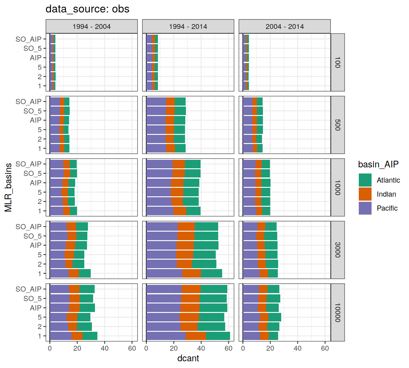

4.2.3.2 Biases

dcant_budget_basin_AIP_bias_all_depth %>%
  ggplot(aes(dcant_bias, MLR_basins, fill = basin_AIP)) +
  geom_vline(xintercept = 0) +
  geom_col() +
  scale_fill_brewer(palette = "Dark2") +
  facet_grid(inv_depth ~ period)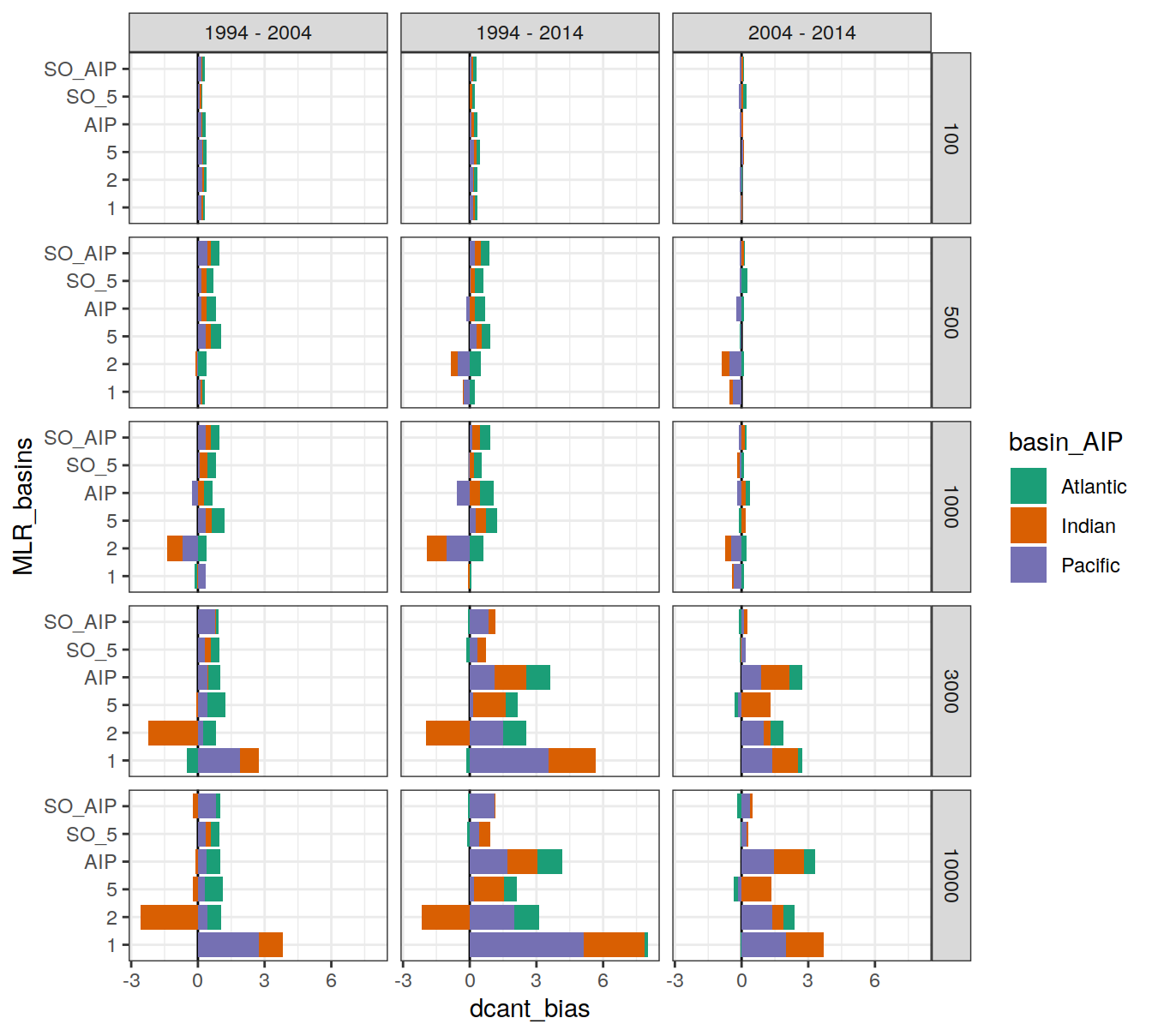

dcant_budget_basin_AIP_bias_all_depth %>%
  ggplot(aes(dcant_bias_rel, MLR_basins, fill = basin_AIP)) +
  geom_vline(xintercept = 0) +
  geom_col(position = "dodge") +
  scale_fill_brewer(palette = "Dark2") +
  facet_grid(inv_depth ~ period)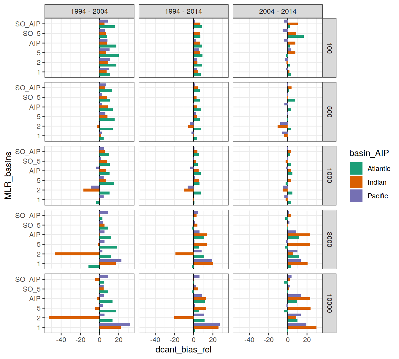

5 Steady state

dcant_obs_budget_all %>%
  group_by(inv_depth) %>%
  group_split() %>%
  # head(1) %>% 
  map(
    ~ ggplot(data = .x,
             aes(estimate, dcant_pos, fill = basin_AIP)) +
      scale_fill_brewer(palette = "Dark2") +
      geom_col() +
      facet_grid(MLR_basins ~ period) +
      labs(title = paste("inventory depth:",unique(.x$inv_depth)))
  )

[[1]]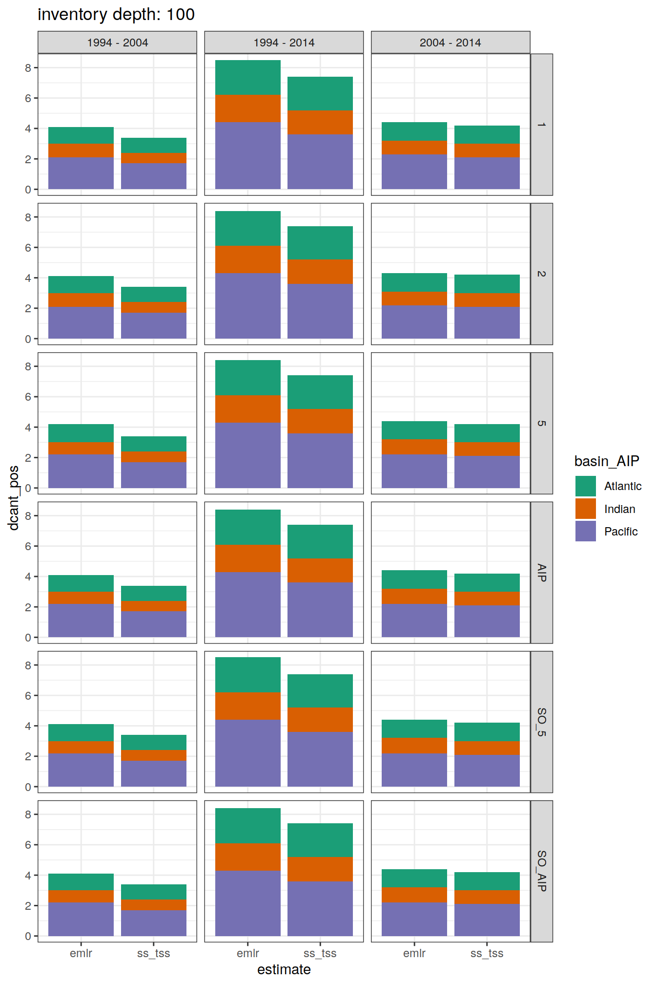

[[2]]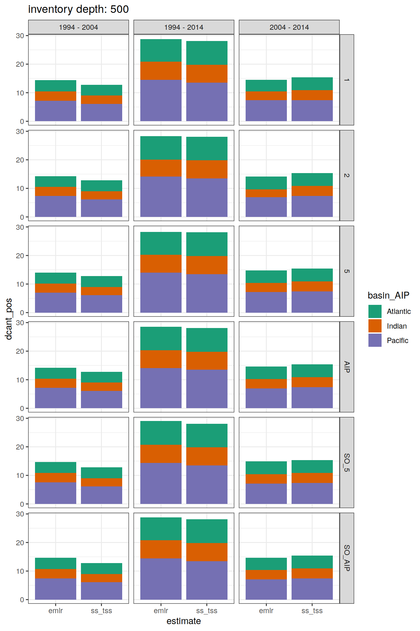

[[3]]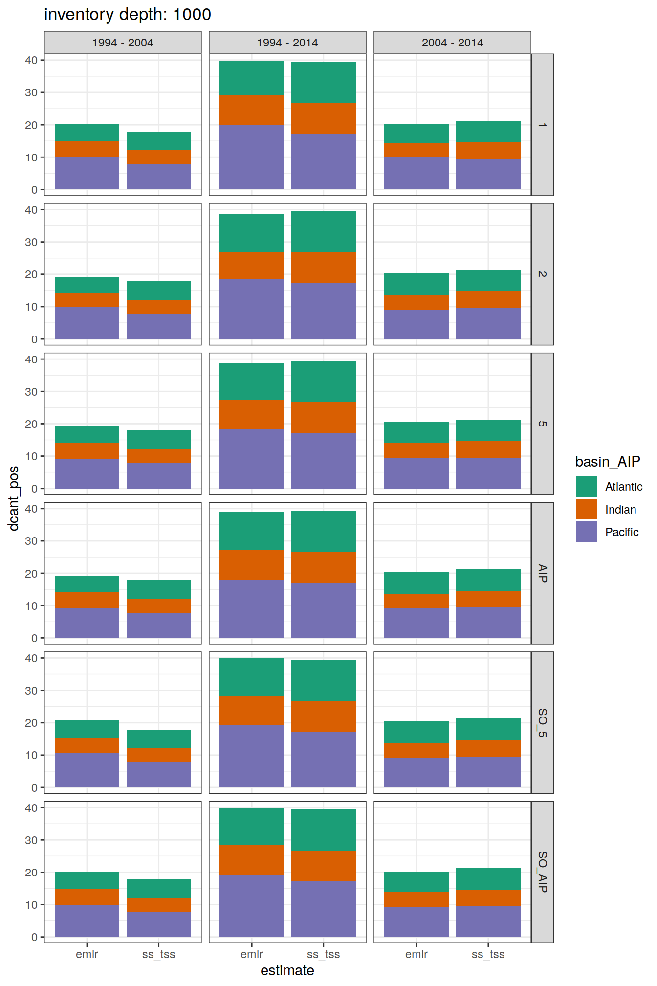

[[4]]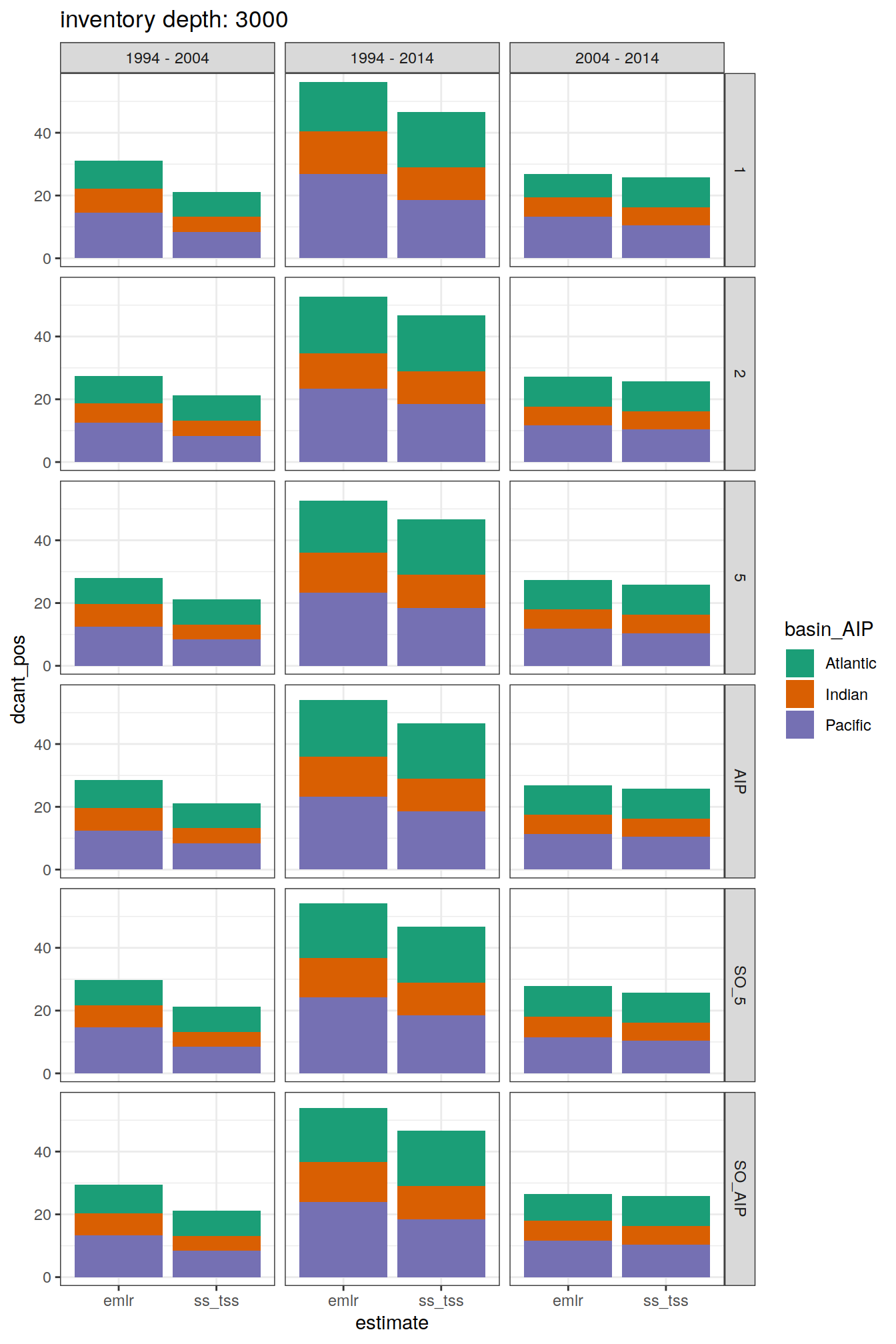

[[5]]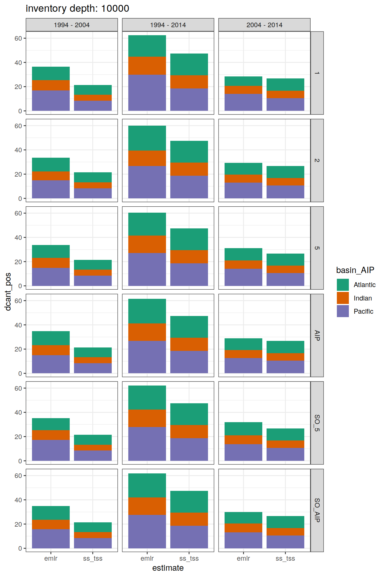

6 Predictor analysis

lm_best_predictor_counts_all <-
  full_join(lm_best_predictor_counts_all,
            params_local_all)

Joining, by = "Version_ID"

lm_best_predictor_counts_all <- lm_best_predictor_counts_all %>% 
  mutate(n_predictors_total = rowSums(across(aou:temp), na.rm = TRUE)/10)

lm_best_predictor_counts_all %>%
  ggplot(aes(x = MLR_basins, y = n_predictors_total)) +
  # ggdist::stat_halfeye(
  #   adjust = .5,
  #   width = .6,
  #   .width = 0,
  #   justification = -.2,
  #   point_colour = NA
  # ) +
  geom_boxplot(width = 0.5,
               outlier.shape = NA) +
  gghalves::geom_half_point(
    side = "l",
    range_scale = .4,
    alpha = .5,
    aes(col = gamma_slab)
  ) +
  scale_color_viridis_d() +
  facet_grid(basin ~ data_source)

lm_best_predictor_counts_all %>%
  pivot_longer(aou:temp,
               names_to = "predictor",
               values_to = "count") %>%
  group_split(predictor) %>%
  # head(1) %>%
  map(
    ~ ggplot(data = .x,
             aes(MLR_basins, count, color = gamma_slab)) +
      geom_jitter(alpha = 0.5) +
      scale_color_viridis_d() +
      labs(title = paste0("predictor:", unique(.x$predictor))) +
      coord_cartesian(ylim = c(0, 10)) +
      facet_grid(basin ~ data_source)
  )

[[1]]

[[2]]

Warning: Removed 23 rows containing missing values (geom_point).

[[3]]

Warning: Removed 2 rows containing missing values (geom_point).

[[4]]

Warning: Removed 23 rows containing missing values (geom_point).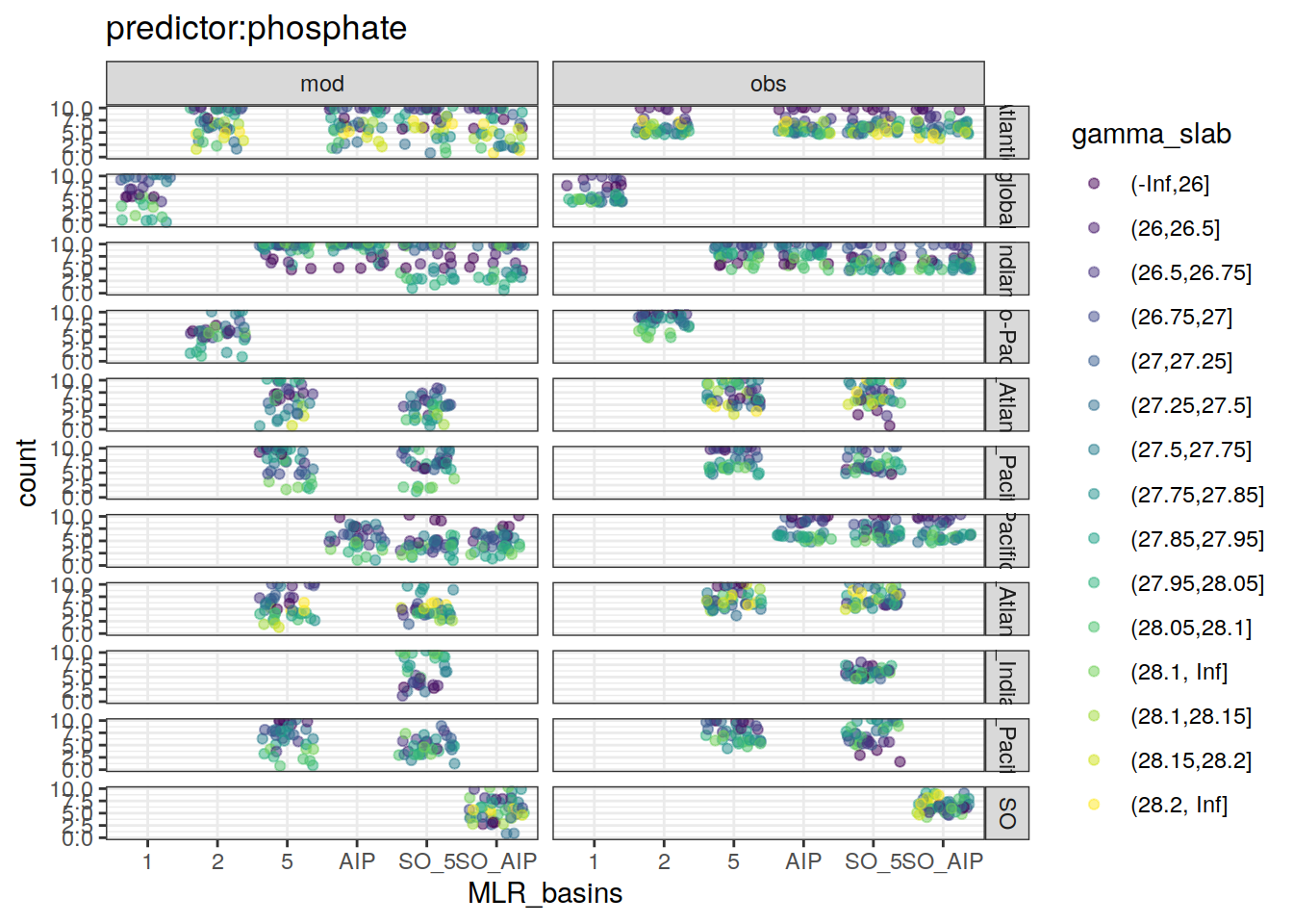

[[5]]

Warning: Removed 5 rows containing missing values (geom_point).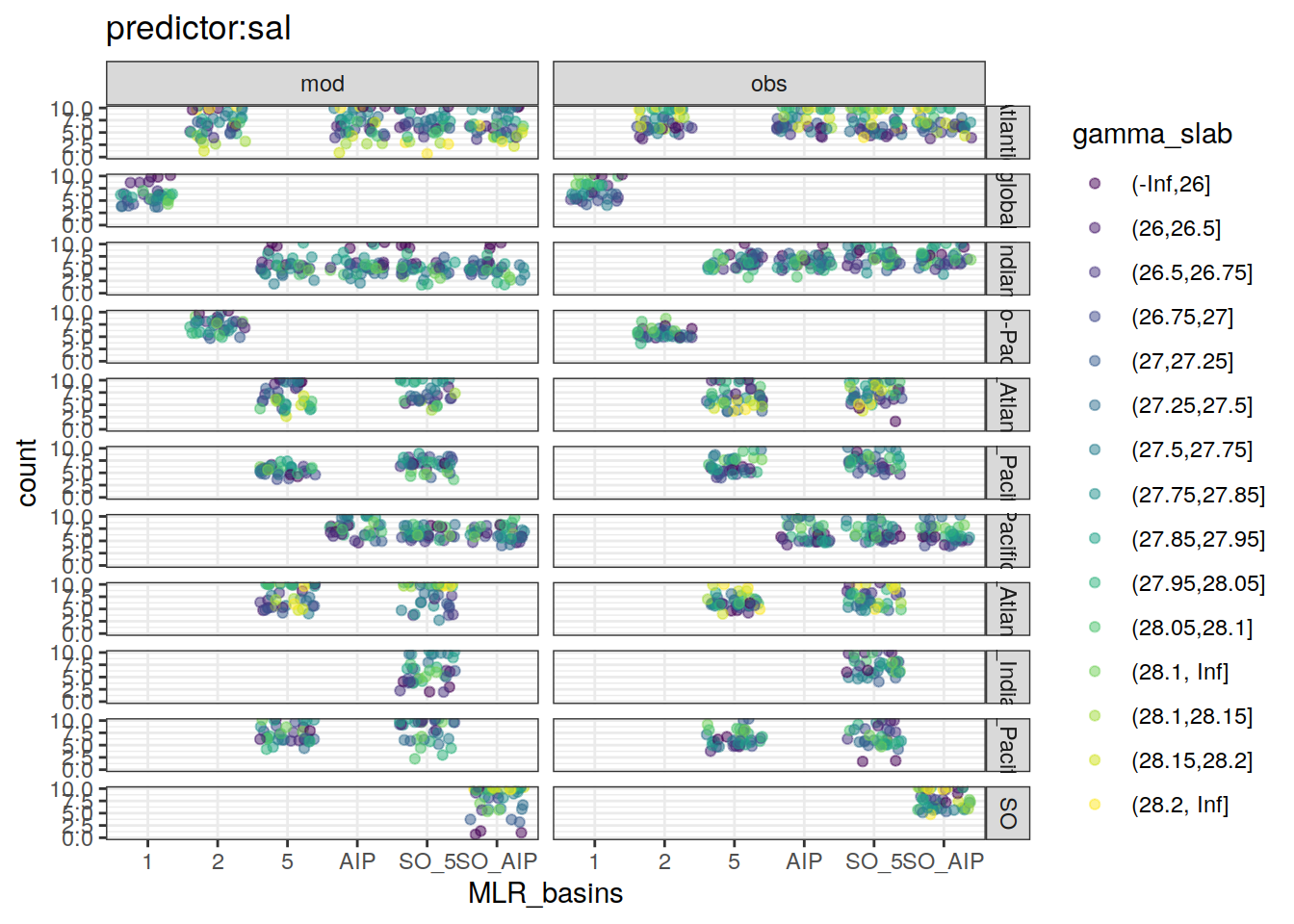

[[6]]

Warning: Removed 6 rows containing missing values (geom_point).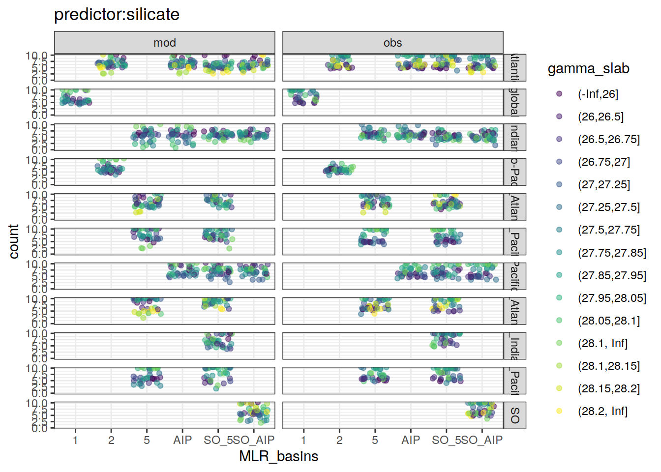

[[7]]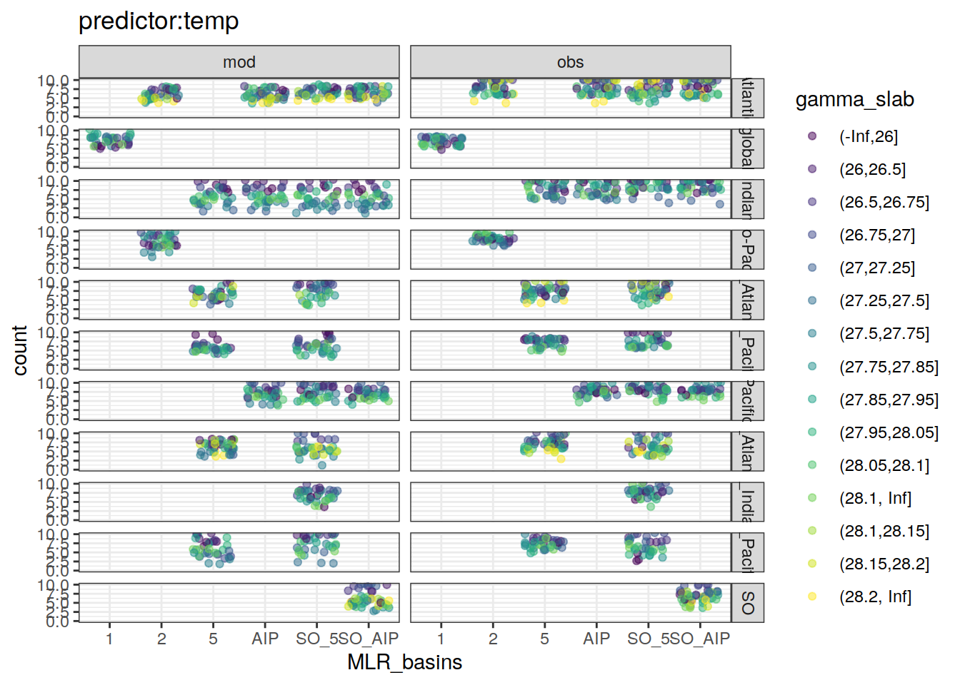

lm_best_dcant_all <-
  full_join(lm_best_dcant_all,
            params_local_all)

Joining, by = "Version_ID"

lm_best_dcant_all %>%
  count(basin, data_source, gamma_slab, MLR_basins, period) %>%
  ggplot(aes(MLR_basins, n)) +
  geom_jitter(height = 0, alpha = 0.3) +
  facet_grid(basin ~ data_source)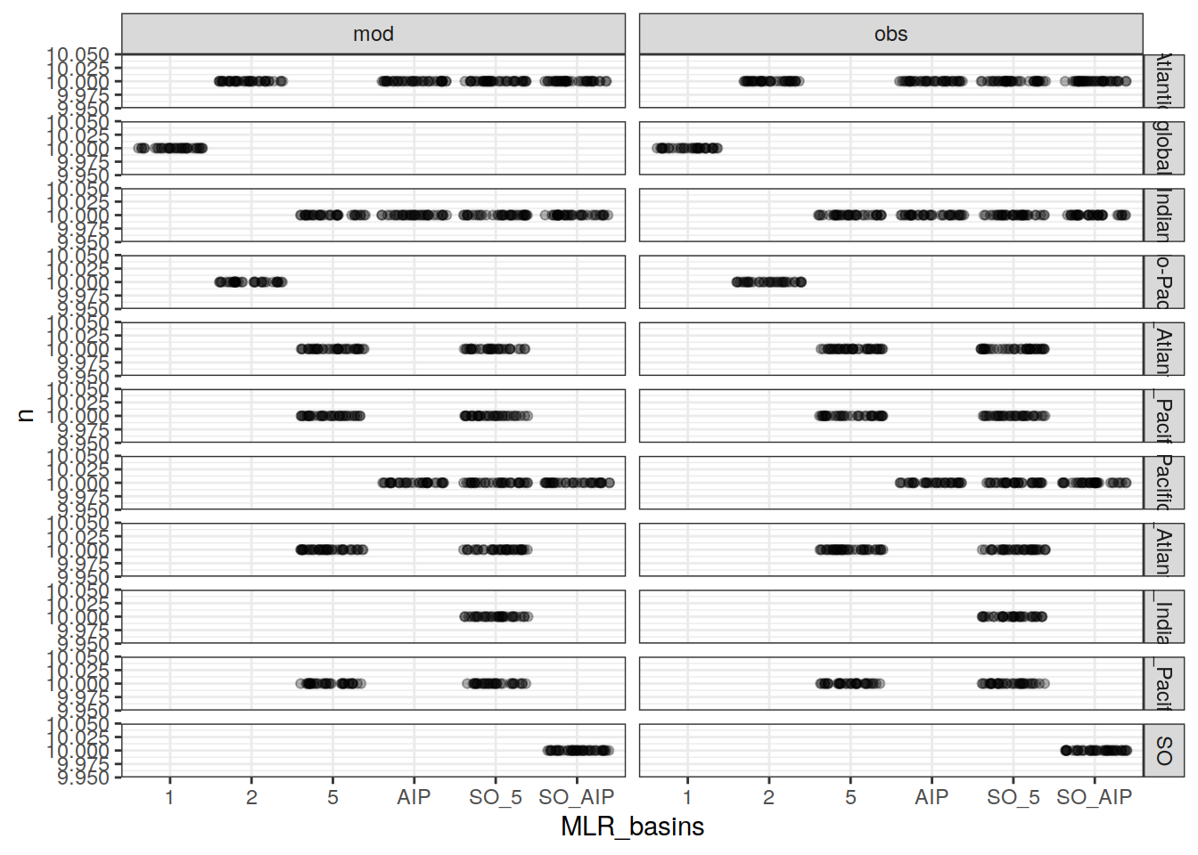

7 Drift and bias

dcant_budget_global_all_dissic %>%
  filter(estimate == "dcant") %>%
  ggplot(aes(inv_depth, value, col = !!sym(config))) +
  geom_hline(yintercept = 0) +
  scale_color_brewer(palette = "Dark2") +
  geom_point() +
  geom_path() +
  labs(y = "DIC change (PgC)") +
  facet_grid(data_source ~ period, scales = "free_y")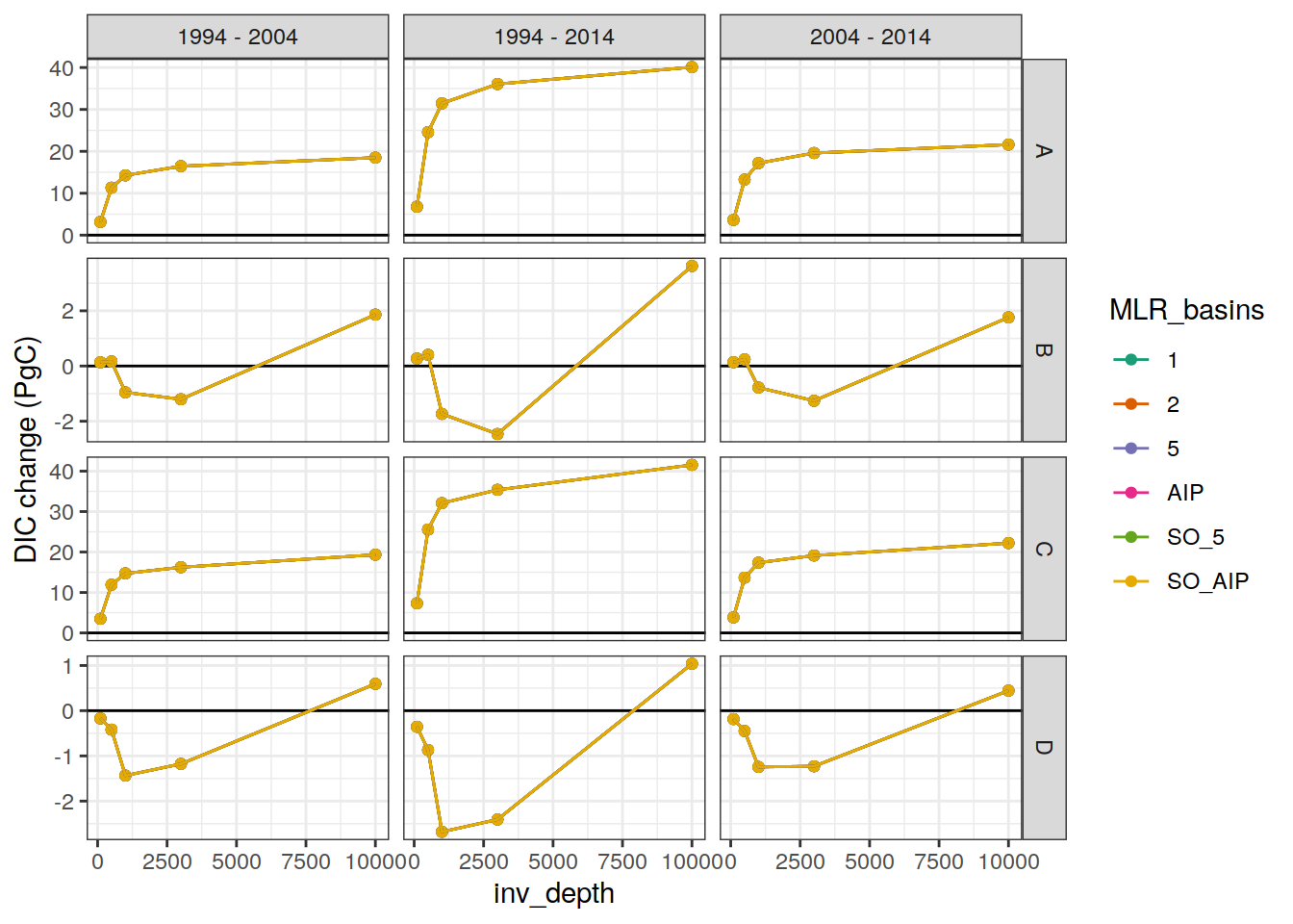

dcant_budget_global_bias_all_decomposition <-
  dcant_budget_global_bias_all_decomposition %>%
  filter(estimate == "dcant") %>%
  select(inv_depth, dcant_bias, contribution, !!sym(config), period) %>%
  pivot_wider(names_from = contribution,
              values_from = dcant_bias)

dcant_budget_global_bias_all_decomposition <-
  full_join(
    dcant_budget_global_bias_all_decomposition,
    dcant_budget_global_bias_all_depth %>%
      select(inv_depth, !!sym(config), period, mod_truth)
  )

Joining, by = c("inv_depth", "MLR_basins", "period")

dcant_budget_global_bias_all_decomposition %>%
  ggplot(aes(`dcant offset`, `delta C* - mod_truth`, col = !!sym(config))) +
  geom_vline(xintercept = 0, col = "grey50") +
  geom_hline(yintercept = 0, col = "grey50") +
  geom_abline(intercept = 0, slope = 1) +
  geom_point() +
  coord_fixed() +
  scale_color_brewer(palette = "Dark2") +
  facet_grid(inv_depth ~ period)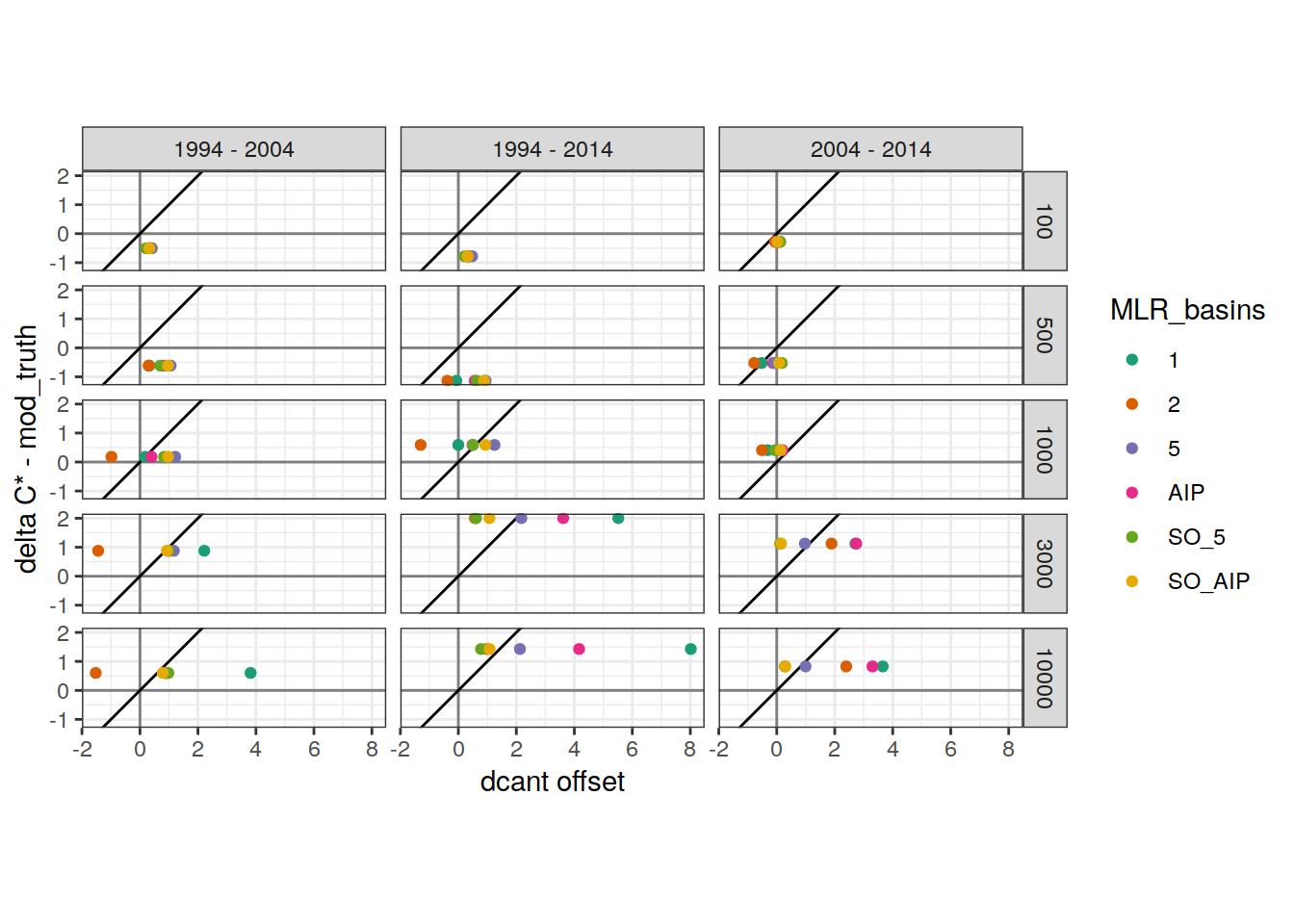

dcant_budget_global_bias_all_decomposition %>%
  ggplot(aes(`dcant offset`, `C* prediction error`, col = !!sym(config))) +
  geom_vline(xintercept = 0, col = "grey50") +
  geom_hline(yintercept = 0, col = "grey50") +
  geom_abline(intercept = 0, slope = 1) +
  geom_point() +
  coord_fixed() +
  scale_color_brewer(palette = "Dark2") +
  facet_grid(inv_depth ~ period)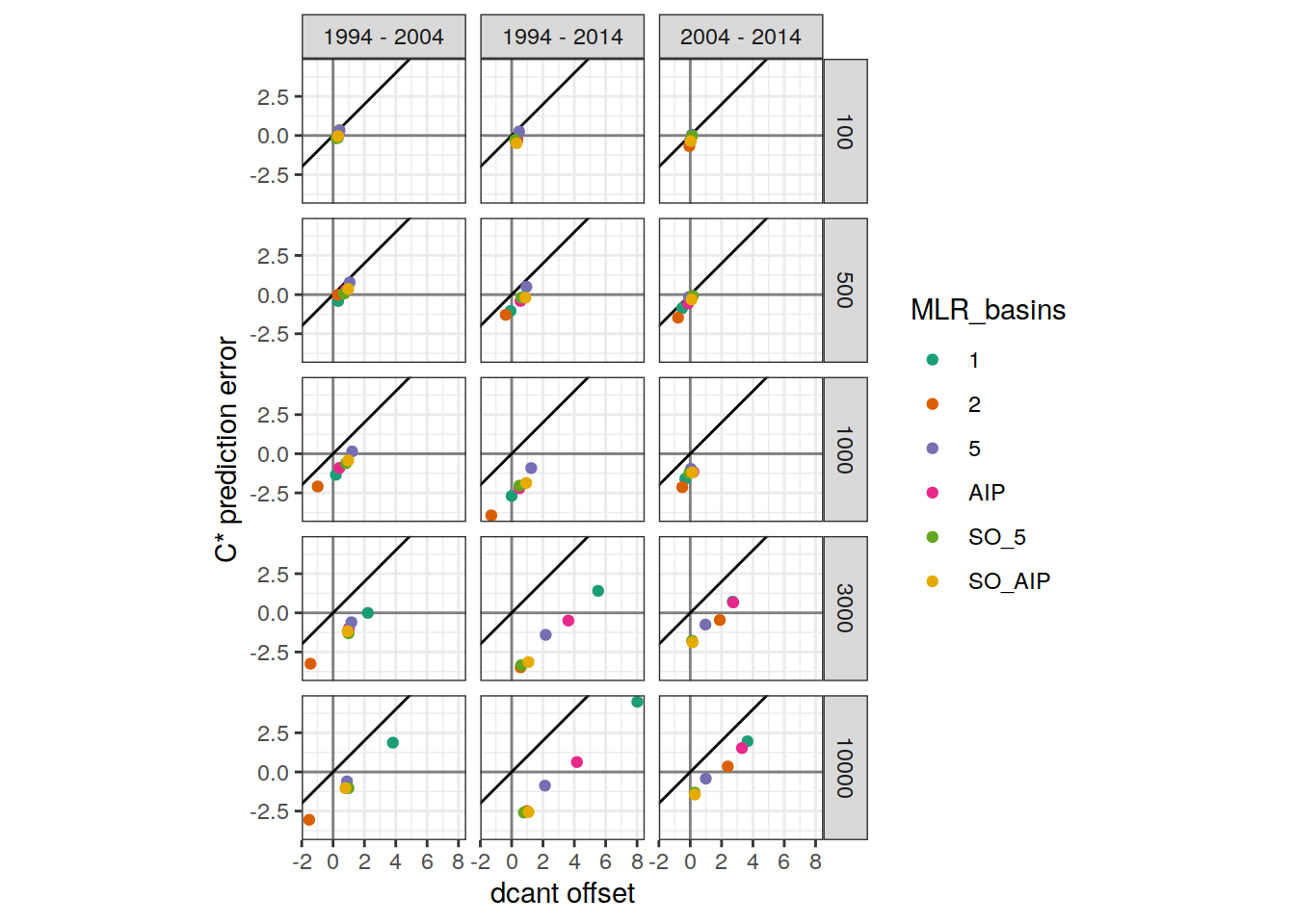

dcant_budget_global_bias_all_decomposition %>%
  ggplot(aes(
    `dcant offset`,
    `C* prediction error` + `delta C* - mod_truth`,
    col = !!sym(config)
  )) +
  geom_vline(xintercept = 0, col = "grey50") +
  geom_hline(yintercept = 0, col = "grey50") +
  geom_abline(intercept = 0, slope = 1) +
  geom_point() +
  coord_fixed() +
  scale_color_brewer(palette = "Dark2") +
  facet_grid(inv_depth ~ period)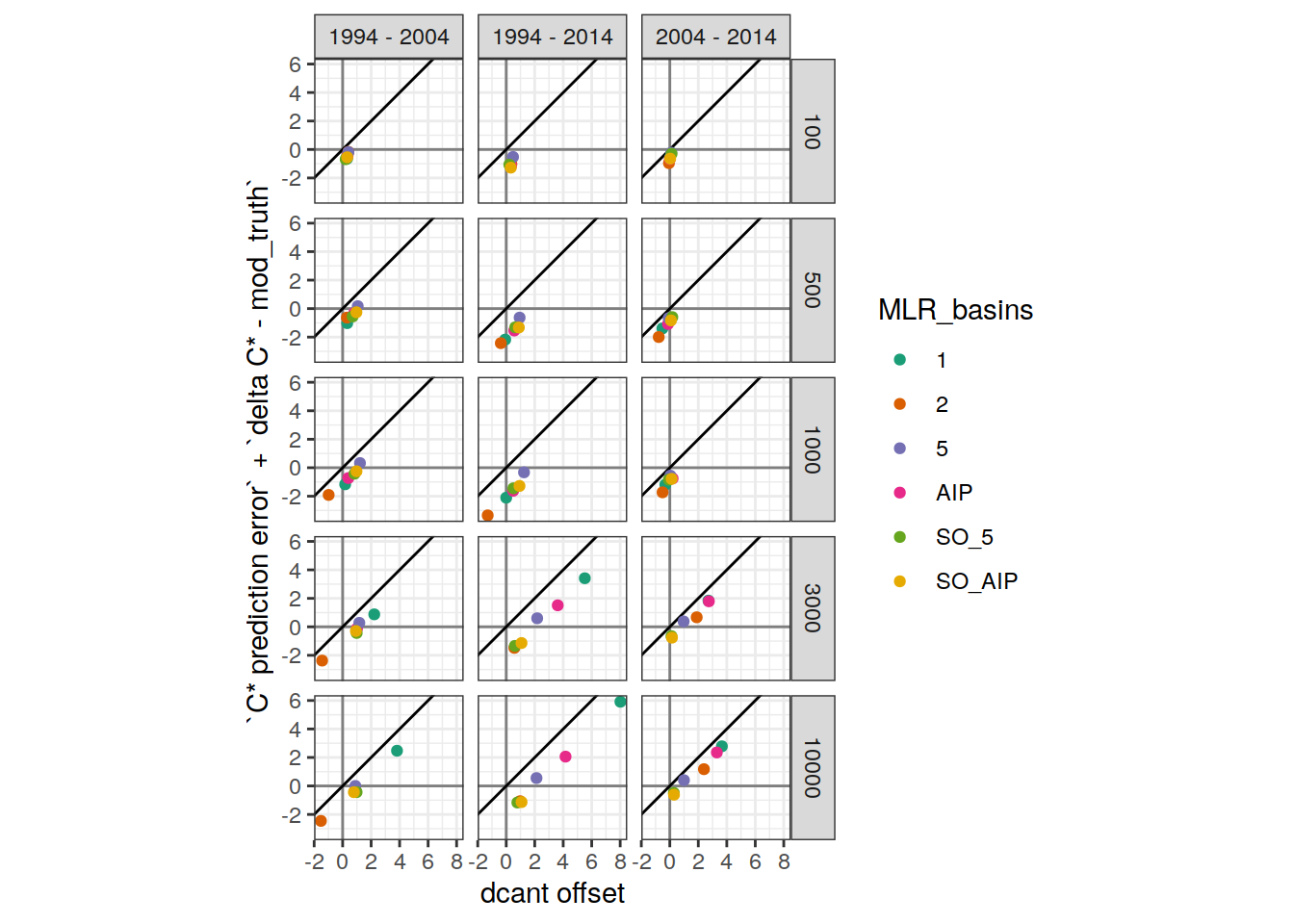

dcant_budget_global_bias_all_decomposition %>%
  ggplot(aes(`dcant offset`, `C* drift`, col = !!sym(config))) +
  geom_vline(xintercept = 0, col = "grey50") +
  geom_hline(yintercept = 0, col = "grey50") +
  geom_abline(intercept = 0, slope = 1) +
  geom_point() +
  coord_fixed() +
  scale_color_brewer(palette = "Dark2") +
  facet_grid(inv_depth ~ period)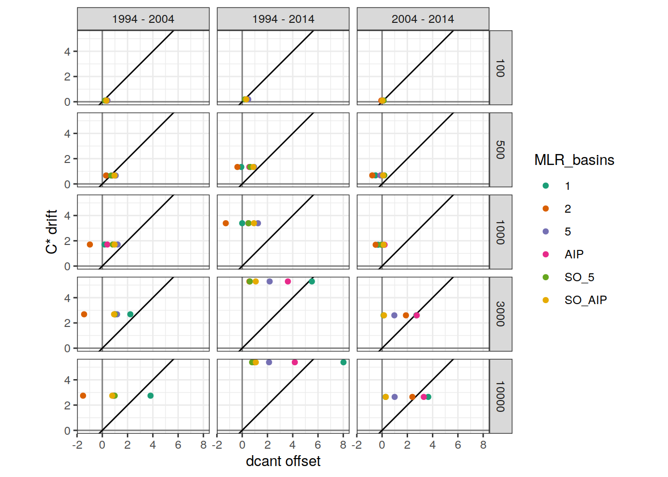

dcant_budget_global_bias_all_decomposition %>%
  ggplot(aes(
    `dcant offset` - `C* drift`,
    `C* prediction error`,
    col = !!sym(config)
  )) +
  geom_vline(xintercept = 0, col = "grey50") +
  geom_hline(yintercept = 0, col = "grey50") +
  geom_abline(intercept = 0, slope = 1) +
  geom_point() +
  coord_fixed() +
  scale_color_brewer(palette = "Dark2") +
  facet_grid(inv_depth ~ period)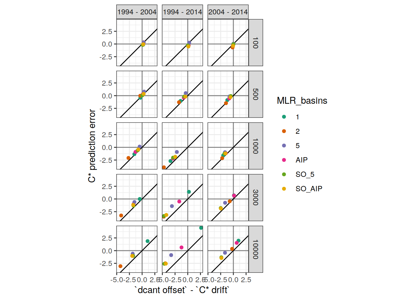

dcant_budget_global_bias_all_decomposition %>%
  ggplot(aes(
    x = period,
    fill = !!sym(config),
    col = !!sym(config)
  )) +
  geom_hline(yintercept = 0) +
  geom_point(
    aes(y = `dcant offset`, shape = "dcant offset"),
    position = position_nudge(x = -0.05),
    alpha = 0.5
  ) +
  geom_point(
    aes(y = `dcant offset` - `C* drift`, shape = "dcant offset - C* drift"),
    position = position_nudge(x = 0.05),
    alpha = 0.5
  ) +
  scale_color_brewer(palette = "Dark2") +
  scale_fill_brewer(palette = "Dark2") +
  scale_shape_manual(values = c(21,23)) +
  facet_grid(inv_depth ~ .)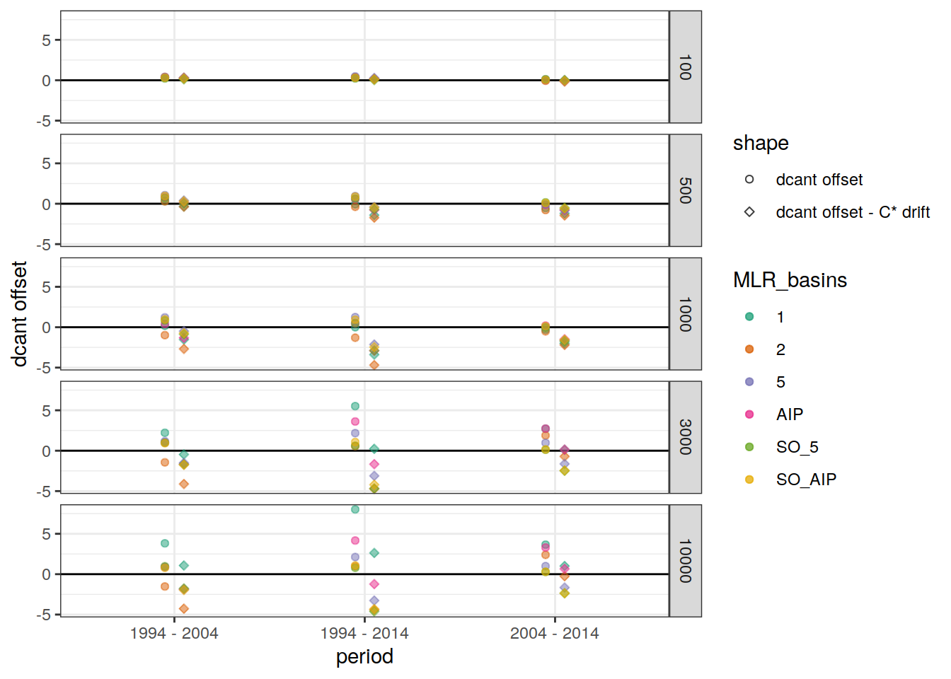

dcant_budget_global_bias_all_decomposition <-
  dcant_budget_global_bias_all_decomposition %>%
  mutate(
    `dcant offset rel` = 100 * `dcant offset` / mod_truth,
    `dcant offset rel corr` = 100 * (`dcant offset` - `C* drift`) / mod_truth,
    `C* prediction error rel` = 100 * (`C* prediction error`) / mod_truth
  )

dcant_budget_global_bias_all_decomposition %>%
  ggplot(aes(
    x = period,
    fill = !!sym(config),
    col = !!sym(config)
  )) +
  geom_hline(yintercept = 0) +
  geom_point(
    aes(y = `dcant offset rel`, shape = "dcant offset"),
    position = position_nudge(x = -0.05),
    alpha = 0.5
  ) +
  geom_point(
    aes(y = `dcant offset rel corr`, shape = "dcant offset - C* drift"),
    position = position_nudge(x = 0.05),
    alpha = 0.5
  ) +
  scale_color_brewer(palette = "Dark2") +
  scale_fill_brewer(palette = "Dark2") +
  scale_shape_manual(values = c(21,23)) +
  facet_grid(inv_depth ~ .)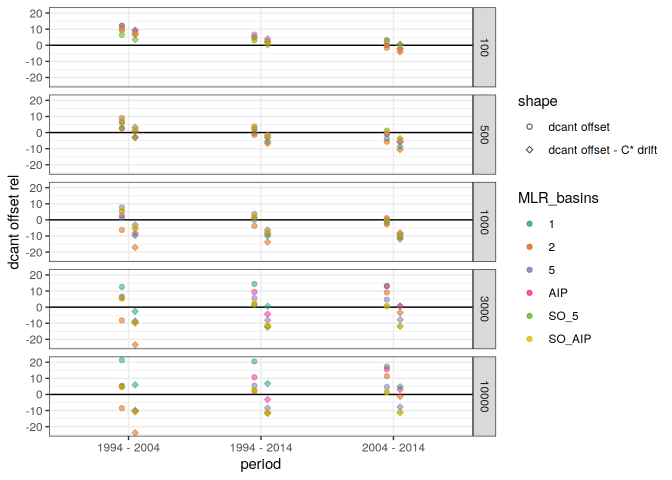

dcant_budget_global_bias_all_decomposition <-
  dcant_budget_global_bias_all_decomposition %>%
  pivot_longer(-c(inv_depth:period),
               names_to = "estimate",
               values_to = "value")


dcant_budget_global_bias_all_decomposition %>%
  group_by(inv_depth, estimate) %>%
  summarise(mean = mean(value),
            sd = sd(value)) %>%
  ungroup() %>%
  kable() %>%
  kable_styling() %>%
  scroll_box(height = "300px")

`summarise()` has grouped output by 'inv_depth'. You can override using the
`.groups` argument.

inv_depth	estimate	mean	sd
100	C* drift	0.1286667	0.0468113
100	C* prediction error	-0.1510556	0.2812768
100	C* prediction error rel	-2.9194349	6.8020742
100	dcant offset	0.2374444	0.1629793
100	dcant offset rel	5.2630346	4.1819014
100	dcant offset rel corr	2.5497943	4.0469449
100	delta C* - mod_truth	-0.5213333	0.2108844
100	mod_truth	4.7563333	1.7425592
500	C* drift	0.8940000	0.3252731
500	C* prediction error	-0.2760556	0.6051120
500	C* prediction error rel	-1.4564125	3.9388511
500	dcant offset	0.3040556	0.5528677
500	dcant offset rel	2.0181420	3.9211493
500	dcant offset rel corr	-3.2716308	3.6827364
500	delta C* - mod_truth	-0.7573333	0.2782179
500	mod_truth	16.9600000	6.2242462
1000	C* drift	2.2606667	0.8224770
1000	C* prediction error	-1.5105000	0.9391364
1000	C* prediction error rel	-6.5764080	3.4588655
1000	dcant offset	0.2196111	0.7040770
1000	dcant offset rel	1.0692998	3.4684847
1000	dcant offset rel corr	-8.9125027	3.2525472
1000	delta C* - mod_truth	0.3930000	0.1726274
1000	mod_truth	22.7516667	8.3557301
3000	C* drift	3.5240000	1.2825060
3000	C* prediction error	-1.1812222	1.4483787
3000	C* prediction error rel	-4.7454844	5.5474568
3000	dcant offset	1.5006111	1.5374143
3000	dcant offset rel	5.7814635	5.6625770
3000	dcant offset rel corr	-8.0350395	5.9629918
3000	delta C* - mod_truth	1.3360000	0.4970814
3000	mod_truth	25.6453333	9.4254881
10000	C* drift	3.5926667	1.3076595
10000	C* prediction error	-0.4142222	1.9411466
10000	C* prediction error rel	-1.7720957	7.4422688
10000	dcant offset	1.8828333	2.1175031
10000	dcant offset rel	7.1142306	7.6395068
10000	dcant offset rel corr	-6.7598057	7.9334250
10000	delta C* - mod_truth	0.9513333	0.3587727
10000	mod_truth	26.0420000	9.5725748

dcant_budget_global_bias_all_decomposition %>%
  group_by(inv_depth, estimate, period) %>%
  summarise(mean = mean(value),
            sd = sd(value)) %>%
  ungroup() %>%
  kable() %>%
  kable_styling() %>%
  scroll_box(height = "300px")

`summarise()` has grouped output by 'inv_depth', 'estimate'. You can override
using the `.groups` argument.

inv_depth	estimate	period	mean	sd
100	C* drift	1994 - 2004	0.0960000	0.0000000
100	C* drift	1994 - 2014	0.1930000	0.0000000
100	C* drift	2004 - 2014	0.0970000	0.0000000
100	C* prediction error	1994 - 2004	0.0608333	0.2236725
100	C* prediction error	1994 - 2014	-0.2361667	0.2569696
100	C* prediction error	2004 - 2014	-0.2778333	0.2666041
100	C* prediction error rel	1994 - 2004	1.8328814	6.7391520
100	C* prediction error rel	1994 - 2014	-3.3104383	3.6020407
100	C* prediction error rel	2004 - 2014	-7.2807477	6.9864816
100	dcant offset	1994 - 2004	0.3335000	0.0715395
100	dcant offset	1994 - 2014	0.3435000	0.0838493
100	dcant offset	2004 - 2014	0.0353333	0.0676392
100	dcant offset rel	1994 - 2004	10.0482073	2.1554534
100	dcant offset rel	1994 - 2014	4.8149706	1.1753472
100	dcant offset rel	2004 - 2014	0.9259259	1.7725167
100	dcant offset rel corr	1994 - 2004	7.1557698	2.1554534
100	dcant offset rel corr	1994 - 2014	2.1096159	1.1753472
100	dcant offset rel corr	2004 - 2014	-1.6160028	1.7725167
100	delta C* - mod_truth	1994 - 2004	-0.5030000	0.0000000
100	delta C* - mod_truth	1994 - 2014	-0.7810000	0.0000000
100	delta C* - mod_truth	2004 - 2014	-0.2800000	0.0000000
100	mod_truth	1994 - 2004	3.3190000	0.0000000
100	mod_truth	1994 - 2014	7.1340000	0.0000000
100	mod_truth	2004 - 2014	3.8160000	0.0000000
500	C* drift	1994 - 2004	0.6650000	0.0000000
500	C* drift	1994 - 2014	1.3410000	0.0000000
500	C* drift	2004 - 2014	0.6760000	0.0000000
500	C* prediction error	1994 - 2004	0.1786667	0.4020839
500	C* prediction error	1994 - 2014	-0.4335000	0.6483066
500	C* prediction error	2004 - 2014	-0.5733333	0.5282525
500	C* prediction error rel	1994 - 2004	1.5212147	3.4234475
500	C* prediction error rel	1994 - 2014	-1.7040094	2.5483752
500	C* prediction error rel	2004 - 2014	-4.1864427	3.8572652
500	dcant offset	1994 - 2004	0.6920000	0.3209654
500	dcant offset	1994 - 2014	0.4286667	0.5355661
500	dcant offset	2004 - 2014	-0.2085000	0.3673046
500	dcant offset rel	1994 - 2004	5.8918689	2.7327835
500	dcant offset rel	1994 - 2014	1.6850105	2.1052127
500	dcant offset rel	2004 - 2014	-1.5224535	2.6820346
500	dcant offset rel corr	1994 - 2004	0.2298851	2.7327835
500	dcant offset rel corr	1994 - 2014	-3.5862159	2.1052127
500	dcant offset rel corr	2004 - 2014	-6.4585615	2.6820346
500	delta C* - mod_truth	1994 - 2004	-0.6140000	0.0000000
500	delta C* - mod_truth	1994 - 2014	-1.1360000	0.0000000
500	delta C* - mod_truth	2004 - 2014	-0.5220000	0.0000000
500	mod_truth	1994 - 2004	11.7450000	0.0000000
500	mod_truth	1994 - 2014	25.4400000	0.0000000
500	mod_truth	2004 - 2014	13.6950000	0.0000000
1000	C* drift	1994 - 2004	1.7050000	0.0000000
1000	C* drift	1994 - 2014	3.3910000	0.0000000
1000	C* drift	2004 - 2014	1.6860000	0.0000000
1000	C* prediction error	1994 - 2004	-0.8715000	0.7770932
1000	C* prediction error	1994 - 2014	-2.2765000	1.0015144
1000	C* prediction error	2004 - 2014	-1.3835000	0.4223386
1000	C* prediction error rel	1994 - 2004	-5.5509554	4.9496385
1000	C* prediction error rel	1994 - 2014	-6.6706713	2.9346687
1000	C* prediction error rel	2004 - 2014	-7.5075971	2.2918310
1000	dcant offset	1994 - 2004	0.4351667	0.7915171
1000	dcant offset	1994 - 2014	0.3115000	0.8971898
1000	dcant offset	2004 - 2014	-0.0878333	0.2733097
1000	dcant offset rel	1994 - 2004	2.7717622	5.0415104
1000	dcant offset rel	1994 - 2014	0.9127670	2.6289735
1000	dcant offset rel	2004 - 2014	-0.4766298	1.4831216
1000	dcant offset rel corr	1994 - 2004	-8.0881104	5.0415104
1000	dcant offset rel corr	1994 - 2014	-9.0236470	2.6289735
1000	dcant offset rel corr	2004 - 2014	-9.6257507	1.4831216
1000	delta C* - mod_truth	1994 - 2004	0.1800000	0.0000000
1000	delta C* - mod_truth	1994 - 2014	0.5900000	0.0000000
1000	delta C* - mod_truth	2004 - 2014	0.4090000	0.0000000
1000	mod_truth	1994 - 2004	15.7000000	0.0000000
1000	mod_truth	1994 - 2014	34.1270000	0.0000000
1000	mod_truth	2004 - 2014	18.4280000	0.0000000
3000	C* drift	1994 - 2004	2.6840000	0.0000000
3000	C* drift	1994 - 2014	5.2860000	0.0000000
3000	C* drift	2004 - 2014	2.6020000	0.0000000
3000	C* prediction error	1994 - 2004	-1.2195000	1.1000356
3000	C* prediction error	1994 - 2014	-1.7421667	1.9563941
3000	C* prediction error	2004 - 2014	-0.5820000	1.1334627
3000	C* prediction error rel	1994 - 2004	-6.9132653	6.2360294
3000	C* prediction error rel	1994 - 2014	-4.5288725	5.0857702
3000	C* prediction error rel	2004 - 2014	-2.7943153	5.4420139
3000	dcant offset	1994 - 2004	0.8121667	1.2055340
3000	dcant offset	1994 - 2014	2.2595000	1.9716848
3000	dcant offset	2004 - 2014	1.4301667	1.1957154
3000	dcant offset rel	1994 - 2004	4.6041194	6.8340928
3000	dcant offset rel	1994 - 2014	5.8737132	5.1255195
3000	dcant offset rel	2004 - 2014	6.8665578	5.7409037
3000	dcant offset rel corr	1994 - 2004	-10.6113001	6.8340928
3000	dcant offset rel corr	1994 - 2014	-7.8675782	5.1255195
3000	dcant offset rel corr	2004 - 2014	-5.6262403	5.7409037
3000	delta C* - mod_truth	1994 - 2004	0.8780000	0.0000000
3000	delta C* - mod_truth	1994 - 2014	2.0040000	0.0000000
3000	delta C* - mod_truth	2004 - 2014	1.1260000	0.0000000
3000	mod_truth	1994 - 2004	17.6400000	0.0000000
3000	mod_truth	1994 - 2014	38.4680000	0.0000000
3000	mod_truth	2004 - 2014	20.8280000	0.0000000
10000	C* drift	1994 - 2004	2.7430000	0.0000000
10000	C* drift	1994 - 2014	5.3890000	0.0000000
10000	C* drift	2004 - 2014	2.6460000	0.0000000
10000	C* prediction error	1994 - 2004	-0.7830000	1.5735600
10000	C* prediction error	1994 - 2014	-0.5678333	2.7881877
10000	C* prediction error	2004 - 2014	0.1081667	1.4290933
10000	C* prediction error rel	1994 - 2004	-4.3738130	8.7898561
10000	C* prediction error rel	1994 - 2014	-1.4536347	7.1376691
10000	C* prediction error rel	2004 - 2014	0.5111605	6.7534301
10000	dcant offset	1994 - 2004	0.9718333	1.6954329
10000	dcant offset	1994 - 2014	2.8565000	2.8245136
10000	dcant offset	2004 - 2014	1.8201667	1.5014549
10000	dcant offset rel	1994 - 2004	5.4286299	9.4706338
10000	dcant offset rel	1994 - 2014	7.3125464	7.2306623
10000	dcant offset rel	2004 - 2014	8.6015154	7.0953875
10000	dcant offset rel corr	1994 - 2004	-9.8936804	9.4706338
10000	dcant offset rel corr	1994 - 2014	-6.4831170	7.2306623
10000	dcant offset rel corr	2004 - 2014	-3.9026196	7.0953875
10000	delta C* - mod_truth	1994 - 2004	0.6010000	0.0000000
10000	delta C* - mod_truth	1994 - 2014	1.4270000	0.0000000
10000	delta C* - mod_truth	2004 - 2014	0.8260000	0.0000000
10000	mod_truth	1994 - 2004	17.9020000	0.0000000
10000	mod_truth	1994 - 2014	39.0630000	0.0000000
10000	mod_truth	2004 - 2014	21.1610000	0.0000000

Session information

sessionInfo()

R version 4.1.2 (2021-11-01)
Platform: x86_64-pc-linux-gnu (64-bit)
Running under: openSUSE Leap 15.3

Matrix products: default
BLAS:   /usr/local/R-4.1.2/lib64/R/lib/libRblas.so
LAPACK: /usr/local/R-4.1.2/lib64/R/lib/libRlapack.so

locale:
 [1] LC_CTYPE=en_US.UTF-8       LC_NUMERIC=C              
 [3] LC_TIME=en_US.UTF-8        LC_COLLATE=en_US.UTF-8    
 [5] LC_MONETARY=en_US.UTF-8    LC_MESSAGES=en_US.UTF-8   
 [7] LC_PAPER=en_US.UTF-8       LC_NAME=C                 
 [9] LC_ADDRESS=C               LC_TELEPHONE=C            
[11] LC_MEASUREMENT=en_US.UTF-8 LC_IDENTIFICATION=C       

attached base packages:
[1] stats     graphics  grDevices utils     datasets  methods   base     

other attached packages:
 [1] kableExtra_1.3.4   geomtextpath_0.1.0 colorspace_2.0-2   marelac_2.1.10    
 [5] shape_1.4.6        ggforce_0.3.3      metR_0.11.0        scico_1.3.0       
 [9] patchwork_1.1.1    collapse_1.7.0     forcats_0.5.1      stringr_1.4.0     
[13] dplyr_1.0.7        purrr_0.3.4        readr_2.1.1        tidyr_1.1.4       
[17] tibble_3.1.6       ggplot2_3.3.5      tidyverse_1.3.1    workflowr_1.7.0   

loaded via a namespace (and not attached):
 [1] fs_1.5.2           gghalves_0.1.1     bit64_4.0.5        lubridate_1.8.0   
 [5] gsw_1.0-6          RColorBrewer_1.1-2 webshot_0.5.2      httr_1.4.2        
 [9] rprojroot_2.0.2    tools_4.1.2        backports_1.4.1    bslib_0.3.1       
[13] utf8_1.2.2         R6_2.5.1           DBI_1.1.2          withr_2.4.3       
[17] tidyselect_1.1.1   processx_3.5.2     bit_4.0.4          compiler_4.1.2    
[21] git2r_0.29.0       textshaping_0.3.6  cli_3.1.1          rvest_1.0.2       
[25] xml2_1.3.3         labeling_0.4.2     sass_0.4.0         scales_1.1.1      
[29] checkmate_2.0.0    SolveSAPHE_2.1.0   callr_3.7.0        systemfonts_1.0.3 
[33] digest_0.6.29      svglite_2.0.0      rmarkdown_2.11     oce_1.5-0         
[37] pkgconfig_2.0.3    htmltools_0.5.2    highr_0.9          dbplyr_2.1.1      
[41] fastmap_1.1.0      rlang_1.0.2        readxl_1.3.1       rstudioapi_0.13   
[45] jquerylib_0.1.4    generics_0.1.1     farver_2.1.0       jsonlite_1.7.3    
[49] vroom_1.5.7        magrittr_2.0.1     Rcpp_1.0.8         munsell_0.5.0     
[53] fansi_1.0.2        lifecycle_1.0.1    stringi_1.7.6      whisker_0.4       
[57] yaml_2.2.1         MASS_7.3-55        grid_4.1.2         parallel_4.1.2    
[61] promises_1.2.0.1   crayon_1.4.2       haven_2.4.3        hms_1.1.1         
[65] seacarb_3.3.0      knitr_1.37         ps_1.6.0           pillar_1.6.4      
[69] reprex_2.0.1       glue_1.6.0         evaluate_0.14      getPass_0.2-2     
[73] data.table_1.14.2  modelr_0.1.8       vctrs_0.3.8        tzdb_0.2.0        
[77] tweenr_1.0.2       httpuv_1.6.5       cellranger_1.1.0   gtable_0.3.0      
[81] polyclip_1.10-0    assertthat_0.2.1   xfun_0.29          broom_0.7.11      
[85] later_1.3.0        viridisLite_0.4.0  ellipsis_0.3.2     here_1.0.1