eMLR - model fitting
Jens Daniel Müller
20 March, 2021
Last updated: 2021-03-20
Checks: 7 0
Knit directory: emlr_obs_v_XXX/
This reproducible R Markdown analysis was created with workflowr (version 1.6.2). The Checks tab describes the reproducibility checks that were applied when the results were created. The Past versions tab lists the development history.
Great! Since the R Markdown file has been committed to the Git repository, you know the exact version of the code that produced these results.
Great job! The global environment was empty. Objects defined in the global environment can affect the analysis in your R Markdown file in unknown ways. For reproduciblity it’s best to always run the code in an empty environment.
The command set.seed(20200707) was run prior to running the code in the R Markdown file. Setting a seed ensures that any results that rely on randomness, e.g. subsampling or permutations, are reproducible.
Great job! Recording the operating system, R version, and package versions is critical for reproducibility.
Nice! There were no cached chunks for this analysis, so you can be confident that you successfully produced the results during this run.
Great job! Using relative paths to the files within your workflowr project makes it easier to run your code on other machines.
Great! You are using Git for version control. Tracking code development and connecting the code version to the results is critical for reproducibility.
The results in this page were generated with repository version 2b99ba0. See the Past versions tab to see a history of the changes made to the R Markdown and HTML files.
Note that you need to be careful to ensure that all relevant files for the analysis have been committed to Git prior to generating the results (you can use wflow_publish or wflow_git_commit). workflowr only checks the R Markdown file, but you know if there are other scripts or data files that it depends on. Below is the status of the Git repository when the results were generated:
Ignored files:
    Ignored:    .Rhistory
    Ignored:    .Rproj.user/
Note that any generated files, e.g. HTML, png, CSS, etc., are not included in this status report because it is ok for generated content to have uncommitted changes.
These are the previous versions of the repository in which changes were made to the R Markdown (analysis/eMLR_model_fitting.Rmd) and HTML (docs/eMLR_model_fitting.html) files. If you’ve configured a remote Git repository (see ?wflow_git_remote), click on the hyperlinks in the table below to view the files as they were in that past version.
| File | Version | Author | Date | Message |
|---|---|---|---|---|
| Rmd | 2b99ba0 | jens-daniel-mueller | 2021-03-20 | included vif removel option |
| html | 330dcd0 | jens-daniel-mueller | 2021-03-20 | Build site. |
| Rmd | 4df8990 | jens-daniel-mueller | 2021-03-20 | added vif calculation and plots |
| html | 83a13de | jens-daniel-mueller | 2021-03-20 | Build site. |
| html | cf98c6d | jens-daniel-mueller | 2021-03-16 | Build site. |
| html | a1d52ff | jens-daniel-mueller | 2021-03-15 | Build site. |
| html | 0bade3b | jens-daniel-mueller | 2021-03-15 | Build site. |
| html | 27c1f4b | jens-daniel-mueller | 2021-03-14 | Build site. |
| html | af75ebf | jens-daniel-mueller | 2021-03-14 | Build site. |
| html | 5017709 | jens-daniel-mueller | 2021-03-11 | Build site. |
| html | 585b07f | jens-daniel-mueller | 2021-03-11 | Build site. |
| html | 6482ed7 | jens-daniel-mueller | 2021-03-11 | Build site. |
| html | 85a5ed2 | jens-daniel-mueller | 2021-03-10 | Build site. |
| html | 00688a1 | jens-daniel-mueller | 2021-03-05 | Build site. |
| html | 6c0bec6 | jens-daniel-mueller | 2021-03-05 | Build site. |
| html | 3c2ec33 | jens-daniel-mueller | 2021-03-05 | Build site. |
| html | af70b94 | jens-daniel-mueller | 2021-03-04 | Build site. |
| Rmd | c9cf1fd | jens-daniel-mueller | 2021-03-04 | rebuild with NA in Cant replaced by 0 |
| html | 27ae473 | jens-daniel-mueller | 2021-02-24 | Build site. |
| Rmd | 7f77d91 | jens-daniel-mueller | 2021-02-24 | removed log10 color scale |
| html | fec3558 | jens-daniel-mueller | 2021-02-24 | Build site. |
| Rmd | 9ebedac | jens-daniel-mueller | 2021-02-24 | latitudinal residual plots |
| html | 4bc00ea | jens-daniel-mueller | 2021-02-24 | Build site. |
| Rmd | de11bfe | jens-daniel-mueller | 2021-02-24 | clean up purrr approach and residual plots |
| html | 42eca5d | jens-daniel-mueller | 2021-02-24 | Build site. |
| Rmd | 06a2f3b | jens-daniel-mueller | 2021-02-24 | purrr residual plots by basin |
| html | a1ba577 | jens-daniel-mueller | 2021-02-24 | Build site. |
| Rmd | 9ae7d87 | jens-daniel-mueller | 2021-02-24 | loop residual plots by basin |
| html | 071743d | jens-daniel-mueller | 2021-02-24 | Build site. |
| Rmd | c45672c | jens-daniel-mueller | 2021-02-24 | added residual plots |
| html | ac1a836 | jens-daniel-mueller | 2021-02-24 | Build site. |
| Rmd | 5f655e0 | jens-daniel-mueller | 2021-02-24 | added plots back to after switching to map aproach |
| html | b03fbd3 | jens-daniel-mueller | 2021-02-24 | Build site. |
| Rmd | c69736b | jens-daniel-mueller | 2021-02-24 | added plots back to after switching to map aproach |
| html | 86406d5 | jens-daniel-mueller | 2021-02-24 | Build site. |
| Rmd | 1b3c171 | jens-daniel-mueller | 2021-02-24 | introduced purrr::map to model fitting, rebuild all |
| html | 3d3b4cc | jens-daniel-mueller | 2021-02-23 | Build site. |
| Rmd | cbfc388 | jens-daniel-mueller | 2021-02-23 | introduced purrr::map to model fitting |
| html | 7b672f7 | jens-daniel-mueller | 2021-01-11 | Build site. |
| html | 33ba23c | jens-daniel-mueller | 2021-01-07 | Build site. |
| Rmd | 0ad30ba | jens-daniel-mueller | 2021-01-07 | removed GLODAP gamma filter, target variable mapped by eras+era |
| html | 318609d | jens-daniel-mueller | 2020-12-23 | adapted more variable predictor selection |
| html | 9d0b2d0 | jens-daniel-mueller | 2020-12-23 | Build site. |
| html | 0aa2b50 | jens-daniel-mueller | 2020-12-23 | remove html before duplication |
| html | 39113c3 | jens-daniel-mueller | 2020-12-23 | Build site. |
| Rmd | bef9220 | jens-daniel-mueller | 2020-12-23 | rebuild before sensitivity test |
| html | 2886da0 | jens-daniel-mueller | 2020-12-19 | Build site. |
| html | 02f0ee9 | jens-daniel-mueller | 2020-12-18 | cleaned up for copying template |
| html | 965dba3 | jens-daniel-mueller | 2020-12-18 | Build site. |
| html | 5d452fe | jens-daniel-mueller | 2020-12-18 | Build site. |
| Rmd | ca65bf5 | jens-daniel-mueller | 2020-12-18 | rebuild after final cleaning |
| html | 7bcb4eb | jens-daniel-mueller | 2020-12-18 | Build site. |
| html | d397028 | jens-daniel-mueller | 2020-12-18 | Build site. |
| Rmd | 7e1b1c0 | jens-daniel-mueller | 2020-12-18 | rebuild without na predictors |
| html | 7131186 | jens-daniel-mueller | 2020-12-17 | Build site. |
| Rmd | 737d904 | jens-daniel-mueller | 2020-12-17 | rebuild without na predictors |
| html | 22b07fb | jens-daniel-mueller | 2020-12-17 | Build site. |
| html | a84ff3c | jens-daniel-mueller | 2020-12-17 | Build site. |
| Rmd | 40369db | jens-daniel-mueller | 2020-12-17 | model selection criterion added |
| html | 5b48ef5 | jens-daniel-mueller | 2020-12-17 | Build site. |
| Rmd | e6ed2bc | jens-daniel-mueller | 2020-12-17 | plotted model results |
| html | f3a708f | jens-daniel-mueller | 2020-12-17 | Build site. |
| Rmd | 7c8ace9 | jens-daniel-mueller | 2020-12-17 | new MLR fitting routine, rmse corrected |
| html | e4ca289 | jens-daniel-mueller | 2020-12-16 | Build site. |
| Rmd | 3d5a3e2 | jens-daniel-mueller | 2020-12-16 | new MLR fitting routine |
| html | 158fe26 | jens-daniel-mueller | 2020-12-15 | Build site. |
| html | 7a9a4cb | jens-daniel-mueller | 2020-12-15 | Build site. |
| html | 61b263c | jens-daniel-mueller | 2020-12-15 | Build site. |
| html | 4d612dd | jens-daniel-mueller | 2020-12-15 | Build site. |
| html | e91cebd | jens-daniel-mueller | 2020-12-15 | Build site. |
| Rmd | d7992c4 | jens-daniel-mueller | 2020-12-15 | eMLR target variable selection |
| html | 953caf3 | jens-daniel-mueller | 2020-12-15 | Build site. |
| html | 42daf5c | jens-daniel-mueller | 2020-12-14 | Build site. |
| Rmd | 923aa7f | jens-daniel-mueller | 2020-12-14 | rebuild with new path and auto folder creation |
| html | 984697e | jens-daniel-mueller | 2020-12-12 | Build site. |
| html | 3ebff89 | jens-daniel-mueller | 2020-12-12 | Build site. |
| html | ba112d3 | jens-daniel-mueller | 2020-12-11 | Build site. |
| Rmd | 91b2b29 | jens-daniel-mueller | 2020-12-11 | selectable basinmask, try 5 |
| html | b01a367 | jens-daniel-mueller | 2020-12-09 | Build site. |
| Rmd | 71c63b0 | jens-daniel-mueller | 2020-12-09 | rerun with variable predictor assignment |
| html | 24a632f | jens-daniel-mueller | 2020-12-07 | Build site. |
| html | 92dca91 | jens-daniel-mueller | 2020-12-07 | Build site. |
| html | 6a8004b | jens-daniel-mueller | 2020-12-07 | Build site. |
| html | 70bf1a5 | jens-daniel-mueller | 2020-12-07 | Build site. |
| html | 7555355 | jens-daniel-mueller | 2020-12-07 | Build site. |
| html | 143d6fa | jens-daniel-mueller | 2020-12-07 | Build site. |
| html | abc6818 | jens-daniel-mueller | 2020-12-03 | Build site. |
| Rmd | 992ba15 | jens-daniel-mueller | 2020-12-03 | rebuild with variable inventory depth |
| html | c8c2e7b | jens-daniel-mueller | 2020-12-03 | Build site. |
| Rmd | 83203db | jens-daniel-mueller | 2020-12-03 | calculate cant with variable inventory depth |
| html | 090e4d5 | jens-daniel-mueller | 2020-12-02 | Build site. |
| html | 7c25f7a | jens-daniel-mueller | 2020-12-02 | Build site. |
| html | ec8dc38 | jens-daniel-mueller | 2020-12-02 | Build site. |
| html | c987de1 | jens-daniel-mueller | 2020-12-02 | Build site. |
| html | f8358f8 | jens-daniel-mueller | 2020-12-02 | Build site. |
| html | b03ddb8 | jens-daniel-mueller | 2020-12-02 | Build site. |
| Rmd | 9183e8f | jens-daniel-mueller | 2020-12-02 | revised assignment of era to eras |
| html | 22d0127 | jens-daniel-mueller | 2020-12-01 | Build site. |
| html | 0ff728b | jens-daniel-mueller | 2020-12-01 | Build site. |
| html | 91435ae | jens-daniel-mueller | 2020-12-01 | Build site. |
| Rmd | 17d09be | jens-daniel-mueller | 2020-12-01 | auto eras naming |
| html | cf19652 | jens-daniel-mueller | 2020-11-30 | Build site. |
| Rmd | 0895ad6 | jens-daniel-mueller | 2020-11-30 | rebuild with all plot output |
| Rmd | 2842970 | jens-daniel-mueller | 2020-11-30 | cleaned for eMLR part only |
| html | 196be51 | jens-daniel-mueller | 2020-11-30 | Build site. |
| Rmd | 7a4b015 | jens-daniel-mueller | 2020-11-30 | first rebuild on ETH server |
| Rmd | bc61ce3 | Jens Müller | 2020-11-30 | Initial commit |
1 Required data
Required are:
- cleaned and prepared GLODAPv2_2020 file
GLODAP <-
  read_csv(paste(path_version_data,
                 "GLODAPv2.2020_MLR_fitting_ready.csv",
                 sep = ""))
2 Predictor combinations
Find all possible combinations of following considered predictor variables:
- sal, temp, aou, nitrate, silicate, phosphate, phosphate_star
# the following code is a workaround to find all predictor combinations
# using the olsrr package and fit all models for one era, slab, and basin

i_basin <- unique(GLODAP$basin)[1]
i_era   <- unique(GLODAP$era)[1]

# subset one basin and era for fitting
GLODAP_basin_era <- GLODAP %>%
  filter(basin == i_basin, era == i_era)

i_gamma_slab <- unique(GLODAP_basin_era$gamma_slab)[1]
print(i_gamma_slab)

# subset one gamma slab
GLODAP_basin_era_slab <- GLODAP_basin_era %>%
  filter(gamma_slab == i_gamma_slab)

# fit the full linear model, i.e. all predictor combinations
lm_full <- lm(paste(
  params_local$MLR_target,
  paste(params_local$MLR_predictors, collapse = " + "),
  sep = " ~ "
),
data = GLODAP_basin_era_slab)

# fit linear models for all possible predictor combinations
# unfortunately, this functions does not provide model coefficients (yet)
lm_all <- ols_step_all_possible(lm_full)

# convert to tibble
lm_all <- as_tibble(lm_all)

# format model formula
lm_all <- lm_all %>%
  select(n, predictors) %>%
  mutate(model = str_replace_all(predictors, " ", " + "),
         model = paste(params_local$MLR_target, "~", model))

# remove helper objects
rm(i_gamma_slab,
   i_era,
   i_basin,
   GLODAP_basin_era,
   GLODAP_basin_era_slab,
   lm_full)
3 Apply predictor threshold
Select combinations with a total number of predictors in the range:
- Minimum: 2
- Maximum: 5
lm_all <- lm_all %>%
  filter(n >= params_local$MLR_predictors_min,
         n <= params_local$MLR_predictors_max)
This results in a total number of MLR models of:
- 112
4 Fit all models
Individual linear regression models were fitted for the chosen target variable:
- cstar_tref
as a function of each predictor combination. Fitting was performed separately within each basin, era, and slab. Model diagnostics, such as the root mean squared error (RMSE), were calculated for each fitted model.
# prepare nested data frame

GLODAP %>%
  # filter(basin %in% unique(GLODAP$basin)[1],
  #        era %in% unique(GLODAP$era)[c(1,2)],
  #        gamma_slab %in% unique(GLODAP$gamma_slab)[c(5,6)]) %>%
  filter_all(any_vars(is.na(.)))

GLODAP_nested <- GLODAP %>%
  filter(basin %in% unique(GLODAP$basin)[1],
         era %in% unique(GLODAP$era)[c(1,2)],
         gamma_slab %in% unique(GLODAP$gamma_slab)[c(5,6)]) %>%
  group_by(gamma_slab, era, basin) %>%
  nest()

# expand with model definitions

GLODAP_nested_lm <- expand_grid(
  GLODAP_nested,
  lm_all
)

# fit models and extract tidy model output

GLODAP_nested_lm_fit <- GLODAP_nested_lm %>%
  mutate(
    fit = map2(.x = data, .y = model,
               ~ lm(as.formula(.y), data = .x)),
    tidied = map(fit, tidy),
    glanced = map(fit, glance),
    augmented = map(fit, augment),
    vif = map(fit, ols_vif_tol)
  )

# print(object.size(GLODAP_nested), units = "MB")
# print(object.size(GLODAP_nested_lm), units = "MB")
# print(object.size(GLODAP_nested_lm_fit), units = "MB")
5 Tidy models
# extract glanced model output (model diagnostics, such as AIC)
GLODAP_glanced <- GLODAP_nested_lm_fit %>%
  select(-c(data, fit, tidied, augmented, vif)) %>%
  unnest(glanced) %>%
  rename(n_predictors = n)

# extract tidy model output (model coefficients)
GLODAP_tidy <- GLODAP_nested_lm_fit %>%
  select(-c(data, fit, glanced, augmented, vif)) %>%
  unnest(tidied)

# extract augmented model output (fitted values and residuals)
GLODAP_augmented <- GLODAP_nested_lm_fit %>%
  select(-c(data, fit, tidied, glanced, vif)) %>%
  unnest(augmented)

# print(object.size(GLODAP_augmented), units = "MB")

# extract VIC from output
GLODAP_glanced_vif <- GLODAP_nested_lm_fit %>%
  select(-c(data, fit, tidied, augmented, glanced)) %>%
  unnest(vif)

# calculte max vif per model
GLODAP_glanced_vif_max <- GLODAP_glanced_vif %>%
  group_by(era, basin, gamma_slab, model, n) %>%
  summarise(vif_max = max(VIF)) %>%
  ungroup()

# calculate RMSE from augmented output
GLODAP_glanced_rmse <- GLODAP_augmented %>%
  group_by(gamma_slab, era, basin, model) %>%
  summarise(rmse = sqrt(c(crossprod(.resid)) / length(.resid))) %>%
  ungroup()

# add RMSE and vif_max to glanced output
GLODAP_glanced <- full_join(GLODAP_glanced, GLODAP_glanced_rmse)
GLODAP_glanced <- full_join(GLODAP_glanced, GLODAP_glanced_vif_max)
rm(GLODAP_glanced_rmse)
rm(GLODAP_glanced_vif_max)


# extract input data
GLODAP_data <- GLODAP_nested_lm_fit %>%
  select(-c(fit, tidied, glanced, augmented, vif)) %>%
  unnest(data)

# append input data with augmented data
GLODAP_augmented <- bind_cols(
  GLODAP_data,
  GLODAP_augmented %>% select(.fitted, .resid)
)

rm(GLODAP, GLODAP_nested, GLODAP_nested_lm, GLODAP_nested_lm_fit, lm_all,
   GLODAP_data)
6 Prepare coeffcients
Coefficients are prepared for the mapping of Cant and the chosen target variable.
6.1 VIF threshold
To avoid multicollinearity among predictors, models were excluded with a VIF above:
- 10
GLODAP_glanced_clean <- GLODAP_glanced %>%
  filter(vif_max <= params_local$vif_max)
6.2 Predictor selection
Within each basin and slab, the following number of best linear regression models was selected:
- 10
The criterion used to select the best models was:
- rmse
The criterion was summed up for two adjacent eras, and the models with lowest summed values were selected.
# calculate RMSE sum for adjacent eras
lm_all_eras <- GLODAP_glanced_clean  %>%
  select(basin, gamma_slab, model, era, AIC, BIC, rmse) %>%
  arrange(era) %>%
  group_by(basin, gamma_slab, model) %>%
  mutate(eras = paste(lag(era), era, sep = " --> "),
         rmse_sum = rmse + lag(rmse),
         aic_sum = AIC + lag(AIC),
         bic_sum = BIC + lag(BIC)
         ) %>%
  ungroup() %>%
  select(-c(era)) %>%
  drop_na()

# subset models with lowest summed criterion
# chose which criterion is applied

if (params_local$MLR_criterion == "aic") {
  lm_best_eras <- lm_all_eras %>%
    group_by(basin, gamma_slab, eras) %>%
    slice_min(order_by = aic_sum,
              with_ties = FALSE,
              n = params_local$MLR_number) %>%
    ungroup() %>%
    arrange(basin, gamma_slab, eras, model)
}

if (params_local$MLR_criterion == "bic") {
  lm_best_eras <- lm_all_eras %>%
    group_by(basin, gamma_slab, eras) %>%
    slice_min(order_by = bic_sum,
              with_ties = FALSE,
              n = params_local$MLR_number) %>%
    ungroup() %>%
    arrange(basin, gamma_slab, eras, model)
}

if (params_local$MLR_criterion == "rmse") {
  lm_best_eras <- lm_all_eras %>%
    group_by(basin, gamma_slab, eras) %>%
    slice_min(order_by = rmse_sum,
              with_ties = FALSE,
              n = params_local$MLR_number) %>%
    ungroup() %>%
    arrange(basin, gamma_slab, eras, model)
}


# print table
lm_best_eras %>%
  kable() %>%
  add_header_above() %>%
  kable_styling() %>%
scroll_box(width = "100%", height = "400px")| basin | gamma_slab | model | AIC | BIC | rmse | eras | rmse_sum | aic_sum | bic_sum |
|---|---|---|---|---|---|---|---|---|---|
| Atlantic | (27.5,27.75] | cstar_tref ~ aou + phosphate | 10061.534 | 10083.248 | 4.796331 | 2000-2010 –> 2011-2019 | 9.830173 | 21760.82 | 21804.79 |
| Atlantic | (27.5,27.75] | cstar_tref ~ aou + silicate + phosphate_star | 10471.072 | 10498.214 | 5.413664 | 2000-2010 –> 2011-2019 | 11.603867 | 22968.90 | 23023.85 |
| Atlantic | (27.5,27.75] | cstar_tref ~ nitrate + silicate + phosphate_star | 10280.513 | 10307.654 | 5.115693 | 2000-2010 –> 2011-2019 | 11.122151 | 22662.26 | 22717.22 |
| Atlantic | (27.5,27.75] | cstar_tref ~ phosphate + phosphate_star | 10152.431 | 10174.144 | 4.927617 | 2000-2010 –> 2011-2019 | 10.334009 | 22126.75 | 22170.71 |
| Atlantic | (27.5,27.75] | cstar_tref ~ sal + aou + phosphate_star | 10529.030 | 10556.171 | 5.507686 | 2000-2010 –> 2011-2019 | 11.512753 | 22909.89 | 22964.85 |
| Atlantic | (27.5,27.75] | cstar_tref ~ sal + phosphate | 10257.485 | 10279.198 | 5.083835 | 2000-2010 –> 2011-2019 | 10.992305 | 22573.88 | 22617.84 |
| Atlantic | (27.5,27.75] | cstar_tref ~ sal + silicate + phosphate | 10196.545 | 10223.687 | 4.989657 | 2000-2010 –> 2011-2019 | 10.861627 | 22491.07 | 22546.03 |
| Atlantic | (27.5,27.75] | cstar_tref ~ silicate + phosphate + phosphate_star | 9850.471 | 9877.613 | 4.502139 | 2000-2010 –> 2011-2019 | 9.568476 | 21576.55 | 21631.50 |
| Atlantic | (27.5,27.75] | cstar_tref ~ temp + phosphate | 10339.712 | 10361.426 | 5.209556 | 2000-2010 –> 2011-2019 | 11.371584 | 22817.96 | 22861.93 |
| Atlantic | (27.5,27.75] | cstar_tref ~ temp + silicate + phosphate | 10260.593 | 10287.735 | 5.085509 | 2000-2010 –> 2011-2019 | 11.162666 | 22687.42 | 22742.38 |
| Atlantic | (27.85,27.95] | cstar_tref ~ aou + phosphate_star | 15385.130 | 15408.196 | 6.289792 | 2000-2010 –> 2011-2019 | 11.992499 | 34017.46 | 34064.48 |
| Atlantic | (27.85,27.95] | cstar_tref ~ aou + silicate | 15613.206 | 15636.271 | 6.601184 | 2000-2010 –> 2011-2019 | 13.897982 | 35698.37 | 35745.39 |
| Atlantic | (27.85,27.95] | cstar_tref ~ nitrate + phosphate_star | 15820.656 | 15843.722 | 6.897786 | 2000-2010 –> 2011-2019 | 13.577298 | 35384.85 | 35431.87 |
| Atlantic | (27.85,27.95] | cstar_tref ~ phosphate + phosphate_star | 15206.464 | 15229.530 | 6.056154 | 2000-2010 –> 2011-2019 | 11.460843 | 33522.44 | 33569.46 |
| Atlantic | (27.85,27.95] | cstar_tref ~ sal + nitrate | 15419.229 | 15442.294 | 6.335396 | 2000-2010 –> 2011-2019 | 12.957676 | 34932.70 | 34979.72 |
| Atlantic | (27.85,27.95] | cstar_tref ~ sal + phosphate | 14859.382 | 14882.448 | 5.626799 | 2000-2010 –> 2011-2019 | 10.742638 | 32851.63 | 32898.65 |
| Atlantic | (27.85,27.95] | cstar_tref ~ temp + aou | 15582.842 | 15605.908 | 6.558856 | 2000-2010 –> 2011-2019 | 13.745535 | 35578.38 | 35625.40 |
| Atlantic | (27.85,27.95] | cstar_tref ~ temp + aou + phosphate_star | 15101.605 | 15130.437 | 5.920586 | 2000-2010 –> 2011-2019 | 11.056168 | 33118.55 | 33177.33 |
| Atlantic | (27.85,27.95] | cstar_tref ~ temp + nitrate | 15598.940 | 15622.006 | 6.581263 | 2000-2010 –> 2011-2019 | 13.272577 | 35173.54 | 35220.56 |
| Atlantic | (27.85,27.95] | cstar_tref ~ temp + phosphate | 15141.747 | 15164.813 | 5.973684 | 2000-2010 –> 2011-2019 | 11.239870 | 33304.71 | 33351.73 |
6.3 Target variable coefficients
A data frame to map the target variable is prepared.
# create table with two era belonging to one eras
eras_forward <- GLODAP_glanced %>%
  arrange(era) %>%
  group_by(basin, gamma_slab, model) %>%
  mutate(eras = paste(era, lead(era), sep = " --> ")) %>%
  ungroup() %>%
  select(era, eras) %>%
  unique()

eras_backward <- GLODAP_glanced %>%
  arrange(era) %>%
  group_by(basin, gamma_slab, model) %>%
  mutate(eras = paste(lag(era), era, sep = " --> ")) %>%
  ungroup() %>%
  select(era, eras) %>%
  unique()

eras_era <- full_join(eras_backward, eras_forward) %>%
  filter(str_detect(eras, "NA") == FALSE)

# extend best model selection from eras to era
lm_best <- full_join(
  lm_best_eras %>% select(basin, gamma_slab, model, eras),
  eras_era)

lm_best <- left_join(
  lm_best,
  GLODAP_tidy %>% select(basin, gamma_slab, era, model, term, estimate))

rm(eras_era, eras_forward, eras_backward)
6.4 Cant coeffcients
A data frame of coefficient offsets is prepared to facilitate the direct mapping of Cant.
# subtract coefficients of adjacent era
lm_best_cant <- lm_best %>%
  arrange(era) %>%
  group_by(basin, gamma_slab, eras, model, term) %>%
  mutate(delta_coeff = estimate - lag(estimate)) %>%
  ungroup() %>%
  arrange(basin, gamma_slab, model, term, eras) %>%
  drop_na() %>%
  select(-c(era,estimate))

# pivot to wide format
lm_best_cant <- lm_best_cant %>%
  pivot_wider(values_from = delta_coeff,
              names_from = term,
              names_prefix = "delta_coeff_",
              values_fill = 0)
6.5 Write files
# create table of target varaible coefficients in wide format
lm_best_target <- lm_best %>%
  pivot_wider(names_from = "term",
              names_prefix = "coeff_",
              values_from = "estimate",
              values_fill = 0
              )


lm_best_target %>%
  write_csv(paste(path_version_data,
                  "lm_best_target.csv",
                  sep = ""))

lm_best_cant %>%
  write_csv(paste(path_version_data,
                  "lm_best_cant.csv",
                  sep = ""))
7 Model diagnotics
7.1 Selection criterion vs predictors
The selection criterion (rmse) was plotted against the number of predictors (limited to 2 - 5).
7.1.1 All models
GLODAP_glanced %>%
  ggplot(aes(as.factor(n_predictors),
             !!sym(params_local$MLR_criterion),
             col = basin)) +
  geom_hline(yintercept = c(0,10)) +
  geom_boxplot() +
  facet_grid(gamma_slab~era) +
  scale_color_brewer(palette = "Set1") +
  ylim(c(0,NA)) +
  labs(x="Number of predictors")
| Version | Author | Date |
|---|---|---|
| 83a13de | jens-daniel-mueller | 2021-03-20 |
| cf98c6d | jens-daniel-mueller | 2021-03-16 |
| a1d52ff | jens-daniel-mueller | 2021-03-15 |
| 0bade3b | jens-daniel-mueller | 2021-03-15 |
| 27c1f4b | jens-daniel-mueller | 2021-03-14 |
| af75ebf | jens-daniel-mueller | 2021-03-14 |
| 5017709 | jens-daniel-mueller | 2021-03-11 |
| 585b07f | jens-daniel-mueller | 2021-03-11 |
| 85a5ed2 | jens-daniel-mueller | 2021-03-10 |
| 6c0bec6 | jens-daniel-mueller | 2021-03-05 |
| 3c2ec33 | jens-daniel-mueller | 2021-03-05 |
| af70b94 | jens-daniel-mueller | 2021-03-04 |
| ac1a836 | jens-daniel-mueller | 2021-02-24 |
| b03fbd3 | jens-daniel-mueller | 2021-02-24 |
| 3d3b4cc | jens-daniel-mueller | 2021-02-23 |
| 7b672f7 | jens-daniel-mueller | 2021-01-11 |
| 33ba23c | jens-daniel-mueller | 2021-01-07 |
| 318609d | jens-daniel-mueller | 2020-12-23 |
| 9d0b2d0 | jens-daniel-mueller | 2020-12-23 |
| 0aa2b50 | jens-daniel-mueller | 2020-12-23 |
| 2886da0 | jens-daniel-mueller | 2020-12-19 |
| 02f0ee9 | jens-daniel-mueller | 2020-12-18 |
| 7bcb4eb | jens-daniel-mueller | 2020-12-18 |
| 7131186 | jens-daniel-mueller | 2020-12-17 |
| 5b48ef5 | jens-daniel-mueller | 2020-12-17 |
| f3a708f | jens-daniel-mueller | 2020-12-17 |
7.1.2 Best models
left_join(lm_best_target %>% select(basin, gamma_slab, era, model),
          GLODAP_glanced) %>%
  ggplot(aes("",
             !!sym(params_local$MLR_criterion),
             col = basin)) +
  geom_hline(yintercept = c(0, 10)) +
  geom_boxplot() +
  facet_grid(gamma_slab ~ era) +
  scale_color_brewer(palette = "Set1") +
  ylim(c(0, NA)) +
  labs(x = "Number of predictors pooled")
| Version | Author | Date |
|---|---|---|
| 83a13de | jens-daniel-mueller | 2021-03-20 |
| cf98c6d | jens-daniel-mueller | 2021-03-16 |
| a1d52ff | jens-daniel-mueller | 2021-03-15 |
| 0bade3b | jens-daniel-mueller | 2021-03-15 |
| 27c1f4b | jens-daniel-mueller | 2021-03-14 |
| af75ebf | jens-daniel-mueller | 2021-03-14 |
| 5017709 | jens-daniel-mueller | 2021-03-11 |
| 585b07f | jens-daniel-mueller | 2021-03-11 |
| 85a5ed2 | jens-daniel-mueller | 2021-03-10 |
| 6c0bec6 | jens-daniel-mueller | 2021-03-05 |
| 3c2ec33 | jens-daniel-mueller | 2021-03-05 |
| af70b94 | jens-daniel-mueller | 2021-03-04 |
| ac1a836 | jens-daniel-mueller | 2021-02-24 |
| b03fbd3 | jens-daniel-mueller | 2021-02-24 |
| 3d3b4cc | jens-daniel-mueller | 2021-02-23 |
| 7b672f7 | jens-daniel-mueller | 2021-01-11 |
| 33ba23c | jens-daniel-mueller | 2021-01-07 |
| 318609d | jens-daniel-mueller | 2020-12-23 |
| 9d0b2d0 | jens-daniel-mueller | 2020-12-23 |
| 0aa2b50 | jens-daniel-mueller | 2020-12-23 |
| 2886da0 | jens-daniel-mueller | 2020-12-19 |
| 02f0ee9 | jens-daniel-mueller | 2020-12-18 |
| 7bcb4eb | jens-daniel-mueller | 2020-12-18 |
| 7131186 | jens-daniel-mueller | 2020-12-17 |
| 5b48ef5 | jens-daniel-mueller | 2020-12-17 |
| f3a708f | jens-daniel-mueller | 2020-12-17 |
7.2 RMSE correlation between eras
RMSE was plotted to compare the agreement for one model applied to two adjecent eras (ie check whether the same predictor combination performs equal in both eras).
7.2.1 All models
# find max rmse to scale axis
max_rmse <-
  max(c(lm_all_eras$rmse,
        lm_all_eras$rmse_sum - lm_all_eras$rmse))

lm_all_eras %>%
  ggplot(aes(rmse, rmse_sum - rmse, col = gamma_slab)) +
  geom_point() +
  scale_color_viridis_d() +
  coord_equal(xlim = c(0, max_rmse),
              ylim = c(0, max_rmse)) +
  geom_abline(slope = 1,
              col = 'red') +
  facet_grid(eras ~ basin)
| Version | Author | Date |
|---|---|---|
| 83a13de | jens-daniel-mueller | 2021-03-20 |
| cf98c6d | jens-daniel-mueller | 2021-03-16 |
| a1d52ff | jens-daniel-mueller | 2021-03-15 |
| 0bade3b | jens-daniel-mueller | 2021-03-15 |
| 27c1f4b | jens-daniel-mueller | 2021-03-14 |
| af75ebf | jens-daniel-mueller | 2021-03-14 |
| 5017709 | jens-daniel-mueller | 2021-03-11 |
| 585b07f | jens-daniel-mueller | 2021-03-11 |
| 85a5ed2 | jens-daniel-mueller | 2021-03-10 |
| 6c0bec6 | jens-daniel-mueller | 2021-03-05 |
| 3c2ec33 | jens-daniel-mueller | 2021-03-05 |
| af70b94 | jens-daniel-mueller | 2021-03-04 |
| ac1a836 | jens-daniel-mueller | 2021-02-24 |
| b03fbd3 | jens-daniel-mueller | 2021-02-24 |
| 3d3b4cc | jens-daniel-mueller | 2021-02-23 |
| 7b672f7 | jens-daniel-mueller | 2021-01-11 |
| 33ba23c | jens-daniel-mueller | 2021-01-07 |
| 318609d | jens-daniel-mueller | 2020-12-23 |
| 9d0b2d0 | jens-daniel-mueller | 2020-12-23 |
| 0aa2b50 | jens-daniel-mueller | 2020-12-23 |
| 2886da0 | jens-daniel-mueller | 2020-12-19 |
| 02f0ee9 | jens-daniel-mueller | 2020-12-18 |
| 7bcb4eb | jens-daniel-mueller | 2020-12-18 |
| 7131186 | jens-daniel-mueller | 2020-12-17 |
| 5b48ef5 | jens-daniel-mueller | 2020-12-17 |
| e4ca289 | jens-daniel-mueller | 2020-12-16 |
| 158fe26 | jens-daniel-mueller | 2020-12-15 |
| 7a9a4cb | jens-daniel-mueller | 2020-12-15 |
| 61b263c | jens-daniel-mueller | 2020-12-15 |
| 984697e | jens-daniel-mueller | 2020-12-12 |
| 3ebff89 | jens-daniel-mueller | 2020-12-12 |
| ba112d3 | jens-daniel-mueller | 2020-12-11 |
| 24a632f | jens-daniel-mueller | 2020-12-07 |
| 6a8004b | jens-daniel-mueller | 2020-12-07 |
| 70bf1a5 | jens-daniel-mueller | 2020-12-07 |
| 7555355 | jens-daniel-mueller | 2020-12-07 |
| 143d6fa | jens-daniel-mueller | 2020-12-07 |
| 090e4d5 | jens-daniel-mueller | 2020-12-02 |
| 7c25f7a | jens-daniel-mueller | 2020-12-02 |
| b03ddb8 | jens-daniel-mueller | 2020-12-02 |
| 91435ae | jens-daniel-mueller | 2020-12-01 |
| 196be51 | jens-daniel-mueller | 2020-11-30 |
rm(max_rmse)7.2.2 Best models
# find max rmse to scale axis
max_rmse <-
  max(c(lm_best_eras$rmse,
        lm_best_eras$rmse_sum - lm_best_eras$rmse))

lm_best_eras %>%
  ggplot(aes(rmse, rmse_sum - rmse, col = gamma_slab)) +
  geom_point() +
  scale_color_viridis_d() +
  coord_equal(xlim = c(0, max_rmse),
              ylim = c(0, max_rmse)) +
  geom_abline(slope = 1,
              col = 'red') +
  facet_grid(eras ~ basin)
| Version | Author | Date |
|---|---|---|
| 83a13de | jens-daniel-mueller | 2021-03-20 |
| cf98c6d | jens-daniel-mueller | 2021-03-16 |
| a1d52ff | jens-daniel-mueller | 2021-03-15 |
| 0bade3b | jens-daniel-mueller | 2021-03-15 |
| 27c1f4b | jens-daniel-mueller | 2021-03-14 |
| af75ebf | jens-daniel-mueller | 2021-03-14 |
| 5017709 | jens-daniel-mueller | 2021-03-11 |
| 585b07f | jens-daniel-mueller | 2021-03-11 |
| 85a5ed2 | jens-daniel-mueller | 2021-03-10 |
| 6c0bec6 | jens-daniel-mueller | 2021-03-05 |
| 3c2ec33 | jens-daniel-mueller | 2021-03-05 |
| af70b94 | jens-daniel-mueller | 2021-03-04 |
| ac1a836 | jens-daniel-mueller | 2021-02-24 |
| b03fbd3 | jens-daniel-mueller | 2021-02-24 |
| 3d3b4cc | jens-daniel-mueller | 2021-02-23 |
| 7b672f7 | jens-daniel-mueller | 2021-01-11 |
| 33ba23c | jens-daniel-mueller | 2021-01-07 |
| 318609d | jens-daniel-mueller | 2020-12-23 |
| 9d0b2d0 | jens-daniel-mueller | 2020-12-23 |
| 0aa2b50 | jens-daniel-mueller | 2020-12-23 |
| 2886da0 | jens-daniel-mueller | 2020-12-19 |
| 02f0ee9 | jens-daniel-mueller | 2020-12-18 |
| 7bcb4eb | jens-daniel-mueller | 2020-12-18 |
| 7131186 | jens-daniel-mueller | 2020-12-17 |
| a84ff3c | jens-daniel-mueller | 2020-12-17 |
rm(max_rmse)7.3 Predictor counts
The number of models where a particular predictor was included were counted for each basin, density slab and compared eras
# calculate cases of predictor used
lm_all_stats <- lm_best_cant %>%
  pivot_longer(starts_with("delta_coeff_"),
               names_to = "term",
               names_prefix = "delta_coeff_",
               values_to = "delta_coeff") %>%
  filter(term != "(Intercept)",
         delta_coeff != 0) %>%
  group_by(basin, eras, gamma_slab) %>%
  count(term) %>%
  ungroup() %>%
  pivot_wider(values_from = n, names_from = term)

# print table
lm_all_stats %>%
  gt(rowname_col = "gamma_slab",
     groupname_col = c("basin", "eras")) %>%
  summary_rows(
    groups = TRUE,
    fns = list(total = "sum")
)| aou | nitrate | phosphate | phosphate_star | sal | silicate | temp | |
|---|---|---|---|---|---|---|---|
| Atlantic - 2000-2010 --> 2011-2019 | |||||||
| (27.5,27.75] | 3 | 1 | 7 | 5 | 3 | 5 | 2 |
| (27.85,27.95] | 4 | 3 | 3 | 4 | 2 | 1 | 4 |
| total | 7.00 | 4.00 | 10.00 | 9.00 | 5.00 | 6.00 | 6.00 |
7.4 RMSE alternatives
7.4.1 AIC
AIC is an alternative criterion to RMSE to judge model quality, but not (yet) taken into account.
lm_all_eras %>%
  ggplot(aes(rmse, AIC, col = gamma_slab)) +
  geom_point() +
  scale_color_viridis_d() +
  facet_grid(eras~basin)
| Version | Author | Date |
|---|---|---|
| 83a13de | jens-daniel-mueller | 2021-03-20 |
| cf98c6d | jens-daniel-mueller | 2021-03-16 |
| a1d52ff | jens-daniel-mueller | 2021-03-15 |
| 0bade3b | jens-daniel-mueller | 2021-03-15 |
| 27c1f4b | jens-daniel-mueller | 2021-03-14 |
| af75ebf | jens-daniel-mueller | 2021-03-14 |
| 5017709 | jens-daniel-mueller | 2021-03-11 |
| 585b07f | jens-daniel-mueller | 2021-03-11 |
| 85a5ed2 | jens-daniel-mueller | 2021-03-10 |
| 6c0bec6 | jens-daniel-mueller | 2021-03-05 |
| 3c2ec33 | jens-daniel-mueller | 2021-03-05 |
| af70b94 | jens-daniel-mueller | 2021-03-04 |
| ac1a836 | jens-daniel-mueller | 2021-02-24 |
| b03fbd3 | jens-daniel-mueller | 2021-02-24 |
| 3d3b4cc | jens-daniel-mueller | 2021-02-23 |
| 7b672f7 | jens-daniel-mueller | 2021-01-11 |
| 33ba23c | jens-daniel-mueller | 2021-01-07 |
| 318609d | jens-daniel-mueller | 2020-12-23 |
| 9d0b2d0 | jens-daniel-mueller | 2020-12-23 |
| 0aa2b50 | jens-daniel-mueller | 2020-12-23 |
| 2886da0 | jens-daniel-mueller | 2020-12-19 |
| 02f0ee9 | jens-daniel-mueller | 2020-12-18 |
| 7bcb4eb | jens-daniel-mueller | 2020-12-18 |
| 7131186 | jens-daniel-mueller | 2020-12-17 |
| 5b48ef5 | jens-daniel-mueller | 2020-12-17 |
lm_best_eras %>%
  ggplot(aes(rmse, AIC, col = gamma_slab)) +
  geom_point() +
  scale_color_viridis_d() +
  facet_grid(eras~basin)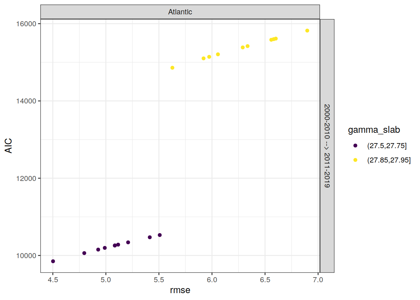
| Version | Author | Date |
|---|---|---|
| 83a13de | jens-daniel-mueller | 2021-03-20 |
| cf98c6d | jens-daniel-mueller | 2021-03-16 |
| a1d52ff | jens-daniel-mueller | 2021-03-15 |
| 0bade3b | jens-daniel-mueller | 2021-03-15 |
| 27c1f4b | jens-daniel-mueller | 2021-03-14 |
| af75ebf | jens-daniel-mueller | 2021-03-14 |
| 5017709 | jens-daniel-mueller | 2021-03-11 |
| 585b07f | jens-daniel-mueller | 2021-03-11 |
| 85a5ed2 | jens-daniel-mueller | 2021-03-10 |
| 6c0bec6 | jens-daniel-mueller | 2021-03-05 |
| 3c2ec33 | jens-daniel-mueller | 2021-03-05 |
| af70b94 | jens-daniel-mueller | 2021-03-04 |
| ac1a836 | jens-daniel-mueller | 2021-02-24 |
| b03fbd3 | jens-daniel-mueller | 2021-02-24 |
| 3d3b4cc | jens-daniel-mueller | 2021-02-23 |
| 7b672f7 | jens-daniel-mueller | 2021-01-11 |
| 33ba23c | jens-daniel-mueller | 2021-01-07 |
| 318609d | jens-daniel-mueller | 2020-12-23 |
| 9d0b2d0 | jens-daniel-mueller | 2020-12-23 |
| 0aa2b50 | jens-daniel-mueller | 2020-12-23 |
| 2886da0 | jens-daniel-mueller | 2020-12-19 |
| 02f0ee9 | jens-daniel-mueller | 2020-12-18 |
| 7bcb4eb | jens-daniel-mueller | 2020-12-18 |
| 7131186 | jens-daniel-mueller | 2020-12-17 |
| 5b48ef5 | jens-daniel-mueller | 2020-12-17 |
7.4.2 BIC
BIC is an alternative criterion to RMSE to judge model quality, but not (yet) taken into account.
lm_all_eras %>%
  ggplot(aes(rmse, BIC, col = gamma_slab)) +
  geom_point() +
  scale_color_viridis_d() +
  facet_grid(eras~basin)
lm_best_eras %>%
  ggplot(aes(rmse, BIC, col = gamma_slab)) +
  geom_point() +
  scale_color_viridis_d() +
  facet_grid(eras~basin)
7.4.3 AIC vs BIC
BIC is an alternative criterion to RMSE to judge model quality, but not (yet) taken into account.
lm_all_eras %>%
  ggplot(aes(AIC, BIC, col = gamma_slab)) +
  geom_point() +
  scale_color_viridis_d() +
  facet_grid(eras~basin)
lm_best_eras %>%
  ggplot(aes(AIC, BIC, col = gamma_slab)) +
  geom_point() +
  scale_color_viridis_d() +
  facet_grid(eras~basin)
7.5 RMSE vs VIF
GLODAP_glanced %>%
  ggplot(aes(rmse, log10(vif_max))) +
  geom_hline(yintercept = 1) +
  geom_point() +
  scale_color_viridis_d() +
  facet_grid(gamma_slab~basin)
7.6 Residual patterns
7.6.1 Fitted vs actual models
Plotted are fitted vs actual target variable values, here: rparams_local$MLR_target`
GLODAP_augmented_best <- left_join(
  lm_best_target %>% select(basin, gamma_slab, era, model),
  GLODAP_augmented
)
# calculate equal axis limits and binwidth
axis_lims <- GLODAP_augmented %>%
summarise(
max_value = max(
c(max(.fitted, max(!!sym(params_local$MLR_target))))
),
min_value = min(
c(min(.fitted, min(!!sym(params_local$MLR_target))))
)
)
i_binwidth <- 1
# binwidth_value <- (axis_lims$max_value - axis_lims$min_value) / 40
axis_lims <- c(axis_lims$min_value, axis_lims$max_value)
GLODAP_augmented %>%
ggplot(aes(cstar_tref, .fitted)) +
geom_bin2d(binwidth = i_binwidth) +
scale_fill_viridis_c() +
geom_abline(slope = 1,
col = 'red') +
coord_equal(xlim = axis_lims,
ylim = axis_lims) +
labs(title = "All models")
| Version | Author | Date |
|---|---|---|
| 83a13de | jens-daniel-mueller | 2021-03-20 |
| cf98c6d | jens-daniel-mueller | 2021-03-16 |
| a1d52ff | jens-daniel-mueller | 2021-03-15 |
| 0bade3b | jens-daniel-mueller | 2021-03-15 |
| 27c1f4b | jens-daniel-mueller | 2021-03-14 |
| af75ebf | jens-daniel-mueller | 2021-03-14 |
| 5017709 | jens-daniel-mueller | 2021-03-11 |
| 585b07f | jens-daniel-mueller | 2021-03-11 |
| 85a5ed2 | jens-daniel-mueller | 2021-03-10 |
| 6c0bec6 | jens-daniel-mueller | 2021-03-05 |
| 3c2ec33 | jens-daniel-mueller | 2021-03-05 |
| af70b94 | jens-daniel-mueller | 2021-03-04 |
| 27ae473 | jens-daniel-mueller | 2021-02-24 |
| 4bc00ea | jens-daniel-mueller | 2021-02-24 |
GLODAP_augmented_best %>%
  ggplot(aes(cstar_tref, .fitted)) +
  geom_bin2d(binwidth = i_binwidth) +
  scale_fill_viridis_c() +
  geom_abline(slope = 1,
              col = 'red') +
  coord_equal(xlim = axis_lims,
              ylim = axis_lims) +
  labs(title = "Selected models")
| Version | Author | Date |
|---|---|---|
| 83a13de | jens-daniel-mueller | 2021-03-20 |
| cf98c6d | jens-daniel-mueller | 2021-03-16 |
| a1d52ff | jens-daniel-mueller | 2021-03-15 |
| 0bade3b | jens-daniel-mueller | 2021-03-15 |
| 27c1f4b | jens-daniel-mueller | 2021-03-14 |
| af75ebf | jens-daniel-mueller | 2021-03-14 |
| 5017709 | jens-daniel-mueller | 2021-03-11 |
| 585b07f | jens-daniel-mueller | 2021-03-11 |
| 85a5ed2 | jens-daniel-mueller | 2021-03-10 |
| 6c0bec6 | jens-daniel-mueller | 2021-03-05 |
| 3c2ec33 | jens-daniel-mueller | 2021-03-05 |
| af70b94 | jens-daniel-mueller | 2021-03-04 |
| 27ae473 | jens-daniel-mueller | 2021-02-24 |
| 4bc00ea | jens-daniel-mueller | 2021-02-24 |
rm(binwidth_value, axis_lims)7.6.2 Pooled
In the following, we present residual patterns vs latitude across all domains.
i_ylim <- c(-30,30)

GLODAP_augmented_best %>%
  ggplot(aes(lat, .resid)) +
  geom_bin2d(binwidth = i_binwidth) +
  geom_hline(yintercept = 0, col = "white") +
  scale_fill_viridis_c() +
  labs(
    title = paste(
      "Target variable:",
      params_local$MLR_target,
      "| Selected models",
      "| All domains"
    )
  )
| Version | Author | Date |
|---|---|---|
| 83a13de | jens-daniel-mueller | 2021-03-20 |
| cf98c6d | jens-daniel-mueller | 2021-03-16 |
| a1d52ff | jens-daniel-mueller | 2021-03-15 |
| 0bade3b | jens-daniel-mueller | 2021-03-15 |
| 27c1f4b | jens-daniel-mueller | 2021-03-14 |
| af75ebf | jens-daniel-mueller | 2021-03-14 |
| 5017709 | jens-daniel-mueller | 2021-03-11 |
| 585b07f | jens-daniel-mueller | 2021-03-11 |
| 85a5ed2 | jens-daniel-mueller | 2021-03-10 |
| 6c0bec6 | jens-daniel-mueller | 2021-03-05 |
| 3c2ec33 | jens-daniel-mueller | 2021-03-05 |
| af70b94 | jens-daniel-mueller | 2021-03-04 |
| 27ae473 | jens-daniel-mueller | 2021-02-24 |
| 4bc00ea | jens-daniel-mueller | 2021-02-24 |
Due to the few large residuals, we limit the y axis range for the plots below.
GLODAP_augmented_best %>%
  ggplot(aes(lat, .resid)) +
  geom_bin2d(binwidth = i_binwidth) +
  geom_hline(yintercept = 0, col = "white") +
  scale_fill_viridis_c() +
  coord_cartesian(ylim = i_ylim) +
  labs(
    title = paste(
      "Target variable:",
      params_local$MLR_target,
      "| Selected models",
      "| All domains"
    )
  )
| Version | Author | Date |
|---|---|---|
| 83a13de | jens-daniel-mueller | 2021-03-20 |
| cf98c6d | jens-daniel-mueller | 2021-03-16 |
| a1d52ff | jens-daniel-mueller | 2021-03-15 |
| 0bade3b | jens-daniel-mueller | 2021-03-15 |
| 27c1f4b | jens-daniel-mueller | 2021-03-14 |
| af75ebf | jens-daniel-mueller | 2021-03-14 |
| 5017709 | jens-daniel-mueller | 2021-03-11 |
| 585b07f | jens-daniel-mueller | 2021-03-11 |
| 85a5ed2 | jens-daniel-mueller | 2021-03-10 |
| 6c0bec6 | jens-daniel-mueller | 2021-03-05 |
| 3c2ec33 | jens-daniel-mueller | 2021-03-05 |
| af70b94 | jens-daniel-mueller | 2021-03-04 |
| 27ae473 | jens-daniel-mueller | 2021-02-24 |
| 4bc00ea | jens-daniel-mueller | 2021-02-24 |
7.6.3 By model domain
In the following, we present residual patterns vs latitude for separate model domains, ie basins, density slabs and eras.
p_residuals <- function(df){
    ggplot(data = df, aes(lat, .resid)) +
      geom_bin2d(binwidth = i_binwidth) +
      geom_hline(yintercept = 0, col = "black") +
      scale_fill_viridis_c() +
      facet_grid(gamma_slab ~ era) +
      coord_cartesian(ylim = i_ylim) +
      labs(
        title = paste(
          "Target variable:",
          params_local$MLR_target,
          "| selected best models | basin:",
          unique(df$basin)
        )
      )
}

GLODAP_augmented_best %>%
  group_split(basin) %>%
  map(p_residuals)
[[1]]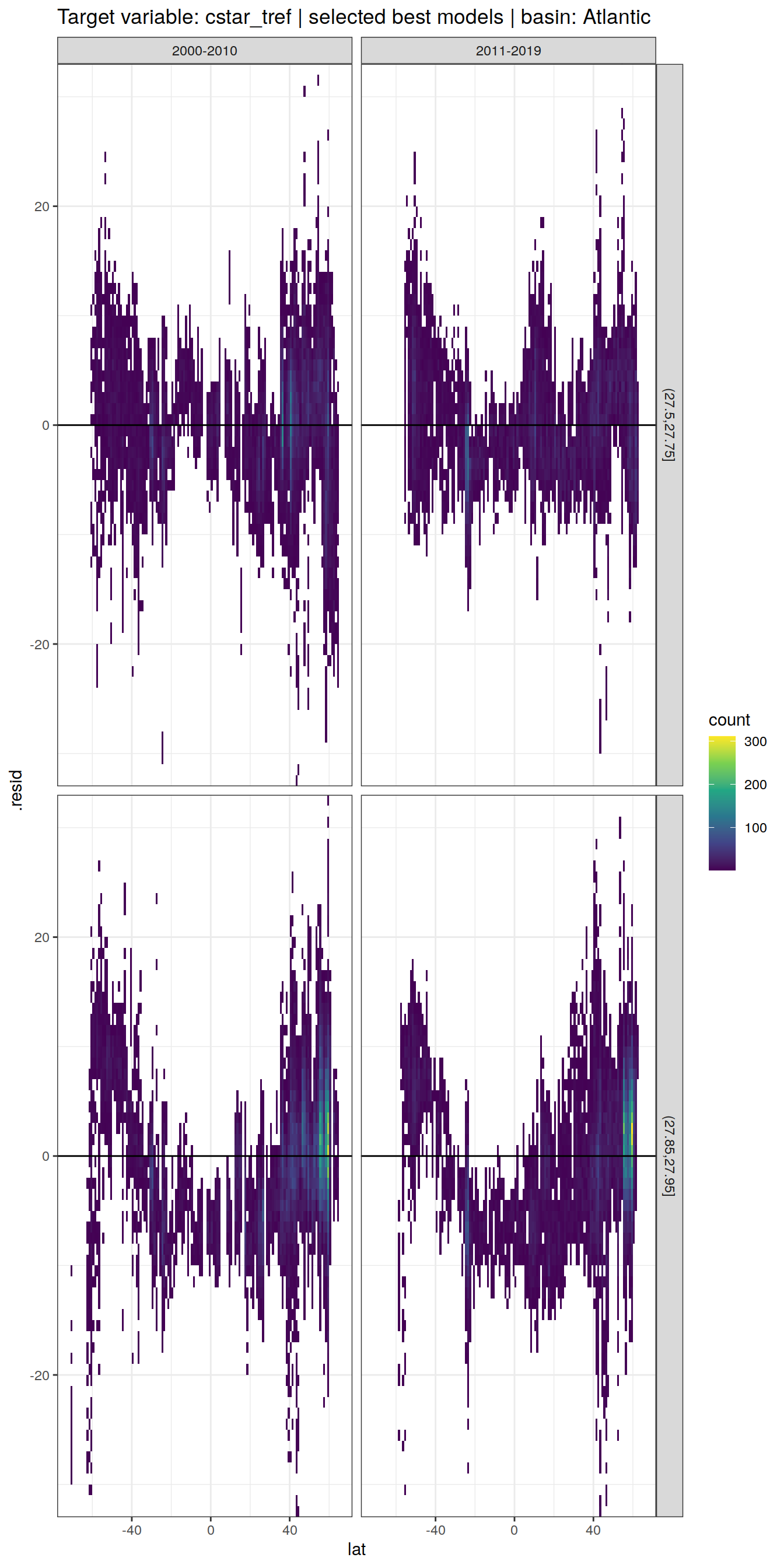
| Version | Author | Date |
|---|---|---|
| 83a13de | jens-daniel-mueller | 2021-03-20 |
| cf98c6d | jens-daniel-mueller | 2021-03-16 |
| a1d52ff | jens-daniel-mueller | 2021-03-15 |
| 0bade3b | jens-daniel-mueller | 2021-03-15 |
| 27c1f4b | jens-daniel-mueller | 2021-03-14 |
| af75ebf | jens-daniel-mueller | 2021-03-14 |
| 5017709 | jens-daniel-mueller | 2021-03-11 |
| 585b07f | jens-daniel-mueller | 2021-03-11 |
| 85a5ed2 | jens-daniel-mueller | 2021-03-10 |
| 6c0bec6 | jens-daniel-mueller | 2021-03-05 |
| 3c2ec33 | jens-daniel-mueller | 2021-03-05 |
| af70b94 | jens-daniel-mueller | 2021-03-04 |
| 27ae473 | jens-daniel-mueller | 2021-02-24 |
| a1ba577 | jens-daniel-mueller | 2021-02-24 |
| 071743d | jens-daniel-mueller | 2021-02-24 |
7.6.4 Latitudinal mean
GLODAP_augmented_best <- GLODAP_augmented_best %>%
  mutate(lat_grid = as.numeric(as.character(cut(
    lat,
    seq(-90, 90, 10),
    seq(-85, 85, 10)
  ))))

lat_residual <- GLODAP_augmented_best %>%
  group_by(basin, gamma_slab, era, lat_grid) %>%
  summarise(.resid_mean = mean(.resid)) %>%
  ungroup()

lat_residual %>%
  ggplot(aes(lat_grid, .resid_mean, col=era)) +
  geom_line() +
  geom_point() +
  geom_hline(yintercept = 0, col = "black") +
  facet_grid(gamma_slab ~ basin)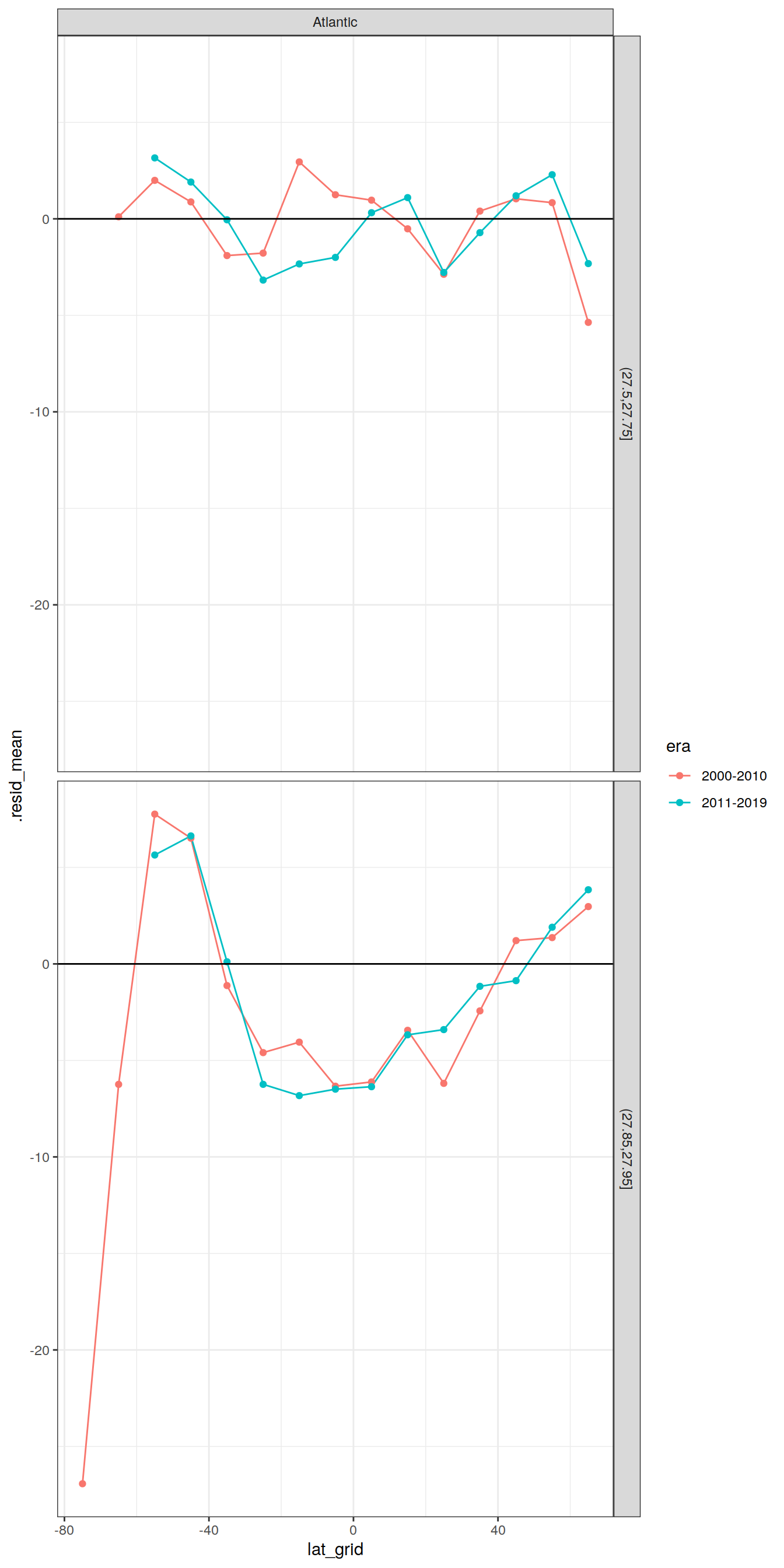
| Version | Author | Date |
|---|---|---|
| 83a13de | jens-daniel-mueller | 2021-03-20 |
| cf98c6d | jens-daniel-mueller | 2021-03-16 |
| a1d52ff | jens-daniel-mueller | 2021-03-15 |
| 0bade3b | jens-daniel-mueller | 2021-03-15 |
| 27c1f4b | jens-daniel-mueller | 2021-03-14 |
| af75ebf | jens-daniel-mueller | 2021-03-14 |
| 5017709 | jens-daniel-mueller | 2021-03-11 |
| 585b07f | jens-daniel-mueller | 2021-03-11 |
| 85a5ed2 | jens-daniel-mueller | 2021-03-10 |
| 6c0bec6 | jens-daniel-mueller | 2021-03-05 |
| 3c2ec33 | jens-daniel-mueller | 2021-03-05 |
| af70b94 | jens-daniel-mueller | 2021-03-04 |
| fec3558 | jens-daniel-mueller | 2021-02-24 |
7.6.5 Latitudinal offset
# calculate residual offset for adjacent eras
lat_residual_offset <- lat_residual  %>%
  select(basin, gamma_slab, era, lat_grid, .resid_mean) %>%
  arrange(era) %>%
  group_by(basin, gamma_slab, lat_grid) %>%
  mutate(eras = paste(lag(era), era, sep = " --> "),
         .resid_mean_offset = .resid_mean - lag(.resid_mean)
         ) %>%
  ungroup() %>%
  select(-era) %>%
  drop_na() %>%
  filter(eras != paste(unique(lat_residual$era)[1],
                       unique(lat_residual$era)[3],
                       sep = " --> "))

lat_residual_offset %>%
  ggplot(aes(lat_grid, .resid_mean_offset, col=eras)) +
  geom_line() +
  geom_point() +
  geom_hline(yintercept = 0, col = "black") +
  facet_grid(gamma_slab ~ basin)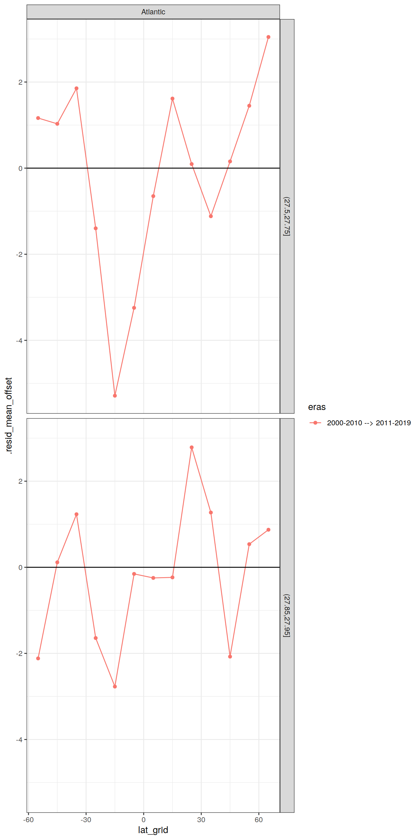
| Version | Author | Date |
|---|---|---|
| 83a13de | jens-daniel-mueller | 2021-03-20 |
| cf98c6d | jens-daniel-mueller | 2021-03-16 |
| a1d52ff | jens-daniel-mueller | 2021-03-15 |
| 0bade3b | jens-daniel-mueller | 2021-03-15 |
| 27c1f4b | jens-daniel-mueller | 2021-03-14 |
| af75ebf | jens-daniel-mueller | 2021-03-14 |
| 5017709 | jens-daniel-mueller | 2021-03-11 |
| 585b07f | jens-daniel-mueller | 2021-03-11 |
| 85a5ed2 | jens-daniel-mueller | 2021-03-10 |
| 6c0bec6 | jens-daniel-mueller | 2021-03-05 |
| 3c2ec33 | jens-daniel-mueller | 2021-03-05 |
| af70b94 | jens-daniel-mueller | 2021-03-04 |
| fec3558 | jens-daniel-mueller | 2021-02-24 |
8 VIF
GLODAP_glanced %>%
  ggplot(aes(as.factor(n), log10(vif_max))) +
  geom_hline(yintercept = log10(params_local$vif_max)) +
  geom_violin() +
  facet_grid(gamma_slab~basin)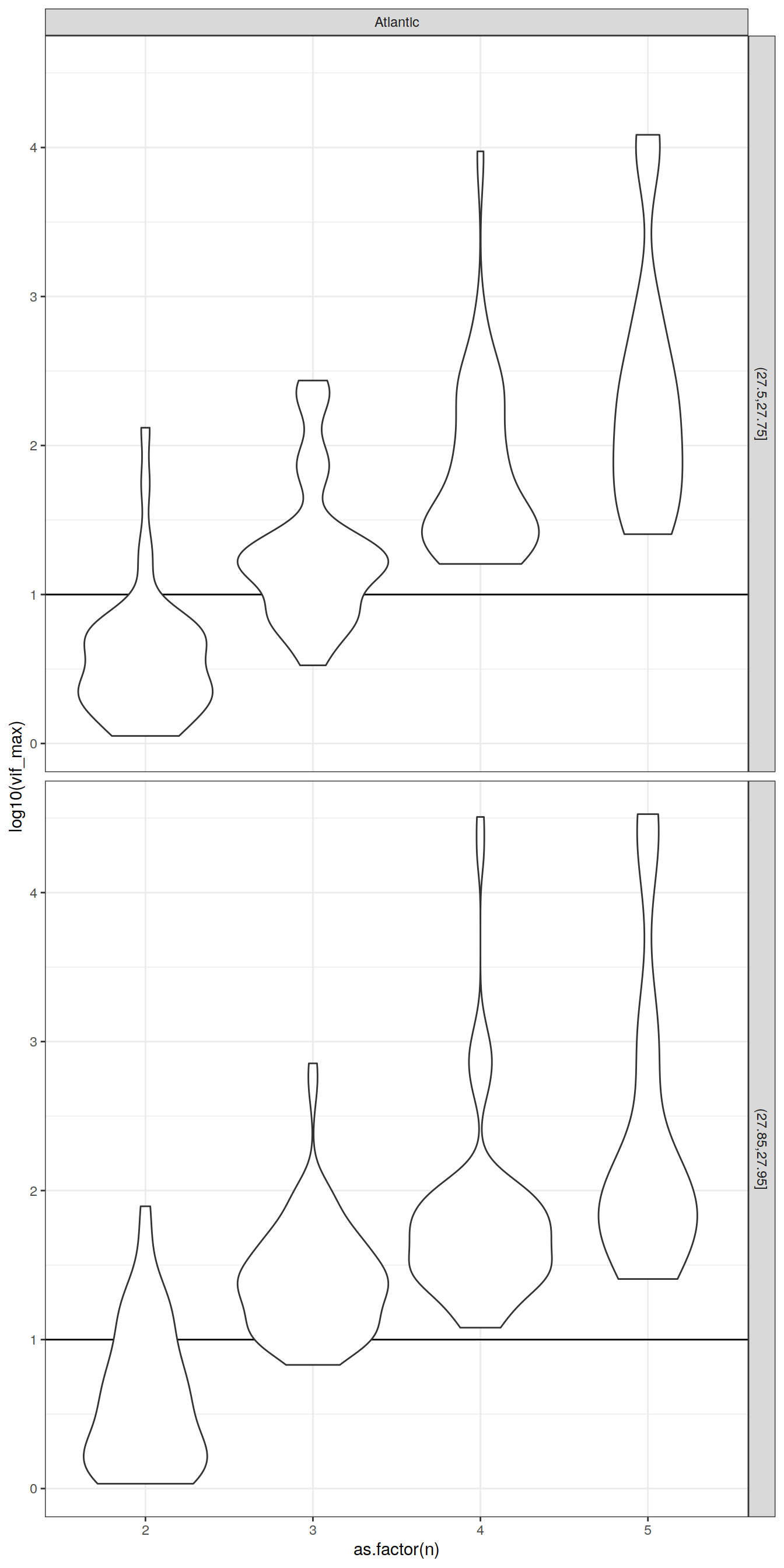
| Version | Author | Date |
|---|---|---|
| 330dcd0 | jens-daniel-mueller | 2021-03-20 |
GLODAP_glanced_vif %>%
  ggplot(aes(Variables, log10(VIF))) +
  geom_hline(yintercept = log10(params_local$vif_max)) +
  geom_violin() +
  # geom_point(shape = 21) +
  facet_grid(gamma_slab~basin) +
  coord_flip()
| Version | Author | Date |
|---|---|---|
| 330dcd0 | jens-daniel-mueller | 2021-03-20 |
sessionInfo()R version 4.0.3 (2020-10-10)
Platform: x86_64-pc-linux-gnu (64-bit)
Running under: openSUSE Leap 15.2
Matrix products: default
BLAS: /usr/local/R-4.0.3/lib64/R/lib/libRblas.so
LAPACK: /usr/local/R-4.0.3/lib64/R/lib/libRlapack.so
locale:
[1] LC_CTYPE=en_US.UTF-8 LC_NUMERIC=C
[3] LC_TIME=en_US.UTF-8 LC_COLLATE=en_US.UTF-8
[5] LC_MONETARY=en_US.UTF-8 LC_MESSAGES=en_US.UTF-8
[7] LC_PAPER=en_US.UTF-8 LC_NAME=C
[9] LC_ADDRESS=C LC_TELEPHONE=C
[11] LC_MEASUREMENT=en_US.UTF-8 LC_IDENTIFICATION=C
attached base packages:
[1] stats graphics grDevices utils datasets methods base
other attached packages:
[1] gt_0.2.2 corrr_0.4.3 broom_0.7.2 kableExtra_1.3.1
[5] knitr_1.30 olsrr_0.5.3 GGally_2.0.0 lubridate_1.7.9
[9] metR_0.9.0 scico_1.2.0 patchwork_1.1.1 collapse_1.5.0
[13] forcats_0.5.0 stringr_1.4.0 dplyr_1.0.2 purrr_0.3.4
[17] readr_1.4.0 tidyr_1.1.2 tibble_3.0.4 ggplot2_3.3.2
[21] tidyverse_1.3.0 workflowr_1.6.2
loaded via a namespace (and not attached):
[1] fs_1.5.0 webshot_0.5.2 RColorBrewer_1.1-2
[4] httr_1.4.2 rprojroot_2.0.2 tools_4.0.3
[7] backports_1.1.10 utf8_1.1.4 R6_2.5.0
[10] nortest_1.0-4 DBI_1.1.0 colorspace_1.4-1
[13] withr_2.3.0 gridExtra_2.3 tidyselect_1.1.0
[16] curl_4.3 compiler_4.0.3 git2r_0.27.1
[19] cli_2.1.0 rvest_0.3.6 xml2_1.3.2
[22] sass_0.2.0 labeling_0.4.2 scales_1.1.1
[25] checkmate_2.0.0 goftest_1.2-2 digest_0.6.27
[28] foreign_0.8-80 rmarkdown_2.5 rio_0.5.16
[31] pkgconfig_2.0.3 htmltools_0.5.0 highr_0.8
[34] dbplyr_1.4.4 rlang_0.4.9 readxl_1.3.1
[37] rstudioapi_0.13 farver_2.0.3 generics_0.0.2
[40] jsonlite_1.7.1 zip_2.1.1 car_3.0-10
[43] magrittr_1.5 Matrix_1.2-18 Rcpp_1.0.5
[46] munsell_0.5.0 fansi_0.4.1 abind_1.4-5
[49] lifecycle_0.2.0 stringi_1.5.3 whisker_0.4
[52] yaml_2.2.1 carData_3.0-4 plyr_1.8.6
[55] grid_4.0.3 blob_1.2.1 parallel_4.0.3
[58] promises_1.1.1 crayon_1.3.4 lattice_0.20-41
[61] haven_2.3.1 hms_0.5.3 pillar_1.4.7
[64] reprex_0.3.0 glue_1.4.2 evaluate_0.14
[67] RcppArmadillo_0.10.1.2.0 data.table_1.13.2 modelr_0.1.8
[70] vctrs_0.3.5 httpuv_1.5.4 cellranger_1.1.0
[73] gtable_0.3.0 reshape_0.8.8 assertthat_0.2.1
[76] xfun_0.18 openxlsx_4.2.3 RcppEigen_0.3.3.7.0
[79] later_1.1.0.1 viridisLite_0.3.0 ellipsis_0.3.1
[82] here_0.1