Last updated: 2020-12-15

Checks: 7 0

Knit directory: emlr_obs_v_XXX/

This reproducible R Markdown analysis was created with workflowr (version 1.6.2). The Checks tab describes the reproducibility checks that were applied when the results were created. The Past versions tab lists the development history.

R Markdown file: up-to-date

Great! Since the R Markdown file has been committed to the Git repository, you know the exact version of the code that produced these results.

Environment: empty

Great job! The global environment was empty. Objects defined in the global environment can affect the analysis in your R Markdown file in unknown ways. For reproduciblity it’s best to always run the code in an empty environment.

Seed: set.seed(20200707)

The command set.seed(20200707) was run prior to running the code in the R Markdown file. Setting a seed ensures that any results that rely on randomness, e.g. subsampling or permutations, are reproducible.

Session information: recorded

Great job! Recording the operating system, R version, and package versions is critical for reproducibility.

Cache: none

Nice! There were no cached chunks for this analysis, so you can be confident that you successfully produced the results during this run.

File paths: relative

Great job! Using relative paths to the files within your workflowr project makes it easier to run your code on other machines.

Repository version: 449195a

Great! You are using Git for version control. Tracking code development and connecting the code version to the results is critical for reproducibility.

The results in this page were generated with repository version 449195a. See the Past versions tab to see a history of the changes made to the R Markdown and HTML files.

Note that you need to be careful to ensure that all relevant files for the analysis have been committed to Git prior to generating the results (you can use wflow_publish or wflow_git_commit). workflowr only checks the R Markdown file, but you know if there are other scripts or data files that it depends on. Below is the status of the Git repository when the results were generated:


Ignored files:
    Ignored:    .Rhistory
    Ignored:    .Rproj.user/

Unstaged changes:
    Modified:   analysis/_site.yml
    Deleted:    analysis/mapping_cant_calculation.Rmd
    Deleted:    analysis/mapping_cstar_calculation.Rmd
    Modified:   code/Workflowr_project_managment.R
    Modified:   data/auxillary/params_local.rds

Note that any generated files, e.g. HTML, png, CSS, etc., are not included in this status report because it is ok for generated content to have uncommitted changes.

These are the previous versions of the repository in which changes were made to the R Markdown (analysis/eMLR_data_preparation.Rmd) and HTML (docs/eMLR_data_preparation.html) files. If you’ve configured a remote Git repository (see ?wflow_git_remote), click on the hyperlinks in the table below to view the files as they were in that past version.

File	Version	Author	Date	Message
Rmd	449195a	jens-daniel-mueller	2020-12-15	rebuild without subsetting nitrate
html	7a9a4cb	jens-daniel-mueller	2020-12-15	Build site.
Rmd	d234226	jens-daniel-mueller	2020-12-15	rebuild with cstar_tref
html	61b263c	jens-daniel-mueller	2020-12-15	Build site.
html	4d612dd	jens-daniel-mueller	2020-12-15	Build site.
Rmd	e7e5ff1	jens-daniel-mueller	2020-12-15	rebuild with eMLR target variable selection
html	953caf3	jens-daniel-mueller	2020-12-15	Build site.
html	42daf5c	jens-daniel-mueller	2020-12-14	Build site.
Rmd	923aa7f	jens-daniel-mueller	2020-12-14	rebuild with new path and auto folder creation
html	984697e	jens-daniel-mueller	2020-12-12	Build site.
html	3ebff89	jens-daniel-mueller	2020-12-12	Build site.
html	7d82772	jens-daniel-mueller	2020-12-11	Build site.
Rmd	6069c23	jens-daniel-mueller	2020-12-11	selectable basinmask, try 5
html	7788175	jens-daniel-mueller	2020-12-09	Build site.
Rmd	64b795c	jens-daniel-mueller	2020-12-09	added histograms after data preparation
html	b01a367	jens-daniel-mueller	2020-12-09	Build site.
html	24a632f	jens-daniel-mueller	2020-12-07	Build site.
html	92dca91	jens-daniel-mueller	2020-12-07	Build site.
html	6a8004b	jens-daniel-mueller	2020-12-07	Build site.
html	70bf1a5	jens-daniel-mueller	2020-12-07	Build site.
html	7555355	jens-daniel-mueller	2020-12-07	Build site.
html	143d6fa	jens-daniel-mueller	2020-12-07	Build site.
html	3c8a83c	jens-daniel-mueller	2020-12-04	Build site.
Rmd	e11f455	jens-daniel-mueller	2020-12-04	improved output plots by using stat_2d instead of points
html	abc6818	jens-daniel-mueller	2020-12-03	Build site.
Rmd	992ba15	jens-daniel-mueller	2020-12-03	rebuild with variable inventory depth
html	090e4d5	jens-daniel-mueller	2020-12-02	Build site.
Rmd	c98d27b	jens-daniel-mueller	2020-12-02	cleaned subsetting and data preparation
html	37e9dac	jens-daniel-mueller	2020-12-02	Build site.
Rmd	9ff071b	jens-daniel-mueller	2020-12-02	minor improvement of tref adejustment, formatting
html	7c25f7a	jens-daniel-mueller	2020-12-02	Build site.
html	ec8dc38	jens-daniel-mueller	2020-12-02	Build site.
html	c987de1	jens-daniel-mueller	2020-12-02	Build site.
html	f8358f8	jens-daniel-mueller	2020-12-02	Build site.
html	b03ddb8	jens-daniel-mueller	2020-12-02	Build site.
Rmd	9183e8f	jens-daniel-mueller	2020-12-02	revised assignment of era to eras
html	22d0127	jens-daniel-mueller	2020-12-01	Build site.
html	0ff728b	jens-daniel-mueller	2020-12-01	Build site.
html	b02b7a4	jens-daniel-mueller	2020-12-01	Build site.
Rmd	60bea48	jens-daniel-mueller	2020-12-01	auto eras naming
html	cf19652	jens-daniel-mueller	2020-11-30	Build site.
Rmd	2842970	jens-daniel-mueller	2020-11-30	cleaned for eMLR part only
html	196be51	jens-daniel-mueller	2020-11-30	Build site.
Rmd	7a4b015	jens-daniel-mueller	2020-11-30	first rebuild on ETH server
Rmd	bc61ce3	Jens Müller	2020-11-30	Initial commit
html	bc61ce3	Jens Müller	2020-11-30	Initial commit

1 Required data

Required are:

GLODAPv2.2020
- cleaned data file
- horizontal grid of sampling coordinates
Cant from Sabine 2004
annual mean atmospheric pCO₂

GLODAP <-
  read_csv(paste(path_version_data,
                 "GLODAPv2.2020_clean.csv",
                 sep = ""))

GLODAP_obs_grid <-
  read_csv(paste(path_version_data,
                 "GLODAPv2.2020_clean_obs_grid.csv",
                 sep = ""))

S04_cant_3d <-
  read_csv(paste(path_preprocessing,
                 "S04_cant_3d.csv",
                 sep = ""))

co2_atm <-
  read_csv(paste(path_preprocessing,
                 "co2_atm.csv",
                 sep = ""))

2 PO₄*

2.1 Calculation

The predictor PO₄* was be calculated according to Clement and Gruber (2018), ie based on oxygen. Please note that an erroneous equations for PO4* calculation is given in the supplement of Gruber et al (2019), based on nitrate.

Here we use following equation:

print(b_phosphate_star)

function (phosphate, oxygen) 
{
    phosphate_star = phosphate + (oxygen/params_local$rPO) - 
        params_local$rPO_offset
    return(phosphate_star)
}

GLODAP <- GLODAP %>% 
  mutate(phosphate_star = b_phosphate_star(phosphate, oxygen))

3 C*

C* serves as a conservative tracer of anthropogenic CO₂ uptake. It is derived from measured DIC by removing the impact of

organic matter formation and respiration
calcification and calcium carbonate dissolution

Contributions of those processes are estimated from phosphate and alkalinity concentrations.

3.1 Stoichiometric ratios

The stoichiometric nutrient ratios for the production and mineralization of organic matter were set to:

C/P: 117
N/P: 16

3.2 Calculation

C* was calculated as:

print(b_cstar)

function (tco2, phosphate, talk) 
{
    cstar = tco2 - (params_local$rCP * phosphate) - 0.5 * (talk - 
        (params_local$rNP * phosphate))
    return(cstar)
}

GLODAP <- GLODAP %>% 
  mutate(rCP_phosphate = -params_local$rCP * phosphate,
         talk_05 = -0.5 * talk,
         rNP_phosphate_05 = -0.5 * params_local$rNP * phosphate,
         cstar = b_cstar(tco2, phosphate, talk))

3.3 Reference year adjustment

The reference year adjustment relies on an apriori estimate of Cant at a given location and depth, which is used as a scaling factor for the concurrent change in atmospheric CO₂. The underlying assumption is a transient steady state for the oceanic Cant uptake. Here, Cant from the GLODAP mapped Climatology was used.

Note that eq. 6 in Clement and Gruber (2018) misses pCO₂ pre-industrial in the denominator. Here we use the equation published in Gruber et al. (2019).

3.3.1 Combine GLODAP + Cant

S04_cant_3d_obs <- left_join(
  GLODAP_obs_grid,
  S04_cant_3d %>% select(-c(cant, eras))
  )

# calculate number of cant data points per grid cell
S04_cant_3d_obs <- S04_cant_3d_obs %>%
  group_by(lon, lat) %>% 
  mutate(n = n()) %>% 
  ungroup()

# S04_cant_3d_obs %>%
#   filter(n <= 1) %>%
#   ggplot(aes(lon,lat)) +
#   geom_point(data = GLODAP_obs_grid, aes(lon, lat)) +
#   geom_point(col = "red")

rm(S04_cant_3d, GLODAP_obs_grid)

GLODAP_cant_obs <- full_join(GLODAP, S04_cant_3d_obs)

rm(GLODAP, S04_cant_3d_obs)

# fill number of cant data points per grid cell to all observations
GLODAP_cant_obs <- GLODAP_cant_obs %>%
  group_by(lon, lat) %>% 
  fill(n, .direction = "updown") %>% 
  ungroup()

The mapped Cant product was merged with GLODAP observation by:

using an identical 1x1° horizontal grid
linear interpolation of C_ant from standard to sampling depth

# interpolate cant to observation depth
GLODAP_cant_obs_int <- GLODAP_cant_obs %>%
  filter(n > 1) %>% 
  group_by(lat, lon) %>%
  arrange(depth) %>%
  mutate(cant_pos_int = approxfun(depth, cant_pos, rule = 2)(depth)) %>%
  ungroup()

# set cant for observation depth if only one cant available
GLODAP_cant_obs_set <- GLODAP_cant_obs %>%
  filter(n == 1) %>%
  group_by(lat, lon) %>%
  mutate(cant_pos_int = mean(cant_pos, na.rm = TRUE)) %>%
  ungroup()

# bin data sets with interpolated and set cant
GLODAP_cant_obs <- bind_rows(GLODAP_cant_obs_int, GLODAP_cant_obs_set)
rm(GLODAP_cant_obs_int, GLODAP_cant_obs_set)


ggplot() +
  geom_path(
    data = GLODAP_cant_obs %>%
      filter(lat == 48.5, lon == 165.5,!is.na(cant_pos)) %>%
      arrange(depth),
    aes(cant_pos, depth, col = "mapped")
  ) +
  geom_point(
    data = GLODAP_cant_obs %>%
      filter(lat == 48.5, lon == 165.5,!is.na(cant_pos)) %>%
      arrange(depth),
    aes(cant_pos, depth, col = "mapped")
  ) +
  geom_point(
    data = GLODAP_cant_obs %>%
      filter(lat == 48.5, lon == 165.5, date == ymd("2018-06-27")),
    aes(cant_pos_int, depth, col = "interpolated")
  ) +
  scale_y_reverse() +
  scale_color_brewer(palette = "Dark2", name = "") +
  labs(title = "Cant interpolation to sampling depth - example profile")

Version	Author	Date
196be51	jens-daniel-mueller	2020-11-30
bc61ce3	Jens Müller	2020-11-30

# remove cant data at grid cells without observations
GLODAP <- GLODAP_cant_obs %>%
  filter(!is.na(cstar)) %>%
  mutate(cant_pos = cant_pos_int) %>%
  select(-cant_pos_int, n)

rm(GLODAP_cant_obs)

3.3.2 Merge GLODAP + atm. pCO₂

GLODAP observations were merged with mean annual atmospheric pCO₂ levels by year.

GLODAP <- left_join(GLODAP, co2_atm)

3.3.3 Calculation

C_ant for median year of each era was calculated by applying alpha = 0.28/13 * (median year - 1994) to the estimate of Sabine et al. (2004).

# assign reference year
GLODAP <- GLODAP %>% 
  group_by(era) %>% 
  mutate(tref = median(year)) %>% 
  ungroup()

# calculate reference year
tref <- GLODAP %>% 
  group_by(era) %>% 
  summarise(year = median(year)) %>% 
  ungroup()

# extract atm pCO2 at reference year
co2_atm_tref <- right_join(co2_atm, tref) %>% 
  select(-year) %>% 
  rename(pCO2_tref = pCO2)

# merge atm pCO2 at tref with GLODAP
GLODAP <- full_join(GLODAP, co2_atm_tref)
rm(co2_atm, tref)

# scale cant to reference year
GLODAP <- GLODAP %>%
  mutate(alpha = (tref - 1994) * (0.28 / 13),
         cant_pos = cant_pos * (1 + alpha))

# calculate cstar for reference year
GLODAP <- GLODAP %>%
  mutate(
    cstar_tref_delta =
      ((pCO2 - pCO2_tref) / (pCO2_tref - params_local$preind_atm_pCO2)) * cant_pos,
    cstar_tref = cstar - cstar_tref_delta)

3.4 Control plots

GLODAP %>% 
  ggplot(aes(cstar_tref_delta)) +
  geom_histogram(binwidth = 1) +
  labs(title = "Histogramm with binwidth = 1")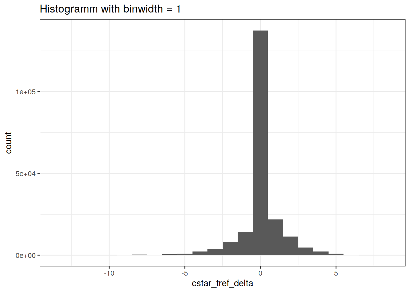

Version	Author	Date
3ebff89	jens-daniel-mueller	2020-12-12
7d82772	jens-daniel-mueller	2020-12-11
7788175	jens-daniel-mueller	2020-12-09
24a632f	jens-daniel-mueller	2020-12-07
6a8004b	jens-daniel-mueller	2020-12-07
70bf1a5	jens-daniel-mueller	2020-12-07
7555355	jens-daniel-mueller	2020-12-07
143d6fa	jens-daniel-mueller	2020-12-07
37e9dac	jens-daniel-mueller	2020-12-02
0ff728b	jens-daniel-mueller	2020-12-01
b02b7a4	jens-daniel-mueller	2020-12-01
196be51	jens-daniel-mueller	2020-11-30
bc61ce3	Jens Müller	2020-11-30

GLODAP %>% 
  sample_n(1e4) %>% 
  ggplot(aes(year, cstar_tref_delta, col = cant_pos)) +
  geom_point() +
  scale_color_viridis_c() +
  labs(title = "Time series of random subsample 1e4")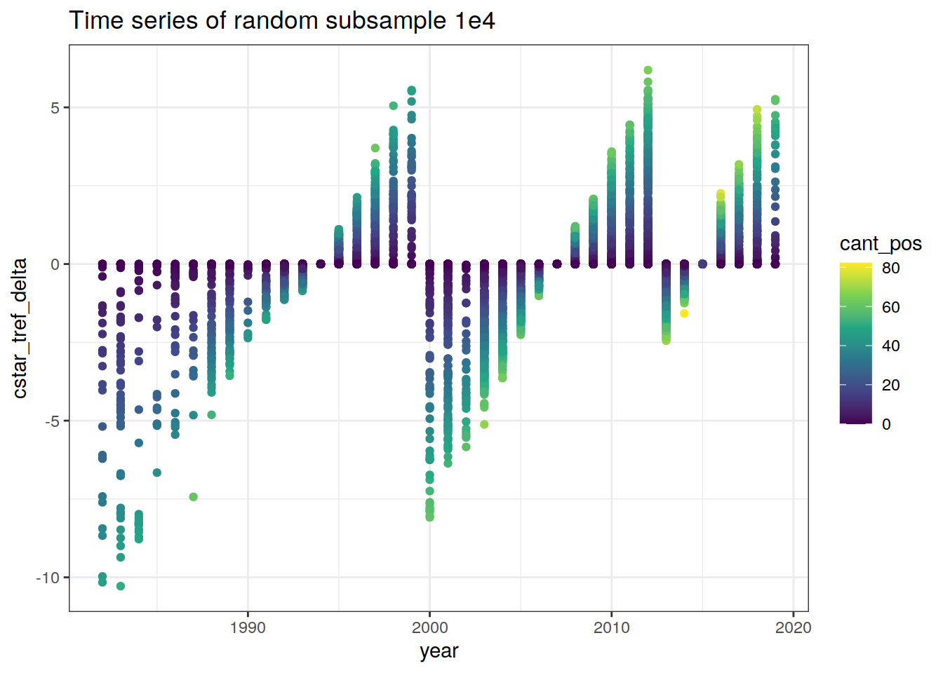

Version	Author	Date
3ebff89	jens-daniel-mueller	2020-12-12
7d82772	jens-daniel-mueller	2020-12-11
7788175	jens-daniel-mueller	2020-12-09
24a632f	jens-daniel-mueller	2020-12-07
6a8004b	jens-daniel-mueller	2020-12-07
70bf1a5	jens-daniel-mueller	2020-12-07
7555355	jens-daniel-mueller	2020-12-07
143d6fa	jens-daniel-mueller	2020-12-07
37e9dac	jens-daniel-mueller	2020-12-02
0ff728b	jens-daniel-mueller	2020-12-01
b02b7a4	jens-daniel-mueller	2020-12-01
196be51	jens-daniel-mueller	2020-11-30
bc61ce3	Jens Müller	2020-11-30

GLODAP %>% 
  ggplot(aes(year, cstar_tref_delta)) +
  geom_bin2d(binwidth = 1) +
  scale_fill_viridis_c(trans = "log10") +
  labs(title = "Heatmap with binwidth = 1")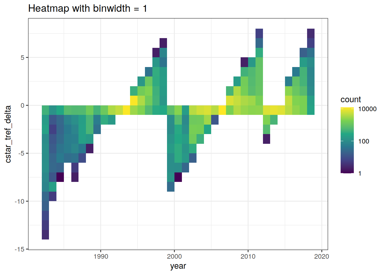

Version	Author	Date
3ebff89	jens-daniel-mueller	2020-12-12
7d82772	jens-daniel-mueller	2020-12-11
7788175	jens-daniel-mueller	2020-12-09
24a632f	jens-daniel-mueller	2020-12-07
6a8004b	jens-daniel-mueller	2020-12-07
70bf1a5	jens-daniel-mueller	2020-12-07
7555355	jens-daniel-mueller	2020-12-07
143d6fa	jens-daniel-mueller	2020-12-07
090e4d5	jens-daniel-mueller	2020-12-02
37e9dac	jens-daniel-mueller	2020-12-02
0ff728b	jens-daniel-mueller	2020-12-01
b02b7a4	jens-daniel-mueller	2020-12-01
196be51	jens-daniel-mueller	2020-11-30
bc61ce3	Jens Müller	2020-11-30

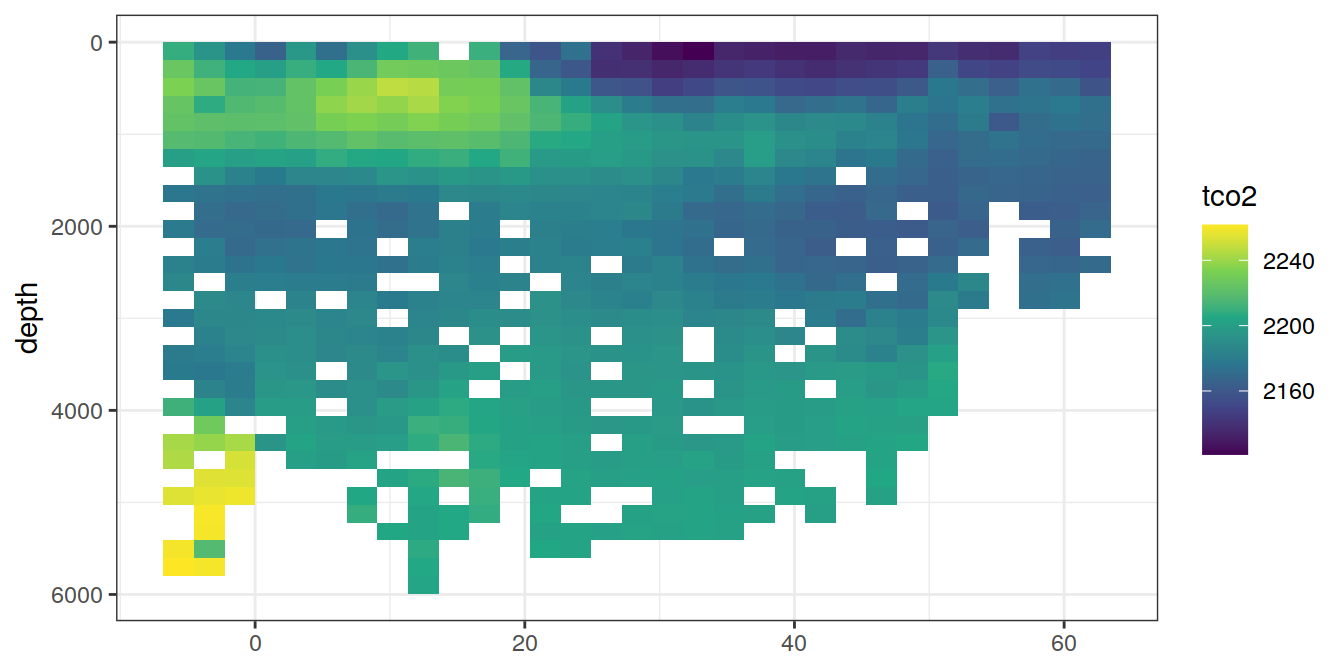
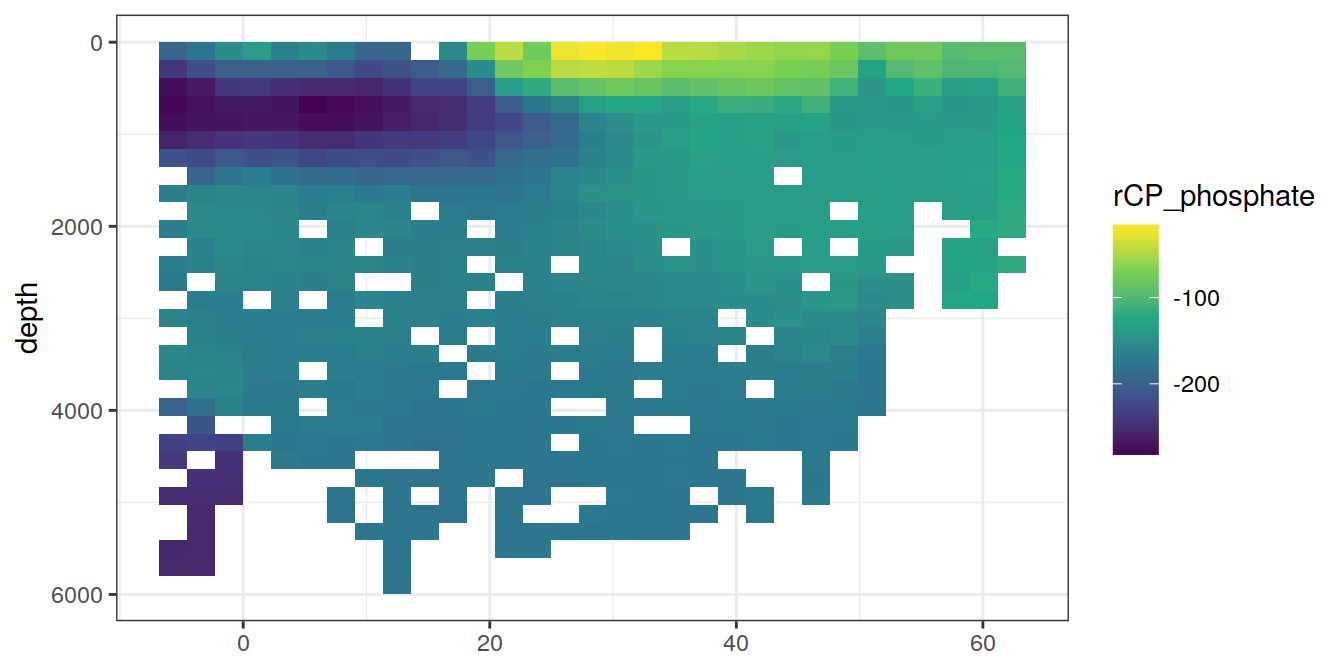
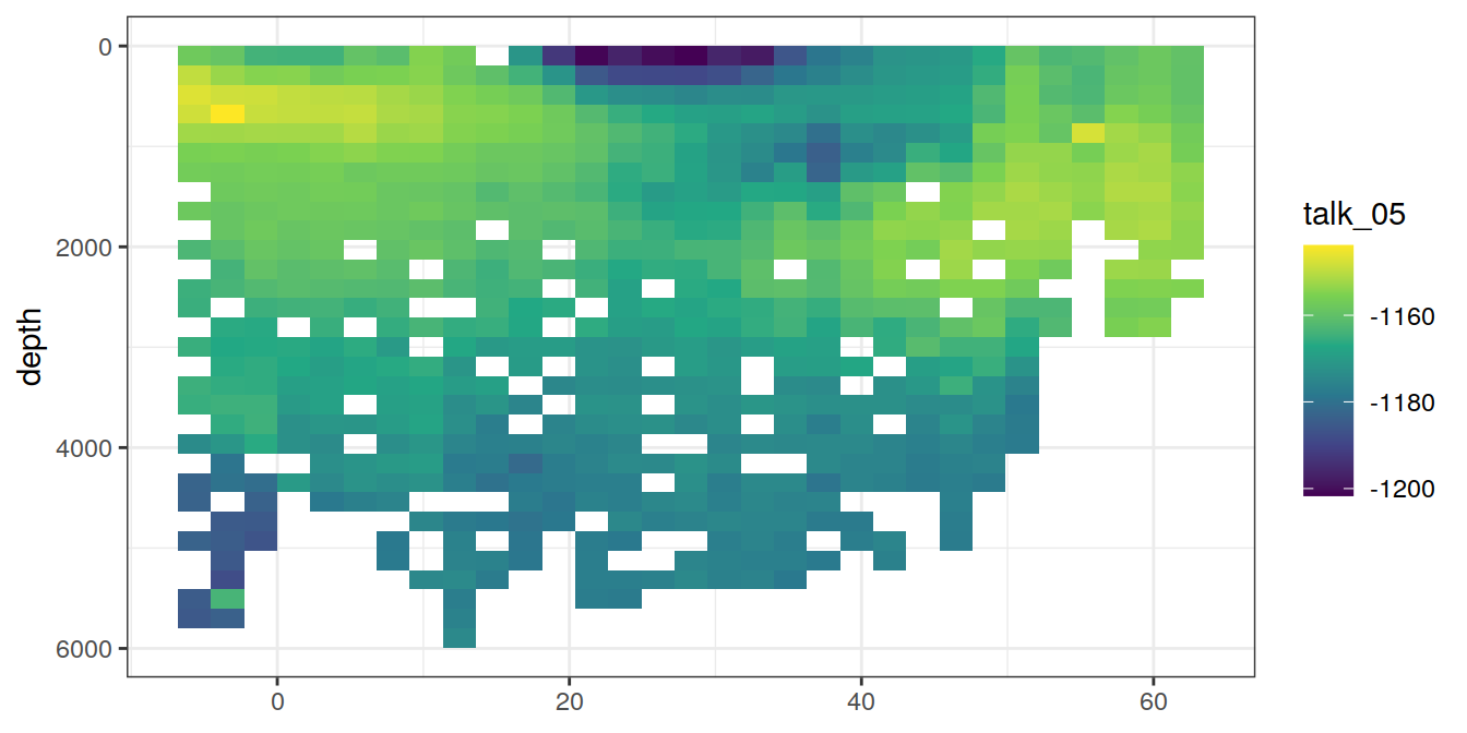
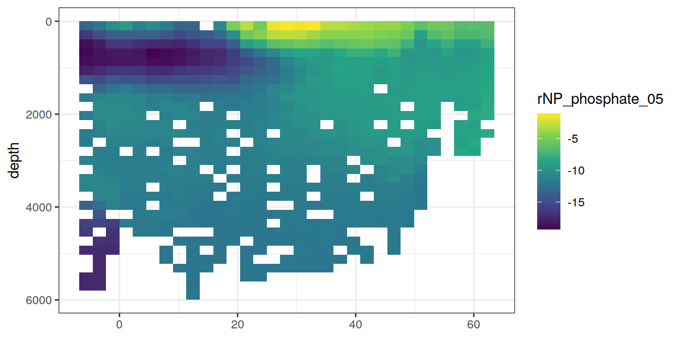
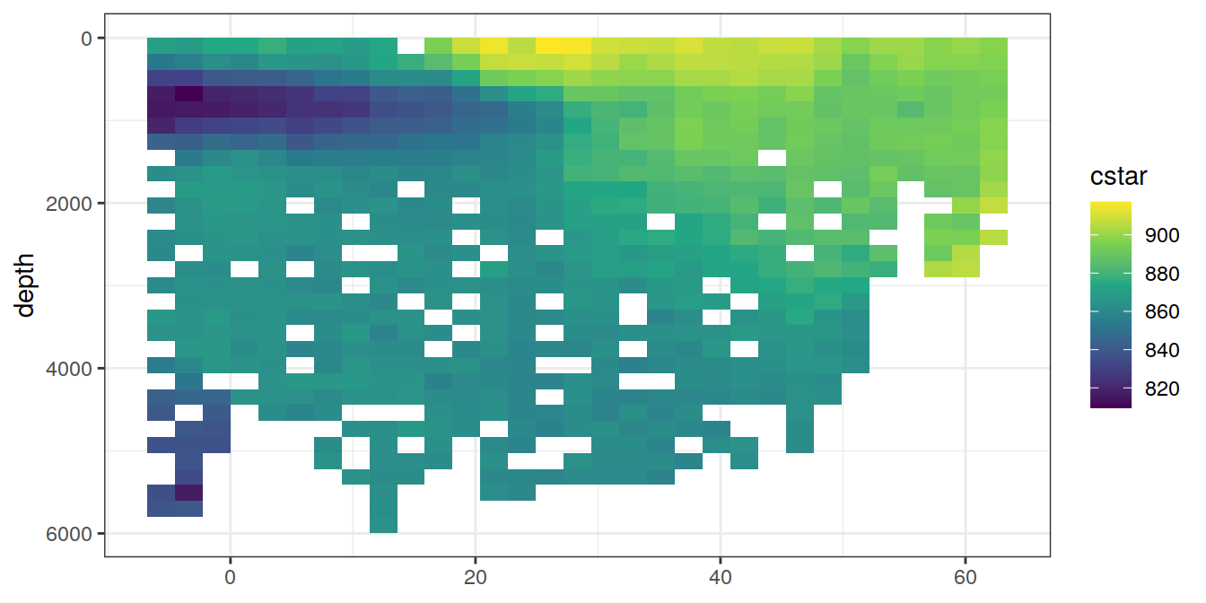
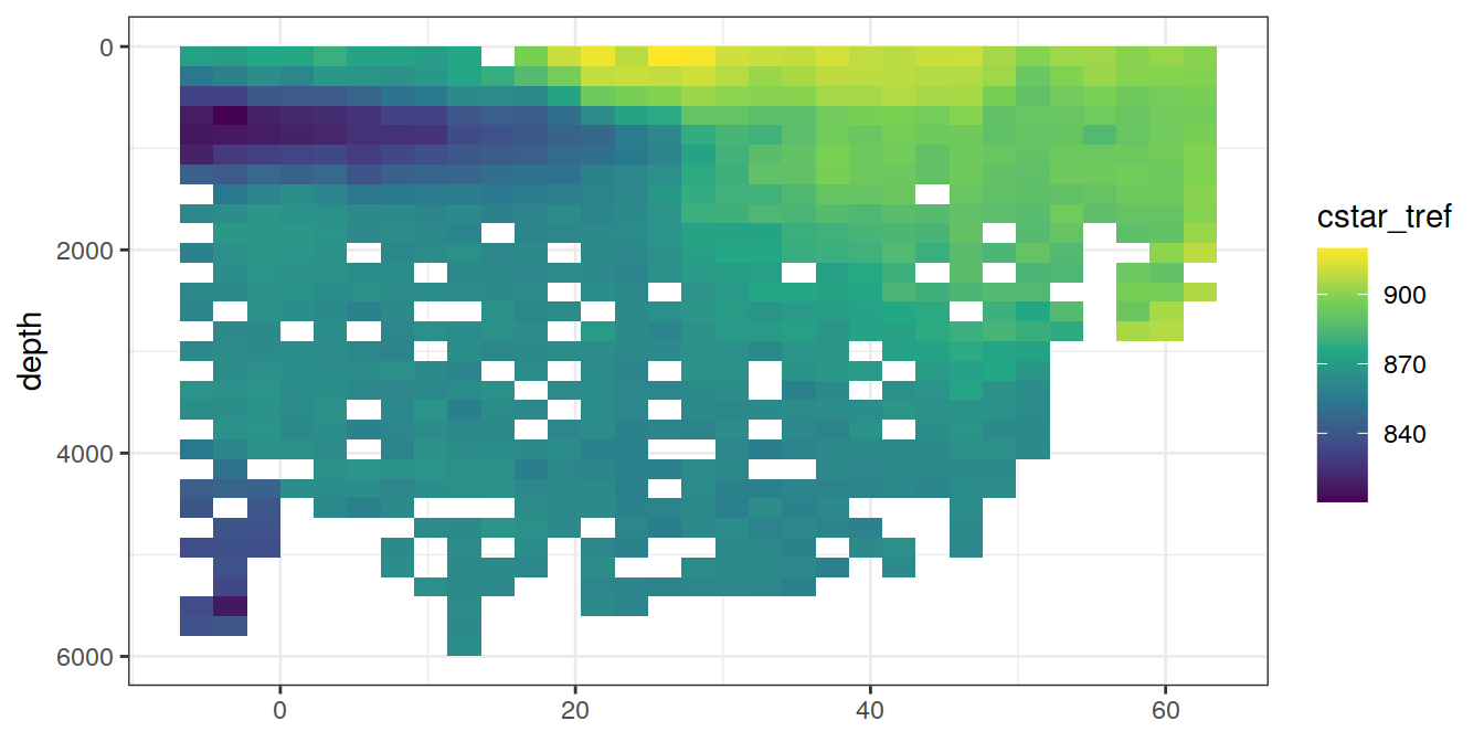
4 Selected section plots

A selected section is plotted to demonstrate the magnitude of various parameters and corrections relevant to C*.

GLODAP_cruise <- GLODAP %>% 
  filter(cruise %in% params_global$cruises_meridional)

map +
  geom_path(data = GLODAP_cruise %>%
              arrange(date),
            aes(lon, lat)) +
  geom_point(data = GLODAP_cruise %>%
              arrange(date),
             aes(lon, lat, col = date)) +
  scale_color_viridis_c(trans = "date") +
  labs(title = paste("Cruise year:", mean(GLODAP_cruise$year)))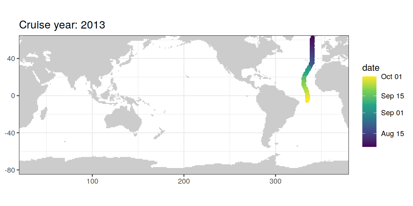

Version	Author	Date
7555355	jens-daniel-mueller	2020-12-07
143d6fa	jens-daniel-mueller	2020-12-07
090e4d5	jens-daniel-mueller	2020-12-02
196be51	jens-daniel-mueller	2020-11-30
bc61ce3	Jens Müller	2020-11-30

lat_section <- 
GLODAP_cruise %>%
  ggplot(aes(lat, depth)) +
  scale_y_reverse() +
  scale_fill_viridis_c() +
  theme(axis.title.x = element_blank())

for (i_var in c("tco2",
                "rCP_phosphate",
                "talk_05",
                "rNP_phosphate_05",
                "cstar",
                "cstar_tref")) {
  print(lat_section +
          stat_summary_2d(aes(z = !!sym(i_var))) +
          scale_fill_viridis_c(name = i_var)
        )
  
}

Version	Author	Date
7d82772	jens-daniel-mueller	2020-12-11
7555355	jens-daniel-mueller	2020-12-07
143d6fa	jens-daniel-mueller	2020-12-07
3c8a83c	jens-daniel-mueller	2020-12-04
090e4d5	jens-daniel-mueller	2020-12-02
196be51	jens-daniel-mueller	2020-11-30
bc61ce3	Jens Müller	2020-11-30

Version	Author	Date
7a9a4cb	jens-daniel-mueller	2020-12-15
7d82772	jens-daniel-mueller	2020-12-11
7555355	jens-daniel-mueller	2020-12-07
143d6fa	jens-daniel-mueller	2020-12-07
3c8a83c	jens-daniel-mueller	2020-12-04
090e4d5	jens-daniel-mueller	2020-12-02
196be51	jens-daniel-mueller	2020-11-30
bc61ce3	Jens Müller	2020-11-30

Version	Author	Date
7a9a4cb	jens-daniel-mueller	2020-12-15
7d82772	jens-daniel-mueller	2020-12-11
7555355	jens-daniel-mueller	2020-12-07
143d6fa	jens-daniel-mueller	2020-12-07
3c8a83c	jens-daniel-mueller	2020-12-04
090e4d5	jens-daniel-mueller	2020-12-02
196be51	jens-daniel-mueller	2020-11-30
bc61ce3	Jens Müller	2020-11-30

Version	Author	Date
7a9a4cb	jens-daniel-mueller	2020-12-15
7d82772	jens-daniel-mueller	2020-12-11
7555355	jens-daniel-mueller	2020-12-07
143d6fa	jens-daniel-mueller	2020-12-07
3c8a83c	jens-daniel-mueller	2020-12-04
090e4d5	jens-daniel-mueller	2020-12-02
196be51	jens-daniel-mueller	2020-11-30
bc61ce3	Jens Müller	2020-11-30

Version	Author	Date
7a9a4cb	jens-daniel-mueller	2020-12-15
7d82772	jens-daniel-mueller	2020-12-11
7555355	jens-daniel-mueller	2020-12-07
143d6fa	jens-daniel-mueller	2020-12-07
3c8a83c	jens-daniel-mueller	2020-12-04
090e4d5	jens-daniel-mueller	2020-12-02
196be51	jens-daniel-mueller	2020-11-30
bc61ce3	Jens Müller	2020-11-30

Version	Author	Date
7a9a4cb	jens-daniel-mueller	2020-12-15
7d82772	jens-daniel-mueller	2020-12-11
7788175	jens-daniel-mueller	2020-12-09
6a8004b	jens-daniel-mueller	2020-12-07
7555355	jens-daniel-mueller	2020-12-07
143d6fa	jens-daniel-mueller	2020-12-07
3c8a83c	jens-daniel-mueller	2020-12-04
090e4d5	jens-daniel-mueller	2020-12-02
37e9dac	jens-daniel-mueller	2020-12-02
0ff728b	jens-daniel-mueller	2020-12-01
b02b7a4	jens-daniel-mueller	2020-12-01
196be51	jens-daniel-mueller	2020-11-30
bc61ce3	Jens Müller	2020-11-30

rm(lat_section, GLODAP_cruise)

5 Isoneutral slabs

The following boundaries for isoneutral slabs were defined:

Atlantic: -, 26, 26.5, 26.75, 27, 27.25, 27.5, 27.75, 27.85, 27.95, 28.05, 28.1, 28.15, 28.2,
Indo-Pacific: -, 26, 26.5, 26.75, 27, 27.25, 27.5, 27.75, 27.85, 27.95, 28.05, 28.1,

Continuous neutral densities (gamma) values from GLODAP are grouped into isoneutral slabs.

GLODAP <- m_cut_gamma(GLODAP, "gamma")

GLODAP_cruise <- GLODAP %>% 
  filter(cruise %in% params_global$cruises_meridional)

lat_section <- 
GLODAP_cruise %>%
  ggplot(aes(lat, depth)) +
  scale_y_reverse() +
  theme(legend.position = "bottom")

lat_section +
  geom_point(aes(col = gamma_slab)) +
  scale_color_viridis_d()

Version	Author	Date
7555355	jens-daniel-mueller	2020-12-07
143d6fa	jens-daniel-mueller	2020-12-07
196be51	jens-daniel-mueller	2020-11-30
bc61ce3	Jens Müller	2020-11-30

rm(lat_section, GLODAP_cruise)

# this section was only used to calculate gamma locally, and compare it to the value provided in GLODAP data set

GLODAP_cruise <- GLODAP %>% 
  filter(cruise %in% params_global$cruises_meridional)

library(oce)
library(gsw)
# calculate pressure from depth

GLODAP_cruise <- GLODAP_cruise %>% 
  mutate(CTDPRS = gsw_p_from_z(-depth,
                               lat))

GLODAP_cruise <- GLODAP_cruise %>% 
  mutate(THETA = swTheta(salinity = sal,
                         temperature = temp,
                         pressure = CTDPRS,
                         referencePressure = 0,
                         longitude = lon-180,
                         latitude = lat))

GLODAP_cruise <- GLODAP_cruise %>% 
  rename(LATITUDE = lat,
         LONGITUDE = lon,
         SALNTY = sal,
         gamma_provided = gamma)

library(reticulate)
source_python(here::here("code/python_scripts",
                         "Gamma_GLODAP_python.py"))

GLODAP_cruise <- calculate_gamma(GLODAP_cruise)

GLODAP_cruise <- GLODAP_cruise %>% 
  mutate(gamma_delta = gamma_provided - GAMMA)

lat_section <- 
GLODAP_cruise %>%
  ggplot(aes(LATITUDE, CTDPRS)) +
  scale_y_reverse() +
  theme(legend.position = "bottom")

lat_section +
  stat_summary_2d(aes(z = gamma_delta)) +
  scale_color_viridis_c()

GLODAP_cruise %>% 
  ggplot(aes(gamma_delta))+
  geom_histogram()

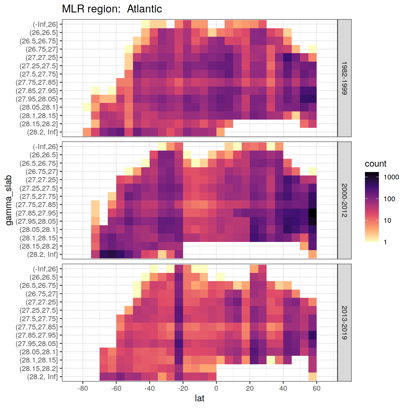
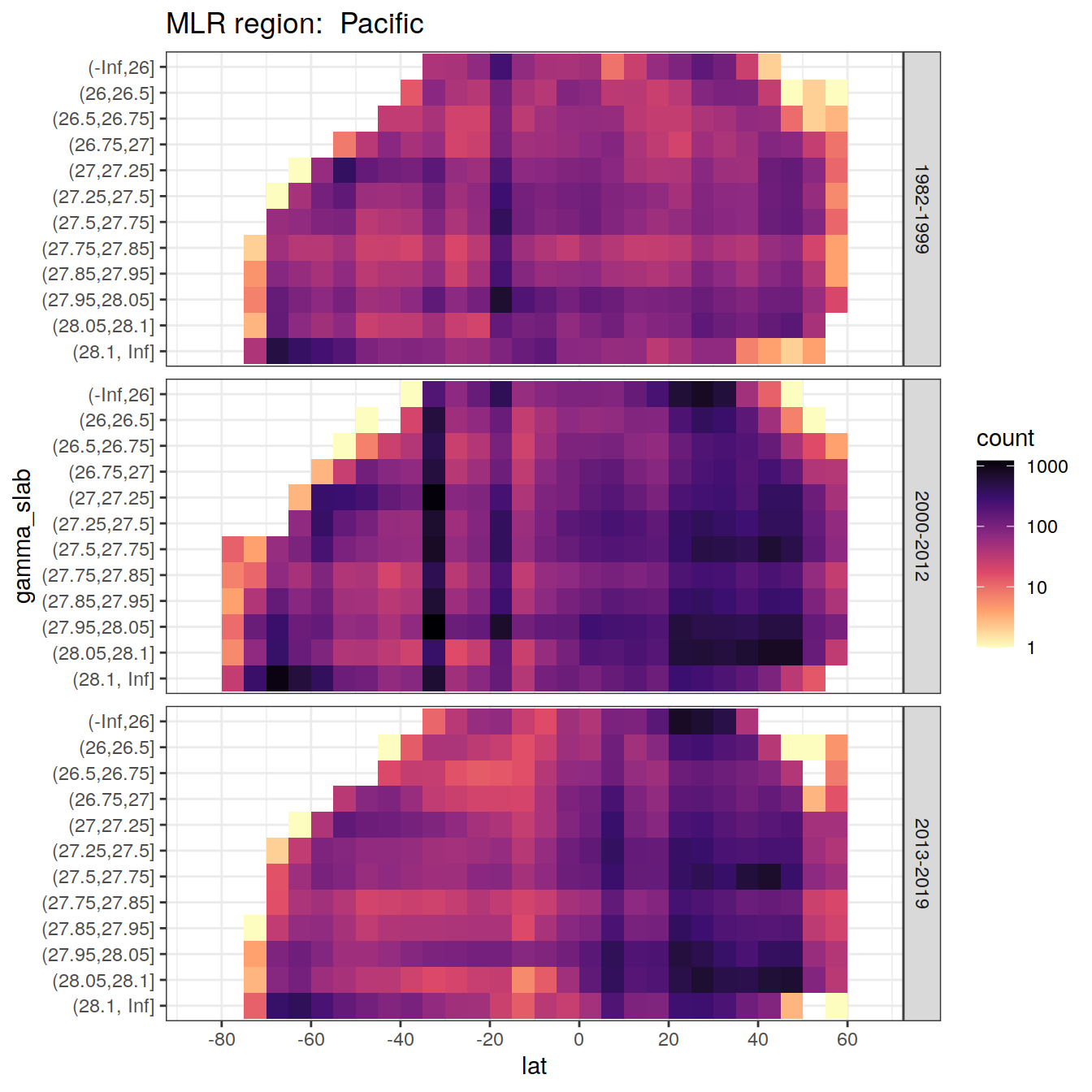
rm(lat_section, GLODAP_cruise, cruises_meridional)

6 Observations coverage

GLODAP <- GLODAP %>% 
  mutate(gamma_slab = factor(gamma_slab), 
         gamma_slab = factor(gamma_slab, levels = rev(levels(gamma_slab))))

for (i_basin in unique(GLODAP$basin)) {
  # i_basin <- unique(GLODAP$basin)[3]
  
  print(
    GLODAP %>%
      filter(basin == i_basin) %>%
      ggplot(aes(lat, gamma_slab)) +
      geom_bin2d(binwidth = 5) +
      scale_fill_viridis_c(
        option = "magma",
        direction = -1,
        trans = "log10"
      ) +
      scale_x_continuous(breaks = seq(-100, 100, 20),
                         limits = c(params_global$lat_min,
                                    params_global$lat_max)) +
      facet_grid(era ~ .) +
      labs(title = paste("MLR region: ", i_basin))
  )
  
}

Version	Author	Date
984697e	jens-daniel-mueller	2020-12-12
3ebff89	jens-daniel-mueller	2020-12-12
7d82772	jens-daniel-mueller	2020-12-11

Version	Author	Date
984697e	jens-daniel-mueller	2020-12-12
3ebff89	jens-daniel-mueller	2020-12-12
7d82772	jens-daniel-mueller	2020-12-11

Version	Author	Date
984697e	jens-daniel-mueller	2020-12-12
3ebff89	jens-daniel-mueller	2020-12-12
7d82772	jens-daniel-mueller	2020-12-11

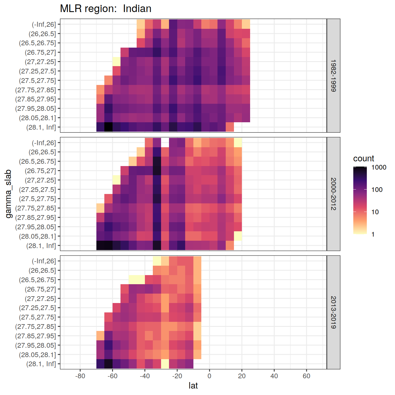
6.1 Histograms

GLODAP_vars <- GLODAP %>% 
  select(cstar_tref,
         sal,
         temp,
         oxygen,
         aou,
         silicate,
         phosphate,
         phosphate_star)

GLODAP_vars_long <- GLODAP_vars %>% 
  pivot_longer(cstar_tref:phosphate_star, names_to = "variable", values_to = "value")

GLODAP_vars_long %>% 
  ggplot(aes(value)) +
  geom_histogram() +
  facet_wrap(~ variable,
             ncol = 2,
             scales = "free")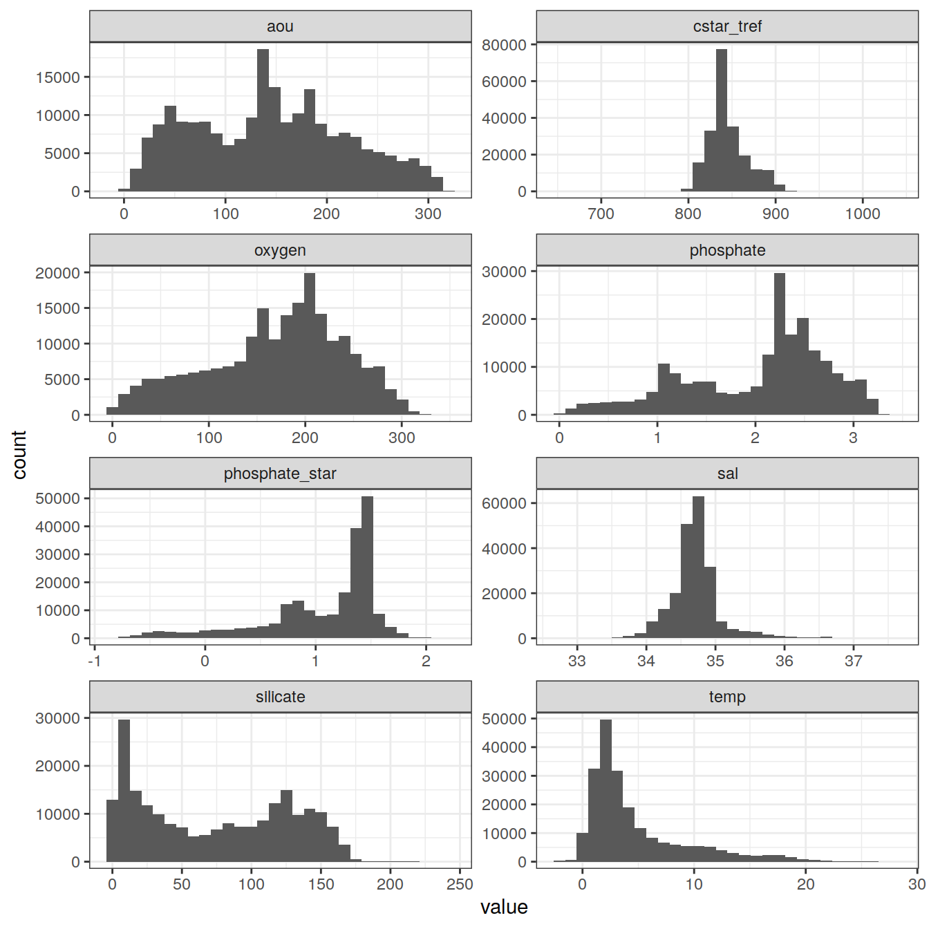

Version	Author	Date
3ebff89	jens-daniel-mueller	2020-12-12
7d82772	jens-daniel-mueller	2020-12-11
7788175	jens-daniel-mueller	2020-12-09

rm(GLODAP_vars, GLODAP_vars_long)

7 Individual cruise sections

Zonal and meridional section plots are produce for each cruise individually and can be downloaded here.

if (params_local$plot_all_figures == "y") {

cruises <- GLODAP %>% 
  group_by(cruise) %>% 
  summarise(date_mean = mean(date, na.rm = TRUE),
            n = n()) %>% 
  ungroup() %>% 
  arrange(date_mean)

GLODAP <- full_join(GLODAP, cruises)

n <- 0
for (i_cruise in unique(cruises$cruise)) {

# i_cruise <- unique(cruises$cruise)[1]
# n <- n + 1
# print(n)  
  
GLODAP_cruise <- GLODAP %>%
  filter(cruise == i_cruise) %>% 
  arrange(date)

cruises_cruise <- cruises %>%
  filter(cruise == i_cruise)
  
map_plot <- 
  map +
  geom_point(data = GLODAP_cruise,
             aes(lon, lat, col = date)) +
  scale_color_viridis_c(trans = "date") +
  labs(title = paste("Mean date:", cruises_cruise$date_mean,
                     "| cruise:", cruises_cruise$cruise,
                     "| n(samples):", cruises_cruise$n))


lon_section <- GLODAP_cruise %>%
  ggplot(aes(lon, depth)) +
  scale_y_reverse() +
  scale_fill_viridis_c()

lon_tco2 <- lon_section+
  stat_summary_2d(aes(z=tco2))

lon_talk <- lon_section+
  stat_summary_2d(aes(z=talk))

lon_phosphate <- lon_section+
  stat_summary_2d(aes(z=phosphate))

lon_oxygen <- lon_section+
  stat_summary_2d(aes(z=oxygen))

lon_aou <- lon_section+
  stat_summary_2d(aes(z=aou))

lon_phosphate_star <- lon_section+
  stat_summary_2d(aes(z=phosphate_star))

lon_nitrate <- lon_section+
  stat_summary_2d(aes(z=nitrate))

lon_cstar <- lon_section+
  stat_summary_2d(aes(z=cstar_tref))


lat_section <- GLODAP_cruise %>%
  ggplot(aes(lat, depth)) +
  scale_y_reverse() +
  scale_fill_viridis_c()

lat_tco2 <- lat_section+
  stat_summary_2d(aes(z=tco2))

lat_talk <- lat_section+
  stat_summary_2d(aes(z=talk))

lat_phosphate <- lat_section+
  stat_summary_2d(aes(z=phosphate))

lat_oxygen <- lat_section+
  stat_summary_2d(aes(z=oxygen))

lat_aou <- lat_section+
  stat_summary_2d(aes(z=aou))

lat_phosphate_star <- lat_section+
  stat_summary_2d(aes(z=phosphate_star))

lat_nitrate <- lat_section+
  stat_summary_2d(aes(z=nitrate))

lat_cstar <- lat_section+
  stat_summary_2d(aes(z=cstar_tref))

hist_tco2 <- GLODAP_cruise %>%
  ggplot(aes(tco2)) +
  geom_histogram()

hist_talk <- GLODAP_cruise %>%
  ggplot(aes(talk)) +
  geom_histogram()

hist_phosphate <- GLODAP_cruise %>%
  ggplot(aes(phosphate)) +
  geom_histogram()

hist_oxygen <- GLODAP_cruise %>%
  ggplot(aes(oxygen)) +
  geom_histogram()

hist_aou <- GLODAP_cruise %>%
  ggplot(aes(aou)) +
  geom_histogram()

hist_phosphate_star <- GLODAP_cruise %>%
  ggplot(aes(phosphate_star)) +
  geom_histogram()

hist_nitrate <- GLODAP_cruise %>%
  ggplot(aes(nitrate)) +
  geom_histogram()

hist_cstar <- GLODAP_cruise %>%
  ggplot(aes(cstar_tref)) +
  geom_histogram()

(map_plot /
    ((hist_tco2 / hist_talk / hist_phosphate / hist_cstar) |
       (hist_oxygen / hist_phosphate_star / hist_nitrate / hist_aou)
    )) |
  ((lat_tco2 / lat_talk / lat_phosphate / lat_oxygen / lat_aou / lat_phosphate_star / lat_nitrate / lat_cstar) |
     (lon_tco2 / lon_talk / lon_phosphate / lon_oxygen /  lon_aou /lon_phosphate_star / lon_nitrate / lon_cstar))    

ggsave(
  path = paste(path_version_figures, "Cruise_sections_histograms/", sep = ""),
  filename = paste(
    "Cruise_date",
    cruises_cruise$date_mean,
    "count",
    cruises_cruise$n,
    "cruiseID",
    cruises_cruise$cruise,
    ".png",
    sep = "_"
  ),
width = 20, height = 12)

rm(map_plot,
   lon_section, lat_section,
   lat_tco2, lat_talk, lat_phosphate, lon_tco2, lon_talk, lon_phosphate,
   GLODAP_cruise, cruises_cruise)

}

}

8 Write files

# select relevant columns
GLODAP <- GLODAP %>%
  select(
    year,
    date,
    era,
    basin,
    basin_AIP,
    lat,
    lon,
    depth,
    gamma,
    gamma_slab,
    params_local$MLR_predictors,
    params_local$MLR_target
  )

GLODAP %>% write_csv(paste(
  path_version_data,
  "GLODAPv2.2020_MLR_fitting_ready.csv",
  sep = ""
))

co2_atm_tref %>%  write_csv(paste(path_version_data,
                                  "co2_atm_tref.csv",
                                  sep = ""))

sessionInfo()

R version 4.0.3 (2020-10-10)
Platform: x86_64-pc-linux-gnu (64-bit)
Running under: openSUSE Leap 15.1

Matrix products: default
BLAS:   /usr/local/R-4.0.3/lib64/R/lib/libRblas.so
LAPACK: /usr/local/R-4.0.3/lib64/R/lib/libRlapack.so

locale:
 [1] LC_CTYPE=en_US.UTF-8       LC_NUMERIC=C              
 [3] LC_TIME=en_US.UTF-8        LC_COLLATE=en_US.UTF-8    
 [5] LC_MONETARY=en_US.UTF-8    LC_MESSAGES=en_US.UTF-8   
 [7] LC_PAPER=en_US.UTF-8       LC_NAME=C                 
 [9] LC_ADDRESS=C               LC_TELEPHONE=C            
[11] LC_MEASUREMENT=en_US.UTF-8 LC_IDENTIFICATION=C       

attached base packages:
[1] stats     graphics  grDevices utils     datasets  methods   base     

other attached packages:
 [1] lubridate_1.7.9 marelac_2.1.10  shape_1.4.5     metR_0.9.0     
 [5] scico_1.2.0     patchwork_1.1.0 collapse_1.4.2  forcats_0.5.0  
 [9] stringr_1.4.0   dplyr_1.0.2     purrr_0.3.4     readr_1.4.0    
[13] tidyr_1.1.2     tibble_3.0.4    ggplot2_3.3.2   tidyverse_1.3.0
[17] workflowr_1.6.2

loaded via a namespace (and not attached):
 [1] httr_1.4.2               viridisLite_0.3.0        jsonlite_1.7.1          
 [4] here_0.1                 modelr_0.1.8             assertthat_0.2.1        
 [7] blob_1.2.1               cellranger_1.1.0         yaml_2.2.1              
[10] pillar_1.4.7             backports_1.1.10         lattice_0.20-41         
[13] glue_1.4.2               RcppEigen_0.3.3.7.0      digest_0.6.27           
[16] RColorBrewer_1.1-2       promises_1.1.1           checkmate_2.0.0         
[19] rvest_0.3.6              colorspace_2.0-0         htmltools_0.5.0         
[22] httpuv_1.5.4             Matrix_1.2-18            pkgconfig_2.0.3         
[25] broom_0.7.2              seacarb_3.2.14           haven_2.3.1             
[28] scales_1.1.1             whisker_0.4              later_1.1.0.1           
[31] git2r_0.27.1             farver_2.0.3             generics_0.0.2          
[34] ellipsis_0.3.1           withr_2.3.0              cli_2.2.0               
[37] magrittr_2.0.1           crayon_1.3.4             readxl_1.3.1            
[40] evaluate_0.14            fs_1.5.0                 fansi_0.4.1             
[43] xml2_1.3.2               RcppArmadillo_0.10.1.2.0 oce_1.2-0               
[46] tools_4.0.3              data.table_1.13.2        hms_0.5.3               
[49] lifecycle_0.2.0          munsell_0.5.0            reprex_0.3.0            
[52] gsw_1.0-5                compiler_4.0.3           rlang_0.4.9             
[55] grid_4.0.3               rstudioapi_0.13          labeling_0.4.2          
[58] rmarkdown_2.5            testthat_3.0.0           gtable_0.3.0            
[61] DBI_1.1.0                R6_2.5.0                 knitr_1.30              
[64] rprojroot_2.0.2          stringi_1.5.3            parallel_4.0.3          
[67] Rcpp_1.0.5               vctrs_0.3.5              dbplyr_1.4.4            
[70] tidyselect_1.1.0         xfun_0.18

eMLR - data preparation

Jens Daniel Müller

15 December, 2020

1 Required data

2 PO₄*

2.1 Calculation

3 C*

3.1 Stoichiometric ratios

3.2 Calculation

3.3 Reference year adjustment

3.3.1 Combine GLODAP + Cant

3.3.2 Merge GLODAP + atm. pCO₂

3.3.3 Calculation

3.4 Control plots

4 Selected section plots

5 Isoneutral slabs

6 Observations coverage

6.1 Histograms

7 Individual cruise sections

8 Write files

eMLR - data preparation

Jens Daniel Müller

15 December, 2020

1 Required data

2 PO4*

2.1 Calculation

3 C*

3.1 Stoichiometric ratios

3.2 Calculation

3.3 Reference year adjustment

3.3.1 Combine GLODAP + Cant

3.3.2 Merge GLODAP + atm. pCO2

3.3.3 Calculation

3.4 Control plots

4 Selected section plots

5 Isoneutral slabs

6 Observations coverage

6.1 Histograms

7 Individual cruise sections

8 Write files

2 PO₄*

3.3.2 Merge GLODAP + atm. pCO₂