Log2021

workflowr

• Summary
• Checks
• Past versions

Last updated: 2021-12-12

Checks: 7 0

Knit directory: GradLog/

This reproducible R Markdown analysis was created with workflowr (version 1.6.2). The Checks tab describes the reproducibility checks that were applied when the results were created. The Past versions tab lists the development history.

---

R Markdown file: up-to-date

Great! Since the R Markdown file has been committed to the Git repository, you know the exact version of the code that produced these results.

Environment: empty

Great job! The global environment was empty. Objects defined in the global environment can affect the analysis in your R Markdown file in unknown ways. For reproduciblity it’s best to always run the code in an empty environment.

Seed: set.seed(20201014)

The command set.seed(20201014) was run prior to running the code in the R Markdown file. Setting a seed ensures that any results that rely on randomness, e.g. subsampling or permutations, are reproducible.

Session information: recorded

Great job! Recording the operating system, R version, and package versions is critical for reproducibility.

Cache: none

Nice! There were no cached chunks for this analysis, so you can be confident that you successfully produced the results during this run.

File paths: relative

Great job! Using relative paths to the files within your workflowr project makes it easier to run your code on other machines.

Repository version: 562e3b2

Great! You are using Git for version control. Tracking code development and connecting the code version to the results is critical for reproducibility.

The results in this page were generated with repository version 562e3b2. See the Past versions tab to see a history of the changes made to the R Markdown and HTML files.

Note that you need to be careful to ensure that all relevant files for the analysis have been committed to Git prior to generating the results (you can use wflow_publish or wflow_git_commit). workflowr only checks the R Markdown file, but you know if there are other scripts or data files that it depends on. Below is the status of the Git repository when the results were generated:

Ignored files:
    Ignored:    .DS_Store
    Ignored:    .Rhistory
    Ignored:    .Rproj.user/
    Ignored:    analysis/.DS_Store
    Ignored:    code/.DS_Store
    Ignored:    data/.DS_Store
    Ignored:    output/.DS_Store

Untracked files:
    Untracked:  analysis/test_log.Rmd

Note that any generated files, e.g. HTML, png, CSS, etc., are not included in this status report because it is ok for generated content to have uncommitted changes.

---

These are the previous versions of the repository in which changes were made to the R Markdown (analysis/Log2021.Rmd) and HTML (docs/Log2021.html) files. If you’ve configured a remote Git repository (see ?wflow_git_remote), click on the hyperlinks in the table below to view the files as they were in that past version.

File	Version	Author	Date	Message
Rmd	562e3b2	llw	2021-12-12	wrong figure name
html	b1ee5d2	llw	2021-12-12	Build site.
Rmd	cdc581e	llw	2021-12-12	update progress
html	5565fdd	liliw-w	2021-11-24	Build site.
Rmd	94a7bb9	liliw-w	2021-11-24	add notes
html	91631c9	liliw-w	2021-11-15	Build site.
Rmd	c50e156	liliw-w	2021-11-15	update log
html	82ed164	liliw-w	2021-09-07	Build site.
Rmd	b776926	liliw-w	2021-09-07	Add Sep 07
html	671dc18	liliw-w	2021-09-02	Build site.
Rmd	60d26b9	liliw-w	2021-09-02	Minor edits
html	88f3dab	liliw-w	2021-09-02	Build site.
Rmd	8706282	liliw-w	2021-09-02	Minor edits
html	90ef72c	liliw-w	2021-09-02	Build site.
Rmd	786b185	liliw-w	2021-09-02	Keep cross mappable genes in the filtering step
html	52d05f0	liliw-w	2021-08-17	Build site.
Rmd	1c75f6f	liliw-w	2021-08-17	wflow_publish("analysis/Log2021.Rmd")
html	6dac5dc	liliw-w	2021-07-08	Build site.
Rmd	6edd0eb	liliw-w	2021-07-08	Add July 06
html	0894fed	liliw-w	2021-07-08	Update figures location
Rmd	9275134	liliw-w	2021-07-08	Move figures for Log2021 to asset folder
html	331721b	liliw-w	2021-07-08	Build site.
Rmd	8bef12c	liliw-w	2021-07-08	Add July 08
html	f6c37ba	liliw-w	2021-06-29	Build site.
Rmd	1b79abb	liliw-w	2021-06-29	Add ‘estimate eQTLGen sigma by indepdent null eQTLGen zscores’
html	15631a8	liliw-w	2021-06-25	Build site.
Rmd	bdc8aec	liliw-w	2021-06-25	minor edits
html	ea89d4f	liliw-w	2021-06-25	Build site.
Rmd	0f60720	liliw-w	2021-06-25	Replication of eQTLGen results in trans-PCO of eQTLGen summary stats
html	25a87c0	liliw-w	2021-06-14	Build site.
Rmd	4fc3dff	liliw-w	2021-06-14	Add eQTLGen’s pvalues QQplot
html	7ca8ec5	liliw-w	2021-06-11	Build site.
Rmd	170be38	liliw-w	2021-06-11	revise ‘comparison with univariate’
html	8ab02f2	liliw-w	2021-06-10	Build site.
Rmd	52166c0	liliw-w	2021-06-10	update Snakemake file with python lines
html	04c44fc	liliw-w	2021-05-26	Build site.
Rmd	1f02e91	liliw-w	2021-05-26	edits
html	096ef88	liliw-w	2021-05-24	Build site.
Rmd	f509189	liliw-w	2021-05-24	edit
html	94425ca	liliw-w	2021-05-24	Build site.
Rmd	d7396a4	liliw-w	2021-05-24	Add ‘Are trans-eQTLs cis-eQTLs?’
html	c54b15b	Lili Wang	2021-03-08	Build site.
Rmd	93bcb5b	Lili Wang	2021-03-08	wflow_publish("analysis/Log2021.Rmd")
html	c884100	Lili Wang	2021-03-01	Build site.
Rmd	da50130	Lili Wang	2021-03-01	wflow_publish("analysis/Log2021.Rmd")
html	40088b2	Lili Wang	2021-02-23	Build site.
Rmd	cbbe319	Lili Wang	2021-02-23	wflow_publish(c("analysis/Log2021.Rmd", "docs/power.lambda0.1.png",
html	85072fc	Lili Wang	2021-02-16	Build site.
Rmd	8960692	Lili Wang	2021-02-16	Update simulation.
html	5f143be	Lili Wang	2021-02-06	Build site.
Rmd	912acee	Lili Wang	2021-02-06	wflow_publish(c("analysis/Log2021.Rmd", "docs/N.png", "docs/caus.png",
html	e15b1db	Lili Wang	2021-02-06	Build site.
Rmd	74c629e	Lili Wang	2021-02-06	wflow_publish(c("analysis/Log2021.Rmd", "docs/power.png", "docs/Muscle_Skeleta.p.funcExplorer.png"))
html	86b2e82	Lili Wang	2021-02-02	Build site.
Rmd	0b5d8d3	Lili Wang	2021-02-02	wflow_publish(c("analysis/Log2021.Rmd", "docs/modules.png", "docs/Muscle_Skeleta.p.WGCNA.png",
html	bb3c016	Lili Wang	2021-01-30	Build site.
html	83d3f1d	Lili Wang	2021-01-30	Build site.
Rmd	3017262	Lili Wang	2021-01-30	wflow_publish(c("analysis/Log2021.Rmd", "data/signals.all.txt",
html	a753e96	Lili Wang	2021-01-26	Build site.
Rmd	b7111b2	Lili Wang	2021-01-26	wflow_publish(c("analysis/Log2021.Rmd", "docs/signalsv.s.FDR.png"))
html	1b48368	Lili Wang	2021-01-26	Build site.
Rmd	9526e7a	Lili Wang	2021-01-26	wflow_publish(c("analysis/Log2021.Rmd", "docs/signalsv.s.FDR.png"))
html	9b6da5c	Lili Wang	2021-01-26	Build site.
Rmd	16f7005	Lili Wang	2021-01-26	wflow_publish(c("analysis/Log2021.Rmd", "data/signals.all.txt"))
html	82152fd	Lili Wang	2021-01-19	Build site.
html	a364419	Lili Wang	2021-01-19	Build site.
Rmd	b8815e3	Lili Wang	2021-01-19	docs/nCross.png
html	0611c35	Lili Wang	2021-01-19	Build site.
Rmd	11c79eb	Lili Wang	2021-01-19	Add simulation.
html	51465ae	Lili Wang	2021-01-17	Build site.
Rmd	cc5fc28	Lili Wang	2021-01-17	wflow_publish("analysis/Log2021.Rmd")
html	1f9d60f	Lili Wang	2021-01-17	Build site.
Rmd	b4ce27b	Lili Wang	2021-01-17	Update GTEx.
html	51b1a4c	Lili Wang	2021-01-04	Build site.
Rmd	23d78aa	Lili Wang	2021-01-04	wflow_git_commit(c("analysis/_site.yml", "analysis/index.Rmd",

---

Dec 13

1. Add trait MS to coloc analysis

• Request summary statistic from link.

• Meta analysis from 15 GWASs.

I added coloc results of MS to earlier section.

2. Look at the colocalized regions between trans and immune traits

coloc regions overview

• I specifically looked at the following three traits, as they have a relatively high proportion of coloc regions from earlier section.

disease	#light green regions	#dark green regions	coloc prop
crohn’s disease (cd)	51	20	0.3921569
Inflammaroty bowel disease (ibd)	48	18	0.3750000
Allergy	43	11	0.2558140

*light green regions: regions with lead module-QTL pvalue<1e-8.

*dark green regions: coloc regions with lead module-QTL pvalue<1e-8.

• What are those dark green regions in specific?

Fig: Colocalized regions summary of crohn’s disease, Inflammaroty bowel disease, Allergic disases. Specifically for dark green regions, i.e. coloc regions with lead module-QTL pvalue<1e-8.

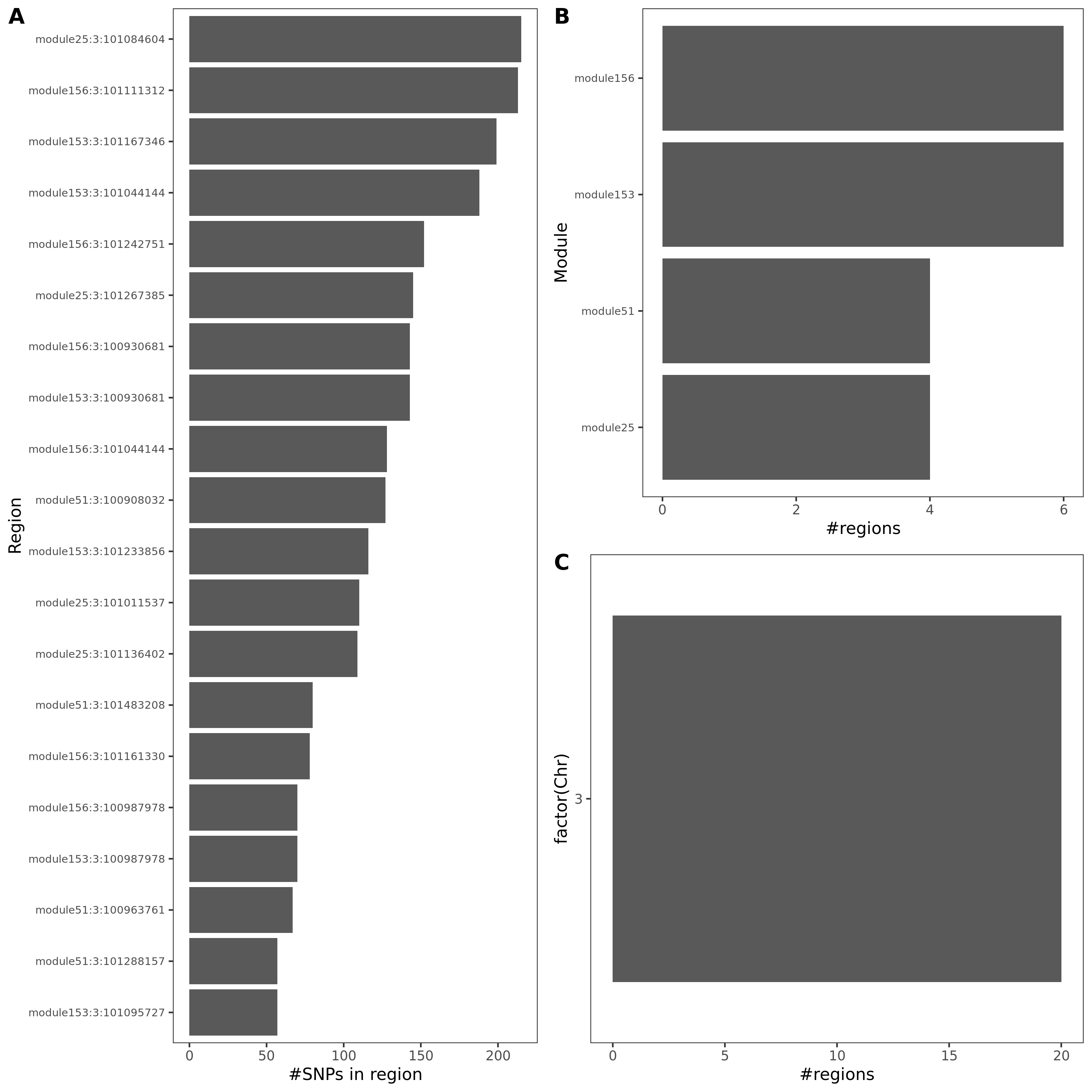
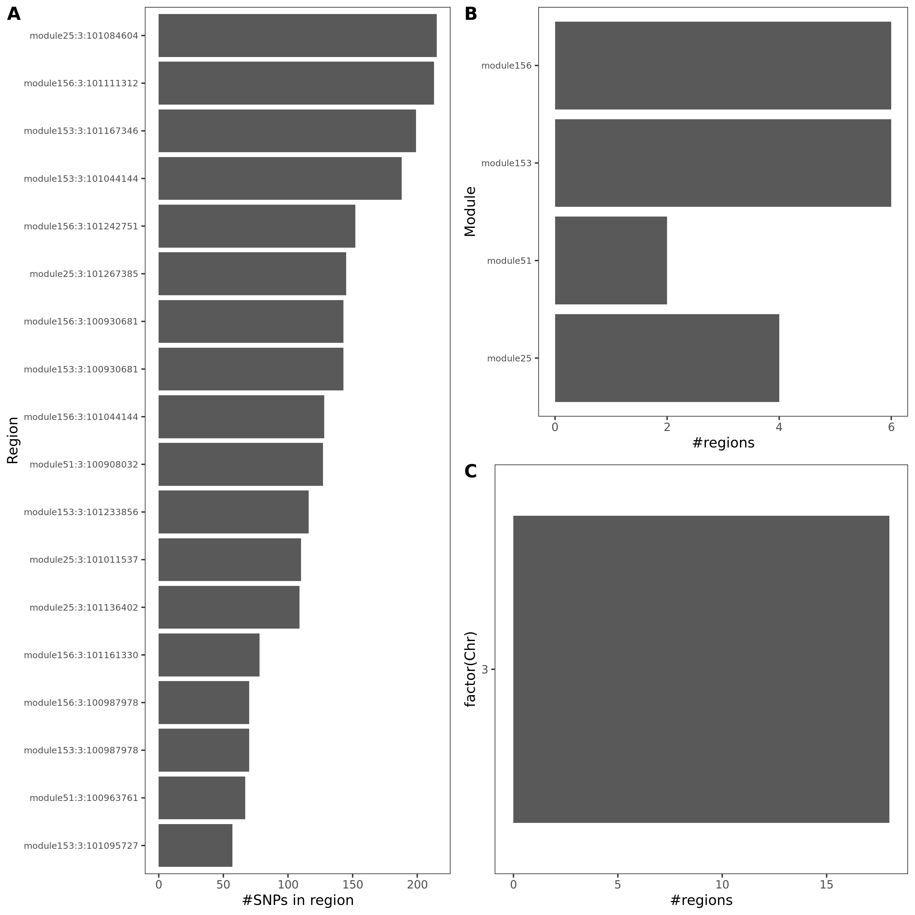
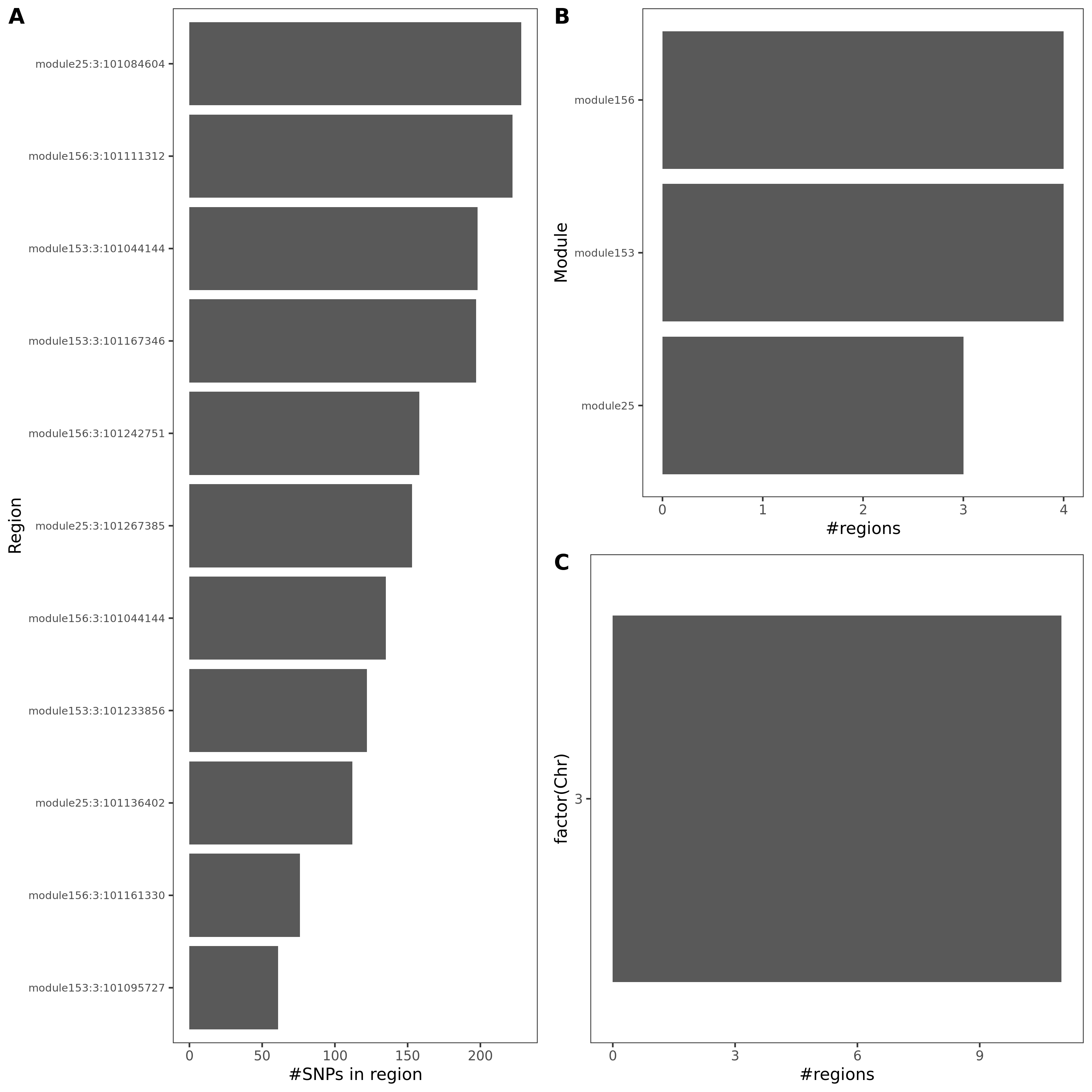
Observations

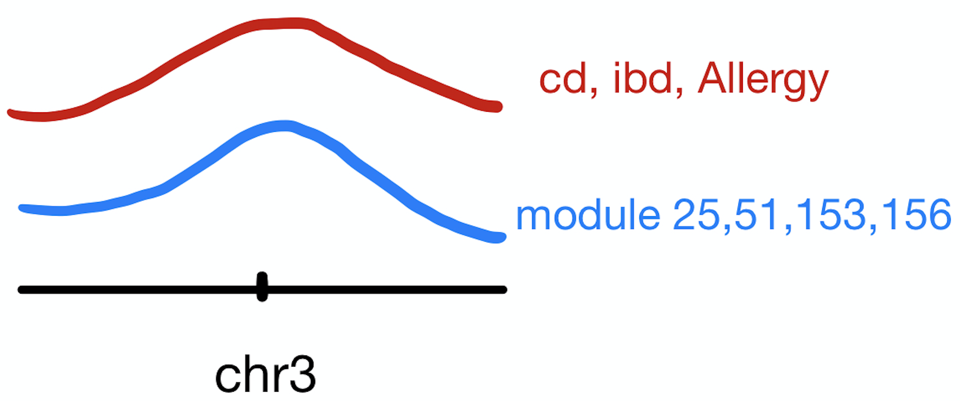
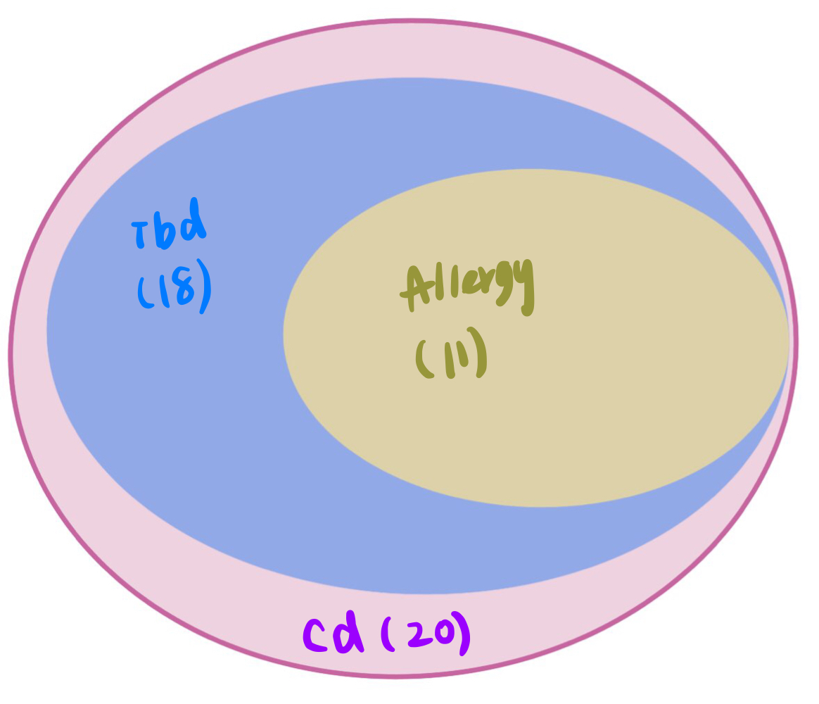
• These three traits share very similar coloc regions.

  See the above venn diagram. The coloc regions of three traits are largely overlapped.

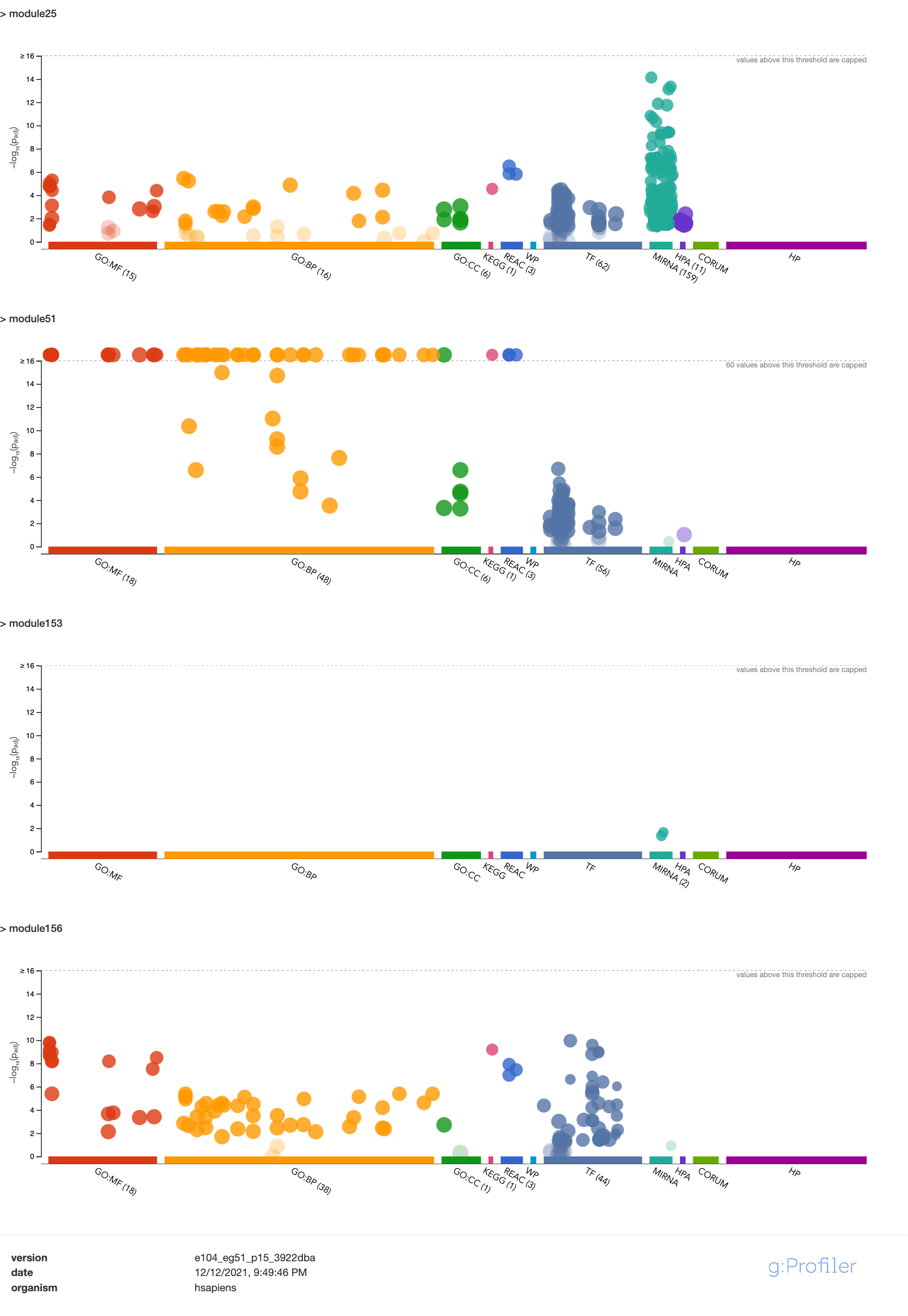
module	#Genes	Enrichment
module25	123	some genes are ZNF* genes
module51	61	almost all genes are ZNF* genes
module153	15
module156	13	12 genes are ZNF* genes

• Module enrichment, relevant to immune?

  • See enrichment results here.

  • See g:profiler enrichment overview.

  • See g:profiler enrichment query file.

  • See David enrichment query file and gene descriptions.

  Question: These four modules contain many zinc finger genes.

• SNP variants

  • cis-genes?

  For the 20 lead SNPs, they are, Intron Variant of gene SENP7, IMPG2, CEP97, Non Coding Transcript Variant/2KB Upstream Variant of gene SENP7, or 500B Downstream Variant of gene FAM172BP.

Nov 29, Dec 06

0. out 130 regions, % of colocalization

I updated it to earlier section -> Observations -> Distribution of coloc regions.

1. Other blood related traits: immune diseases

Traits refer to Paper.

72 GWAS of immune-related and non-immune traits.

We compiled a set of 72 well-powered GWAS, including 14 for autoimmune diseases (11 unique disease types), 36 blood traits, and 22 other traits (Additional File 1: Table S4),

72 publicly available GWAS summary statistics for 11 autoimmune diseases (14 studies).

14 autoimmune diseases overview

See file.

• There are 14 studies (datasets) for 11 immune diseases.

• For two studies (MS, ApD), the summary stat is only available upon request. (Update: we have requested sum stat for MS and added its coloc results here.)

• For one study (sle), the previous dataset is no longer available. So I downloaded the updated version (meta- v.s. EUR-).

• Many studies meta-analyze multiple datasets

  • Use meta sum stat for coloc?
  • Use meta sample sizes of cases and controls?

coloc proportion

The following figure is similar to earlier section, which gives regions and proportions of coloc regions.

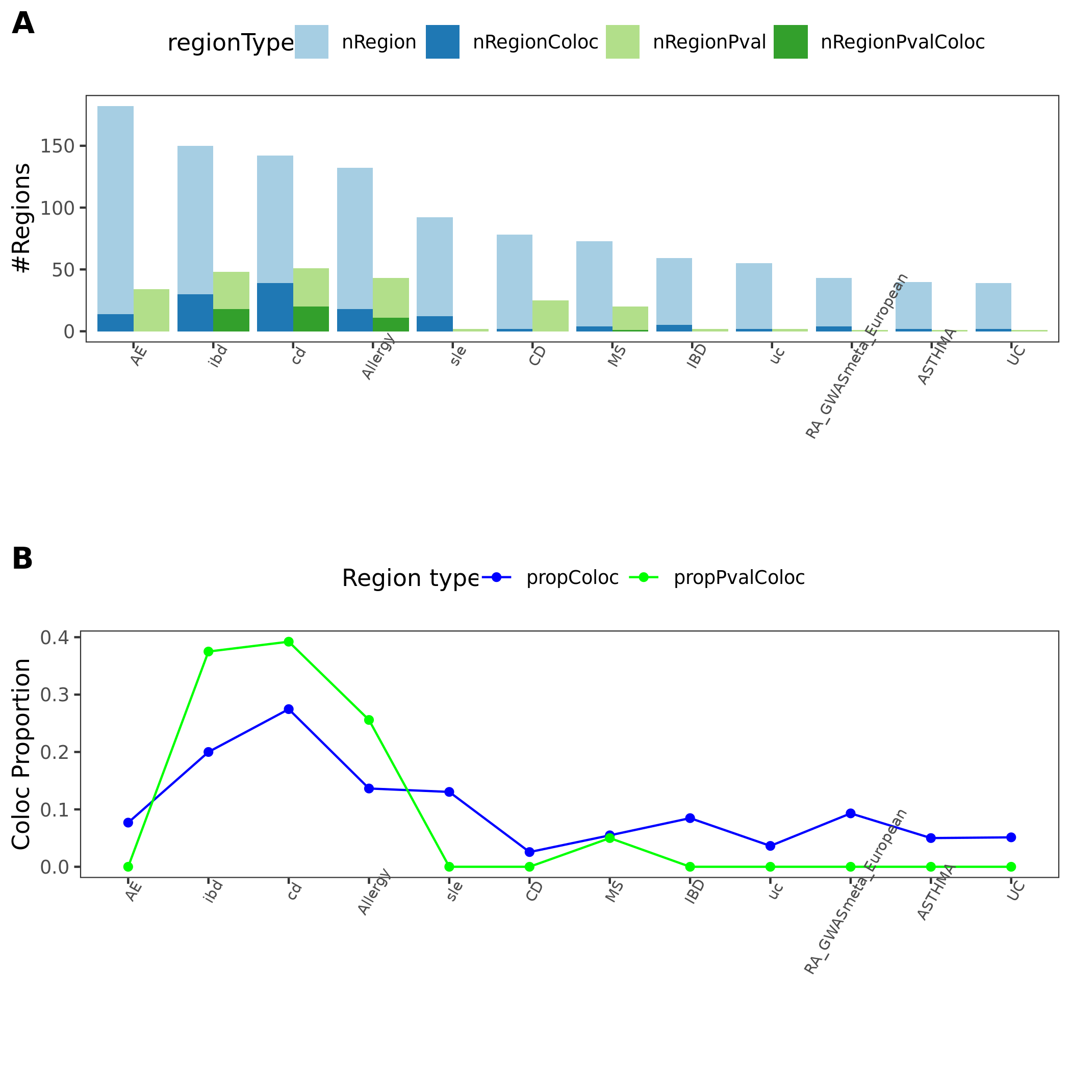
The proportion of colocalized regions for 11 auto-immune diseases.

Past versions of 1129_all.traits.coloc.region.summary.png

Version	Author	Date
69b76c8	llw	2021-12-12

For a specific trait, the coloc regions’ summary and visualization are in folder /scratch/midway2/liliw1/coloc/pmid*_*/plot.

Observations

• These 11 immune diseases generally have less blue regions (GWAS regions with minimum QTL \(p>10^{-5}\)).

• Also less green regions (regions with very small module-QTL pvalues).

• Also lower proportion of coloc regions, out of blue and green regions. 8 diseases have 0 coloc regions.

• Due to meta-analysis? Cell type complexity?

2. MR under assumption of \(\text{var}{\beta}\) (on slack)

Procedure

For MR R package and code tutorial, see earlier section.

Basically, we will need \(\beta\), \(\text{se}({\beta})\) for both module-QTLs and GWAS-QTLs. However, we don’t have estiamted \(\beta\) for module-QTLs. What we have is just \(p\).

Therefore, on slack, assumptions to make TwoSampleMR work,

• (Strong assumption) set \(\beta=z\), \(\text{se}({\beta})=1\).

• (Strong assumption) Since we only have \(p\), we will only have absolute zscores. So one way to deal with this is to assume \(\beta_{SNP-module}\) and \(\beta_{SNP-GWAS}\) have the same sign (+), so that we only consider the consistency of effect magnitude.

• We look at each trans-eQTL region separately, rather than combine all trans-eQTL regions for a module, as what we do here is “like mediation analysis, SNP affect trait through this gene module”, “rather than to infer if the module is causal for the trait, the causality between module and trait”.

Results

Here I take trait 30090 (platelet crit) for an example.

MR result in figure pheno30090.region.mr.png.

Observations

• \(\beta_{SNP-module}\) is much larger than \(\beta_{SNP-GWAS}\).

• Insufficient (1) or only a few (mostly 2, a few 3) independent SNPs (IV) used for MR, as we consider one region each time and the region is quite short (100k).

Nov 23

1. Are the dark green signals eQTLGen signals?

Procedure

• Check those dark green signals (colocalized regions): region lead SNP’s module-QTL \(p<10^{-8}\), \(\text{PP4} > 0.75\), and \(\text{#SNPs in region} \ge 5\).

• eQTLGen SNPs, cis- & trans- signals.

Observations

• trans-

  #all regions for all traits: 551 .
  #unique regions: 105 .
  #unique lead SNPs: 74 .
  Out of 74 unique lead SNPs, 9 are included in eQTLGen trans- SNPs.
  Out of 9 SNPs, 9 are eQTLGen trans- signals.

• cis-

  #all regions for all traits: 551 .
  #unique regions: 105 .
  #unique lead SNPs: 74 .
  Out of 74 unique lead SNPs, 65 are included in eQTLGen cis- SNPs.
  Out of 65 SNPs, 61 are eQTLGen cis- signals.
  

• trans- & cis-

  Out of 74 unique lead SNPs, 65 are included in eQTLGen SNPs.
  Out of 65 SNPs, 63 are eQTLGen cis- or trans- signals.

2. Look at module 15

We wanted to look at module15, because in earlier section, we found that module15 correspond to multiple regions extensively colocalized with multiple ukbb traits, but we didn’t find any enrichment of the genes in module15.

• coloc region & traits

  See file for detailed traits and regions.

The colocalization between the module and traits are from the following regions (marked by lead SNPs):

Region	traits	cis_genes	link_gene	link_snp	note
module15:17:33867678	5	SLFN12L;SLFN14	https://www.ncbi.nlm.nih.gov/gene/100506736;https://www.ncbi.nlm.nih.gov/gene/342618
module15:19:4502201	7	PLIN4	https://www.ncbi.nlm.nih.gov/gene/729359
module15:2:60725451	1
module15:2:8762414	14	ID2	https://www.ncbi.nlm.nih.gov/gene/3398
module15:6:139840693	7	CITED2	https://www.ncbi.nlm.nih.gov/gene/10370	https://www.ncbi.nlm.nih.gov/snp/rs592423?horizontal_tab=true#publications
module15:7:50426097	10	IKZF1	https://www.ncbi.nlm.nih.gov/gene/10320		intron

The coloc traits are from the follwing trait groups, mostly Red blood cells. (bc we have more Red blood cells traits?)

GWAS Group	#traits
Platelets	1
Red blood cells	14
White blood cells	2

• module15

  191 genes. Enrichment in g:profiler

??? genes: number, enrichment in David

3. Look at module 4

We wanted to look at module4, because in earlier section, we found that module4 correspond to multiple regions extensively colocalized with multiple ukbb traits.

• coloc region & traits

  See file for detailed traits and regions.

The colocalization between the module and traits are from the following regions (marked by lead SNPs):

Region	traits	cis_genes	link_gene	link_snp	note
module4:1:248039451	15	OR2W3;TRIM58	https://www.ncbi.nlm.nih.gov/gene/343171;https://www.ncbi.nlm.nih.gov/gene/25893	https://www.ncbi.nlm.nih.gov/snp/rs3811444?horizontal_tab=true#publications	introns
module4:3:56848999	3	ARHGEF3	https://www.ncbi.nlm.nih.gov/gene/50650	https://www.ncbi.nlm.nih.gov/snp/rs6445826?horizontal_tab=true	intron of ARHGEF3
module4:3:56901292	4	ARHGEF3	https://www.ncbi.nlm.nih.gov/gene/50650	https://www.ncbi.nlm.nih.gov/snp/rs6445826?horizontal_tab=true	intron of ARHGEF3
module4:9:99118445	4	SLC35D2	https://www.ncbi.nlm.nih.gov/gene/11046	https://www.ncbi.nlm.nih.gov/snp/rs11794772?horizontal_tab=true	intron

The coloc traits are from the follwing trait groups, mostly Red blood cells

GWAS Group	#traits
Platelets	4
Red blood cells	12
White blood cells	5

4. coloc between cis- and trans- signals

Procedure

• 130 regions, based on module-QTLs. With region lead SNP’s module-QTL \(p<10^{-8}\) and with at least one cis- gene.

• I will test colocalization between module and a gene, if the genes’ 500k flanking region have (>5) overlapped SNPs with the module region.

• Update the region by the overlapped SNPs of both module-QTLs and gene eQTLs.

• Exclude the region if the minimum eQTL \(p>10^{-5}\).

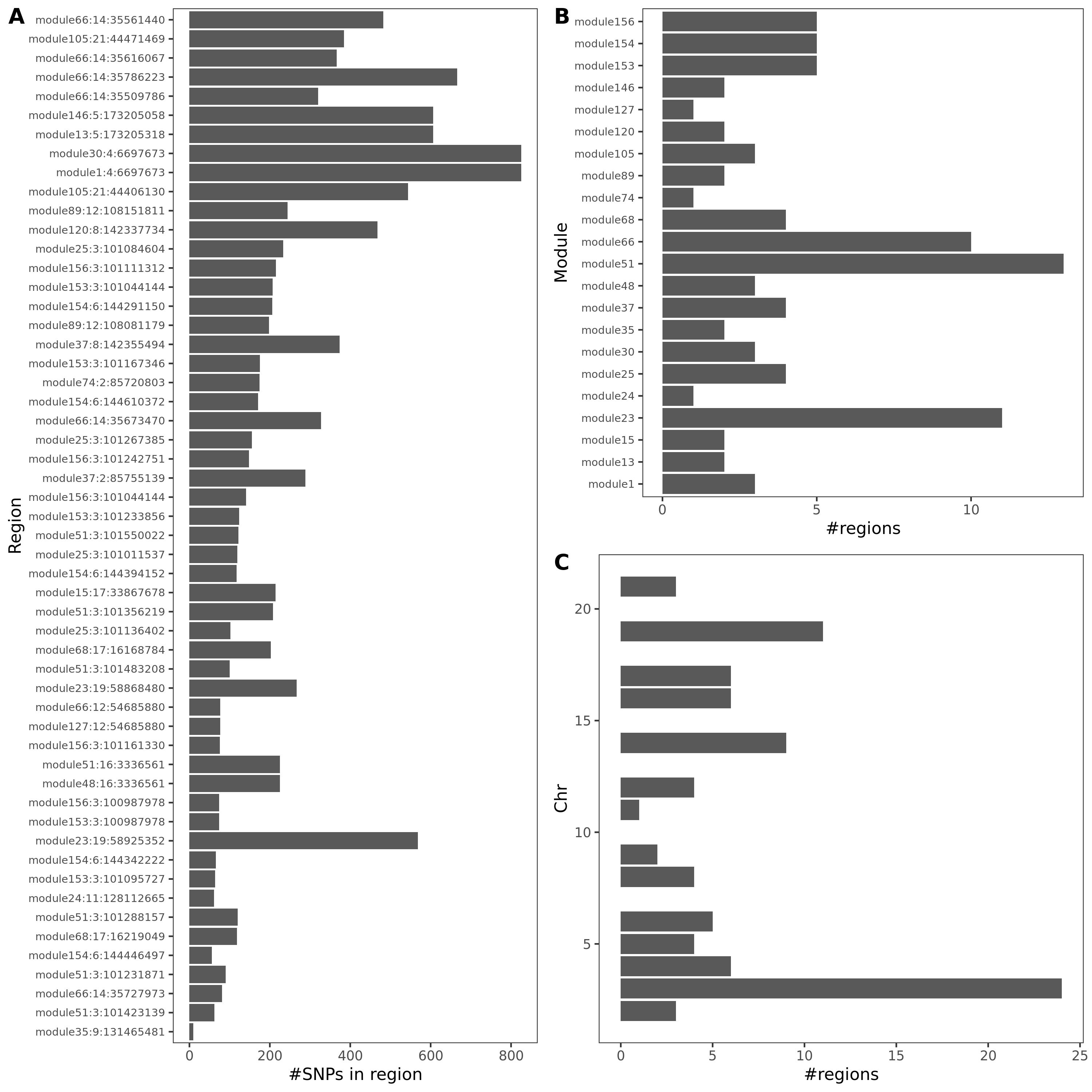
Basics

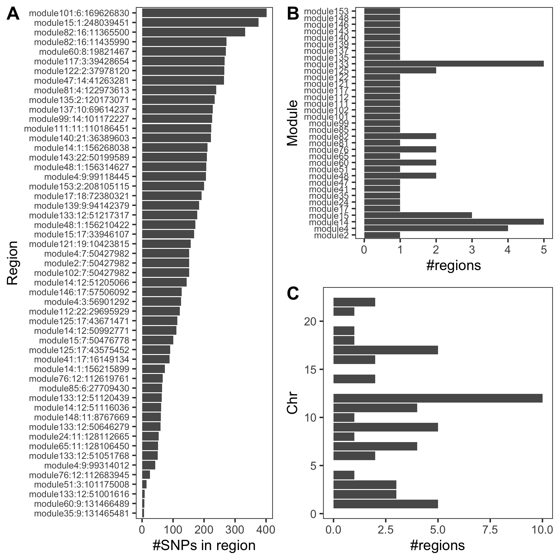
130 regions. With region lead SNP’s module-QTL \(p<10^{-8}\) and with at least one cis- gene.

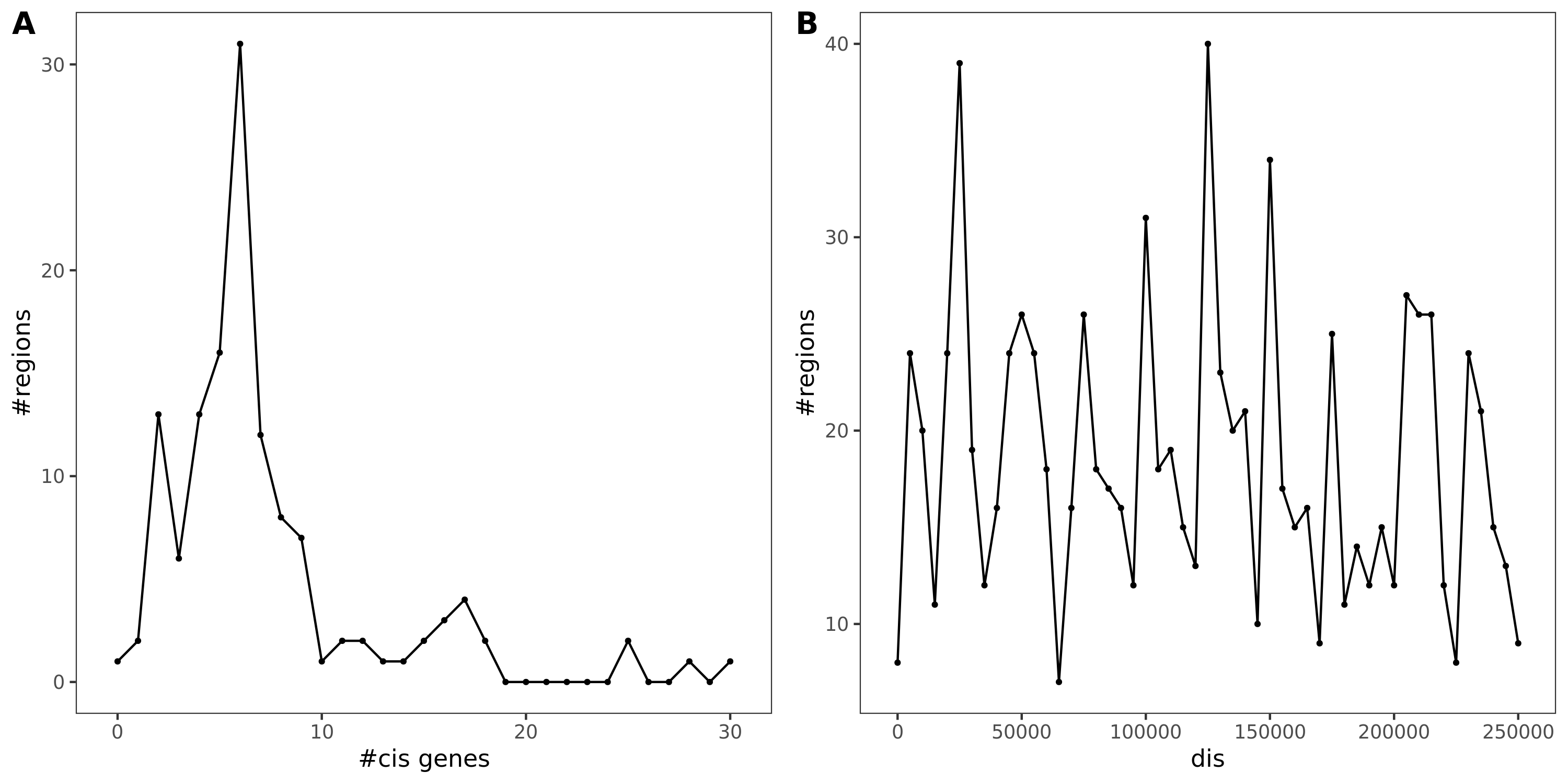
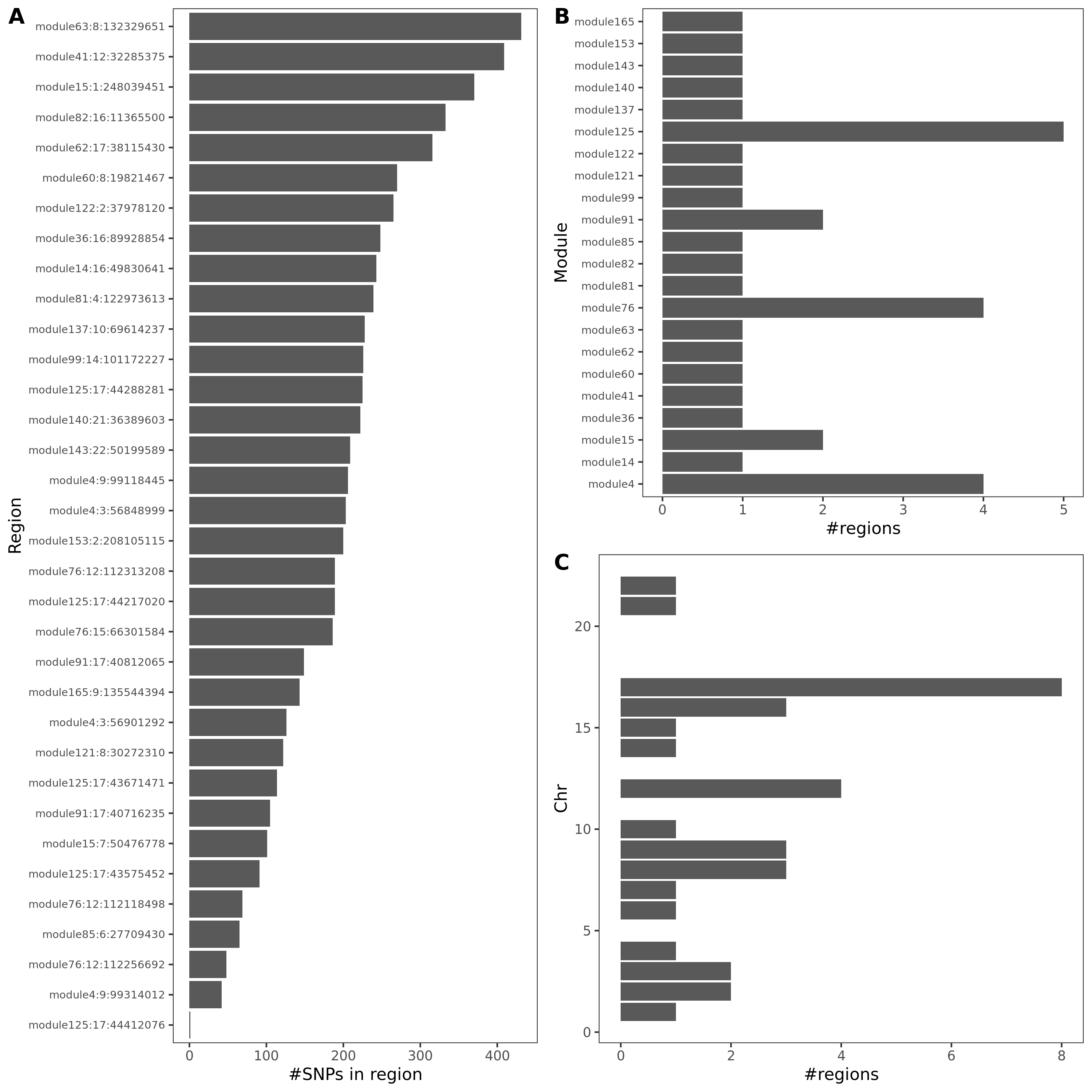
Fig A: region v.s. #cis genes. Fig B: region v.s. dis

Past versions of 1123_region.cis.gene.png

Version	Author	Date
eb8733a	liliw-w	2021-11-24

Observations

• As a result, there are 429 (region, module, gene) sets remained.

• Out of which, 89 regions are colocalized (PP.H4.abf > 0.75).

• Distribution of coloc regions

Past versions of 1123_cis_coloc.region.summary.png

Version	Author	Date
eb8733a	liliw-w	2021-11-24

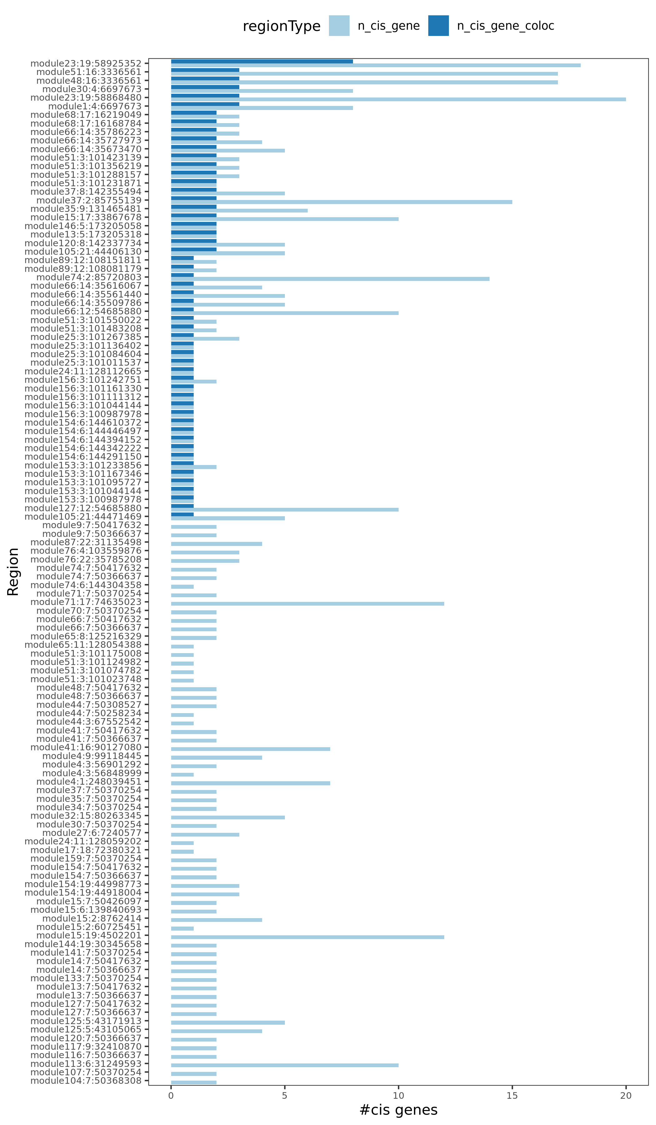
Region v.s. #cis genes. Light blue is for the cis genes near the region. Dark blue is for the colocalized cis genes. There are 120 regions in total, out of which 54 have at least one colocalized cis- gene.

Past versions of 1123_fig_bar_prop_cis.png

Version	Author	Date
eb8733a	liliw-w	2021-11-24

Note: Here there are 120 regions instead of 130 regions, because I excluded the cis- gene regions with \(min(p)>10^{-5}\) before I do the coloc.

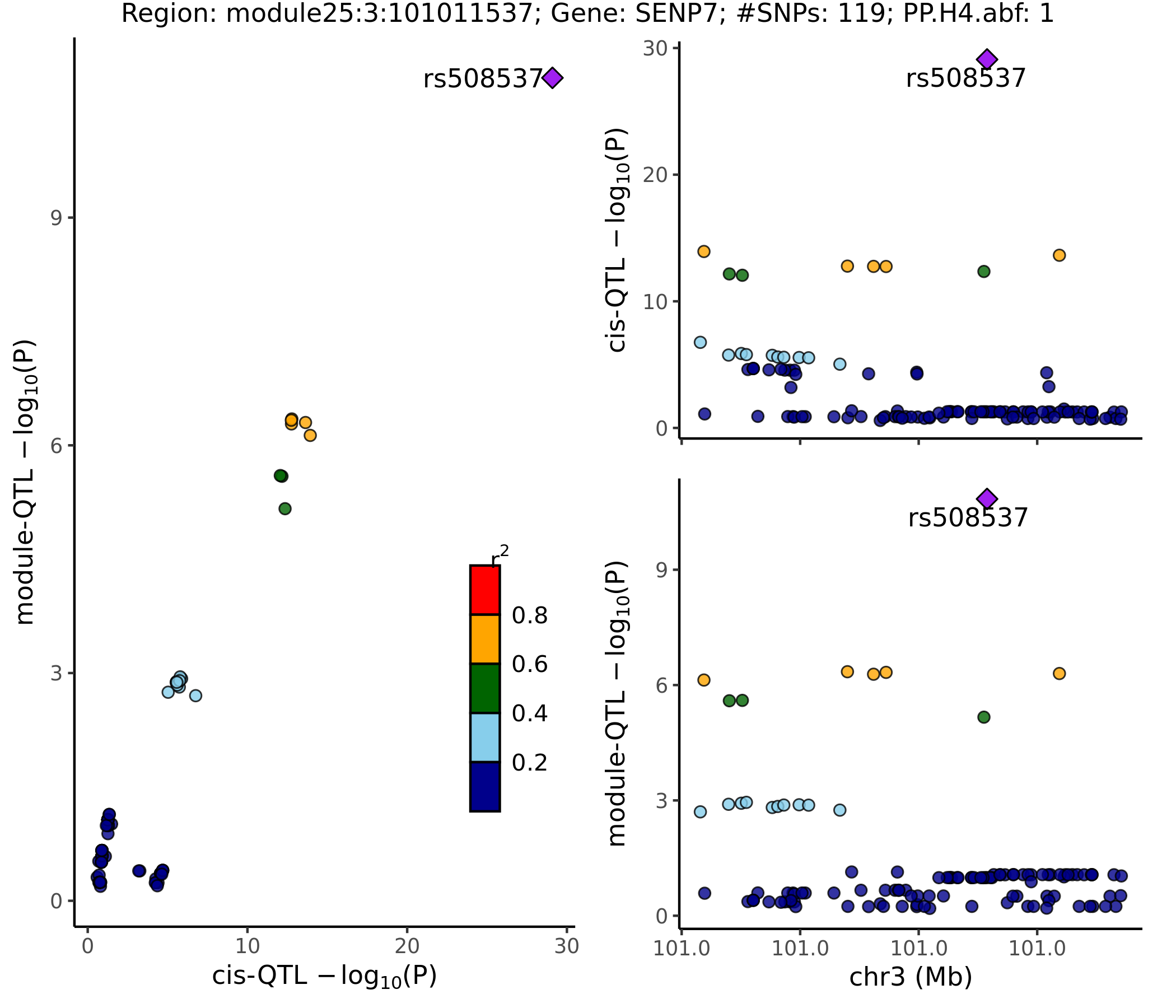
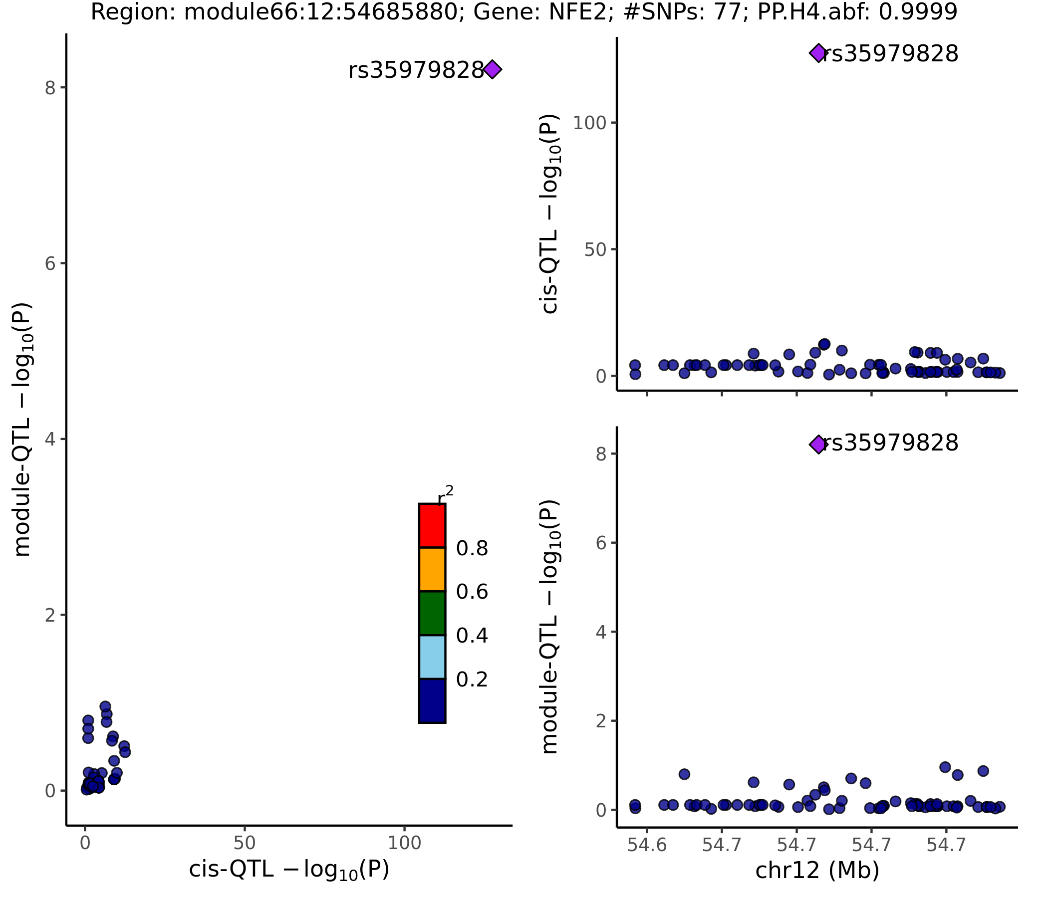
• Colocalized region visualization

Nov 15

1. Proportion of colocalized regions for 29 blood related UKBB traits

Procedure

• Aim: to see how many regions have shared signals for both trait and module. (PP4 > 0.75)

• I consider two types of regions:

  1. One type as stated at last week. Based on module-QTLs and GWAS-QTLs with \(p<10^{-5}\).
  2. Among the above regions, only use regions whose lead SNPs are module-QTLs signals. (Note, here I used the threshold \(p<10^{-8}\), as I don’t have module-signals based on empirical null FDR correction yet.)

• Colocalized regions

  Defined as regions with \(\text{PP4} > 0.75\) and \(\text{#SNPs in region} \ge 5\).

Results

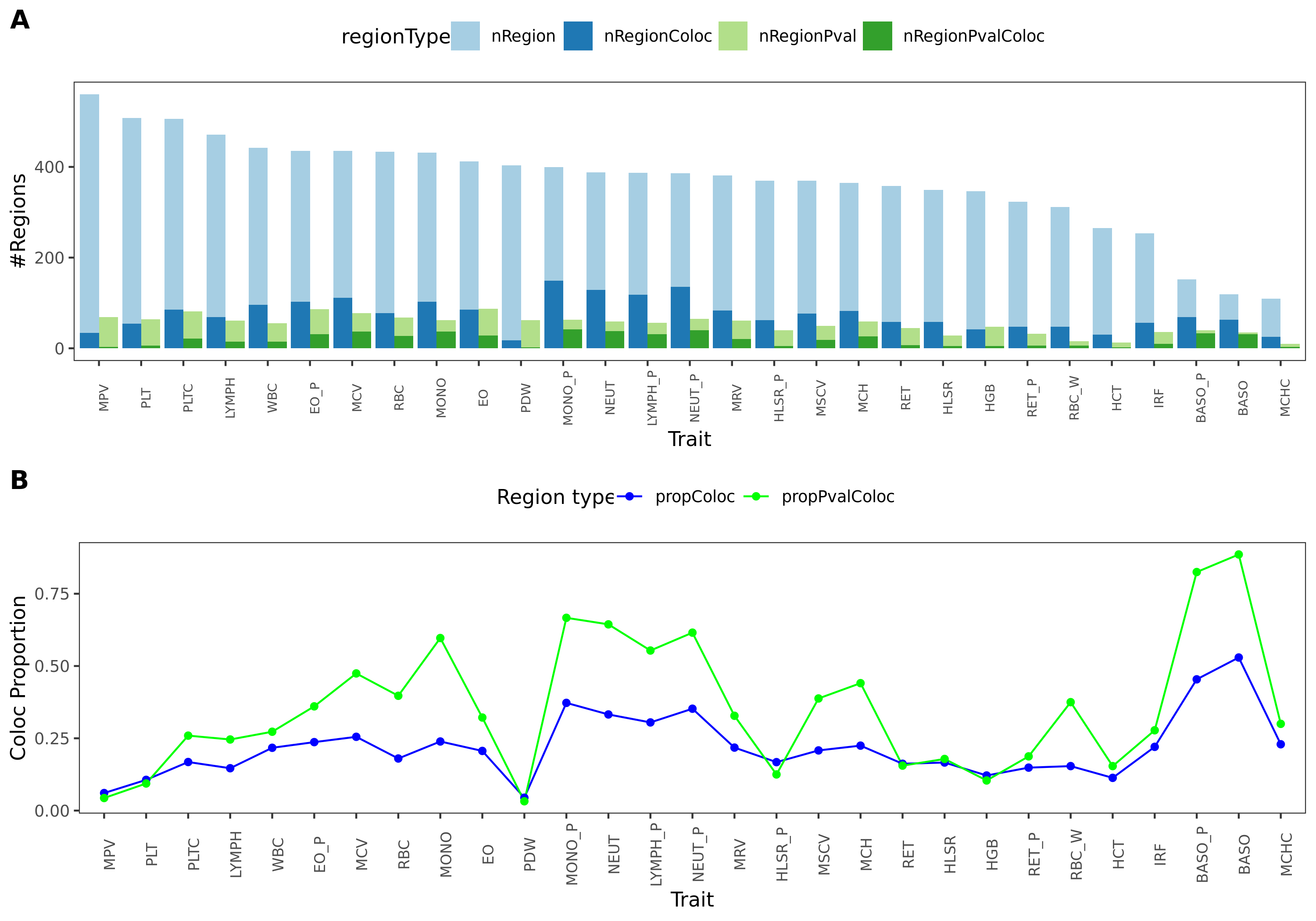
The proportion of colocalized regions for 29 blood-related UKBB traits.

Past versions of 1115_all.traits.coloc.region.summary.png

Version	Author	Date
b27c4e1	liliw-w	2021-11-15

• This figure gives (1) the number of regions at the upper panel, (2) proportion of colocalized regions at the lower panel.

• Blue is for the frist type of regions. Green is for the second type of reigons, based on module-QTL signals.

• Dark color is for the colocalized regions, while light color is for the base regions.

2. Enrichment of colocalized regions

Procedure

• colocalized regions: region lead SNP’s module-QTL \(p<10^{-8}\), \(\text{PP4} > 0.75\), and \(\text{#SNPs in region} \ge 5\).

• Look at the enrichment of these colocalized regions, and the relationship with the corresponding trait.

Results

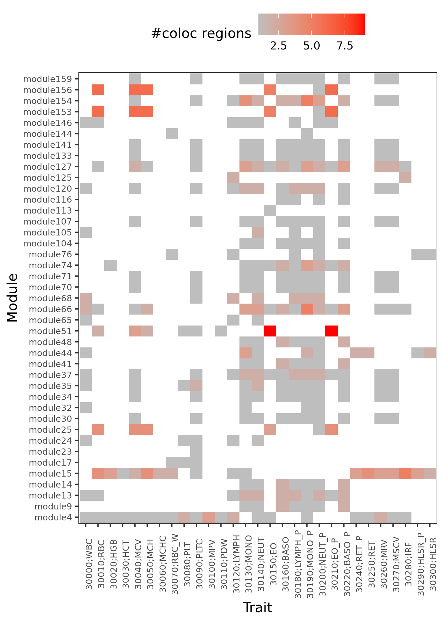
traits v.s. module v.s. coloc region

Past versions of 1115_traits.module.coloc.region.png

Version	Author	Date
b27c4e1	liliw-w	2021-11-15

• The above figure shows, what are the modules that have colocalized regions with a trait.

• Similar traits should have similar colocalized module patterns.

Phenocode	Trait Abbreviation	Trait	g:Profiler
30000	WBC	White blood cell count	https://biit.cs.ut.ee/gplink/l/jWgRmfj9SM
30140	NEUT	Neutrophill count	https://biit.cs.ut.ee/gplink/l/Hs8Nsb99QV
30200	NEUT_P	Neutrophill percentage	https://biit.cs.ut.ee/gplink/l/NKfAXoO9Sp
30300	HLSR	High light scatter reticulocyte count	https://biit.cs.ut.ee/gplink/l/VJWuuEEzTF

• This table gives the enrichment of the module genes for each trait.

• “module4” enriched in platelet activation. Many traits among these 29 blood-related traits are colocalized with “module4”.

• Although “module15” is extensively colocalized with many traits, it’s not enriched in any pathway.

3. Mendelian Randomization (MR) among SNPs, module, trait

• Use R package TwoSampleMR.

• Problem: no \(\beta, \text{se}(\beta)\) for module as exposure. Exposure file requirements see here.

• Use SMR? No. As SMR is also \(\beta, \text{se}(\beta)\) based. In addition to that, it only uses one SNP as instrument variable.

  • SMR only uses one SNP as instrument variable. “top associated cis-eQTL”.
  • Distinguishing pleiotropy from linkage; test for pleiotropic association.

• How people do MR? Paper-Yanyu

  1. the instrument variants were selected using LD clumping function (ld_clump) in the R package ieugwasr

We used the EUR super-population in 1000 Genomes data (1000 Genomes Project Consortium, 2015) as the LD reference panel and the data was downloaded from http://fileserve.mrcieu.ac.uk/ld/1kg.v3.tgz. The LD clumping parameters were clump_kb = 10000 and clump_r2 = 0.001. The p-value parameter (clump_p) in the LD clumping was 10−5 for IDP GWAS and 5 × 10−8 for phenotype GWAS, which gave approximately independent and significant variant instruments.

2. The MR analysis was performed using the R package TwoSampleMR

reported the MR results using three MR methods: i) inverse variance weighted MR (Burgess et al., 2013); ii) median-based estimator: weighted median (Bowden et al., 2016); iii) MR Egger analysis (Bowden et al., 2015), which corresponds to mr_ivw, mr_weighted_median, and mr_egger_regression in TwoSampleMR.

3. further reported a meta-analyzed p-value summarizing the results of the three MR tests being performed

The meta-analysis is based on an extension of ACAT method (Liu et al., 2019) that takes into account the direction of the effects.

Nov 08

Some statistics

• Out of 6,203,169 SNPs in DGN, 6,133,791 (~98.88%) are also included in UKBB GWAS SNPs, 69,378 snps are missed.

• Among 6,133,791 overlapped SNPs, 5,753,809 (~93.81%) are high_quality variants.

coloc procedure

• To do coloc, I compare the pvalues of SNPs within a specific region from each module in DGN and a GWAS trait.

  • For DGN, I use the pvalues from the procedure where I didn’t filter genes based on mappability. There are 166 modules.

  • For GWAS, I use the summary statistics of EUR population.

• Define Regions

  I define coloc regions based on DGN pvalues. For a module, I first sort the pvalues and pick the SNP with the smallest p. Then collect the SNPs in flanking regions within 100kb. These SNPs consist of the first region. Then use the second smallest p and define a second region out of the remaining SNPs. I only consider the regions within which at least one SNP has ** \(p<1e-5\) **.

• SNP filtering

  Based on the above preliminary regions, I updated the regions based on the following criterias:

  • Remove SNPs not included in GWAS.
  • Remove SNPs without rsid.
  • Remove SNPs with low_confidence, no high_quality.
  • Remove duplicated SNPs.
  • Remove the regions within which all SNPs have GWAS ** \(p>1e-5\) **.
  • Remove SNPs with GWAS \(se(\beta)=0\), for coloc purpose.

• Do coloc

  • Use the simple coloc, coloc.abf.
  • A region with PP4 > 0.75 is defined as being colocalized.

Results

1. Trait v.s. #regions v.s. #coloc regions

UKBB trait id	Trait	#regions	#coloc regions
30080	Platelet count	508	54
30090	Platelet crit	506	85
30100	Mean platelet volume	560	35

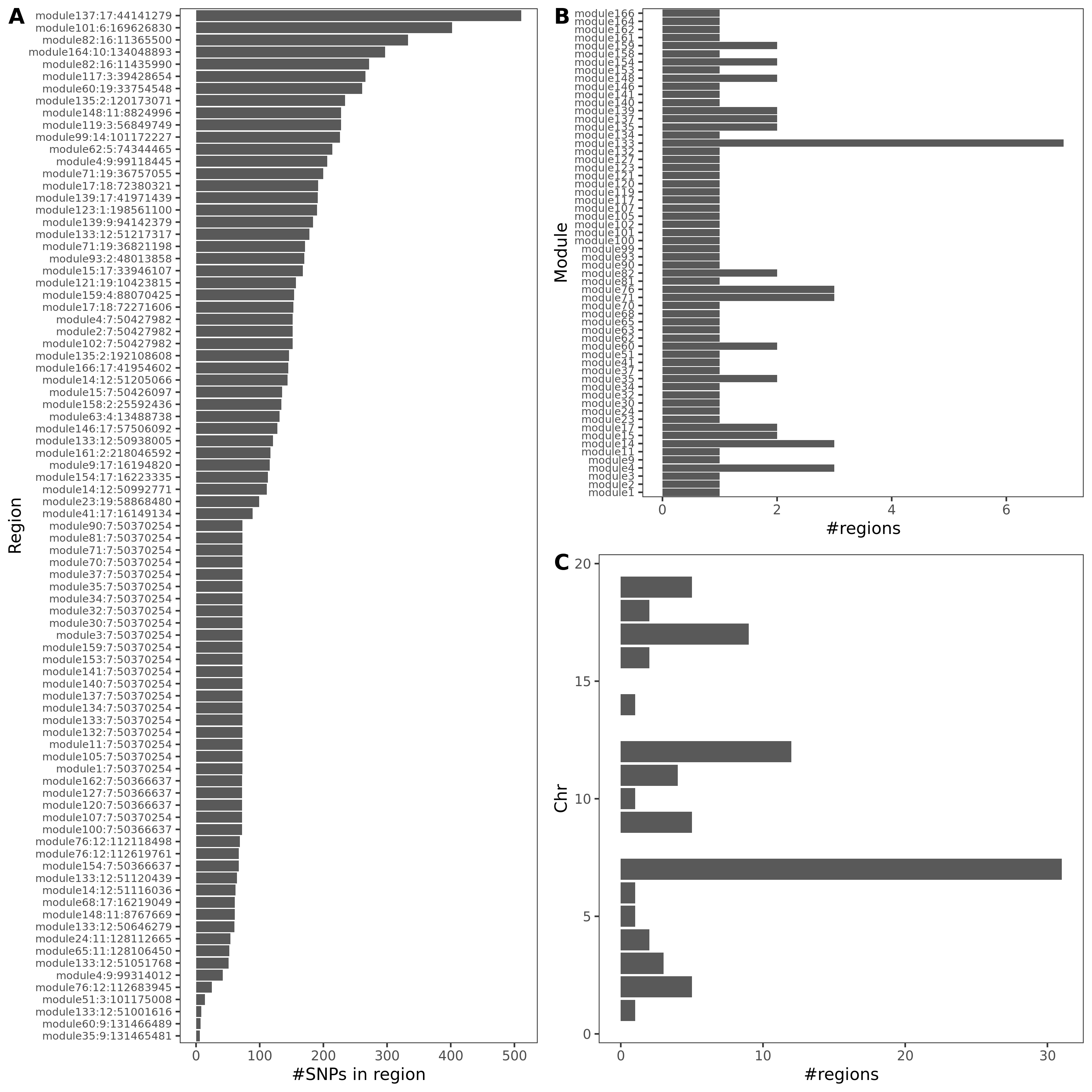
2. #SNPs in colocalized regions

An example of colocalized region visualization. Trait Platelet count.

Past versions of 1108_coloc.region.summary.png

Version	Author	Date
b27c4e1	liliw-w	2021-11-15

An example of colocalized region visualization. Trait Platelet crit

Past versions of 1108_pheno30090.coloc.region.summary.png

Version	Author	Date
b27c4e1	liliw-w	2021-11-15

An example of colocalized region visualization. Trait Mean platelet volume

Past versions of 1108_pheno30100.coloc.region.summary.png

Version	Author	Date
b27c4e1	liliw-w	2021-11-15

3. Colocalized region visualization by locuscomparer

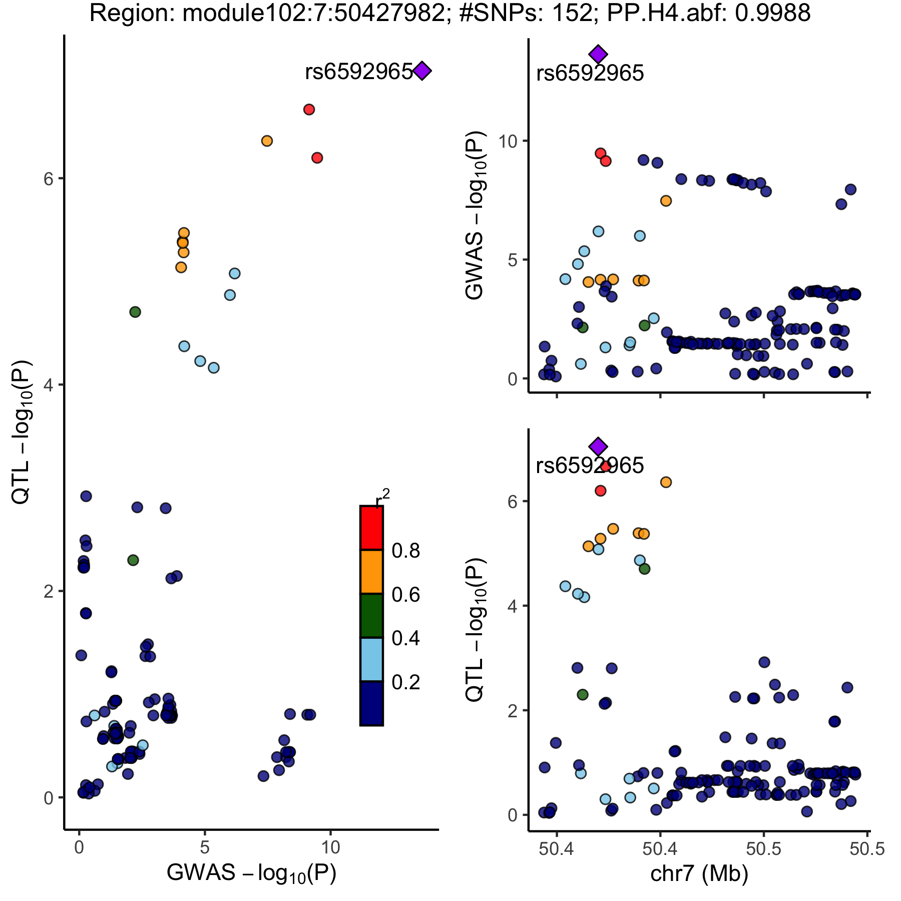
An example of colocalized region visualization.

Past versions of 1108_pheno30080.module102:7:50427982.reg.coloc.png

Version	Author	Date
b27c4e1	liliw-w	2021-11-15

4. 29 UKBB blood traits

For our study, we examined 29 blood trait GWASs in the UK Biobank, including traits from platelets, red blood cells, white blood cells and reticulocytes (Table S1A).

Nov 01

Colocalization

enloc

Paper:

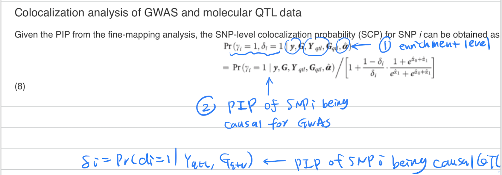
enloc equation

Past versions of 1101_enloc_theory.png

Version	Author	Date
b27c4e1	liliw-w	2021-11-15

Code tutorial:

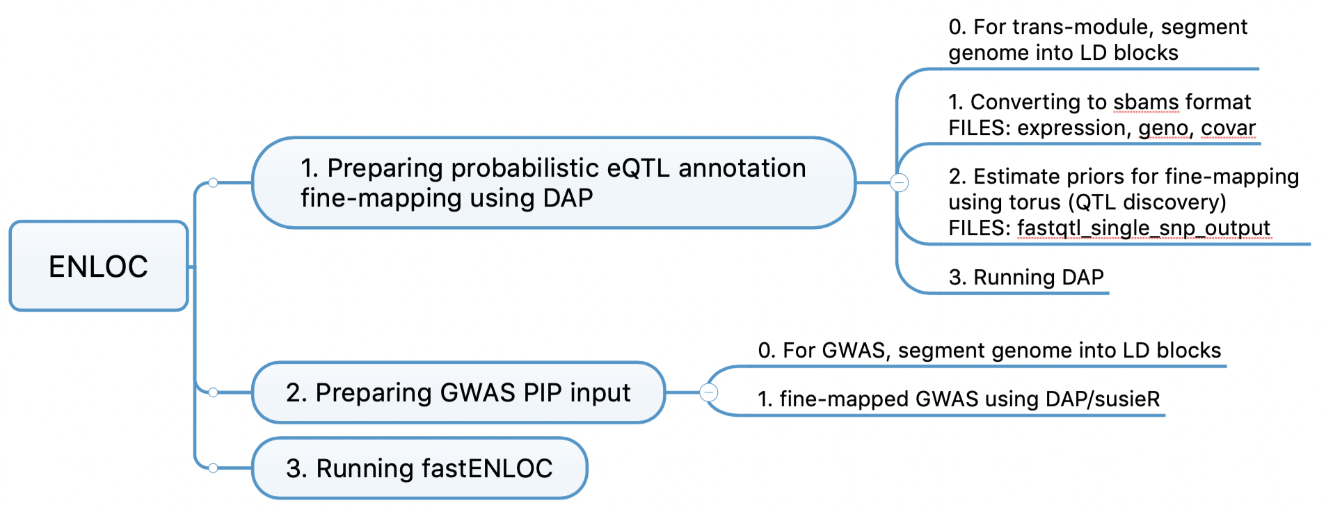
enloc code workflow

Past versions of 1101_enloc_code_pipeline.png

Version	Author	Date
b27c4e1	liliw-w	2021-11-15

• Need to provide “expression file” for the first fine-mapping. But we don’t have this file in the case of a module being the “expression trait”.

• DAP can be applied to each LD block independently. independent LD block provided a working recipe to segment the full genome based on the population-specific LD structures.

• Example of using enloc for colocalization: GTEx 2020. Used for “cis-QTL-GWAS colocalization: ENLOC.”

coloc

Paper-coloc single, Paper-coloc multiple:

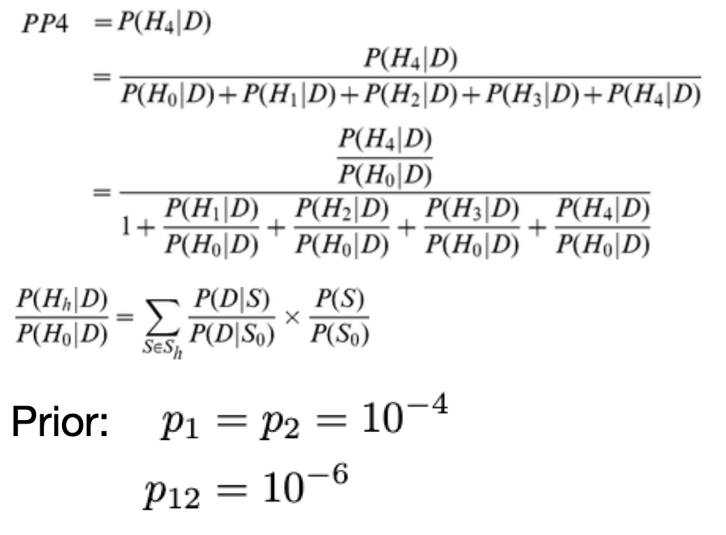
coloc equation

Past versions of 1101_coloc_theory.png

Version	Author	Date
b27c4e1	liliw-w	2021-11-15

Code tutorial:

First, segment the whole genome. Then fine-map each traits by susieR, better than coloc.abf as it allows multiple causal variants. Finally, coloc.

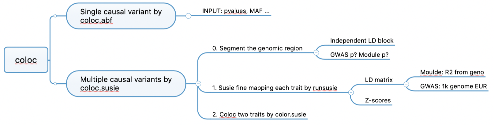
coloc code workflow

Past versions of 1101_coloc_code_workflow.png

Version	Author	Date
b27c4e1	liliw-w	2021-11-15

• Determine LD block? Independent LD block + small GWAS pvalue loci + small module pvalue loci

• Example of using coloc for colocalization:

  • Mu & Li: coloc + default prior.
  • GTEx 2020: Used for “Colocalization of cis- and trans-QTLs.”, coloc + default prior. In addition, used for “Colocalization of neutrophil ieQTLs and GWAS traits”: coloc + enloc prior.

Ref

Oct 25

Pan UKBB website

See website here.

Files website here.

• SNPs: 28,987,534 variants
• Trait:
• Population? meta? for (\(\beta, \text{se}, p, \text{low_confidence}\))

Trait

• category: A categorization of the phenotype

blood related traits:

1. “Biological samples > Assay results > Blood assays > Blood count”

e.g. Platelet count, Monocyte percentage, el al

2. “Biological samples > Assay results > Blood assays > Blood biochemistry”

e.g. HDL cholesterol, Rheumatoid factor, et al

3. “UK Biobank Assessment Centre > Physical measures > Blood pressure”

4. “Chapter III Diseases of the blood and blood-forming organs and certain disorders involving the immune mechanism …”

e.g. anaemias, D57 Sickle-cell disorders, el al

• pheno_sex: Use which one? “both_sexes”, “females”, “males”

• modifier: irnt or raw?

Variants filtering

summary statistics with low-confidence statistics removed and only considering high-quality variants.

• af: allele frequency
• low_confidence: criteria about allele count; includes some (non-exhaustive) basic quality control filters.
• high_quality: A boolean corresponding to a high-quality variant based on these filters … on “Files website”.

October 07, October 18

MSigDB gene modules, incorporated with DGN genes

MSigDB hallmark gene sets have 50 clusters, consisting of 4383 genes. 3276 genes are included in 12132 DGN genes (without removing cross-mappable genes).

Run Trans-PCO on the MSigDB hallmark gene sets.

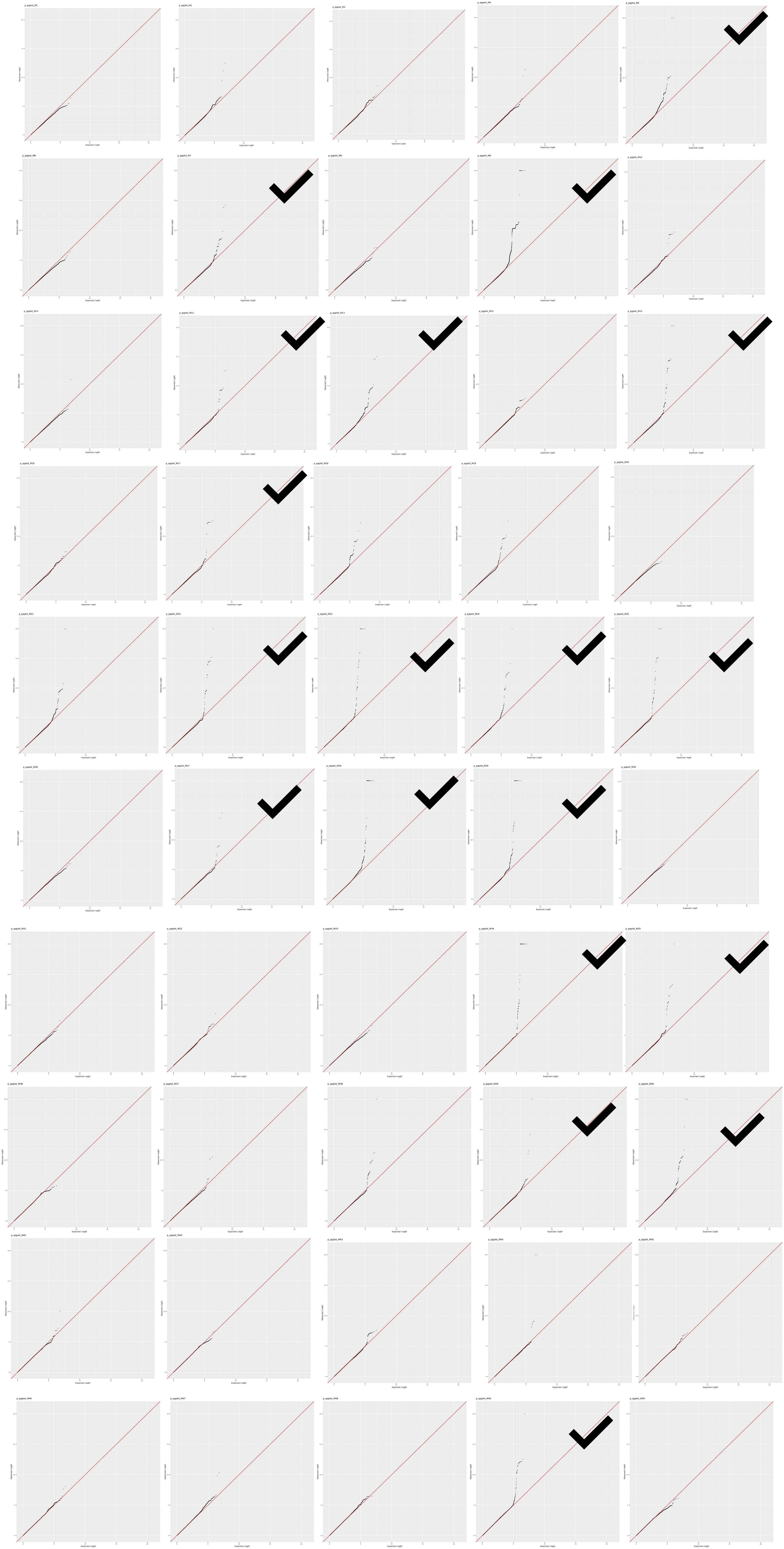
pvalues’ distribution - qqplot

Marked modules with significant signals by eye. See figure here.

Signals under empirical FDR

1. signals summary, under FDR 0.05, 0.1

FDR level	#signals	#unique signals	#independent signals
0.05	808	321	23
0.10	965	411	42

cross-mapped genes in 50 gene sets? already removed cross-mapped reads?

2. module (with annotation, size) v.s. chromosome signals

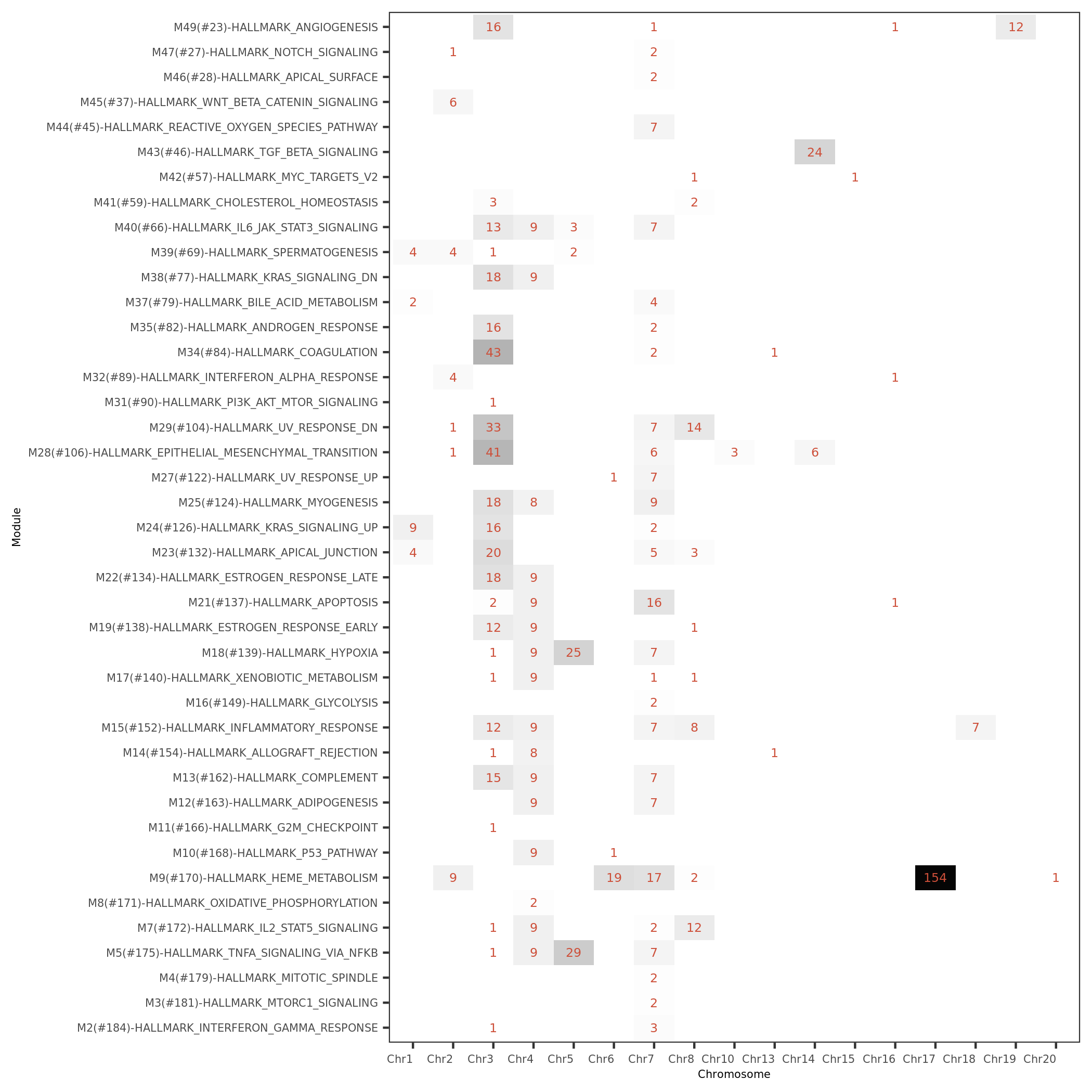
#signals of MSigDB modules for each module v.s. chr.

Past versions of 1018-num_signals_module_vs_chr_.png

Version	Author	Date
b27c4e1	liliw-w	2021-11-15

STRING PPI interaction network, clustered by hierarchical clustering.

Out of 12132 DGN genes, 11911 genes in the data included in STRING PPI network. As a result of hierarchical clustering, 11911 genes consist of 198 modules, with module size ranging from 210 ~ 26.

Run Trans-PCO on these modules.

pvalues’ distribution - qqplot

A selected set of modules.

Marked modules with significant signals by eye. See figure here.

DGN_no_filter_on_mappability

Without removing genes with mappability issues.

pvalues’ distribution - qqplot

October 04

Molecular Signatures Database

The MSigDB gene sets are divided into 9 major collections: the hallmark gene sets, and C1 - C8 gene sets.

Hallmark gene sets

What? Hallmark gene sets summarize and represent specific well-defined biological states or processes and display coherent expression.

How? These gene sets were generated by a computational methodology based on identifying gene set overlaps and retaining genes that display coordinate expression.

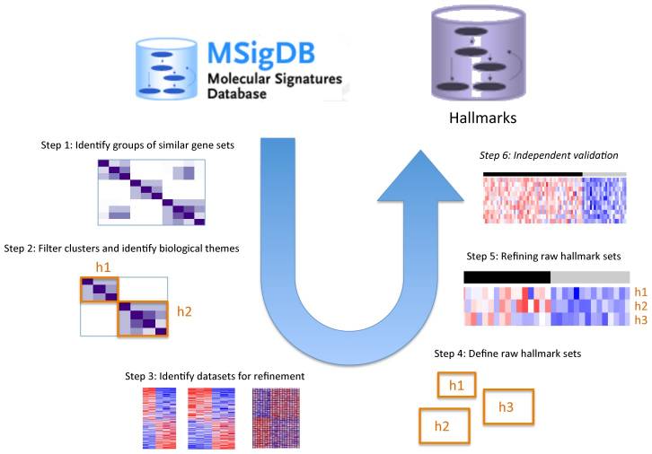
Pipeline to obtain hallmark gene sets from other MSigDB gene sets.

Past versions of 1004_hallmark_pipeline.jpeg

Version	Author	Date
b27c4e1	liliw-w	2021-11-15

See paper here.

pros? The hallmarks reduce noise and redundancy of the original overlapping gene sets, from which a hallmark is derived (‘founder’ sets).

Initial release. 50 hallmark gene sets. Comprise 4,022 original overlapping gene sets from 8,380 v4.0 MSigDB gene sets of collections C1 through C6.

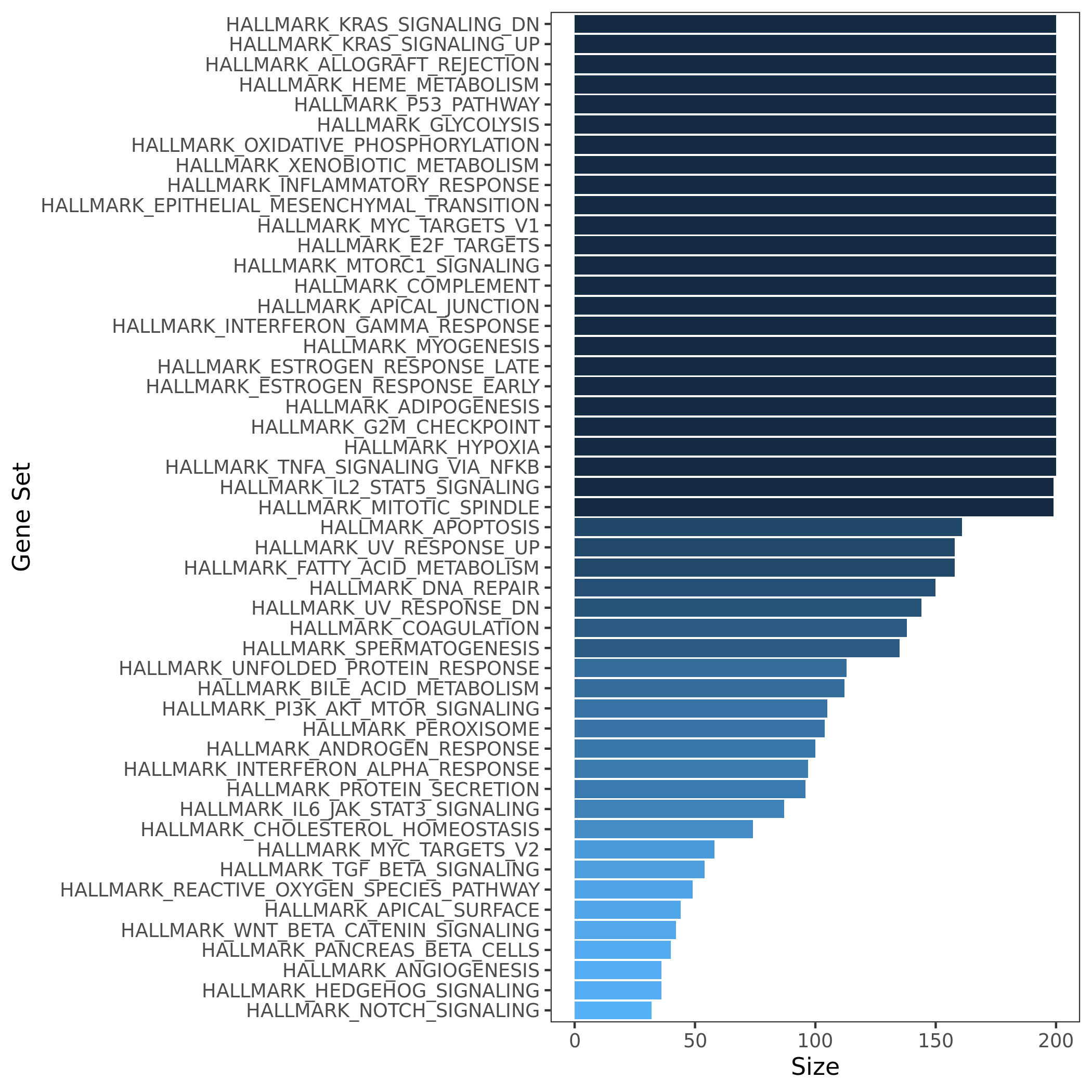
50 hallmark gene sets size

Past versions of 1004_geneSet_size_h.all.v7.4.symbols.gmt.png

Version	Author	Date
b27c4e1	liliw-w	2021-11-15

Summary of the hallmark gene sets: name, process category, description, number of founder sets and number of genes it contains. Table.

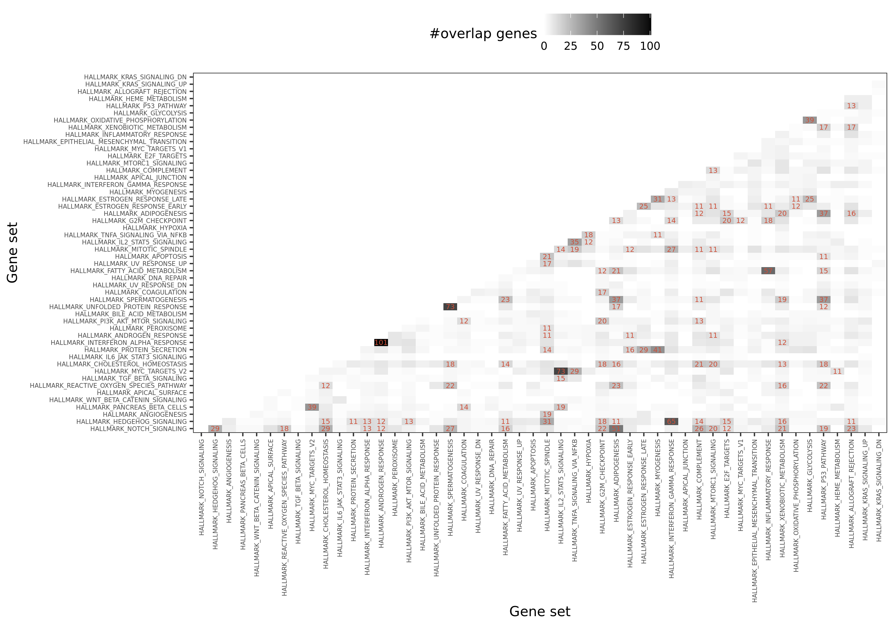
Overlapped genes among 50 hallmark gene sets

Past versions of 1004_geneSet_overlap_h.all.v7.4.symbols.gmt.png

Version	Author	Date
b27c4e1	liliw-w	2021-11-15

September 30

STRING PPI networks + Hierarchical clustering

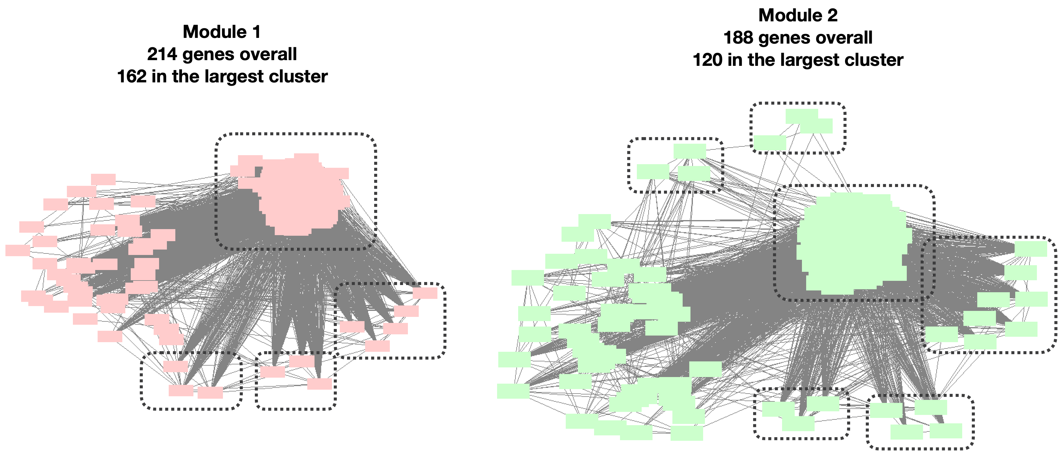
Question: Do the clusters make sense? Are the large clusters too loose or the small clusters too tight?

• Large clusters too loose such that can be separated to a few smaller cluster?

I looked at the top two largest clusters: Module 1 with 214 genes, and Module 2 with 188 genes.

Past versions of 0930_stringPPI_large_module.png

Version	Author	Date
b27c4e1	liliw-w	2021-11-15

• Small clusters too tight such that can be merged into less bigger cluster?

I looked at the last three smallest clusters: Module 194, 193, 192, with 23, 26, 26 genes, correspondingly.

Past versions of 0930_stringPPI_small_module.png

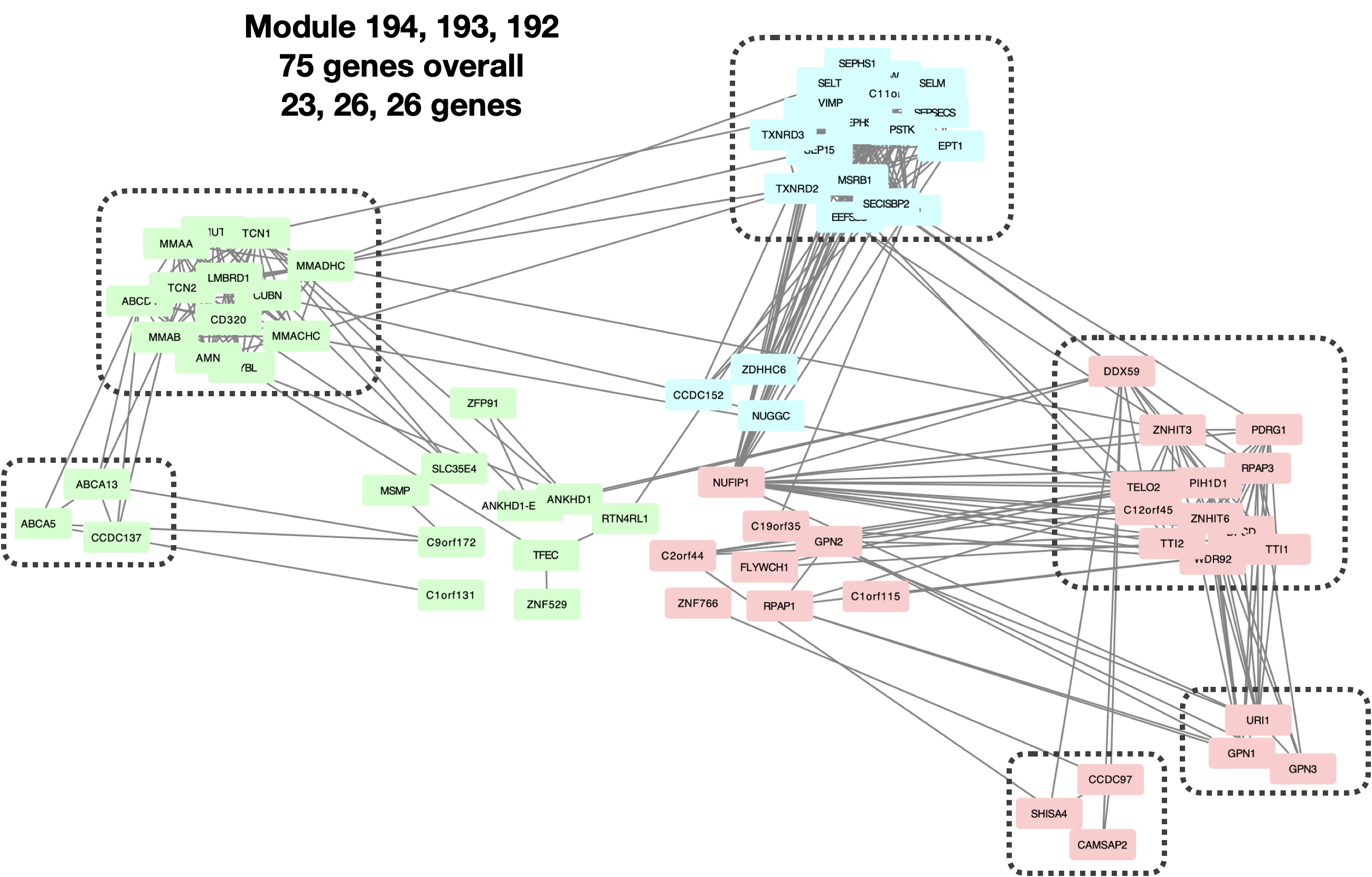
Version	Author	Date
b27c4e1	liliw-w	2021-11-15

Septermber 23

STRING PPI networks

Data

• Protein network data downloaded from here.

• Out of 12132 DGN genes, 11911 genes in the data included in STRING network, with 3076398 edges.

Clustering

A paper reviews a list of PPI networks clustering methods.

Clustering approaches to PPI networks can be broadly categorized as topology-free and graph-based ones. Topology-free approaches use traditional clustering techniques using notions of distance between proteins that do not take into account the topology of the network. Graph-based clustering approaches consider instead the topology of the network, and usually rely on specialized clustering techniques.

1. MCODE & MCL

   Too many genes for MCODE, I waited 1h and there was no result coming out.

2. Hierarchical clustering from clustermaker & R

   Hierarchical clustering in the Cytoscape plug-in, clustermaker, can’t handle so many genes. So I tried to do hierarchical clustering in R.

   Specifically, I used the “PPI scores” between two genes as the similary measurement for computing distances. Those gene pairs without edges (no PPI interaction) have 0 scores and 1 distance. Genes with itself have 1 scores and 0 distance (diagonals of distance matrix). Then I used the hclust in R to construct the hierarchical tree, and the dynamic tree cut cutreeDynamic for branch cutting, as used in WGCNA.

   As a result, 11911 genes consist of 198 modules, with module size ranging from 210 ~ 26.

HumanBase predicted tissue-specific interactions

Data

• Blood tissue interactions downloaded from here.

Clustering

1. functional module detection

2. MCODE (graph-based clustering, since only have edge info)

September 02, September 07, September 10

Pre-filter cross-map genes before grouping genes into modules

Out of 10461 genes, (after filtering based on meta info, protain and lincRNA, low mappability), do additional gene filtering if genes have too many cross-map genes (e.g. use 1K as the threshold). 4314 genes are removed.

As a result, 6147 genes are remained and are grouped in 95 modules.

Computation time

Problem

Last time, we ran into the problem that it is computational unfeasible if we want to run PCO without removing cross mappable genes in the previous step. See the illustration in the following figure.

There are two main steps that need long computational time. (1) For each SNP, remove genes from the module that are cross mappable with cis- genes of the SNP. (2) In this case, we would have module containing different genes for SNPs with different cis- genes, thus different \(\Sigma\) and \(\Sigma^O\). Therefore, tremendously increase the computational time.

Try solution 1: filtering SNPs instead

One of the possible solutions we mentioned is, instead of filtering genes for each SNP, we can try filtering SNPs and keeping the module unchanged. That being said, if a SNP has cis- genes cross mappable with any genes in the module, then this SNP is removed from the following PCO analysis.

In this way, there are two advantages. First, it’s faster to filter SNPs than genes. Second, we will have same module for all remained SNPs, thus same \(\Sigma\) and \(\Sigma^O\).

So, next I check how many SNPs will be left after this filtering step.

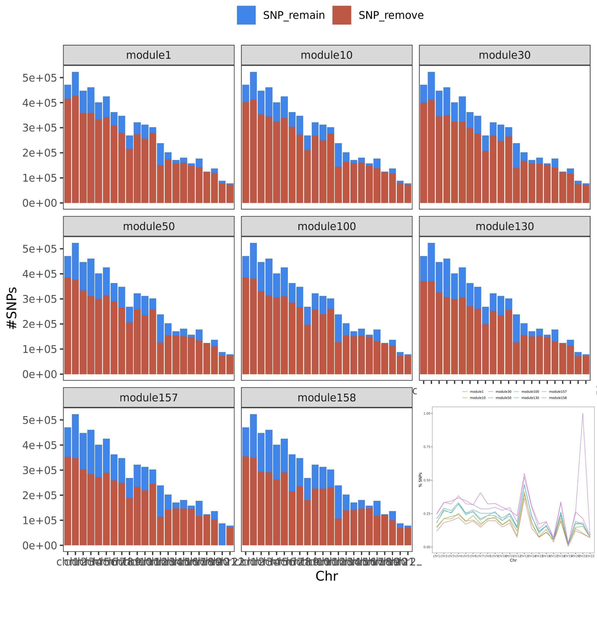
Figure. SNP remained. The bar plot gives the number of SNPs, while the line plot gives the percentage of the remained SNPs on each chr.

Past versions of 0907_SNP_remain.png

Version	Author	Date
b776926	liliw-w	2021-09-07

We can see, if we filter SNPs instead, over half of the genome will be removed from the p-value analysis. We could miss a lot of signals.

Keep cross mappable genes in the filtering step

1. Genes and modules containing cross mappable genes

All genes:	13634
With meta:	12585
Final use:	10461
All removed:	3173
including:	meta: 1049 auto: 1 prote&linc: 453 low_map: 1798 cross_map: 0
Number of modules:	158

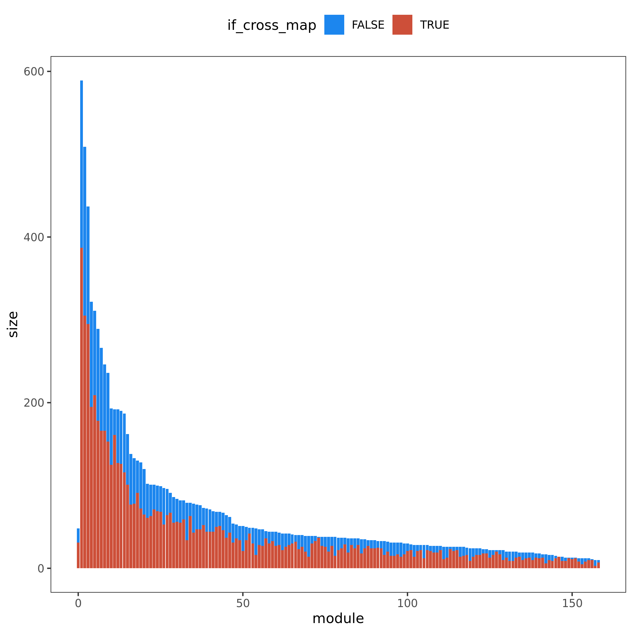
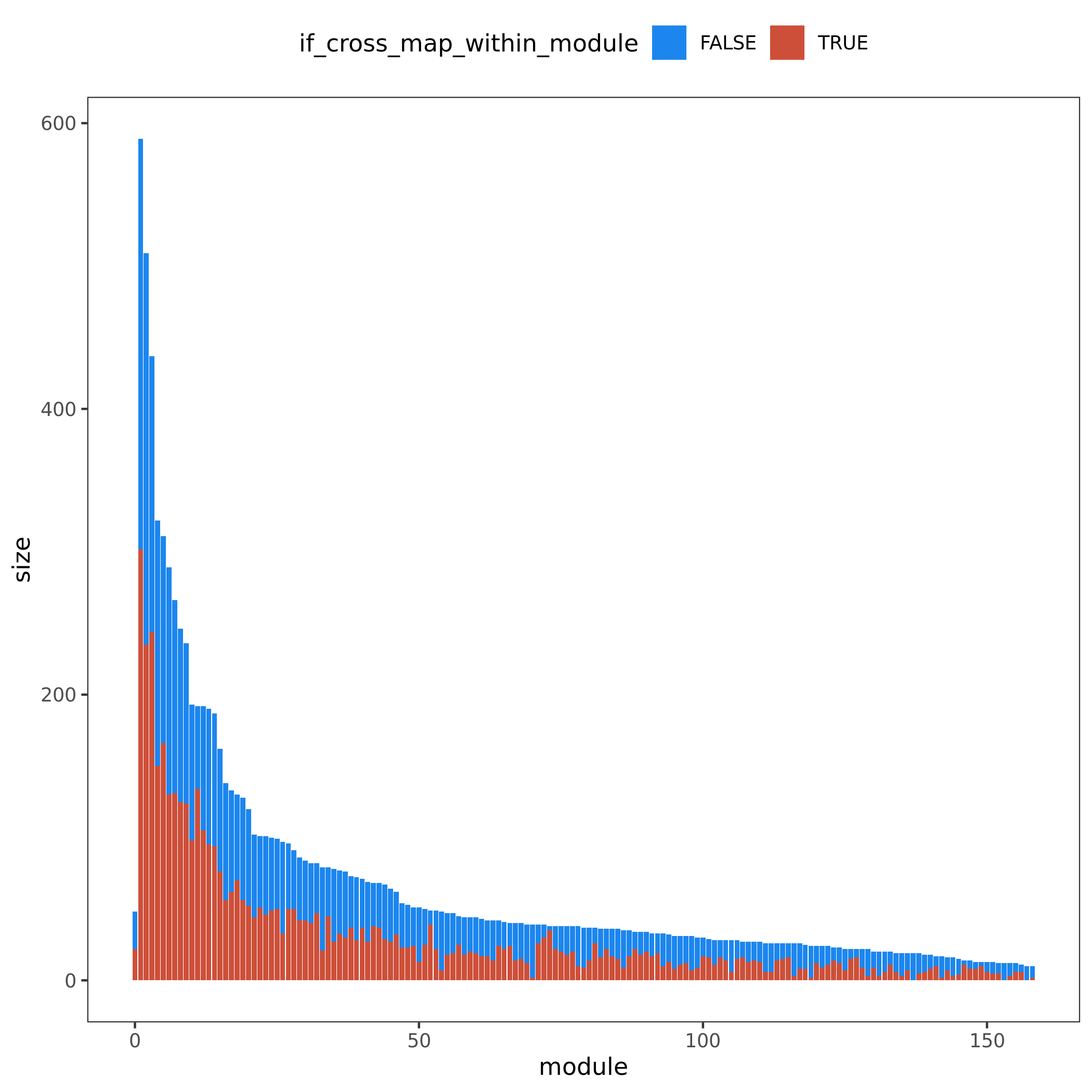
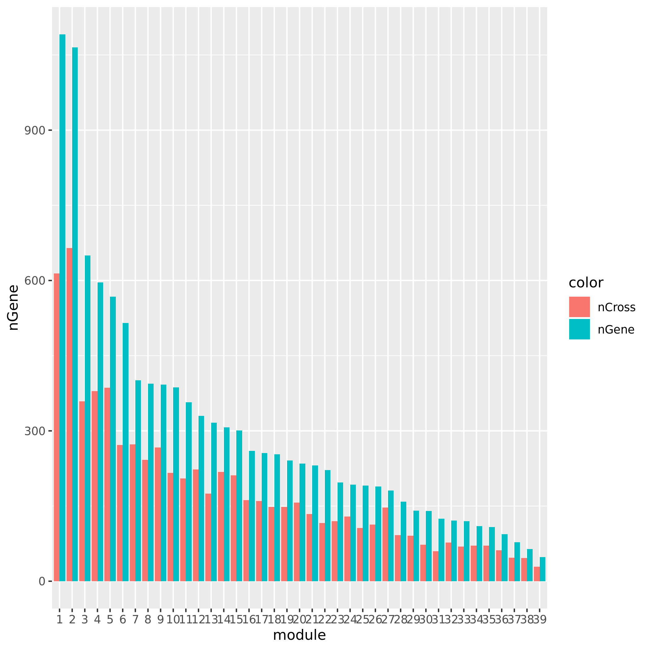
Figure. Module v.s. #Genes. Bar height for module size. Red/blue bar for #cross mappable genes for each module. Left for genes cross mappable with any genes. Right for genes cross mappable with genes within the same module.

2. Run PCO with cross mappable genes

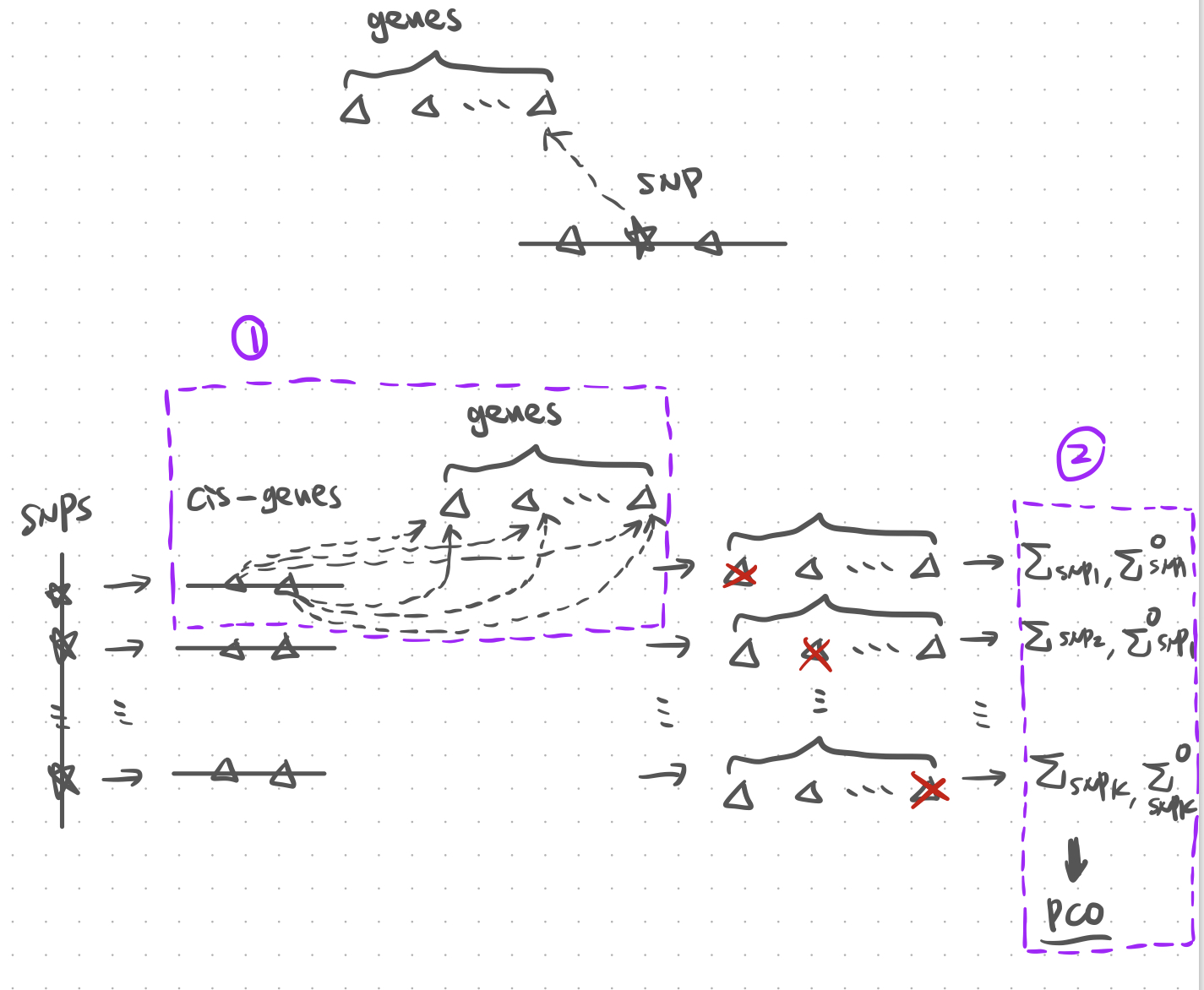
Figure. Illustration of PCO with cross mappable genes.

Past versions of 0902_PCO_keep_crossmap.jpeg

Version	Author	Date
786b185	liliw-w	2021-09-02

Problem: Computational infeasible

• In phase 1, for each SNP, filter out genes within the module that are cross mappable with any of its cis- genes. Not fast, as need to search pairs of (cis- gene, module gene) in the cross-mappability file with 23,727,385 cross-mappable gene pairs.

The code I use,

if_cross <- sapply(cis_Genes[1:10], function(x){
  colSums(matrix(outer(x, module_Geneid, FUN = "paste", sep=";") %in% cross_map$V4 |
                   t(outer(module_Geneid, x, FUN = "paste", sep=";")) %in% cross_map$V4, ncol = length(module_Geneid)) ) == 0
} )

Time elapsed,

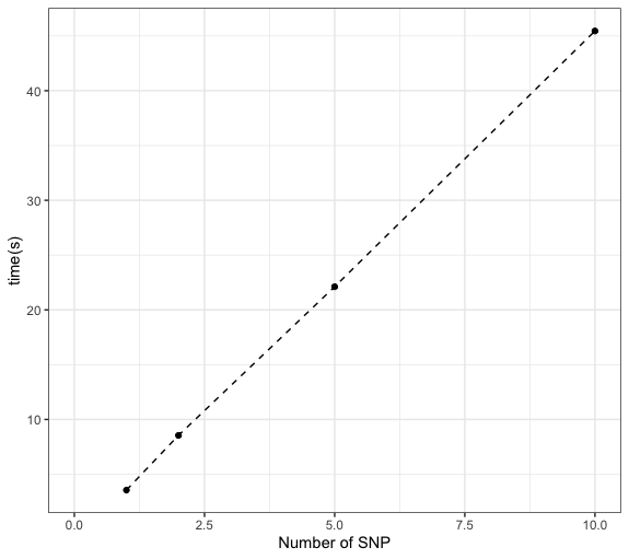
Figure. Time used for a SNP with ~40 cis- genes and a module with 15 genes.

Past versions of 0902_time_cross_map.png

Version	Author	Date
786b185	liliw-w	2021-09-02

• In phase 2, each SNP could correspond to modules with different gene combinations, thus diff. \(\Sigma\) for with-in module correlation and \(\Sigma^0\), which is the estimated correlation of six tests involved in PCO using 2000 simulations. Thus, computing \(\Sigma^0\) for each SNP should take a long time.

July 08

How expression PCs affect the signals?

The following table gives the number of unique signals under various FDR levels for DGN regressing out expression PC as covariates (“DGN_wo_expPC”) and keeping expression PCs (“DGN_with_expPC”).

FDR level	DGN_wo_expPC	DGN_wo_expPC_maxp	DGN_with_expPC	DGN_with_expPC_maxp	overlap	#*
0.05	313	1.9e-08	169	4e-09	125	218
0.10	512	6.5e-08	225	2e-08	167	303

Correlation between meta-ed gene zscores from eQTLGen

Check document here.

July 06

How Sigma \(\hat{\Sigma}_{DGN_exp}\) and \(\hat{\Sigma}_{nullz}\) affect PCO pvalues for DGN?

I inspected three modules. Check here for the comparison.

For individual and clearer figures, check here, here, here, here, here, here, here, here, here.

June 29

“Try using zscores to build sigma, plot of number of SNPs with low zscores”

1. plot of number of SNPs with low zscores

In this section, I am going to check how the estimated Sigma \(\hat{\Sigma}_{K}\) (correlation matrix of zscores/residule expression across genes) can affect PCO’s pvalues. Use eQTLGen zscores. Consider two \(\hat{\Sigma}\)’s. (1) \(\hat{\Sigma}_{DGN}\), computed by \(cor(\tilde{Y}_{n \times K}^{DGN})\), where \(\tilde{Y}\) is the residual expression data from DGN, n is sample size, K is gene module size. (2) \(\hat{\Sigma}_{nullz}\), computed by \(cor(\tilde{Z}_{m \times K}^{eQTLGen})\), where z is genome-wide independent null zscores from eQTLGen, m is the number of null SNPs (m is in fact much less than genome-wide, but should be sufficient?).

Since for each null SNP, we should have its zscores on all genes (or at least all genes in the module we consider), but eQTLGen doesn’t provide zscores for all genome-wide SNPs (only disease-related variants for trans-eQTLs and close-to-gene variants for cis-eQTLs). Therefore, I will first extract the common SNPs for each module. Main steps include:

• Combine the zscores of all the significant/non-significant gene-SNP pairs in both eQTLGen cis-eQTL and trans-eQTL results.

• For each module, extract the common SNPs that have zscores available for all genes in the module.

• For each module, further extract the common SNPs that are “NULL SNPs”. A snp for a module is defined as a “null snp” if its z-scores for all genes in this module are below some z-score cutoff (i.e. all z-scores are small z’s").

• Among these common null SNPs, check how many of them are independent. (Use DGN genotype ‘plink –indep-pairwise 50 5 0.2’ ??? in this case, some SNPs not included in DGN are also considered as "independent. ref panel including all eQTLGen snps?)

Past versions of 0629_num_nullSNP.png

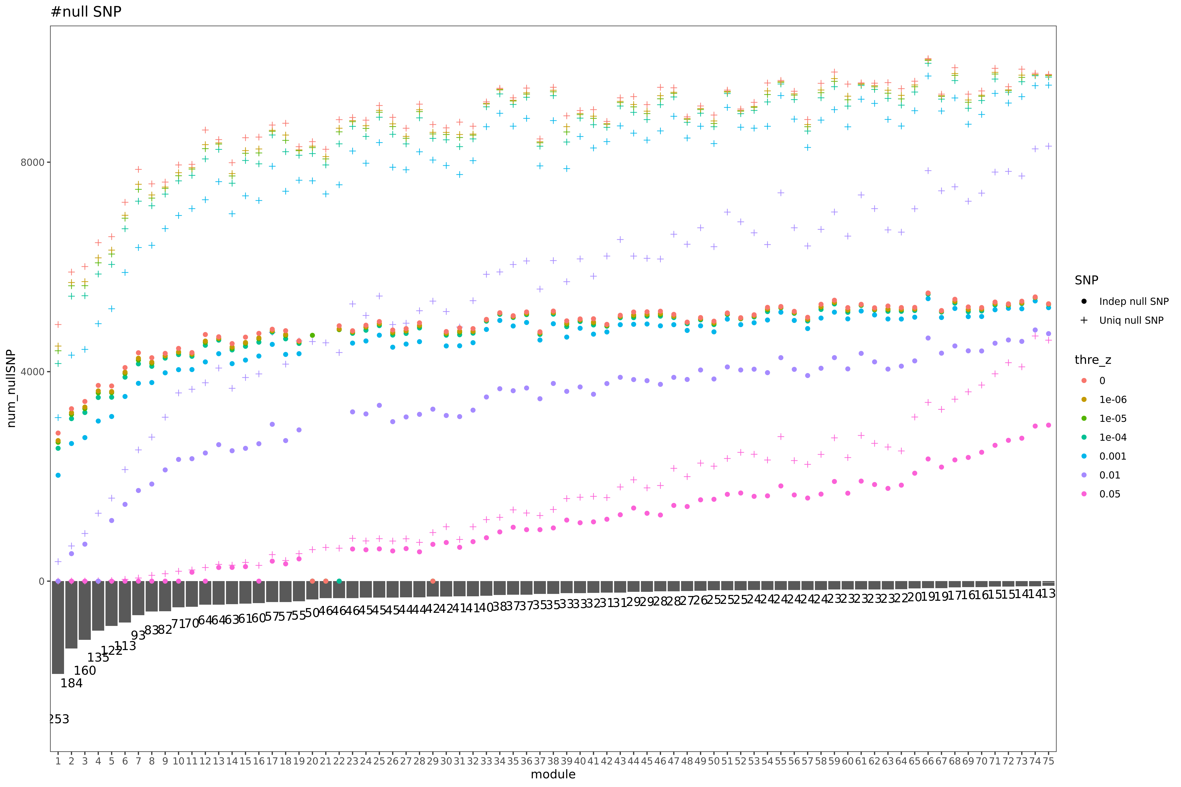
Version	Author	Date
1b79abb	liliw-w	2021-06-29

Here I explain the above figure. x-axis is for each module (75), y-axis is for number of SNPs under various scenarios that can be used for computing \(\hat{\Sigma}_{nullz}\). Color is for various z-scores cutoff for defining “NULL SNPs”. The cutoff is pvalue of z. Smaller cutoff, more insignificant z. Point shape is for unique SNPs and independent SNPs. The barplot in the lower panel gives the number of genes in each module.

Observations

1. For larger gene module, the common null SNPs (unique and independent) are fewer.

2. The average number of the unique null SNPs is ~8000 (under pvalue of z > 0.001). The independent null SNPs is ~4000.

3. Since we were particularly interested at eQTLGen’s module1, (as all eQTLGen trans-variants are significant for module1,) next I will focus on module1. I use the 2282 independent null SNPs (under pvalue of z > 0.001) for module1 to calculate \(\hat{\Sigma}_{nullz}(module1)\).

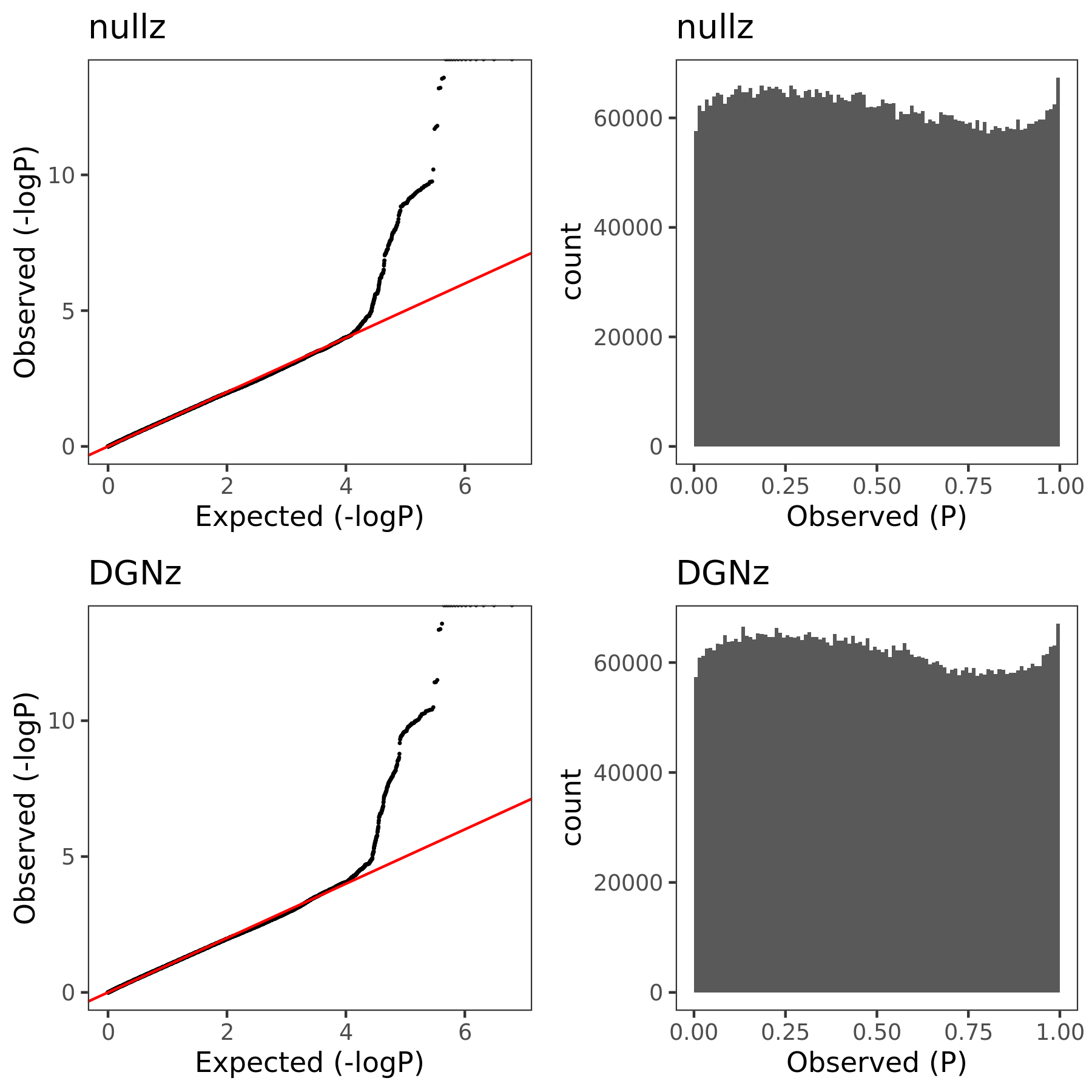
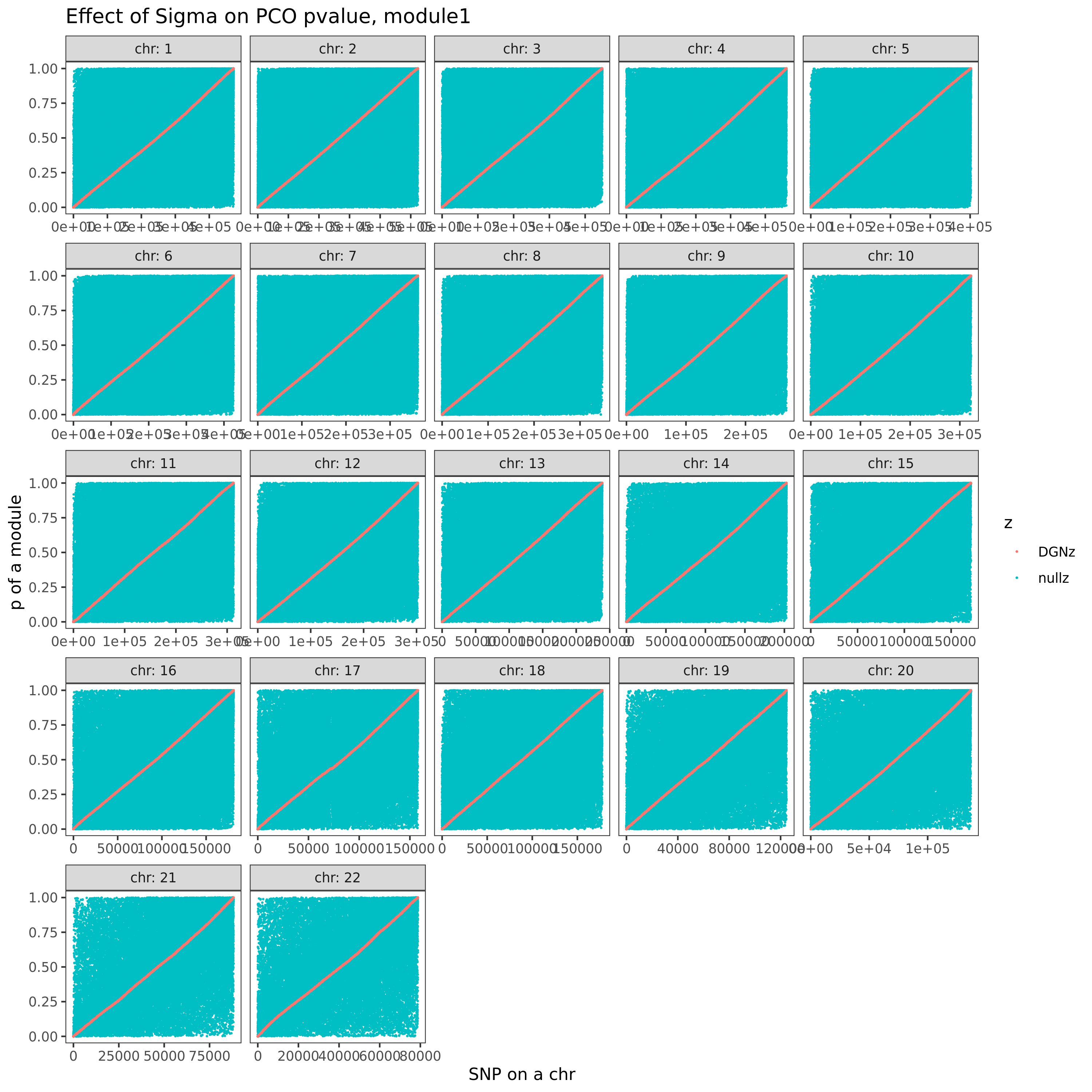
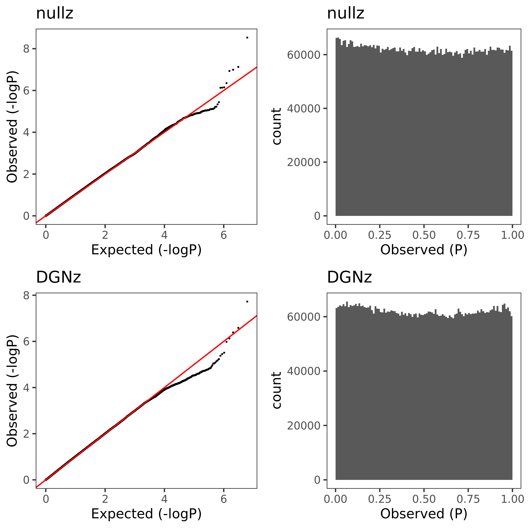
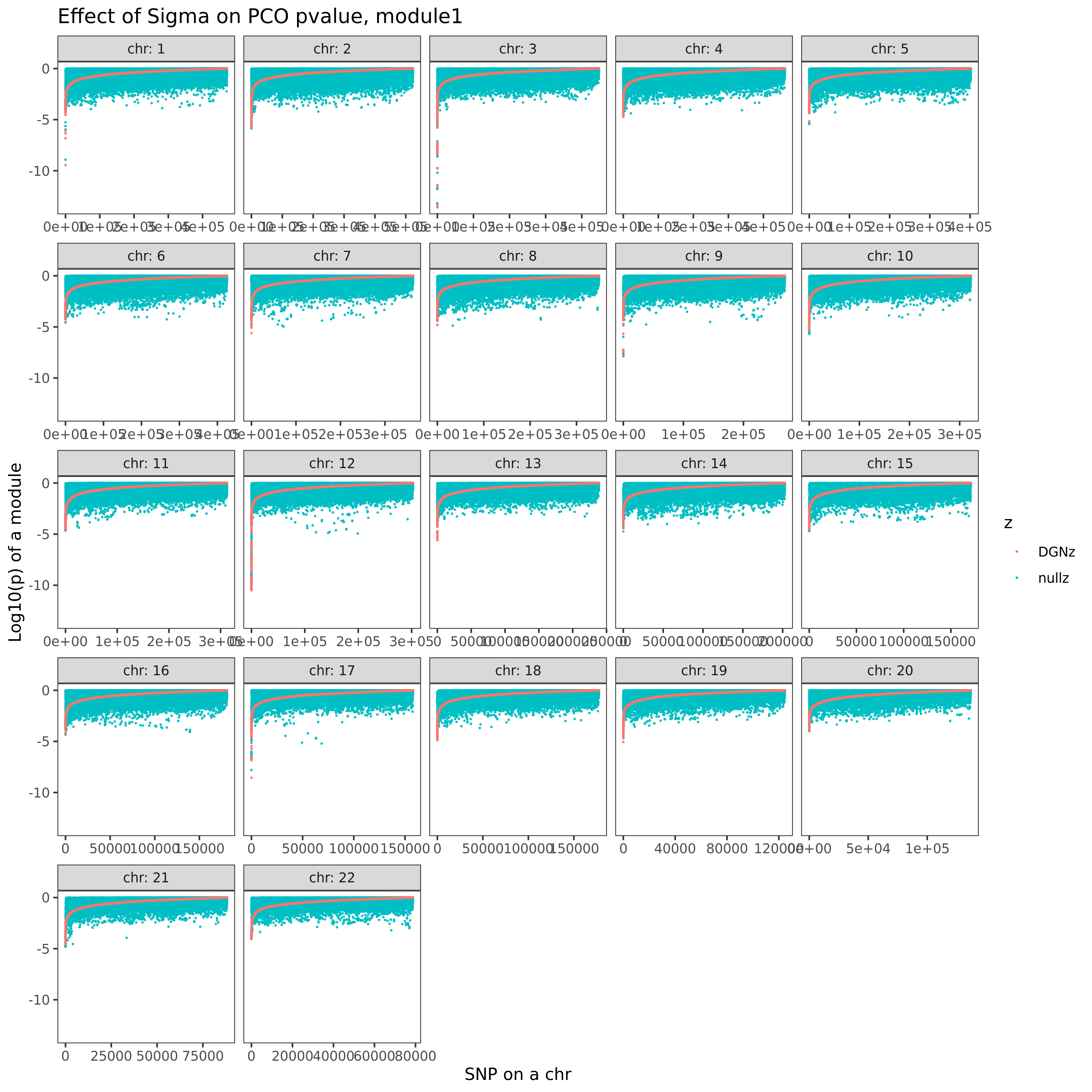
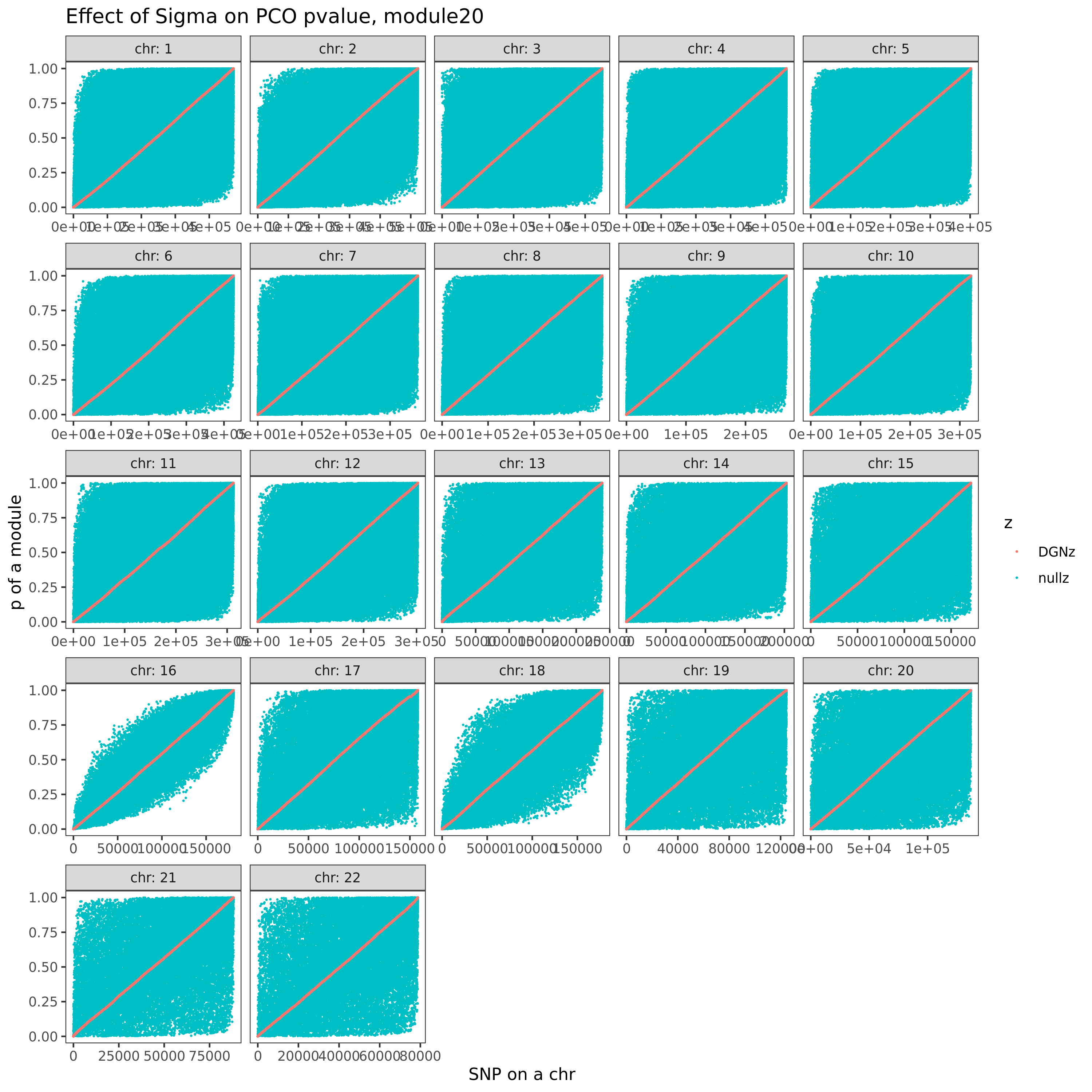
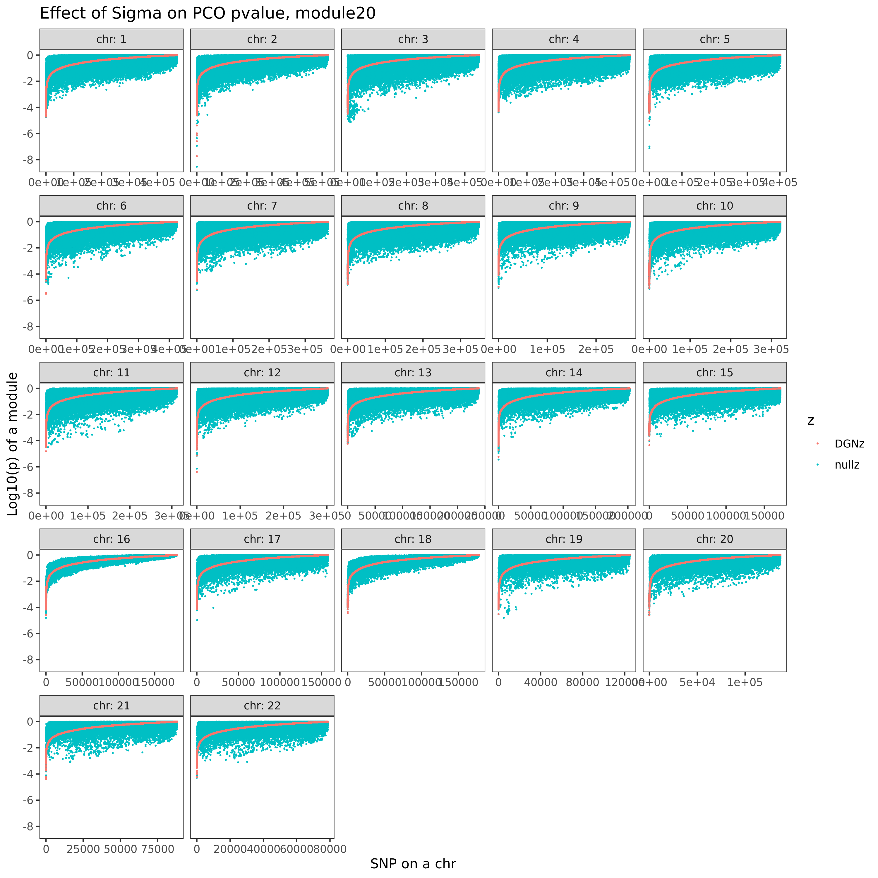
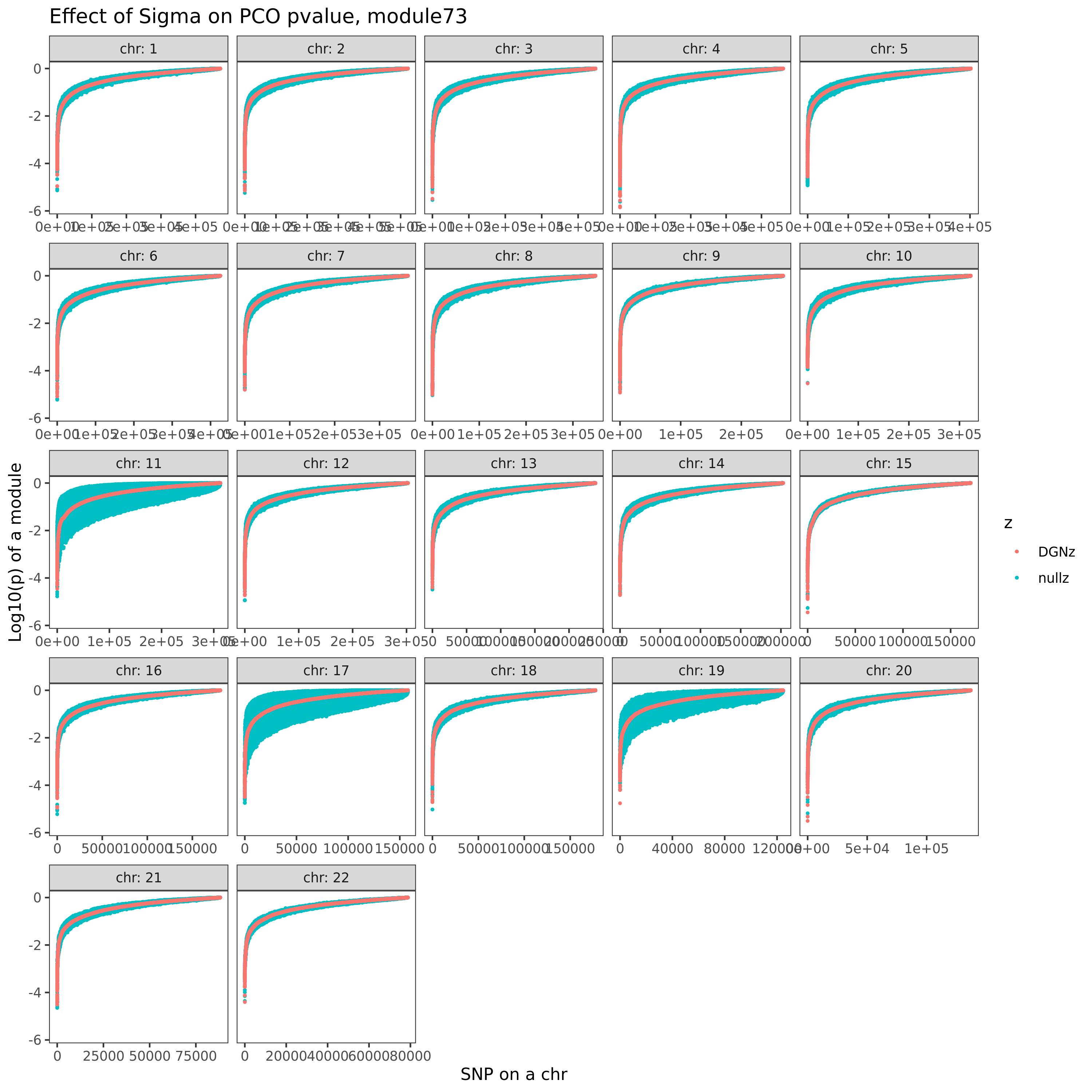
Build Sigma \(\hat{\Sigma}_{DGN}\) and \(\hat{\Sigma}_{nullz}\) and check PCO pvalues.

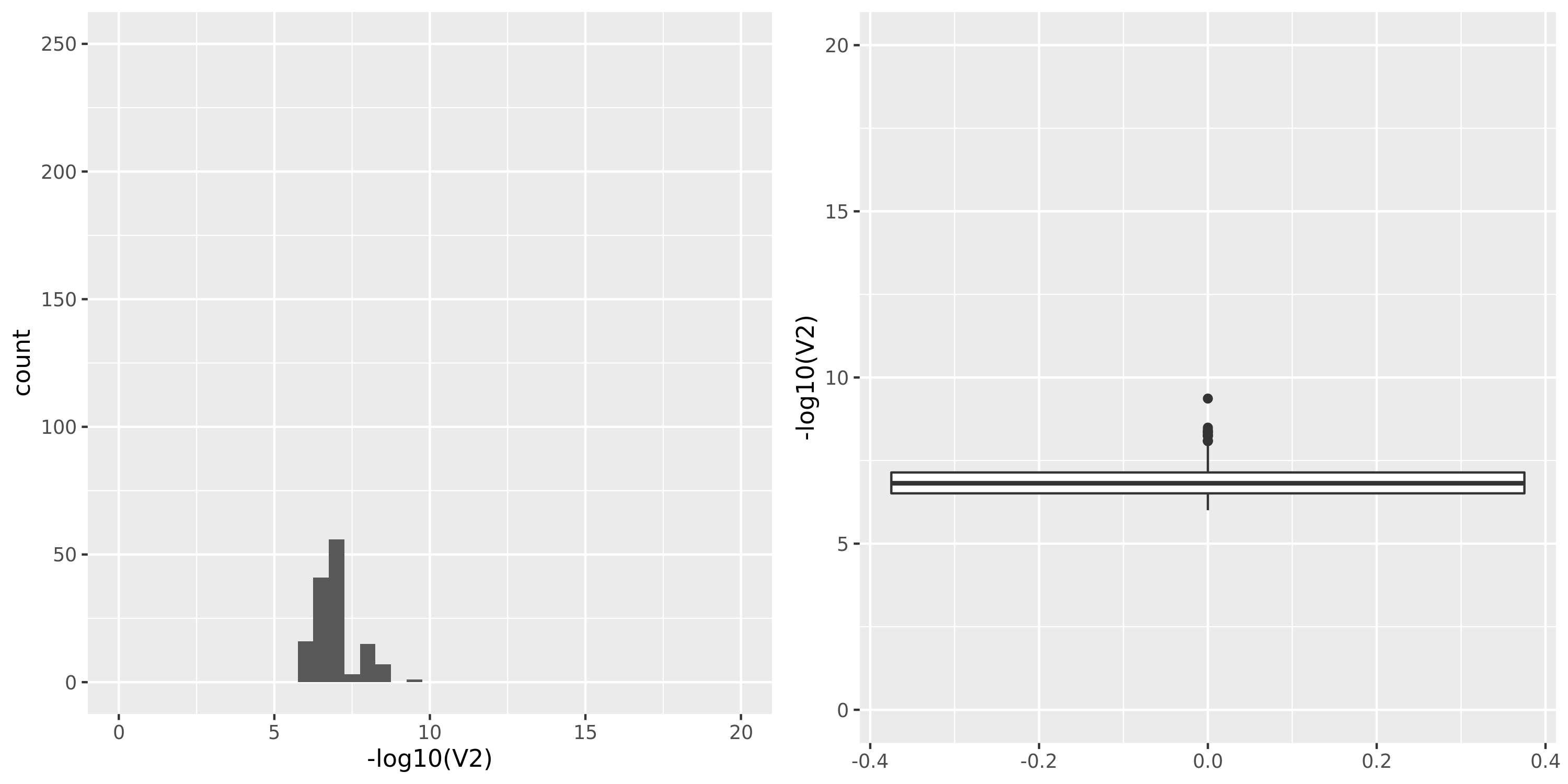
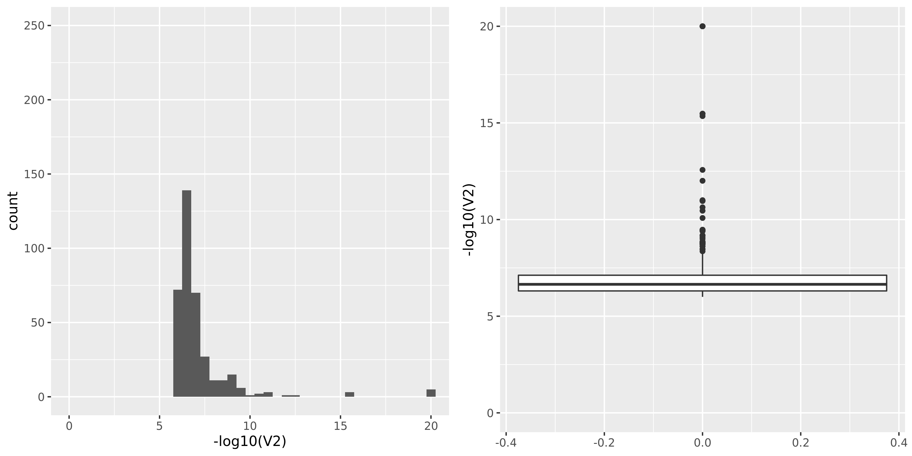
eQTLGen’s module1. Run PCO based on two Sigmas, \(\hat{\Sigma}_{DGN}\) and \(\hat{\Sigma}_{nullz}\) built on 2282 independent null SNPs. Calculate pvalues of 9918 SNPs across chromosomes.

Past versions of 0629_effect.of.Sigma.on.PCO.pvalue.module1.png

Version	Author	Date
1b79abb	liliw-w	2021-06-29

In the above figure, x-axis is for snp across chromosomes, y-axis is for log(p) for the module1, color is for different \(\hat{\Sigma}\), grey dashed line is the Bonferroni pvalue threshold (~1e-8).

Past versions of 0629_qqplot.effect.of.Sigma.on.PCO.pvalue.module1.png

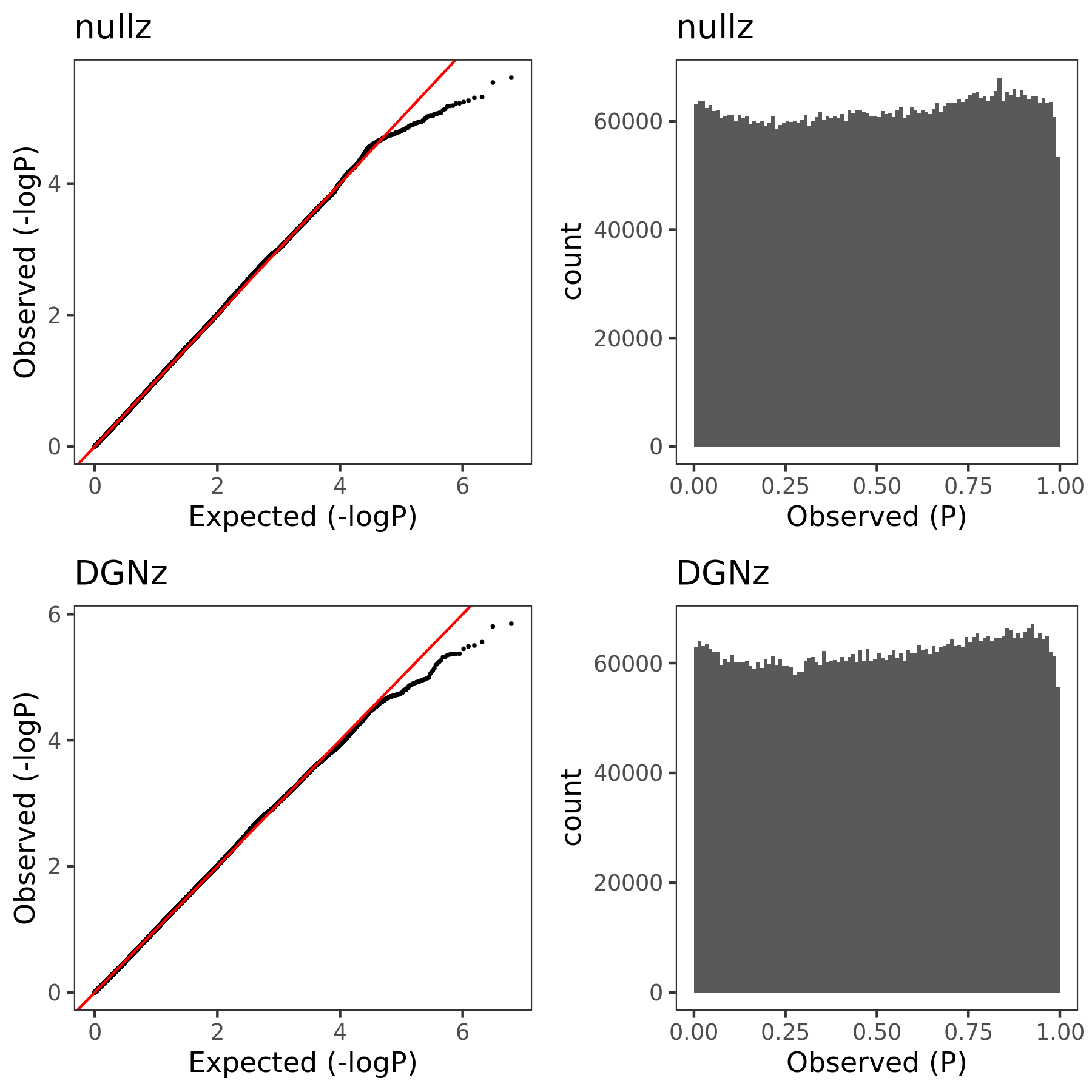
Version	Author	Date
1b79abb	liliw-w	2021-06-29

The above figure gives QQ-plot for all pvalues across 22 chr’s of module1.

Observations

1. Using \(\hat{\Sigma}_{nullz}\) gives larger PCO pvalues, than using \(\hat{\Sigma}_{DGN}\). Number of signals decreases. Under Bonferroni pvalue threshold (~1e-8), when using \(\hat{\Sigma}_{nullz}\), there are 790 out of 9918 SNPs are significant, compared to 9794 significant SNPs using \(\hat{\Sigma}_{DGN}\).

June 25

Replication of eQTLGen results in trans-PCO of eQTLGen summary stats?

I first give some data statistics here.

Dataset	Method	#(gene, SNP)/(module, SNP)	#unique genes/modules	unique SNPs
eQTGen	FDR<0.05	59786	6298	3853
eQTGen	filter	20394	1857	2469
eQTLGen_trans-PCO	qvalue	406729	75	9918
eQTLGen_trans-PCO	Bonferroni	55634	74	9915

• The eQTGen’s original result here gives 59786 (gene, trans-eQTL) pairs under FDR \(<0.05\), corresponding to 6298 unique genes and 3853 unique SNPs.

• After some filtering, to make sure the eQTGen trans-eQTLs and genes are included in out trans-PCO result using eQTLGen summary stats. There are 20394 (gene, trans-eQTL) pairs left, corresponding to 1857 unique genes and 2469 unique SNPs.

• Orignal eQTLGen_trans-PCO result (under qvalue FDR correction): 406729 (module, trans-eQTL) pairs, corresponding to all 75 unique modules and 9918 unique SNPs.

• Under Bonferroni correction (p<6.721785e-08): 55634, 74, 9915.

Next, I will check how eQTGen signals are replicated in eQTLGen_trans-PCO results (see bold text above). The basic idea is, for an eQTGen trans-eQTL, find its trans-target genes, then look at how these genes are distributed in each gene modules we used for eQTLGen_trans-PCO, and whether the corresponding (module, trans-eQTL) are identified by eQTLGen_trans-PCO. Specifically, I will check two things.

1. For a trans-eQTL whose trans-target genes are included in one of our PCO module, is this (module, trans-eQTL) identified by eQTLGen_trans-PCO? (Power)

   Since in previous analysis, the intuition is PCO tends to pick modules where there are multiple trans-target genes for a SNP. Therefore, in the below figure, I picked out all the eQTGen trans-eQTLs that have >2 target genes and plotted them on x-axis. The target genes are distributed on the Y-axis for each PCO module. Number/color is for #target genes. These (module, SNP) pairs should be significant in eQTLGen_trans-PCO. I circled out (red) those (module, SNP) pairs that are missed by eQTLGen_trans-PCO. As a result, 11 (module, SNP) (11 unique SNPs) are missed.

Power

Past versions of 0625_power.png

Version	Author	Date
9275134	liliw-w	2021-07-08

Check here for clearer version.

2. For a trans-eQTL whose trans-target genes are not included in any PCO modules (or only 1 or 2), is this (module, trans-eQTL) identified by eQTLGen_trans-PCO? (TIE)

   Similar plot, except Number/color is SNP with 0, 1, or 2 target genes in each module. These (module, SNP) pairs are less likely to be identified by eQTLGen_trans-PCO. Yet, I circled out (green) those (module, SNP) pairs that are still identified by eQTLGen_trans-PCO.

TIE

Past versions of 0625_TIE.png

Version	Author	Date
9275134	liliw-w	2021-07-08

Check here for clearer version.

Observation

1. Almost all eQTGen trans-eQTLs with >2 target genes and their corresponding module are identified by eQTLGen_trans-PCO. This may suggest a good power of eQTLGen_trans-PCO.

2. However, the false positiva rate may be inflated, as a large amount of SNPs that has no target genes in the modules are also identified. (Maybe although none of the genes in the module are target genes for the SNPs, the genes may be cross-mappable with the SNP’s other traget genes that are filter out?)

How does zero values affect qvalue?

Short answer:

June 14

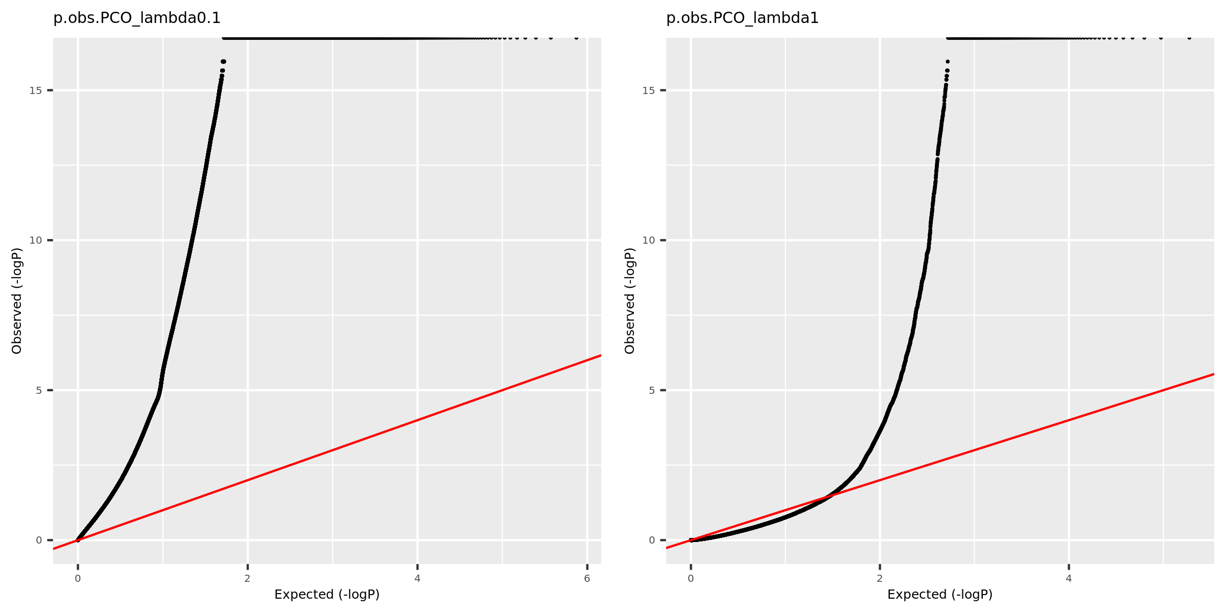
Why there are so many eQTLGen signals using PCO_\({\lambda<0.1}\)?

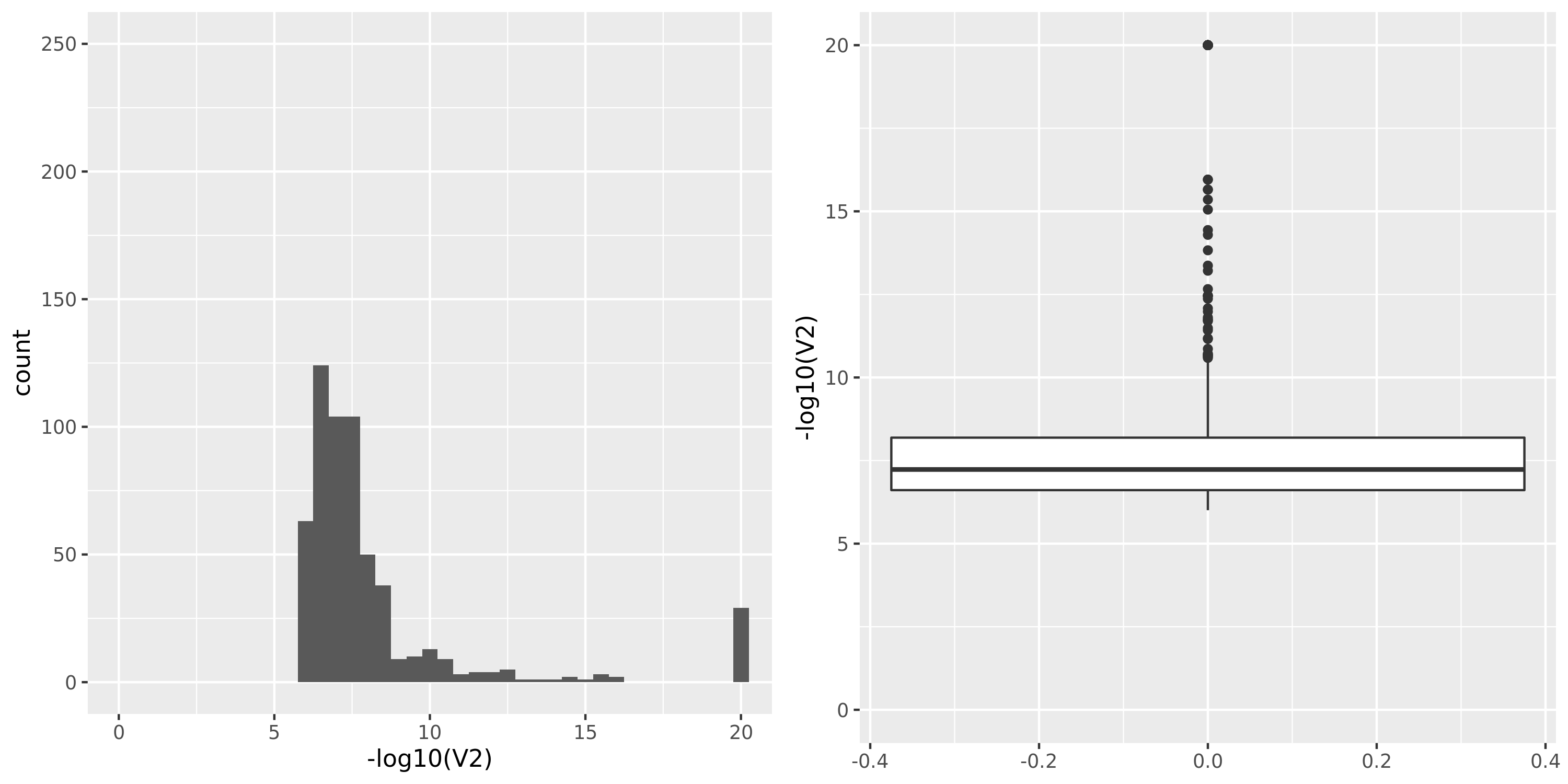
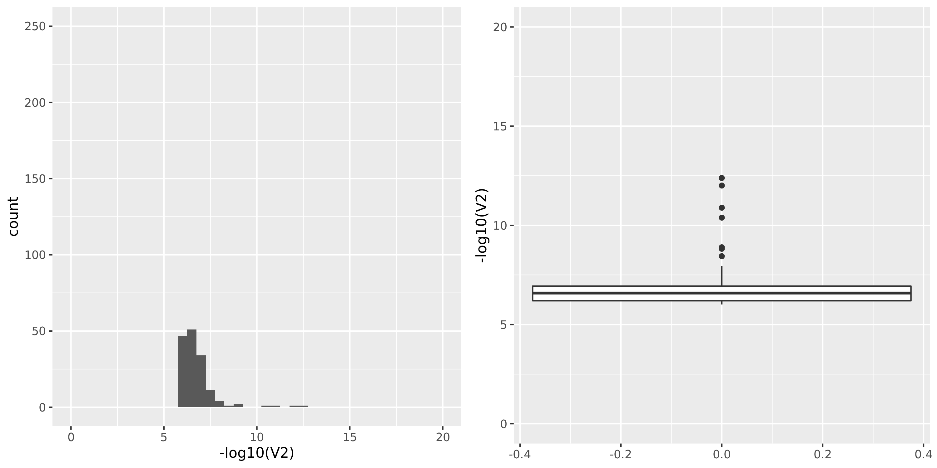
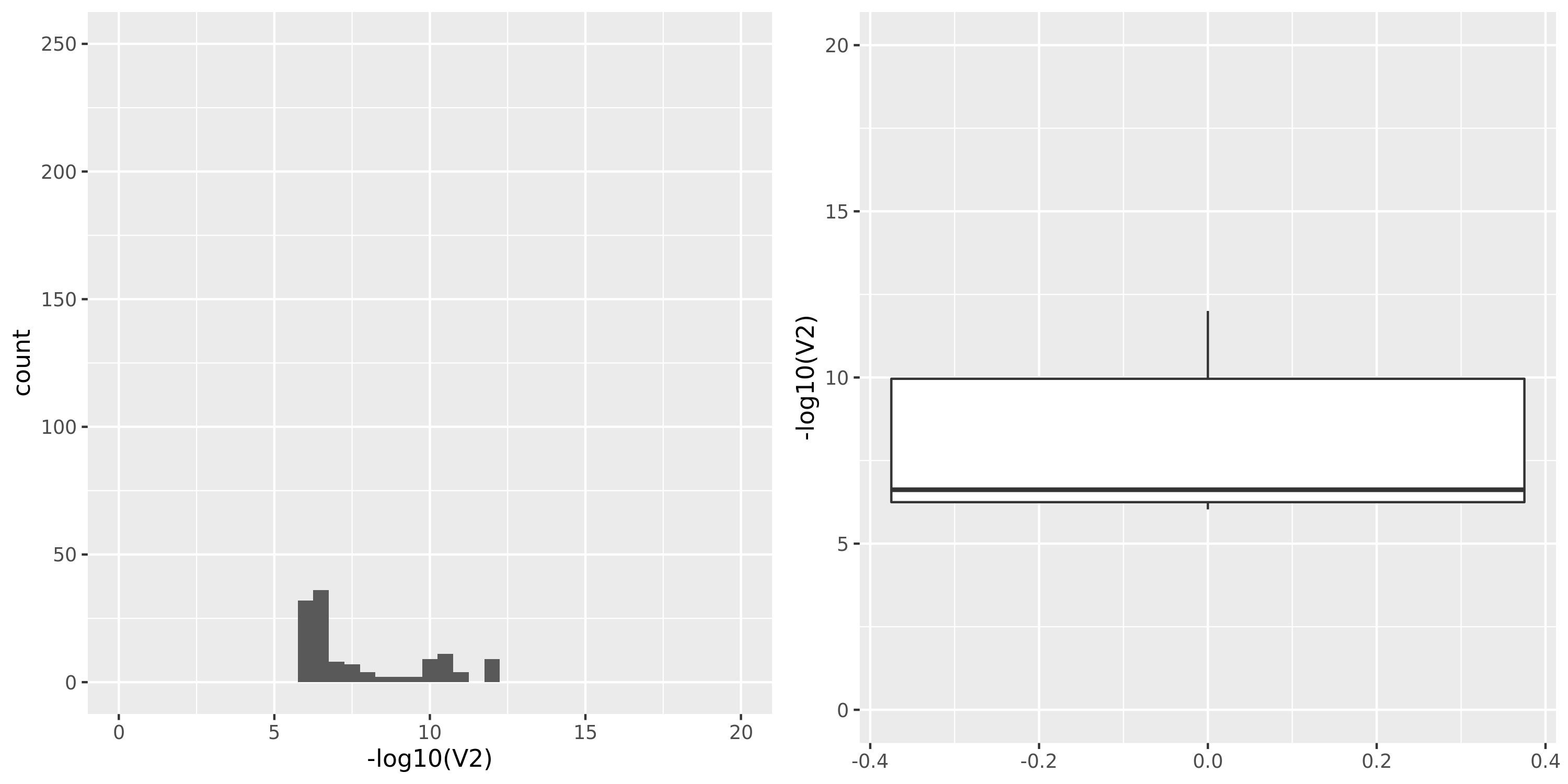
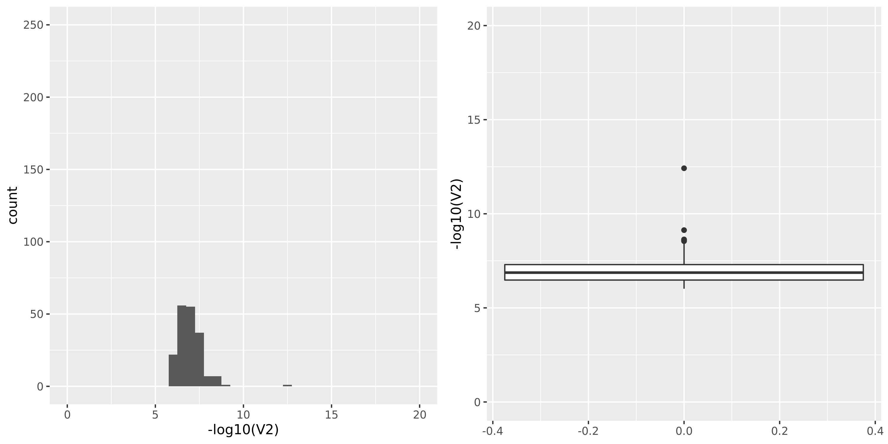
Check the QQ-plot of the observed pvalues from eQTLGen using PCO_\({\lambda<0.1}\) (9918 unique SNPs, all eQTLGen variants) and PCO_\({\lambda<1}\) (909 unique SNPs).

Past versions of 0614_qqplot.p_obs.eQTLGen.png

Version	Author	Date
9275134	liliw-w	2021-07-08

June 11

Compare with truncated ‘DGN_transeQTL_battle2014’

In this section, I removed trans-eGenes from Battle’s result that are not included in our analysis for being cross-mappable or poorly mapped. I do this to makes sure univariate and multivariate are based on the same set of genes. I go through the same analysis as below.

• Summary of the new version Battle trans-eQTL signals

After filter our some trans-eGenes, there are 157 (v.s. 736) significant (gene, SNP) pairs left, corresponding to 84 unique trans-eQTLs and 47 unique trans-eGenes.

The following is a a table of the number of trans-target genes of these 84 unique trans-eQTLs.

 1  2  3  4  5 15 16 29 
75  1  1  3  1  1  1  1 

We have identified 313 unique trans-eQTLs, among which 24 are also detected by Battle’s univariate method. The above table gives which Battle’s signals are replicated by trans-PCO.

Among 84 Battle’s trans-eQTLs, 24 (~28.57%) are also detected by trans-PCO. For 9 signals with more than one trans-target genes included in our analysis, all of them are detected by trans-PCO. Trans-PCO also detected other 15 signals with only one trans-target gene used in our analysis. For the other 60 univariate signals that are missed by trans-PCO, they have only one trans-target gene included in trans-PCO.

            sig N_transeGene if_transPCO num_included
 1:  3:56849749           29        TRUE           29
 2:  3:56858686           16        TRUE           16
 3:  3:56865776           15        TRUE           15
 4:  3:56880444            5        TRUE            5
 5:  3:56871432            4        TRUE            4
 6:  3:56874033            4        TRUE            4
 7:  7:50366637            4        TRUE            4
 8:  3:56851387            3        TRUE            3
 9:  7:50428445            2        TRUE            2
10: 7:106337250            1       FALSE            1
11: 12:54723028            1       FALSE            1
12: 12:54729872            1       FALSE            1
13: 4:103432974            1       FALSE            1
14: 4:103443569            1       FALSE            1
15: 4:103448582            1       FALSE            1
16: 4:103511114            1       FALSE            1
17: 1:118147675            1       FALSE            1
18: 1:118158079            1       FALSE            1
19: 19:37441365            1       FALSE            1
20: 19:37469098            1       FALSE            1
21: 19:37503899            1       FALSE            1
22: 19:37504596            1       FALSE            1
23: 19:37507729            1       FALSE            1
24: 19:37516220            1       FALSE            1
25: 19:37520927            1       FALSE            1
26: 19:37547219            1       FALSE            1
27: 19:37563211            1       FALSE            1
28: 19:37573074            1       FALSE            1
29: 19:37582471            1       FALSE            1
30: 19:37584650            1       FALSE            1
31: 19:37597395            1       FALSE            1
32: 19:37620248            1       FALSE            1
33: 19:37627113            1       FALSE            1
34: 19:37632877            1       FALSE            1
35: 19:37634291            1       FALSE            1
36: 19:37642165            1       FALSE            1
37: 19:37649577            1       FALSE            1
38: 19:37650929            1       FALSE            1
39: 19:37684966            1       FALSE            1
40: 17:33875262            1       FALSE            1
41: 1:248039451            1        TRUE            1
42: 1:248039713            1       FALSE            1
43: 1:248041182            1       FALSE            1
44: 1:248058265            1       FALSE            1
45: 19:44889660            1       FALSE            1
46: 19:44930738            1        TRUE            1
47: 19:44931995            1       FALSE            1
48: 19:44932972            1        TRUE            1
49: 19:44933947            1        TRUE            1
50: 19:44938980            1        TRUE            1
51: 19:44947050            1       FALSE            1
52: 19:44947184            1        TRUE            1
53: 19:44959866            1       FALSE            1
54: 19:44973969            1       FALSE            1
55: 19:44978298            1       FALSE            1
56: 19:44979443            1       FALSE            1
57: 19:44995990            1       FALSE            1
58: 19:45001346            1       FALSE            1
59: 19:45001619            1       FALSE            1
60: 14:35523266            1       FALSE            1
61: 14:35571651            1        TRUE            1
62: 14:35624831            1       FALSE            1
63: 21:44473062            1       FALSE            1
64: 21:44473425            1       FALSE            1
65: 21:44473446            1       FALSE            1
66:  12:8142798            1        TRUE            1
67:  12:8143483            1        TRUE            1
68:  12:8161503            1        TRUE            1
69:  12:8179891            1       FALSE            1
70:  12:8185853            1       FALSE            1
71:  12:8190206            1       FALSE            1
72: 6:159498130            1       FALSE            1
73: 15:80260554            1        TRUE            1
74: 15:80263217            1        TRUE            1
75: 15:80263345            1        TRUE            1
76: 15:80263406            1        TRUE            1
77:  7:50435777            1       FALSE            1
78: 6:169749100            1       FALSE            1
79: 14:20811332            1        TRUE            1
80: 17:33902635            1       FALSE            1
81: 17:34019488            1       FALSE            1
82: 17:34043021            1       FALSE            1
83: 17:34051176            1       FALSE            1
84:  9:99288951            1       FALSE            1
            sig N_transeGene if_transPCO num_included

Compare with ‘DGN_transeQTL_battle2014’

• Summary of Battle trans-eQTL signals

They gave 736 significant (gene, SNP) pairs, corresponding to 350 unique trans-eQTLs and 138 unique trans-eGenes.

The following is a a table of the number of trans-target genes of these 350 unique trans-eQTLs. We can see most of the trans-eQTLs have only 1 or 2 trans-target genes (\(283+34=317, \approx 91\%\)).

  1   2   3   4   5   6   7   8  11  13  14  22  23  24  29  33  59 
283  34   3   1  12   1   2   2   2   1   2   1   2   1   1   1   1 

Let’s take a look at the trans-eQTLs with more than 2 target genes. We can see these trans-eQTLs are mainly located around the regions 3:56849749, 3:101043565, 7:50366637, 17:33875262.

            sig N_transeGene if_transPCO num_included
 1:  3:56849749           59        TRUE           29
 2:  3:56858686           33        TRUE           16
 3:  3:56865776           29        TRUE           15
 4: 3:101242751           24       FALSE            0
 5: 3:101043565           23       FALSE            0
 6: 3:101106527           23       FALSE            0
 7: 3:101232736           22       FALSE            0
 8: 3:100963761           14       FALSE            0
 9: 3:100970240           14       FALSE            0
10: 3:100994497           13       FALSE            0
11:  3:56851387           11        TRUE            3
12:  3:56880444           11        TRUE            5
13: 3:100915962            8       FALSE            0
14:  7:50366637            8        TRUE            4
15:  3:56874033            7        TRUE            4
16: 3:101068620            7       FALSE            0
17:  3:56871432            6        TRUE            4
18: 3:101042594            5       FALSE            0
19: 3:101080694            5       FALSE            0
20: 3:101085413            5       FALSE            0
21: 3:101135210            5       FALSE            0
22: 3:101160339            5       FALSE            0
23: 3:101184134            5       FALSE            0
24: 3:101191663            5       FALSE            0
25: 3:101231921            5       FALSE            0
26: 3:101237307            5       FALSE            0
27: 3:101252514            5       FALSE            0
28: 3:101253091            5       FALSE            0
29: 3:101253605            5       FALSE            0
30:  7:50428445            4        TRUE            2
31:  7:50435777            3       FALSE            1
32: 17:33875262            3       FALSE            1
33: 17:33902635            3       FALSE            1
            sig N_transeGene if_transPCO num_included

• As for our results from trans-PCO

We have identified 313 unique trans-eQTLs, among which 24 are also detected by Battle’s univariate method. The above table gives which Battle’s signals are replicated by trans-PCO.

Table of the number of target genes for replicated trans-eQTLs.

 1  2  4  6  7  8 11 29 33 59 
12  3  1  1  1  1  2  1  1  1 

1. Signals detected by univariate but missed by trans-PCO.

   Since trans-PCO tends to identify SNPs that have effects on multiple genes, I will focus on the univariate trans-eQTLs that correspond to multiple genes (\(>2\)). For this type of signals, there are 33 trans-eQTLs in total, among which 9 are detected by trans-PCO. For the rest of 24 missed trans-eQTLs, there are basically three types: (1) 21 near the region “3:101043565”, (2) 1 at “7:50435777”, (3) 2 at “17:33875262” and “17:33875262”.

   1. Even though the 20 missed trans-eQTLs correspond to multiple genes, ranging from 5 ~ 24, they are still missed by trans-PCO. So I checked their trans-target genes, and it turns out that all of the target genes are filtered out at the beginning of our analysis for being cross-mappable or poorly mapped.

   2. As for the rest of three trans-eQTLs that are missed by trans-PCO, only one of their 3 trans-target genes are included in our analysis.

Take-aways

1. Trans-PCO tends to be more likely to detect trans-eQTLs with effects on multiple target genes.

2. Some signals could be missed at the step of filtering out genes.

May 26

Are trans-eQTLs cis-eQTLs?

Updated the way to define cis-eQTLs. Previously, cis-eQTL signals are gene-based (from Pheonix using fastQTL). In this section, I compare trans signals with SNP-based cis-eQTLs from two datasets, i.e. GTEx_v7 (whole blood) and DGN.

• GTEx_v7. Here provides all significant variant-gene associations.

• DGN. Two steps to obtain SNP-based significant associations.

  1. Gene-based associations. (eGenes using fastQTL, result from Pheonix)

  2. Find all cis-eQTLs for each gene.

     See “4.2 cis-eQTL mapping” described here. (p.s. I checked GTEx source code and turns out that the actual code GTEx used is a bit different. See below for key lines.)

pt = mean(c(max(eGene$bpval), min(eGene$bpval)))
eGene$pval_nominal_threshold = signif(qbeta(pt,
                                            eGene$shape1, eGene$shape2, ncp=0, lower.tail=TRUE, log.p=FALSE), 6)

Dataset	#signal	GTEx_v7_is_ciseQTL(SNP-based)	GTEx_v7_cis-eGene	DGN_is_ciseQTL(SNP-based)	DGN_cis-eGene	DGN_is_cissQTL(SNP-based)	DGN_cis-sIntro	DGN_cis-e/sQTL
DGN	313	51	16	156	39	101	71	182
eQTLGen_DGN	784	221	32	502	83	381	182	551

A diagram version:

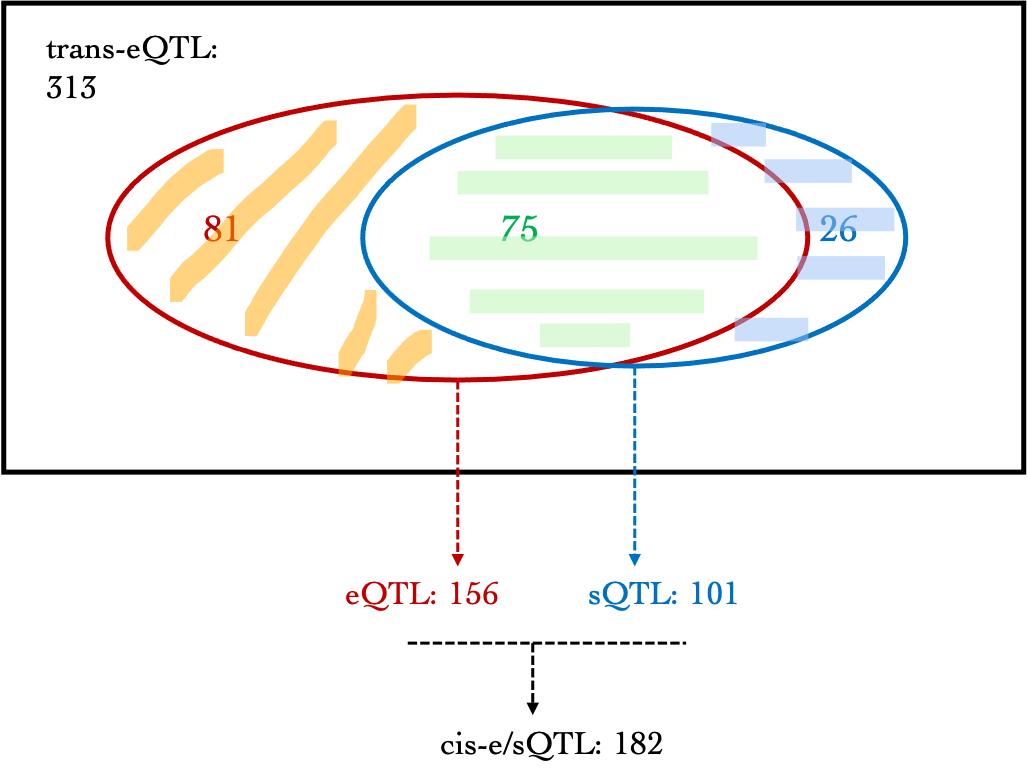
Are trans-eQTLs cis-e/sQTLs?

Past versions of 0526-1.png

Version	Author	Date
9275134	liliw-w	2021-07-08

Observations:

• For DGN, among 313 trans signals, 156 (~49.8%) are also cis-eQTLs, corresponding to 39 eGenes, including:

AC016753.7, BECN1, C17orf50, C2orf68, CFL2, CTD-2562J15.6, ERN1, FAM177A1, FIGNL1, FKRP, GGCX, HABP4, HSD17B1P1, ICAM2, KIAA0391, MAT2A, MLX, NEK6, NFE2, NFKBIA, OR2W3, PARP2, PEX12, PPP2R3C, PRKD2, PSMC3IP, RETSAT, RNF181, RP11-1094M14.8, RP11-69M1.4, RP11-85K15.2, SLC1A5, SLC2A3, SLFN12L, SYMPK, TMEM150A, TTC5, VAMP8, ZNF782

• For DGN, 101 (~32.3%) out of 313 trans signals are cis-sQTLs, corresponding to 71 introns. 26 trans-eQTLs are only sQTLs but not eQTLs. These signals are located on chromosome 15 and 19.

• Among 313 trans signals, 182 (~58.1%) are either cis-eQTLs or cis-sQTLs.

May 19

How many trans-eQTLs detected in DGN/GTEx whole blood are replicated in eQTLGen?

Replication of DGN signals in eQTLGen. Based on updated results, i.e. smaller and more gene modules & PCO\(_{\lambda>0.1}\).

Are trans-eQTLs cis-eQTLs?

1. Dataset: DGN

Dataset	#signal	is_ciseQTL(gene-based)	is_cissQTL(SNP-based)	is_cise(s)QTL(gene-based)
DGN	313	7	9	15
eQTLGen_DGN	784	17	30	45

Observations:

1.1 DGN

• Among 313 trans signals, 7 are also (gene-based) cis-eQTLs, corresponding to 5~7 independent SNPs. The cis-eGenes include SLC2A3, NFE2, KIAA0391, NFKBIA, ERN1, AC016753.7, MAT2A.

• Among 313 unique trans signals, 229 (~73%) have a neareset gene that are eGenes (with cis-eQTLs). Among 28 independent trans signals, 19 (~68%) have a neareset gene that are eGenes (with cis-eQTLs).

• Among 313 trans signals, 9 are also cis-sQTLs, corresponding to 6 independent SNPs.

1.2 eQTLGen_DGN

• Among 784 trans signals, 17 are also (gene-based) cis-eQTLs, corresponding to 9 independent SNPs. The cis-eGenes include AC016753.7, CPEB4, KIAA0391, MAT2A, MRFAP1, NFKBIA, PAQR6, PWP1, RNF181, RP11-539L10.2, RP11-69M1.4, S100P, SENP7, SLC25A44, SLC2A3, SMG5, TMEM79, ZNF782.

• Among 784 unique trans signals, 590 (~75%) have a neareset gene that are eGenes (with cis-eQTLs). Among 50 independent trans signals, 29 (~58%) have a neareset gene that are eGenes (with cis-eQTLs).

• Among 784 trans signals, 30 are also cis-sQTLs, corresponding to 10 independent SNPs.

2. Dataset: TCGA

3. eQTLGen?

March 8

Muscle

• Less modules, PCO\(_{\{\lambda: \lambda>0.1\}}\). 1 independent signal, large p.

• More modules, PCO\(_{\{\lambda: \lambda>0.1\}}\). 5 independent signal, small p.

• More modules, PCO\(_{\{\lambda: \lambda>1\}}\). 5 independent signal, relatively large p.

March 1

Real data analysis by PCO using more \(\lambda\)’s

Dataset: Muscle_Skeletal.

Fewer (independent) signals. \(PCO_{\{\lambda: \lambda>0.1\}}\) (1 signal) v.s. \(PCO_{\{\lambda: \lambda>1\}}\) (3 signals).

proteomics data

See the google doc here.

Other stuff

• RCC account storage

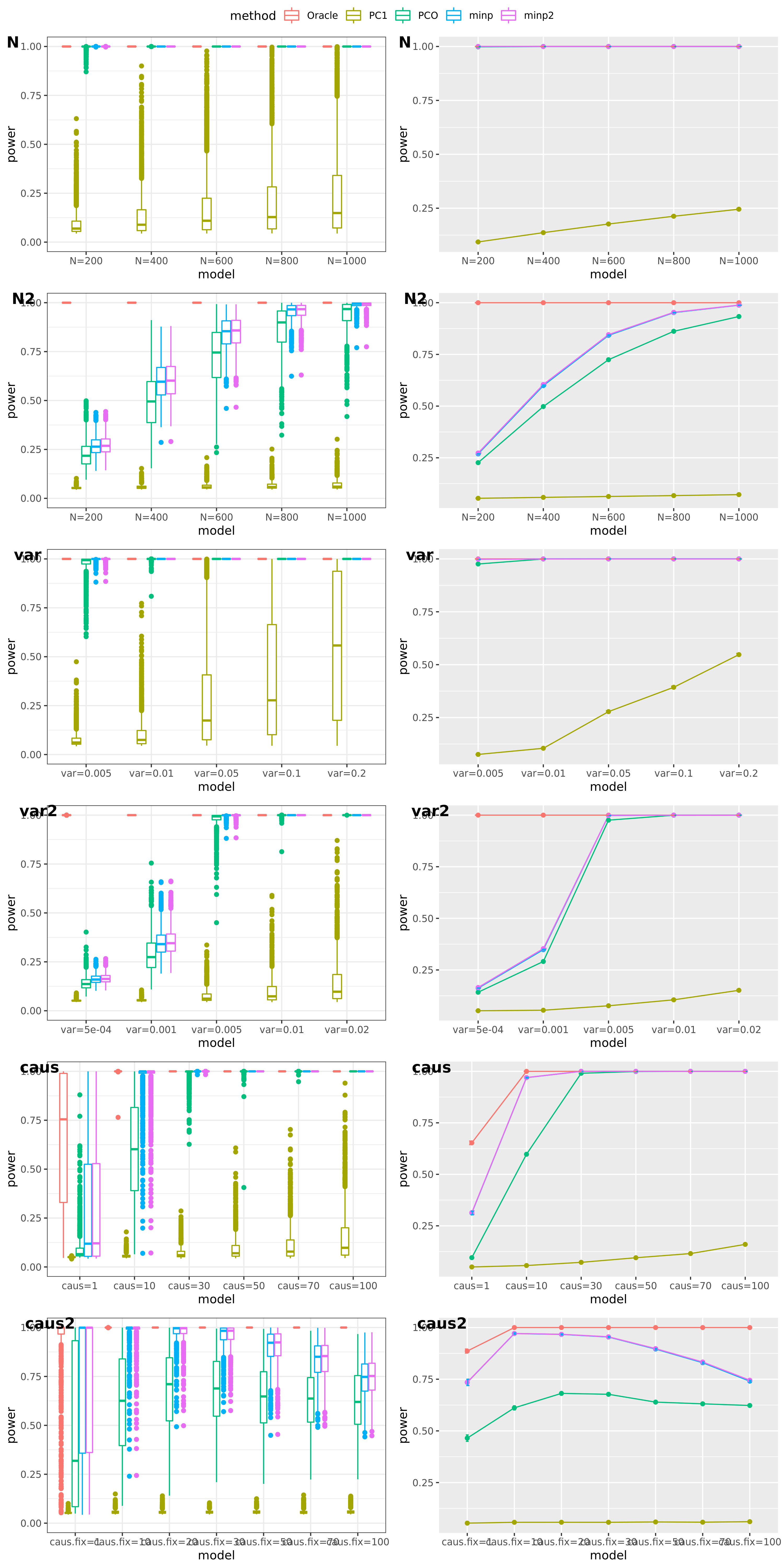
Feb 23

Updated simulation

1. Adjusted variance of effects

• tests

  • Oracle: \(\beta^T \Sigma^{-1}Z \approx \beta^T \hat\Sigma^{-1}Z = \beta^T (\sum_{\{\lambda_k: \lambda_k>0.1\}}\lambda_k u_k u_k^T) Z\)

  • PCO: Use \(\{\lambda_k: \lambda_k>0.1\}\).

• scenerios (\(K=100,K=105\))

  • N: var.b = 0.003; caus = 30%; N.seq = c(200, 400, 600, 800, 1000)

  • caus: var.b = 0.003; N = 500; caus.seq = c(1, 5, 10, 30, 50, 70, 100)

  • caus_fix: var.b.fix = 0.1; N = 500; caus.seq = c(1, 5, 10, 30, 50, 70, 100)

2. Run for other \(\Sigma\)’s. \(K=100,K=105\)

3. FDR level

The minimum null pvalue of PCO is \(\ge 10^{-9}\), similar as the significance threshold we use here \(10^{-9}\).

4. Results

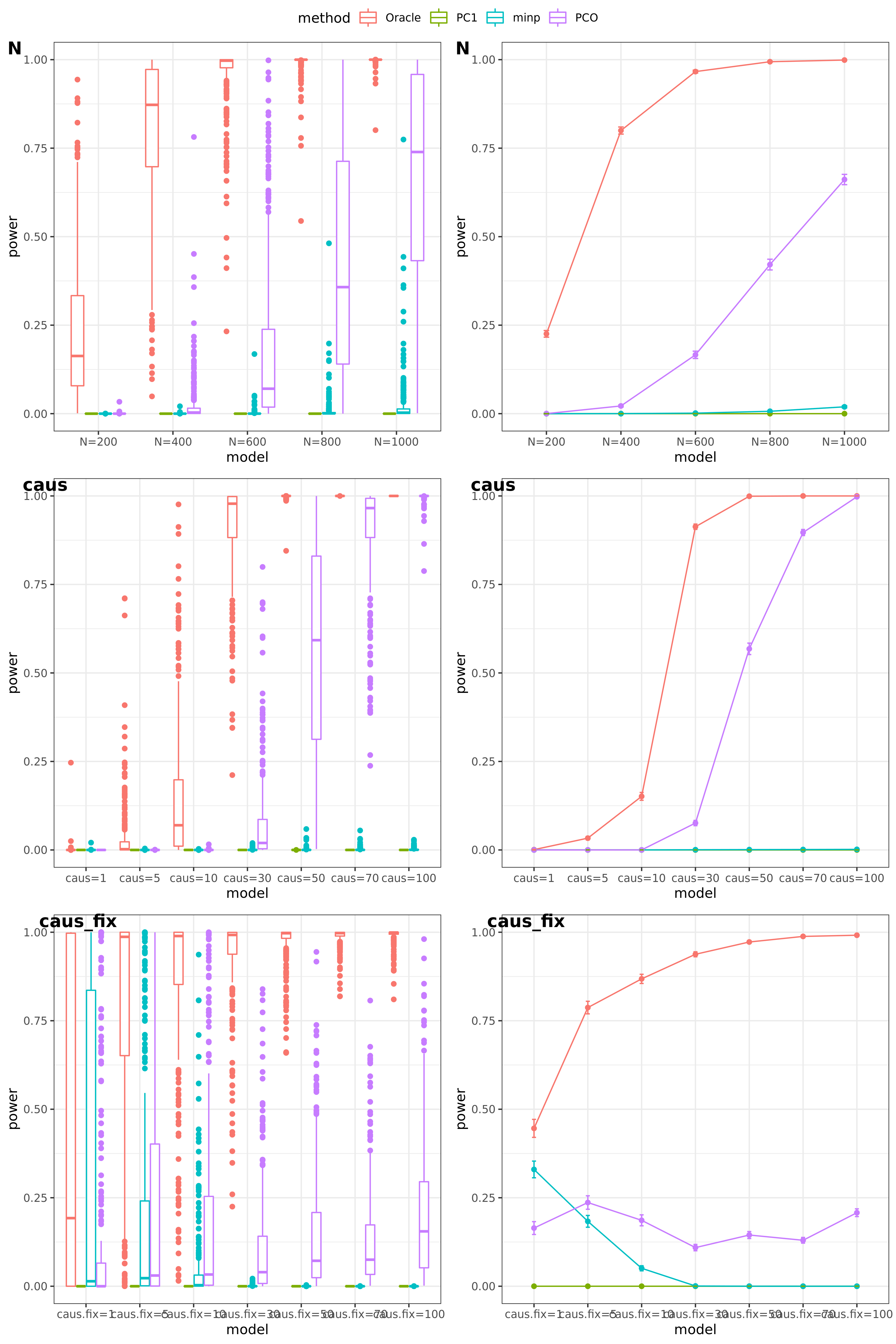
power under Bonferroni corretion cutoff

Past versions of 0223_power.lambda0.1.K100.png

Version	Author	Date
9275134	liliw-w	2021-07-08

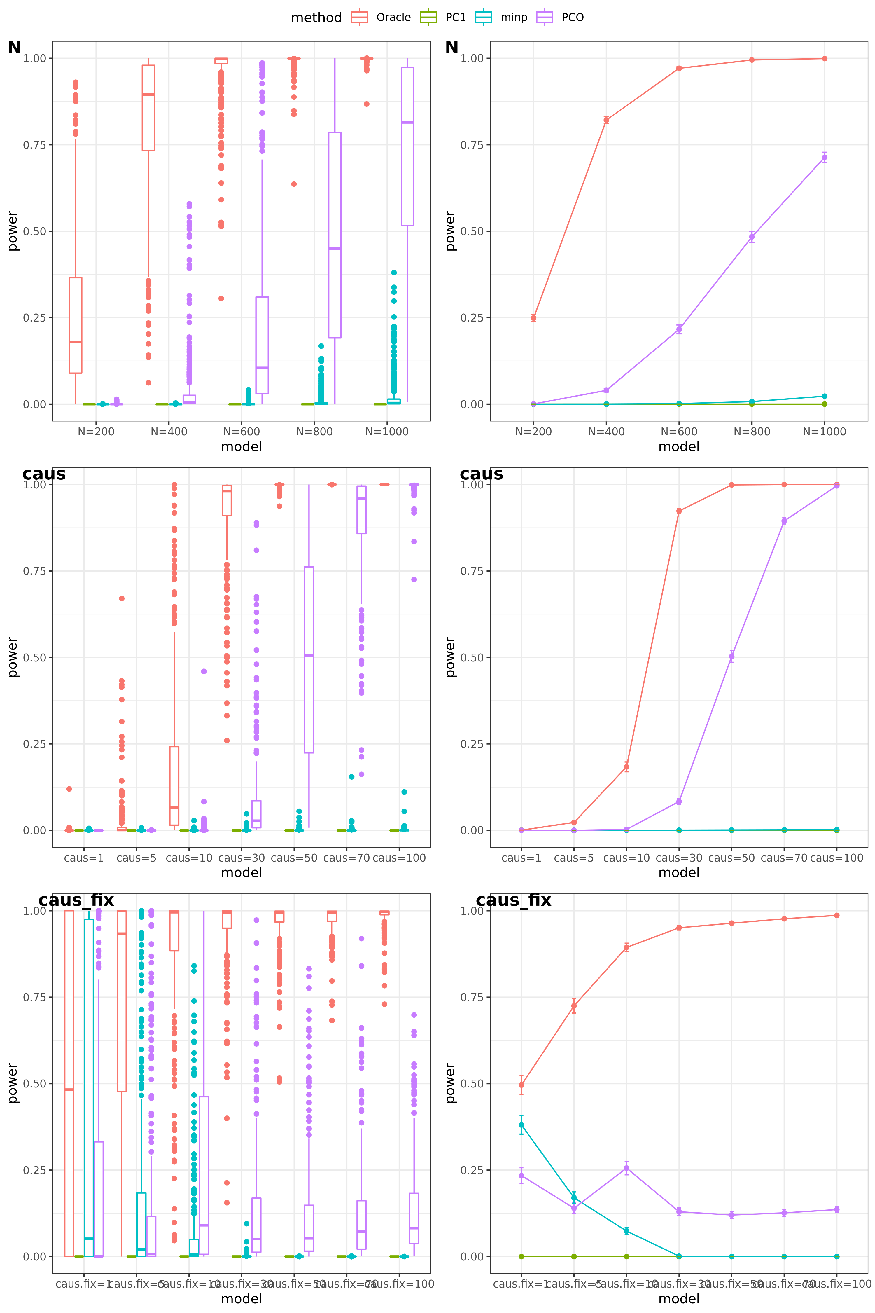
Another Sigma (K=105)

Past versions of 0223_power.lambda0.1.K105.png

Version	Author	Date
9275134	liliw-w	2021-07-08

Feb 16

simulation

• tests

  • Oracle: \(\beta^T \Sigma^{-1}Z \approx \beta^T \hat\Sigma^{-1}Z = \beta^T (\sum_{\{\lambda_k: \lambda_k>1\}}\lambda_k u_k u_k^T) Z\)

  • PC1;

  • minp = \(min\{p_1, \dots, p_K \} \times K\)

  • PCO: Use \(\{\lambda_k: \lambda_k>1\}\).

• Multiple testing

  The significance threshold is set based on the Bofferroni correction as the \(\frac{0.05}{50\times10^6} = 10^{-9}\) for univariate test and PC-based tests.

• scenerios (\(K=100\))

  • N: var.b = 0.01; caus = 100 (100%); N.seq = c(200, 400, 600, 800, 1000)

  • caus: var.b = 0.02; N = 500; caus.seq = c(1, 10, 30, 50, 70, 100)

  • caus_fix: var.b.fix = 0.2; N = 500; caus.seq = c(1, 10, 30, 50, 70, 100)

• results

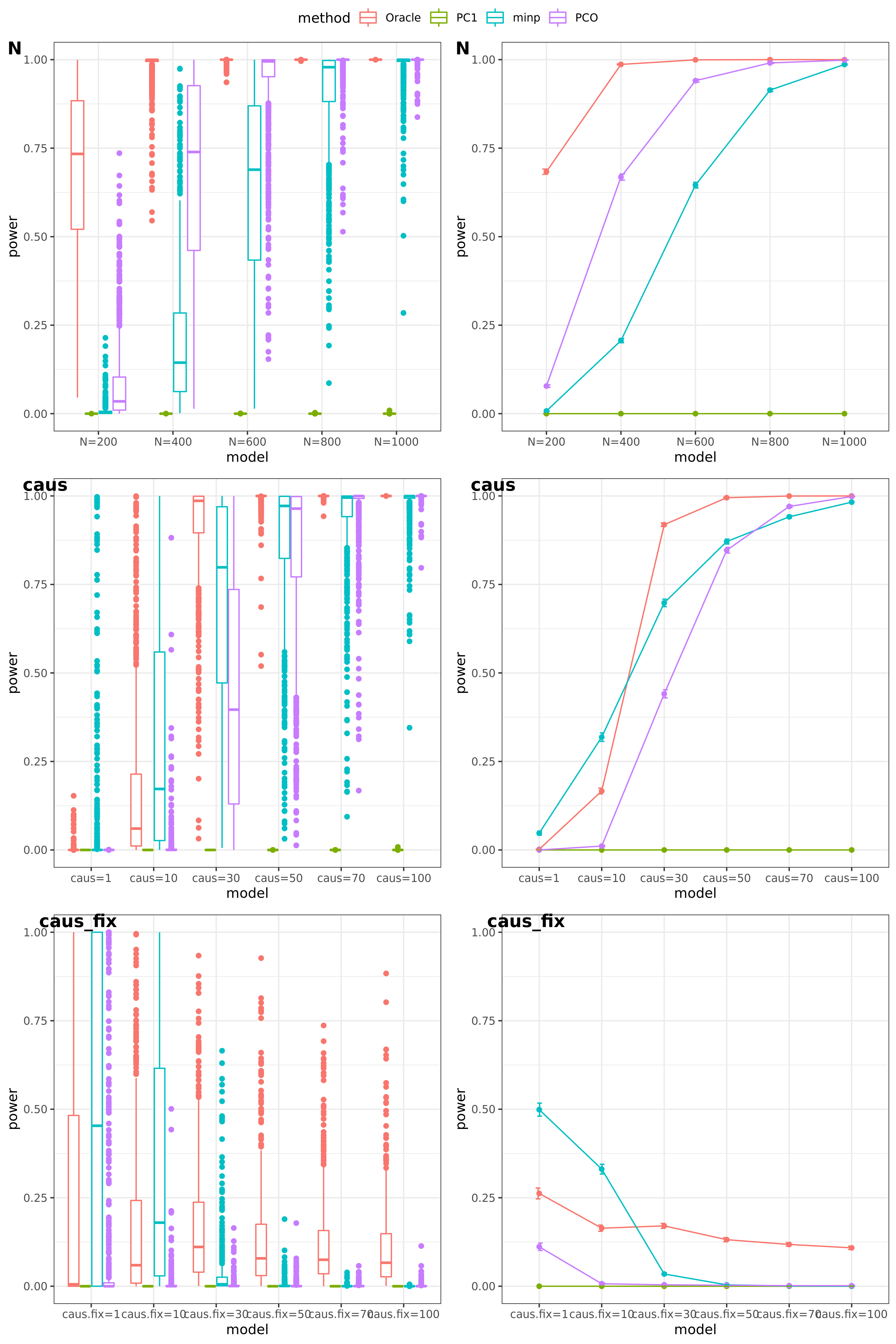
power under Bonferroni corretion cutoff

Past versions of 0216_power.lambda1.png

Version	Author	Date
9275134	liliw-w	2021-07-08

• Try other tests

  • Oracle: \(\beta^T \Sigma^{-1}Z \approx \beta^T \hat\Sigma^{-1}Z = \beta^T (\sum_{\{\lambda_k: \lambda_k>0.1\}}\lambda_k u_k u_k^T) Z\)

  • PCO: Use \(\{\lambda_k: \lambda_k>0.1\}\).

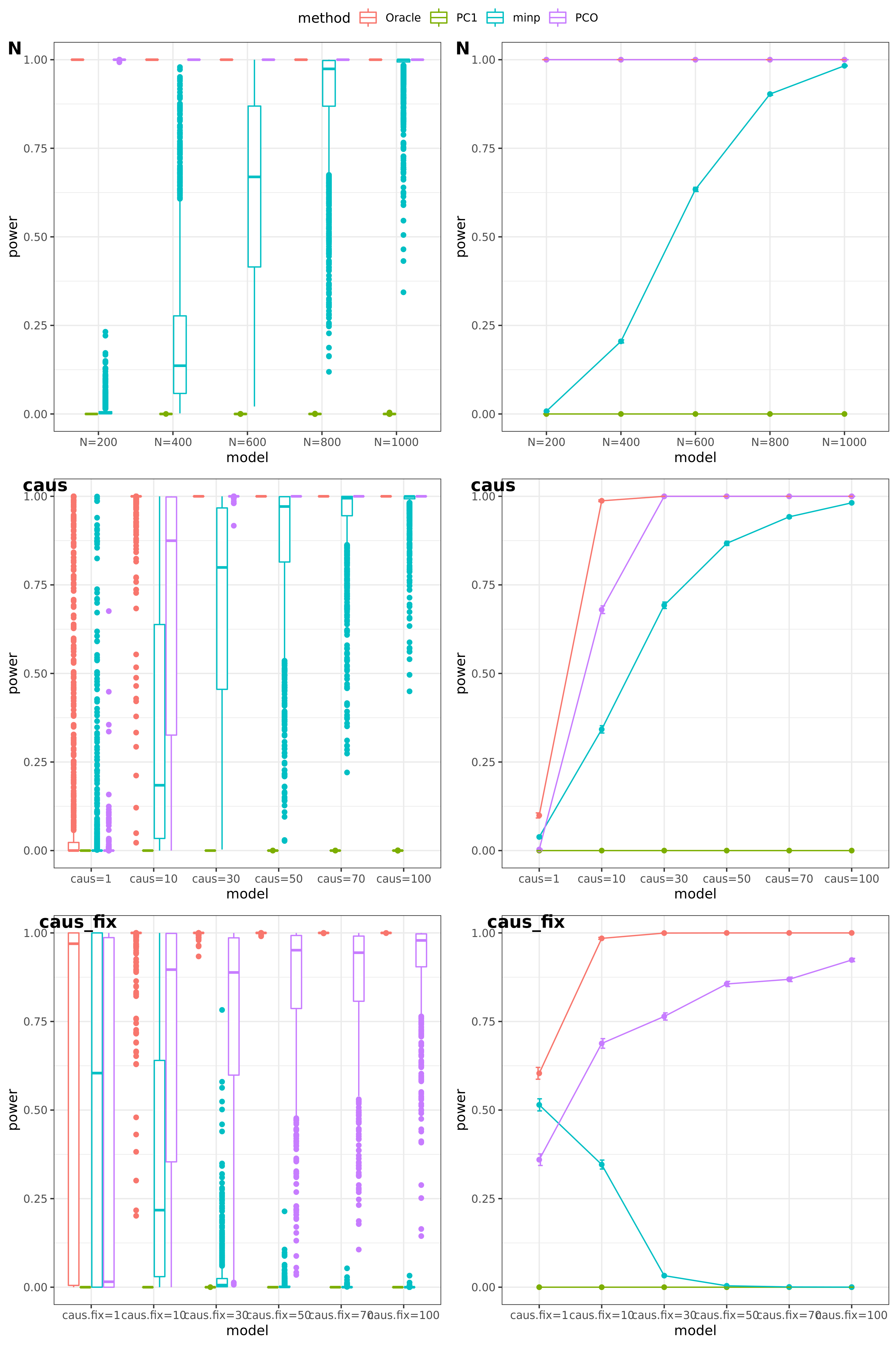
power under Bonferroni corretion cutoff

Past versions of 0216_power.lambda0.1.png

Version	Author	Date
9275134	liliw-w	2021-07-08

• For talk

(This figure should be updated as for the case of ‘u1’, the threshold is falsely set as 0.05, which should be \(10^{-9}\).)

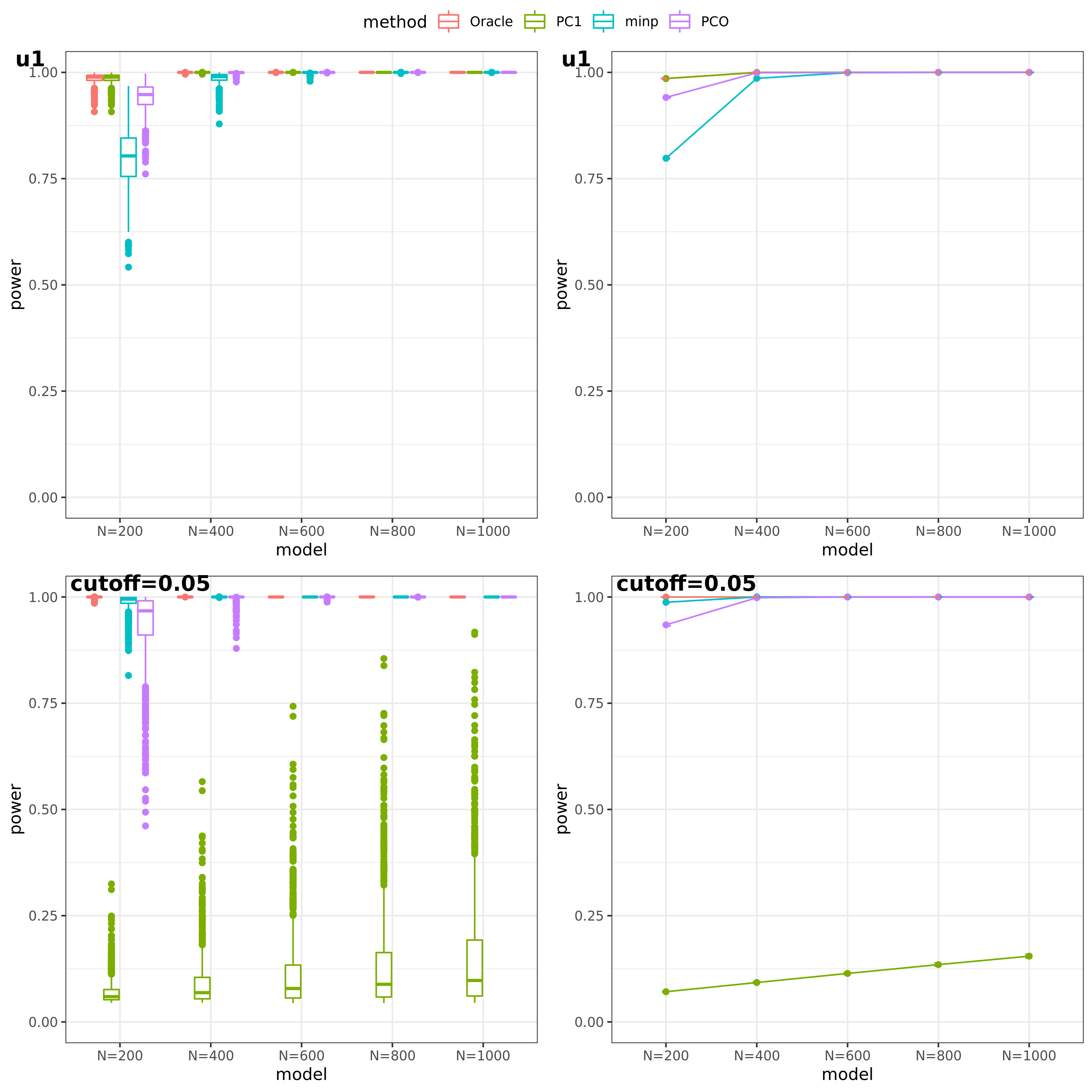
PC1 v.s. PCO

Past versions of 0216_talk.png

Version	Author	Date
9275134	liliw-w	2021-07-08

Jan 26

simulation

• Methods: Oracle, PC1, PCO, MinP, minp.

• Models: \(z \sim N(\sqrt{N} \beta, \Sigma)\). \(\beta \sim N(0, \sigma_{b}^2 I_{K \times K})\).

1. various sample size \(N\). 200, 400, 600, 800, 1000.

2. various \(\sigma_{b}^2\). 0.005, 0.01, 0.05, 0.1, 0.2.

3. various causality percentage. ???

• simulation.

  Generate \(10^4\) zscores under each model. \(10^4\) simulations.

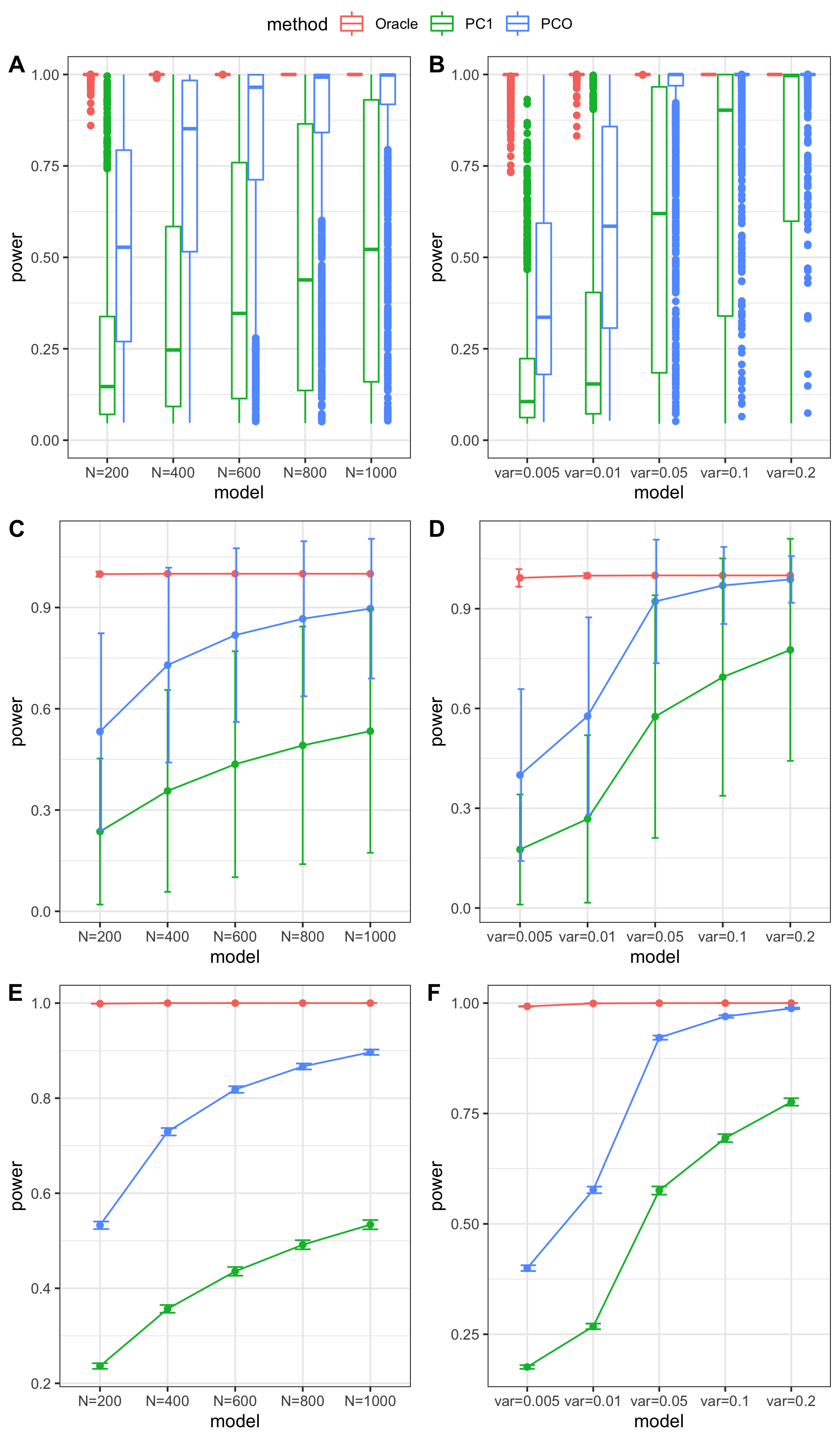
The following plot gives the boxplot, mean plot with standard deviation, and mean plot with standard error of the mean. Which one to use?

power under cutoff 0.05

Past versions of 0126_power_05.png

Version	Author	Date
9275134	liliw-w	2021-07-08

power comparison

Past versions of 0126_plot.error_bar.png

Version	Author	Date
9275134	liliw-w	2021-07-08

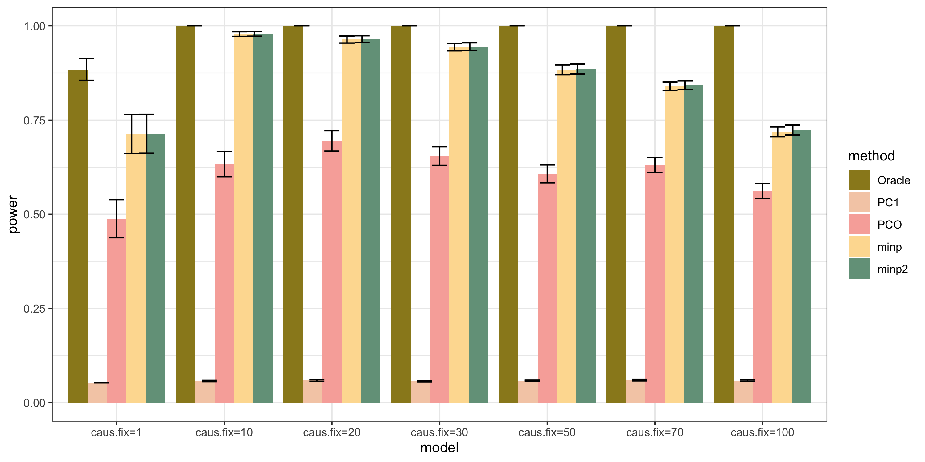
bar plot

Past versions of 0126_test.png

Version	Author	Date
9275134	liliw-w	2021-07-08

Larger FDR level, #signals in large and small module?

Here I will look at how the number of signals changes in the original large and current small modules when I increase the FDR level.

The plot below is based on Muscle tissue from GTEx_v8. The x-axis is for various FDR levels, including 5%, 10%, 15%, and 20%. The y-axis is for the number of signals under these FDR levels. I plot three types of signals, i.e. module and SNP pairs (left subplot), unique SNPs (middle subplot), independent SNPs (right subplot). The two colors represent our previous WGCNA modules (red) and current smaller WGCNA modules (blue).

We can observe (1) When increasing FDR levels, number of signals only increase a little bit, say 3-5 more signals. This means that the corrected pvalues are bipolar, i.e. either very small or very large. (2) Signals based on smaller modules are similar to that of previous standard modules.

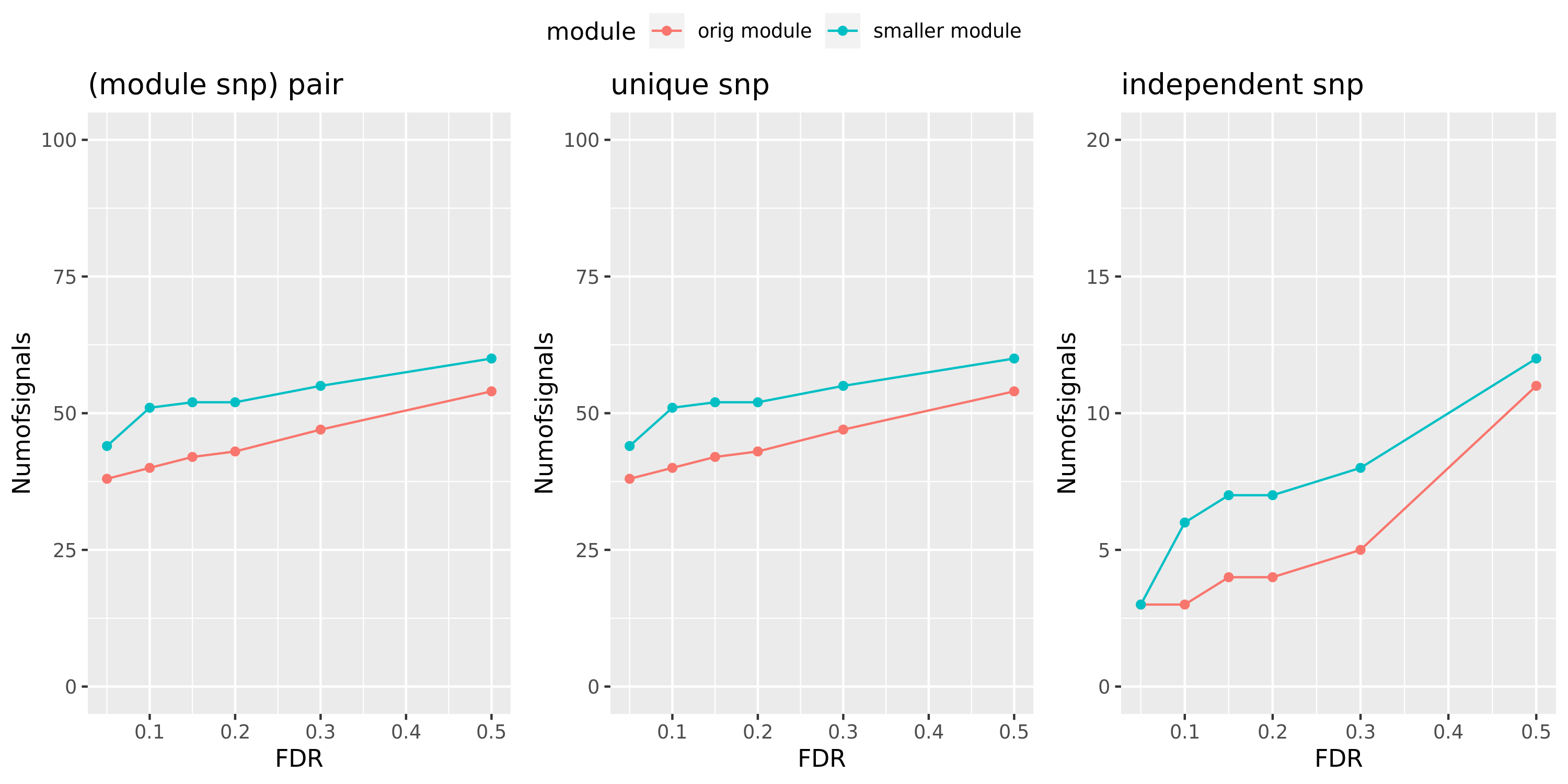
Muscle: #signals v.s.FDR

Past versions of 0126_signalsv.s.FDR.Muscle.png

Version	Author	Date
9275134	liliw-w	2021-07-08

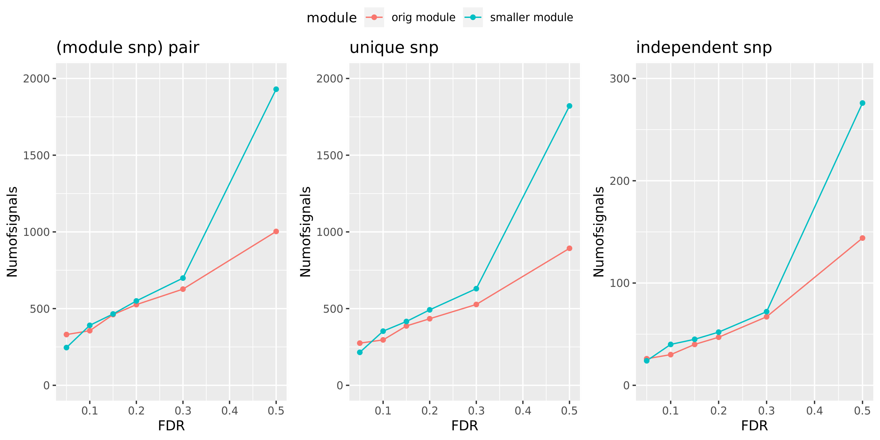
DGN: #signals v.s.FDR

Past versions of 0126_signalsv.s.FDR.DGN.png

Version	Author	Date
9275134	liliw-w	2021-07-08

Smaller gene modules, more signals?

I changed the parameter deepSplit in function cutreeDynamic from package WGCNA to get modules with smaller size. I run it on the Muscle tissue from GTEx (see GTEx_v8.Muscle_Skeletal.WGCNA in the GTEx results table). Compared to GTEx_v8.Muscle_Skeletal, though more modules (32 v.s. 18), they have same independent signals (3), located on chr5, chr10, and chr22.

The corresponding modules of these signals from small and large WGCNA share a large proportion of genes.

signal.Chr	module.small (#genes)	module.big (#genes)	#overlapped genes
chr5	module21 (89)	module15 (114)	88
chr10	module21 (89)	module15 (114)	88
chr22	module2 (297)	module4 (350)	257

The above table is for clusters obtained by method ‘WGCNA.min20_deep2’ (big) and ‘WGCNA.min20_deep4’ (small). Next, I give more info about the clusters by more methods, i.e. #genes in modules (A), #unclassfied genes (B), and #modules (C) by the six methods. I also give the pvalue distribution corresponding to these clusters below.

Generally, funcExplorer gives more modules, smaller module, and much more unclassified genes. Though the smaller modules, there aren’t many extreme pvalues. Say, the minimum p of all is about \(10^{-9}\), as compared to \(10^{-14}\) by other methods.

From the pvalue plot, it looks like ‘WGCNA.min10_deep4’ gives smaller clusters and some extreme pvalues. So next step I will run the whole pipleline for this setting.

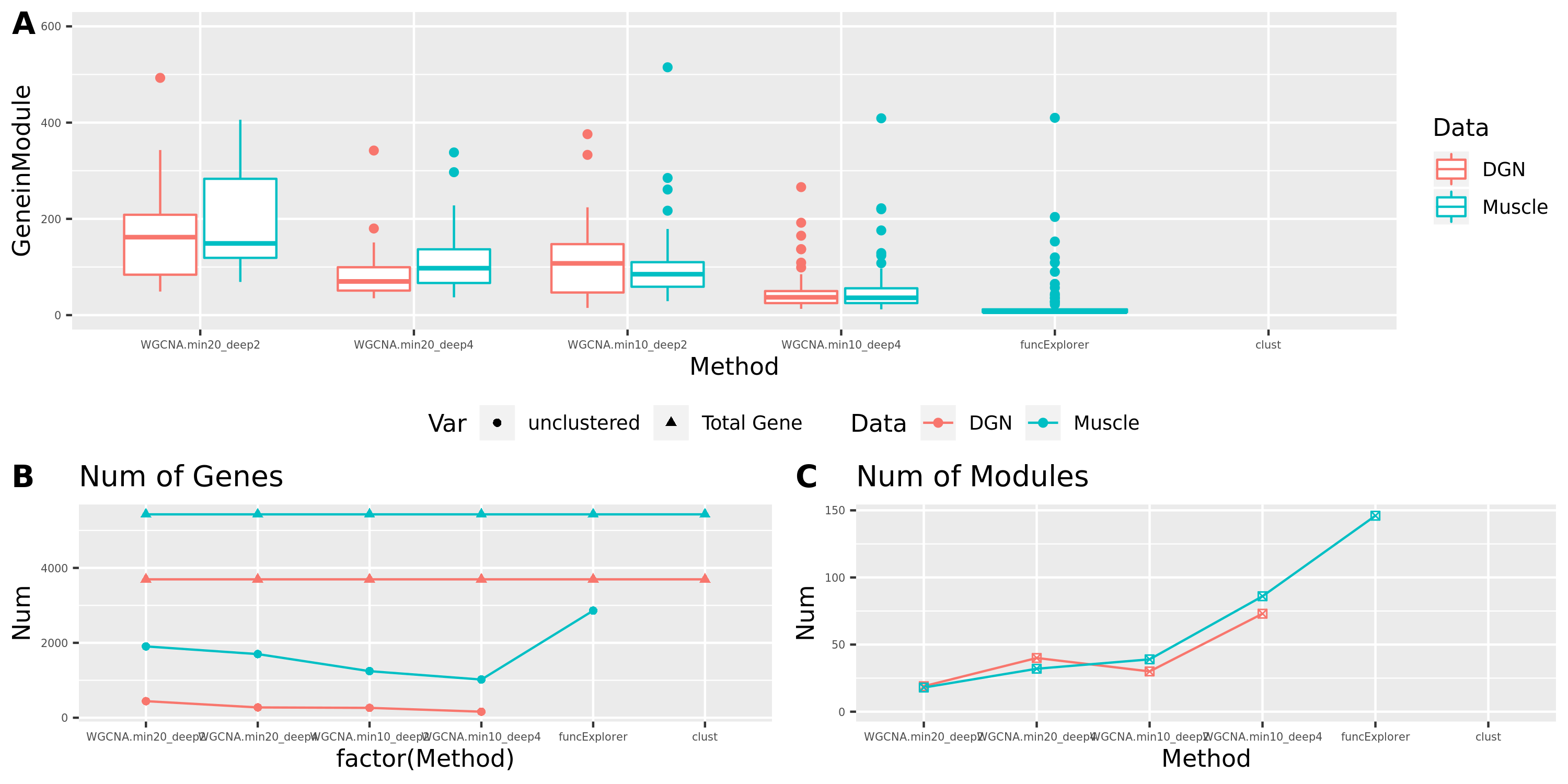
Modules v.s. methods/parameters

Past versions of 0126_modules.png

Version	Author	Date
9275134	liliw-w	2021-07-08

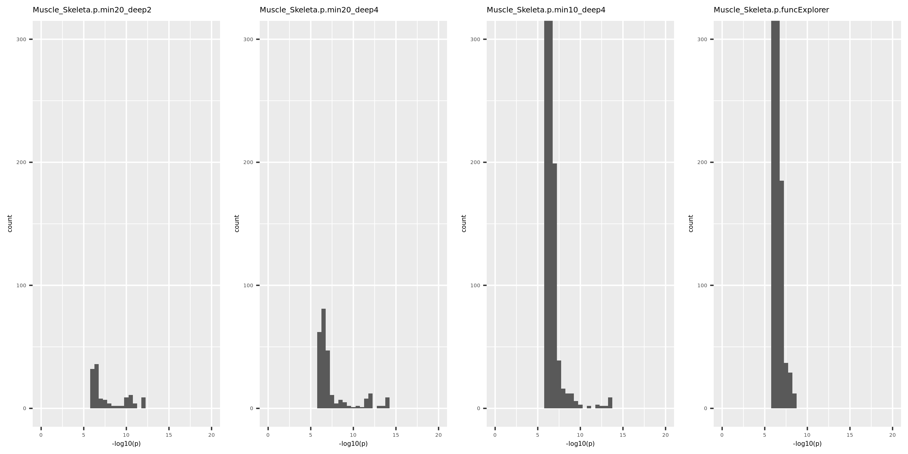
p distribution of Muscle

Past versions of 0126_Muscle_Skeleta.p.funcExplorer.png

Version	Author	Date
9275134	liliw-w	2021-07-08

Jan 05, Jan 19

Simulation

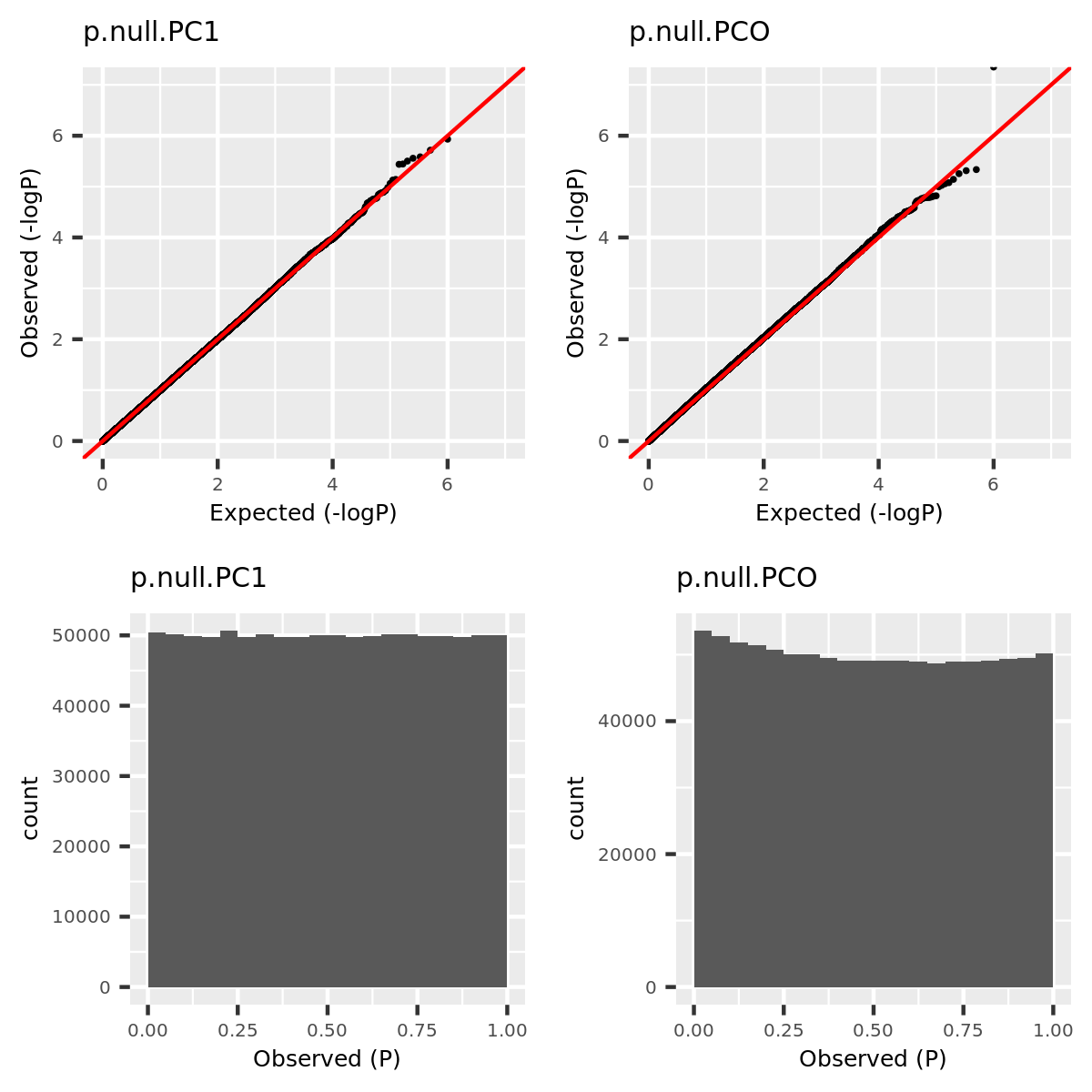
The simulations here aim to compare the power of PC-based tests including PC1 (using only the primary PC) and PCO (using combined PC’s), and non-PC based test MinP. The simulations consist of two parts: (1) verify that type 1 error is well controlled; (2) compare power of tests. At this time, I simply assume there is no LD among SNPs, i.e. tests are independent.

1. Verify that type 1 error is well controlled.

Since the tests are assumed to be independent, the null pvalues should be uniformly distributed. To verify that, I estimate the null pvalues by empirical p’s obtained from the following steps.

Step1. Generate \(z_0 \sim N(0, \Sigma) | H_0\).

Step2. Run tests including PC1, PCO, MinP for \(10^6\) times and obtain \(10^6\) p’s for each test.

Step3. Compute the empirical T1E at significance \(\alpha\) by \(\frac{I\{p<\alpha\}}{10^6}\). Draw qqplot of \(-log_{10}p\).

The correlation matrix \(\Sigma\) is the correlation of genes in module15 of GTEx dataset Muscle_Skeletal (Sigma.Muscle_Skeletal.module15.chr7.rds).

alpha	PC1	PCO	MinP
5e-02	0.050356	0.053584
1e-04	0.000093	0.000114

qqplot.simulation.null

Past versions of 0119_qqplot.simulation.null.png

Version	Author	Date
9275134	liliw-w	2021-07-08

2. Compare power of tests.

To compare the power of non-/PC-based tests, I will run the oracle test in addition to PC1, PCO, and MinP to benchmark the power. It’s mentioned in the PCO paper that given a fixed correlation relationship among the phenotypes, the power of a test depends on the relationship bewteen the true effects (\(\beta\)) and the phenotype correlation (\(\Sigma\)). Therefore, to see which tests perform well in what cases, I will consider different models, including (1) \(\beta=10 u_1\); (2) \(\beta=4 u_k\); (3) \(\beta=1.5 u_K\); (4) \(\beta=rnorm(K)\); (5) \(\beta=rnorm(0.7K)\); (6) \(\beta=rnorm(0.3K)\).

Step1. Generate \(z_0 \sim N(\beta, \Sigma) | H_1\).

Step2. Run tests including Oracle, PC1, PCO, MinP for \(10^6\) times and obtain \(10^6\) p’s for each test.

Step3. Compute the power at significance \(\alpha\) by \(\frac{I\{p<\alpha\}}{10^6}\).

Model	Oracle	PC1	PCO	MinP
u1	0.946341	0.902540	0.746301
uPCO	0.989835	0.050178	0.713434
uK	0.953727	0.049719	0.054140
100%	1.000000	0.058867	0.945918
70%	1.000000	0.058910	0.580368
30%	0.999995	0.050201	0.149904

GTEx

Results

The table below summarizes all results I have so far, followed by figures of the distributions of pvalues in various datasets.

Dataset	Nsample	All	Annotated	Filtered	Filtered_info	Final	Nmodule	FDR	Nperm	QTL_Module	unique_QTL	independent_QTL
DGN	913	13634	11979	8120	0;165;1663;8073	3859	21	combined chr+module	20	659	623	40
DGN_new	913	13634	12585	9939	1;453;1798;8705	3695	19	combined chr+module	10	331	275	26
TCGA	788	17656	15994	12694	336;3504;10697;598	4962
GTEx_v8.Whole_Blood	670	20315	20315	15245	619;4544;3677;13096	5070	22	combined chr+module	10	4	4	2
GTEx_v8.Muscle_Skeletal	706	21031	21031	15601	675;4447;3631;13490	5430	18	combined chr+module	10	38	38	3
GTEx_v8.Skin_Sun_Exposed_Lower_leg	605	25196	25196	18801	807;6458;4557;15650	6395	30	combined chr+module	10	1	1	1
GTEx_v8.Artery_Tibial	584	23304	23304	17390	795;5588;4202;14730	5914	20	combined chr+module	10	0	0	0
GTEx_v8.Muscle_Skeletal.cross	706	21031	21031	7141	675;4447;3631;0	13890	39	combined chr+module	10	43	43	4
GTEx_v8.Muscle_Skeletal.WGCNA	706	21031	21031	15601	675;4447;3631;13490	5430	32	combined chr+module	10	44	44	3
DGN_new.WGCNA	913	13634	12585	9939	1;453;1798;8705	3695	40	combined chr+module	10
TCGA_new

DGN

Past versions of 0119_DGN.p.png

Version	Author	Date
9275134	liliw-w	2021-07-08

DGN_new

Past versions of 0119_DGN_new.p.png

Version	Author	Date
9275134	liliw-w	2021-07-08

Whole_Blood

Past versions of 0119_Whole_Blood.p.png

Version	Author	Date
9275134	liliw-w	2021-07-08

Muscle_Skeletal

Past versions of 0119_Muscle_Skeletal.p.png

Version	Author	Date
9275134	liliw-w	2021-07-08

Skin_Sun_Exposed_Lower_leg

Past versions of 0119_Skin_Sun_Exposed_Lower_leg.p.png

Version	Author	Date
9275134	liliw-w	2021-07-08

Artery_Tibial

Past versions of 0119_Artery_Tibial.p.png

Version	Author	Date
9275134	liliw-w	2021-07-08

Muscle_Skeletal.cross

Past versions of 0119_Muscle_Skeletal.cross.p.png

Version	Author	Date
9275134	liliw-w	2021-07-08

Remarks

1. The dataset “DGN_new” represents DGN through the standard filtering (see “Gene filter” on Dec 10).

2. GTEx datasets generally have few significant signals and relatively large pvalues (compared to DGN).

3. The dataset “GTEx_v8.Muscle_Skeletal.cross” uses Muscle_Skeletal samples from GTEx_v8 (similar as GTEx_v8.Muscle_Skeletal), but without removing cross-mapped genes before constructing gene modules. Therefore, there are 13890 genes (v.s. 5430 in GTEx_v8.Muscle_Skeletal) in total which result in 39 modules (v.s. 18 in GTEx_v8.Muscle_Skeletal). We do this step because we observed that there are relatively few signals using our original pipeline and we wonder if the reason to this observation is us filtering too many genes in the first step and leaving too few signals. To check on this, we put the “filtering” to the last step, i.e. including potentially cross-mapped genes into the analysis and generate significant variant-module pairs. We then exclude those where target eGene in the module is cross-mappable with any gene within 1Mb of the variant. Hopefully we could have more signals.

   However, though the increased genes and modules, the number of identified signals (43) is similar as that using the original pipeline (38). Next, I will look into these signals.

GTEx_v8.Muscle_Skeletal

variant-module	p	q
module15:10:48930105	8.63e-10	8.33e-03
module15:5:132440814	1.56e-09	2.16e-02
module15:5:132448891	3.36e-09	4.74e-02
module15:5:132450078	5.81e-12	0.00e+00
module15:5:132450726	5.96e-12	0.00e+00
module15:5:132450916	8.89e-12	0.00e+00
module15:5:132451361	5.97e-11	0.00e+00
module15:5:132451586	1.11e-11	0.00e+00
module15:5:132453865	1.05e-12	0.00e+00
module15:5:132454053	9.94e-13	0.00e+00
module15:5:132454171	1.03e-12	0.00e+00
module15:5:132454631	1.44e-12	0.00e+00
module15:5:132454724	1.08e-12	0.00e+00
module15:5:132455672	1.07e-12	0.00e+00
module15:5:132455979	1.04e-12	0.00e+00
module15:5:132456154	9.96e-13	0.00e+00
module15:5:132456710	6.04e-11	0.00e+00
module15:5:132458606	5.33e-11	0.00e+00
module15:5:132459905	4.84e-11	0.00e+00
module15:5:132459971	5.04e-11	0.00e+00
module15:5:132460190	5.05e-11	0.00e+00
module15:5:132460375	5.56e-11	0.00e+00
module15:5:132460917	5.03e-11	0.00e+00
module15:5:132461111	5.17e-11	0.00e+00
module15:5:132463834	5.47e-11	0.00e+00
module15:5:132464413	3.90e-11	0.00e+00
module15:5:132464907	1.01e-12	0.00e+00
module15:5:132466034	4.56e-11	0.00e+00
module15:5:132468333	1.32e-10	0.00e+00
module15:5:132468353	5.74e-11	0.00e+00
module15:5:132468564	8.53e-11	0.00e+00
module15:5:132469724	5.63e-11	0.00e+00
module15:5:132469899	6.96e-11	0.00e+00
module15:5:132470043	1.03e-10	0.00e+00
module15:5:132470796	5.42e-11	0.00e+00
module15:5:132471932	8.01e-11	0.00e+00
module15:5:132474927	2.71e-10	2.94e-03
module4:22:23508295	3.76e-10	5.71e-03

GTEx_v8.Muscle_Skeletal.cross

variant-module	p	q
module8:1:123955560	9.97e-12	0.00e+00
module8:1:123955561	1.06e-11	0.00e+00
module8:16:36353041	3.49e-11	6.67e-03
module8:16:36353056	8.29e-11	1.25e-02
module8:5:132453865	1.56e-09	3.12e-02
module8:5:132454053	1.59e-09	2.86e-02
module8:5:132454171	1.52e-09	3.33e-02
module8:5:132454631	1.43e-09	3.57e-02
module8:5:132454724	1.53e-09	3.23e-02
module8:5:132455672	1.50e-09	3.45e-02
module8:5:132455979	1.56e-09	3.03e-02
module8:5:132456154	1.78e-09	3.42e-02
module8:5:132456710	1.36e-09	3.33e-02
module8:5:132458606	3.37e-10	1.76e-02
module8:5:132459905	6.50e-10	1.74e-02
module8:5:132459971	3.92e-10	1.43e-02
module8:5:132460190	3.50e-10	1.58e-02
module8:5:132460375	3.37e-10	1.67e-02
module8:5:132460917	3.98e-10	1.36e-02
module8:5:132461111	3.57e-10	1.50e-02
module8:5:132463834	8.21e-10	2.40e-02
module8:5:132464413	9.93e-10	2.69e-02
module8:5:132466034	6.75e-10	1.67e-02
module8:5:132468333	1.86e-09	3.50e-02
module8:5:132468353	1.69e-09	3.06e-02
module8:5:132468564	2.43e-09	4.19e-02
module8:5:132469724	1.93e-09	3.66e-02
module8:5:132469899	1.73e-09	3.24e-02
module8:5:132470043	1.56e-09	2.94e-02
module8:5:132470796	1.85e-09	3.33e-02
module8:5:132471932	2.37e-09	4.29e-02
module8:5:46659000	9.86e-13	0.00e+00
module8:5:46906585	2.34e-11	7.14e-03
module8:5:47027928	0.00e+00	0.00e+00
module8:5:47068540	0.00e+00	0.00e+00
module8:5:47166316	3.33e-16	0.00e+00
module8:5:47210790	0.00e+00	0.00e+00
module8:5:47210990	0.00e+00	0.00e+00
module8:5:47258679	4.44e-16	0.00e+00
module8:5:47258917	3.33e-16	0.00e+00
module8:5:49809727	2.70e-13	0.00e+00
module8:5:49930686	0.00e+00	0.00e+00
module8:5:49936394	1.10e-11	0.00e+00

For GTEx_v8.Muscle_Skeletal, there are 38 variant-module pairs, corresponding to 2 module (module 15, module4) and 3 independent loci on (chr5, chr10, chr22). GTEx_v8.Muscle_Skeletal.cross has 43 variant-module pairs, corresponding to 1 module (module 8) and 4 independent loci on (chr1, chr5, chr16).

The signal on chr5 is significant for both module 15 (114 genes) and module 8 (394 genes) in two datasets, which have 82 shared genes. Take SNP [rs2706381][rs2706381 GTEx ref] (chr5:132474927) for example. It is ["in cis with IRF1 ($P \le 2\times10^{-10}$; Fig. 6c), a transcription factor that facilitates regulation of the interferon-induced immune response"][rs2706381 GTEx ref]. It is also ["associated in trans with PSME1 ($P \le 1.1\times10^{-11}$) and PARP10 ($P \le 7.8\times10^{-10}$)"][rs2706381 GTEx ref]. These two genes are included in module 15. The reference also gives additional results to "suggest that cis-regulatory loci affecting IRF1 are regulators of interferon-responsive inflammatory processes involving genes including PSME1 and PARP10, with implications for complex traits specific to muscle tissue".

I also looked at the enrichment of the genes in module 15. These genes are mainly enriched in immunity-related terms and tuberculosis. To reproduce, use the gene list [here](asset/0119_gene.GTEx_v8.Muscle_Skeletal.module15.txt).

SNP 10:48930105. module 15.

module4:22:23508295

+ Check if the signals' nearby genes are cross-mapped with genes in their corresponding module. The signal on chr5 corresponding to module8 has 20 genes +/- 500Kb away from its TSS. Many of them are crosspable with genes in the module 8. The number of of genes in the module crossmapped with each of the 20 genes are: `1, 144, 0, 62, 54, 0, 63, 4, 0, 0, 0, 59, 145, 0, 0, 128, 0, 23, 53`, where the nearest gene is crossmappable with 1 gene in the module.

• The other signals on chr1, chr16, and chr5:47210790 don’t have any nearby genes around its TSS.

• See the following plot for number of cross-mapped genes in each module.

Past versions of 0119_nCross.png

Version	Author	Date
9275134	liliw-w	2021-07-08

New TCGA by the standard filtering

eQTLGen

1. eQTLGen description

   This full dataset includes 19942 genes that showed expression in blood tested and 10317 SNPs that are trait-associated SNPs based on GWAS Catalog.

   After gene filter steps described in Dec 10, there are 4963 genes left. Applying the same filtering to 13634 DGN genes, there are 3695 genes left, among which 3642 are also included in eQTLGen. So, I will use these genes to do the downstream analysis, e.g. constructing co-expressed gene modules. These 3642 genes result in 19 gene modules.

2. Replication of DGN signals in eQTLGen

   The table below gives the signals found in eQTLGen and DGN.

   The first two rows give results based on eQTLGen zscores, with row 1 using qvalue for FDR correction (threshold \(0.05\)) and row 2 using \(\frac{0.05}{\#DGN signals}\) as significance threshold. The third row is based on the same gene modules and SNPs but tensorQTL zscores using DGN expression data. The FDR correction uses the empirical distribution of pvalues from the combined chr’s and modules (10 permutations).

Dataset	FDR	minp	(QTL, module)	unique QTL	independent QTL
eQTLGen	qvalue	5.82e-04	2195	909	348
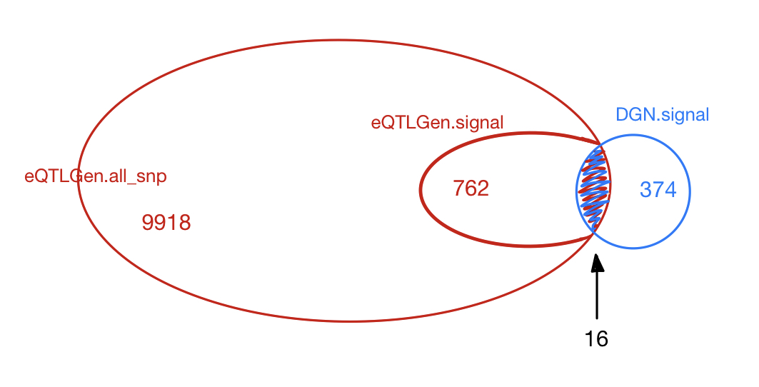
eQTLGen	0.05/#DGN signals	1.18e-04	1707	762	286
eQTLGen_DGN	combined chr+module #10-perms	1.00e-07	420	374	28

Among 374 eQTLGen_DGN signals, 16 are replicated in 762 eQTLGen signals. These 16 replicated signals consists of 6 independent SNPs, including (based on GRCh37),

• rs12485738 : 3:56865776, intron variant of ARHGEF3.
• rs643381 : 6:139839423. (rs590856, 6:139844429).
• rs149007767 7:50370254: , intron variant of IKZF1.
• rs12718597 : 7:50428428, intron variant of IKZF1.
• rs35979828 : 12:54685880, 500B downstream variant of NFE2.
• rs7210990 : 17:16170764, intron variant of PIGL.

3. Replication of DGN signals in eQTLGen

DGN

Past versions of 0119_eQTLGen_DGN_venn.jpeg

Version	Author	Date
9275134	liliw-w	2021-07-08

Session information

R version 4.1.0 (2021-05-18)
Platform: x86_64-apple-darwin17.0 (64-bit)
Running under: macOS Catalina 10.15.7

Matrix products: default
BLAS:   /Library/Frameworks/R.framework/Versions/4.1/Resources/lib/libRblas.dylib
LAPACK: /Library/Frameworks/R.framework/Versions/4.1/Resources/lib/libRlapack.dylib

locale:
[1] en_US.UTF-8/en_US.UTF-8/en_US.UTF-8/C/en_US.UTF-8/en_US.UTF-8

attached base packages:
[1] stats     graphics  grDevices utils     datasets  methods   base     

other attached packages:
[1] data.table_1.14.0 workflowr_1.6.2  

loaded via a namespace (and not attached):
 [1] Rcpp_1.0.6        whisker_0.4       knitr_1.33        magrittr_2.0.1   
 [5] R6_2.5.0          rlang_0.4.11      fansi_0.5.0       highr_0.9        
 [9] stringr_1.4.0     tools_4.1.0       xfun_0.23         utf8_1.2.1       
[13] git2r_0.28.0      htmltools_0.5.1.1 ellipsis_0.3.2    rprojroot_2.0.2  
[17] yaml_2.2.1        digest_0.6.27     tibble_3.1.2      lifecycle_1.0.0  
[21] crayon_1.4.1      later_1.2.0       vctrs_0.3.8       promises_1.2.0.1 
[25] fs_1.5.0          glue_1.4.2        evaluate_0.14     rmarkdown_2.10   
[29] stringi_1.6.2     compiler_4.1.0    pillar_1.6.1      httpuv_1.6.1     
[33] pkgconfig_2.0.3