Data wrangling for Class Project
Maggie Douglas
2026-02-14
Last updated: 2026-02-27
Checks: 6 1
Knit directory: dickinson_power/
This reproducible R Markdown analysis was created with workflowr (version 1.7.1). The Checks tab describes the reproducibility checks that were applied when the results were created. The Past versions tab lists the development history.
The R Markdown file has unstaged changes. To know which version of
the R Markdown file created these results, you’ll want to first commit
it to the Git repo. If you’re still working on the analysis, you can
ignore this warning. When you’re finished, you can run
wflow_publish to commit the R Markdown file and build the
HTML.
Great job! The global environment was empty. Objects defined in the global environment can affect the analysis in your R Markdown file in unknown ways. For reproduciblity it’s best to always run the code in an empty environment.
The command set.seed(20260107) was run prior to running
the code in the R Markdown file. Setting a seed ensures that any results
that rely on randomness, e.g. subsampling or permutations, are
reproducible.
Great job! Recording the operating system, R version, and package versions is critical for reproducibility.
Nice! There were no cached chunks for this analysis, so you can be confident that you successfully produced the results during this run.
Great job! Using relative paths to the files within your workflowr project makes it easier to run your code on other machines.
Great! You are using Git for version control. Tracking code development and connecting the code version to the results is critical for reproducibility.
The results in this page were generated with repository version e752845. See the Past versions tab to see a history of the changes made to the R Markdown and HTML files.
Note that you need to be careful to ensure that all relevant files for
the analysis have been committed to Git prior to generating the results
(you can use wflow_publish or
wflow_git_commit). workflowr only checks the R Markdown
file, but you know if there are other scripts or data files that it
depends on. Below is the status of the Git repository when the results
were generated:
Ignored files:
    Ignored:    .DS_Store
    Ignored:    .Rhistory
    Ignored:    .Rproj.user/
    Ignored:    data/.DS_Store
    Ignored:    data/FY25 Main Meter Data.xlsx
    Ignored:    data/building_list_FY25_updated.xlsx
    Ignored:    data/graph_data_life_exp.csv
    Ignored:    keys/.DS_Store
    Ignored:    output/building_check.csv
    Ignored:    output/building_check.xlsx
    Ignored:    output/kwh_annual.csv
    Ignored:    output/kwh_annual_20260225.csv
    Ignored:    output/kwh_annual_20260226.csv
    Ignored:    output/kwh_daily.csv
    Ignored:    output/kwh_daily_20260225.csv
    Ignored:    output/kwh_daily_20260226.csv
    Ignored:    output/kwh_main_annual.csv
    Ignored:    output/kwh_main_daily.csv

Unstaged changes:
    Modified:   analysis/data_wrangling_final.Rmd

Staged changes:
    Deleted:    keys/~$fy25_building_list_updated.xlsx
Note that any generated files, e.g. HTML, png, CSS, etc., are not included in this status report because it is ok for generated content to have uncommitted changes.
These are the previous versions of the repository in which changes were
made to the R Markdown (analysis/data_wrangling_final.Rmd)
and HTML (docs/data_wrangling_final.html) files. If you’ve
configured a remote Git repository (see ?wflow_git_remote),
click on the hyperlinks in the table below to view the files as they
were in that past version.
| File | Version | Author | Date | Message |
|---|---|---|---|---|
| Rmd | e752845 | maggiedouglas | 2026-02-26 | adjust data processing + building summary |
| html | e752845 | maggiedouglas | 2026-02-26 | adjust data processing + building summary |
| Rmd | 08cd7e1 | maggiedouglas | 2026-02-25 | update wrangling script |
| html | 08cd7e1 | maggiedouglas | 2026-02-25 | update wrangling script |
| Rmd | 8c6712f | maggiedouglas | 2026-02-24 | update script to fix issues |
| html | 8c6712f | maggiedouglas | 2026-02-24 | update script to fix issues |
| Rmd | 2fef649 | maggiedouglas | 2026-02-24 | updated to integrate individual meter data |
| html | 2fef649 | maggiedouglas | 2026-02-24 | updated to integrate individual meter data |
| Rmd | a379c87 | maggiedouglas | 2026-02-23 | fixed issue with East College |
| html | a379c87 | maggiedouglas | 2026-02-23 | fixed issue with East College |
| Rmd | 1e465a5 | maggiedouglas | 2026-02-23 | updated data and building case study with new info |
| html | 1e465a5 | maggiedouglas | 2026-02-23 | updated data and building case study with new info |
| html | 10507be | maggiedouglas | 2026-02-14 | Build site. |
| html | 661b13b | maggiedouglas | 2026-02-14 | Build site. |
| Rmd | dfaee9a | maggiedouglas | 2026-02-14 | Integrate occupancy data |
| html | dfaee9a | maggiedouglas | 2026-02-14 | Integrate occupancy data |
| html | 40c81af | maggiedouglas | 2026-02-14 | Build site. |
| Rmd | f2835df | maggiedouglas | 2026-02-14 | adjust gitignore and improve data wrangling and main meter case study |
| html | f2835df | maggiedouglas | 2026-02-14 | adjust gitignore and improve data wrangling and main meter case study |
Purpose
This code is meant to match PPL data to building information and reorganize it to generate electricity data by building (or combinations of buildings for those metered together).
The main steps involved are:
- Read in the PPL electricity data, building information data, and a
key to connect them by name
- Create and store an annual summary of the electricity data by meter
- Restructure the building data to generate a single row for the Main Meter and Weis Meter buildings
- Join PPL electricity data (daily and annual) to building information using a key that connects the two by building name
- Aggregate electricity and square footage data by building and calculate electricity use per square foot, estimated cost, and estimated associated GHG emissions
- Inspect the data using a table
- Export the cleaned and reorganized data for downstream analyses
Load libraries + data
library(tidyverse) # load tidyverse── Attaching core tidyverse packages ──────────────────────── tidyverse 2.0.0 ──
✔ dplyr 1.1.4 ✔ readr 2.1.5
✔ forcats 1.0.0 ✔ stringr 1.5.1
✔ ggplot2 3.5.1 ✔ tibble 3.2.1
✔ lubridate 1.9.3 ✔ tidyr 1.3.1
✔ purrr 1.0.2
── Conflicts ────────────────────────────────────────── tidyverse_conflicts() ──
✖ dplyr::filter() masks stats::filter()
✖ dplyr::lag() masks stats::lag()
ℹ Use the conflicted package (<http://conflicted.r-lib.org/>) to force all conflicts to become errorslibrary(DT) # library to create tables
library(scales) # library to format dollars
Attaching package: 'scales'

The following object is masked from 'package:purrr':

    discard

The following object is masked from 'package:readr':

    col_factor
library(RColorBrewer)
# load electricity data + reformat date
kwh <- read.csv("./data/FY25 PPL Electricity Data.csv", strip.white = T, encoding = "UTF-8") %>%
mutate(date = mdy(date))
kwh_sub <- read.csv("./output/kwh_main_daily.csv", strip.white = T, encoding = "UTF-8") %>%
mutate(date = ymd(date))
# load building data + clean up building names
buildings <- read.csv("./keys/fy25_building_list_updated.csv",
strip.white = T, encoding = "UTF-8") %>%
mutate(NAME = str_remove_all(NAME, "/"),
NAME = str_replace_all(NAME, " "," "),
NAME = str_replace_all(NAME, " "," "))
# load occupancy and clean up building names
occupants <- read.csv("./keys/occupancy_key.csv",
strip.white = T, encoding = "UTF-8") %>%
mutate(NAME = str_remove_all(NAME, "/"),
NAME = str_replace_all(NAME, " "," "),
NAME = str_replace_all(NAME, " "," "))
# load keys to link datasets
key <- read.csv("./keys/meter_building_key.csv", strip.white = T, encoding = "UTF-8") %>%
mutate(NAME = str_remove_all(NAME, "/"),
NAME = str_replace_all(NAME, " "," "),
NAME = str_replace_all(NAME, " "," "))
key_sub <- read.csv("./keys/submeter_building_key.csv", strip.white = T, encoding = "UTF-8") %>%
mutate(NAME = str_remove_all(NAME, "/"),
NAME = str_replace_all(NAME, " "," "),
NAME = str_replace_all(NAME, " "," "))
# store annual totals for kWh
kwh_annual <- kwh %>%
filter(!is.na(total_kwh)) %>%
group_by(meter_origin) %>%
summarize(kwh = sum(total_kwh, na.rm = T),
days_perc = (n()/365)*100)
kwh_sub_annual <- kwh_sub %>%
filter(!is.na(kwh)) %>%
group_by(building) %>%
summarize(kwh = sum(kwh, na.rm = T),
days_perc = (n()/365)*100)
# store conversion factors
dollars_kwh <- 0.08138507
co2_kg_kwh <- 0.30082405Check data
str(kwh)'data.frame': 55138 obs. of 6 variables:
$ account_number: num 1e+09 1e+09 1e+09 1e+09 1e+09 ...
$ meter_origin : chr "152 W Louther St *Apt 2" "152 W Louther St *Apt 2" "152 W Louther St *Apt 2" "152 W Louther St *Apt 2" ...
$ meter_number : int 300056642 300056642 300056642 300056642 300056642 300056642 300056642 300056642 300056642 300056642 ...
$ date : Date, format: "2024-07-18" "2024-07-19" ...
$ total_kwh : num 28 26.4 26.5 26.3 27.2 ...
$ ave_temp : int 78 76 78 81 75 78 80 79 76 76 ...str(buildings)'data.frame': 135 obs. of 14 variables:
$ TYPE : chr "Academic" "Academic" "Academic" "Academic" ...
$ type_new : chr "Academic" "Academic" "Academic" "Academic" ...
$ banner_code: chr "1110" "1540" "1035" "1810" ...
$ NAME : chr "162-164 Dickinson Ave." "46 S. West St." "57 S. College" "Green Valley Sanctuary" ...
$ occupant : chr "DEAL Archeology Labs" "Music office/rehearsal space" "Education Dept. Offices" "Research Facility" ...
$ address : chr "162-164 Dickinson Ave." "46 S. West St." "57 S. College St." "" ...
$ date_constr: chr "" "" "" "" ...
$ date_acqd : int 1998 1982 1979 1966 NA NA NA 1950 NA NA ...
$ date_reno : int 2010 NA NA NA 1997 2009 1940 2002 2001 NA ...
$ sqft : int 2500 1775 4576 2500 4000 29133 33692 11039 22000 112800 ...
$ rental : int 0 0 0 0 1 0 0 0 0 0 ...
$ main_meter : int 0 0 0 0 0 1 1 1 1 1 ...
$ main_disagg: int 0 0 0 0 0 1 1 1 1 1 ...
$ weis_meter : int 0 0 0 0 0 0 0 0 0 0 ...str(key)'data.frame': 201 obs. of 2 variables:
$ meter_origin: chr "100 S College St" "100 S West St" "101 S College St" "102 S West St *Apt 1" ...
$ NAME : chr "Drayer Hall" "100 S. West St." "Landis House" "100 S. West St." ...Restructure building data
- Generate total square footage for buildings on the Main Meter and fill in values for other variables
- Similar operation for buildings on the Weis Meter
- Filter building info to those with individual meters and then add back in the Main Meter and Weis aggregated information
# Generate lookup table for each meter status

buildings_main <- buildings %>%
  filter(main_meter == 1) %>% # filter to main meter buildings
  summarize(sqft = sum(sqft, na.rm = T)) %>% # sum sqft for these buildings
  mutate(meter = "Main Meter - Total",
         NAME = "Main Meter",
         type_new = "Main Meter") %>%
    select(type_new, NAME, sqft, meter)

buildings_weis <- buildings %>%
  filter(weis_meter == 1) %>% # filter to weis buildings
  summarize(sqft = sum(sqft, na.rm = T)) %>%
    mutate(meter = "Weis Meter - Total",
           NAME = "Weis Meter",
         type_new = "Weis Meter") %>%
    select(type_new, NAME, sqft, meter)

buildings_agg <- rbind(buildings_main, buildings_weis)

buildings_individual <- buildings %>%
  filter(main_meter == 0 & weis_meter == 0) %>% # keep only buildings on individual meters
  mutate(meter = "Individual") %>%
  select(meter, NAME, type_new, occupant, address, date_constr, date_acqd, date_reno, sqft, rental) %>% # select relevant columns
 # rbind(buildings_main, buildings_weis) %>%
  select(type_new, NAME, sqft, meter)

buildings_submeter <- buildings %>%
  filter(main_disagg ==1) %>% # keep only buildings on individual meters
  mutate(meter = "Submeter") %>%
  select(meter, NAME, type_new, occupant, address, date_constr, date_acqd, date_reno, sqft, rental) %>% # select relevant columns
 # rbind(buildings_main, buildings_weis) %>%
  select(type_new, NAME, sqft, meter)

# Store summary of building meter status
buildings_sum <- buildings %>%
    mutate(meter = ifelse(weis_meter == 1, "Weis Meter",
                        ifelse(main_meter == 1 & main_disagg == 0, "Main Meter",
                               ifelse(main_disagg == 1, "Submeter", "Individual"))))
Wrangle datasets
Annual totals
# generate annual summary for individually metered buildings
joined_individual <- kwh_annual %>%
  left_join(key, by = "meter_origin") %>% # join to key to match meters to building names
  right_join(buildings_individual, by = "NAME", relationship = "many-to-one") %>% # join to building info by name
  group_by(type_new, NAME, days_perc, meter) %>% # group by building
  summarize(kwh = sum(kwh, na.rm = T), # sum kwh by building
            sqft = mean(sqft, na.rm = T)) %>% # take mean to preserve sqft data
  left_join(occupants, by = "NAME") %>%
  mutate(kwh_sqft = kwh/sqft, # calculate kwh per sqft
         kwh_person = kwh/occupants,
         dollars = kwh*dollars_kwh,
         ghg_kgCO2 = kwh*co2_kg_kwh,
         type = type_new) %>%
  ungroup() %>%
  mutate_all(~ifelse(is.nan(.), NA, .)) %>%
  select(type, meter, NAME, days_perc, kwh, sqft, kwh_sqft, occupants, kwh_person, dollars, ghg_kgCO2)
`summarise()` has grouped output by 'type_new', 'NAME', 'days_perc'. You can
override using the `.groups` argument.# generate annual summary for submetered buildings
joined_sub <- kwh_sub_annual %>%
left_join(key_sub, by = "building") %>%
left_join(buildings_submeter, by = "NAME", relationship = "many-to-one") %>% # join to building info by name
filter(building != "CHW_Base") %>% # remove duplicate CHW value - not sure what this is?
group_by(type_new, NAME, days_perc, meter) %>% # group by building
summarize(kwh = sum(kwh, na.rm = T), # sum kwh by building
sqft = mean(sqft, na.rm = T)) %>% # preserve sqft as is
# filter(!is.na(type_new)) %>% # filter out those with NA for type
left_join(occupants, by = "NAME") %>%
mutate(kwh_sqft = kwh/sqft, # calculate kwh per sqft
kwh_person = kwh/occupants,
dollars = kwh*dollars_kwh,
ghg_kgCO2 = kwh*co2_kg_kwh,
type = type_new) %>%
ungroup() %>%
mutate_all(~ifelse(is.nan(.), NA, .)) %>%
select(type, meter, NAME, days_perc, kwh, sqft, kwh_sqft, occupants, kwh_person, dollars, ghg_kgCO2)`summarise()` has grouped output by 'type_new', 'NAME', 'days_perc'. You can
override using the `.groups` argument.# generate annual summary for main and weis meters
joined_agg <- kwh_annual %>%
left_join(key, by = "meter_origin") %>%
right_join(buildings_agg, by = "NAME") %>%
group_by(type_new, NAME, days_perc, meter) %>% # group by building
summarize(kwh = sum(kwh, na.rm = T), # sum kwh by building
sqft = mean(sqft, na.rm = T)) %>% # preserve sqft as is
# filter(!is.na(type_new)) %>% # filter out those with NA for type
left_join(occupants, by = "NAME") %>%
mutate(kwh_sqft = kwh/sqft, # calculate kwh per sqft
kwh_person = kwh/occupants,
dollars = kwh*dollars_kwh,
ghg_kgCO2 = kwh*co2_kg_kwh,
type = type_new) %>%
ungroup() %>%
mutate_all(~ifelse(is.nan(.), NA, .)) %>%
select(type, meter, NAME, days_perc, kwh, sqft, kwh_sqft, occupants, kwh_person, dollars, ghg_kgCO2)`summarise()` has grouped output by 'type_new', 'NAME', 'days_perc'. You can
override using the `.groups` argument.# combine into one data frame
joined_full <- rbind(joined_individual, joined_sub, joined_agg) %>%
filter(kwh != 0)
# generate summary by building category
joined_cat <- joined_full %>%
group_by(type) %>%
summarize(n = n(),
kwh = sum(kwh),
dollars = sum(dollars),
ghg_kgCO2 = sum(ghg_kgCO2),
sqft = sum(sqft, na.rm = T),
med_kwh_sqft = median(kwh_sqft, na.rm = T),
kwh_sqft_25 = quantile(kwh_sqft, .25, na.rm = T),
kwh_sqft_75 = quantile(kwh_sqft, .75, na.rm = T)) %>%
arrange(-kwh)Daily data
# generate daily summary for individually metered buildings
daily_individual <- kwh %>%
  left_join(key, by = "meter_origin") %>% # join to key to match meters to building names
  right_join(buildings_individual, by = "NAME", relationship = "many-to-many") %>% # join to building info by name
  group_by(type_new, NAME, date, meter) %>% # group by building
  summarize(kwh = sum(total_kwh, na.rm = T), # sum kwh by building
            sqft = mean(sqft, na.rm = T),
            ave_temp = mean(ave_temp, na.rm = T)) %>%
  mutate(kwh_sqft = kwh/sqft, # calculate kwh per sqft
         type = type_new) %>%
  ungroup() %>%
  mutate_all(~ifelse(is.nan(.), NA, .)) %>% # convert NaN to NA
  select(type, meter, date, NAME, kwh, sqft, kwh_sqft, ave_temp)
Warning in left_join(., key, by = "meter_origin"): Detected an unexpected many-to-many relationship between `x` and `y`.
ℹ Row 14881 of `x` matches multiple rows in `y`.
ℹ Row 38 of `y` matches multiple rows in `x`.
ℹ If a many-to-many relationship is expected, set `relationship =
"many-to-many"` to silence this warning.`summarise()` has grouped output by 'type_new', 'NAME', 'date'. You can
override using the `.groups` argument.# generate daily summary for submetered buildings
daily_sub <- kwh_sub %>%
left_join(key_sub, by = "building") %>%
left_join(buildings_submeter, by = "NAME", relationship = "many-to-one") %>% # join to building info by name
filter(building != "CHW_Base") %>% # remove duplicate CHW value - not sure what this is?
group_by(type_new, NAME, date, meter) %>% # group by building
summarize(kwh = sum(kwh, na.rm = T),
sqft = mean(sqft, na.rm = T),
ave_temp = mean(ave_temp, na.rm = T)) %>%
filter(!is.na(type_new)) %>%
mutate(kwh_sqft = kwh/sqft, # calculate kwh per sqft
type = type_new) %>%
ungroup() %>%
select(type, meter, date, NAME, kwh, sqft, kwh_sqft, ave_temp) %>%
mutate_all(~ifelse(is.nan(.), NA, .)) # convert NaN to NA`summarise()` has grouped output by 'type_new', 'NAME', 'date'. You can
override using the `.groups` argument.# generate daily summary for main and weis meters
daily_agg <- kwh %>%
left_join(key, by = "meter_origin") %>%
right_join(buildings_agg, by = "NAME") %>%
group_by(type_new, NAME, date, meter) %>% # group by building
summarize(kwh = sum(total_kwh, na.rm = T), # sum kwh by building
sqft = mean(sqft, na.rm = T),
ave_temp = mean(ave_temp, na.rm = T)) %>% # preserve sqft as is
# filter(!is.na(type_new)) %>% # filter out those with NA for type
mutate(kwh_sqft = kwh/sqft, # calculate kwh per sqft
type = type_new) %>%
ungroup() %>%
mutate_all(~ifelse(is.nan(.), NA, .)) %>%
select(type, meter, date, NAME, kwh, sqft, kwh_sqft, ave_temp)Warning in left_join(., key, by = "meter_origin"): Detected an unexpected many-to-many relationship between `x` and `y`.
ℹ Row 14881 of `x` matches multiple rows in `y`.
ℹ Row 38 of `y` matches multiple rows in `x`.
ℹ If a many-to-many relationship is expected, set `relationship =
"many-to-many"` to silence this warning.`summarise()` has grouped output by 'type_new', 'NAME', 'date'. You can
override using the `.groups` argument.# generate complete daily dataset
daily_full <- rbind(daily_individual, daily_agg, daily_sub)Summary
Building type summary
joined_pretty_cat <- joined_cat %>%
  mutate(n = ifelse(n == 1, "-", n),
         kwh = round(kwh, digits = 0),
         dollars = paste("$",round(dollars, digits = 0)),
         ghg_MTCO2 = round(ghg_kgCO2/1000, digits = 0),
         sqft = round(sqft, digits = 0),
         med_kwh_sqft = round(med_kwh_sqft, digits = 1),
         kwh_sqft_25 = round(kwh_sqft_25, digits = 1),
         kwh_sqft_75 = round(kwh_sqft_75, digits = 1)) %>%
    select(type, n, kwh, dollars, ghg_MTCO2, sqft, med_kwh_sqft, kwh_sqft_25, kwh_sqft_75) %>%
  arrange(desc(med_kwh_sqft))
datatable(joined_pretty_cat,
filter = 'top',
rownames = FALSE,
colnames = c("Building\ntype","Buildings\nwith data", "kWh", "Est. cost",
"CO2e\n(MT)", "Square\nfootage", "Median\nkWh\nper sqft",
"25th Perc.", "75th Perc."),
caption = "Table 1. Descriptive statistics for annual electricity use by building type.")Data availability by type
buildings_sum$meter <- factor(buildings_sum$meter,
                              levels = c("Weis Meter", "Main Meter",
                                        "Submeter", "Individual"))

pal <- c("grey","grey","#CAB2D6","#6A3D9A")

buildings_graph <- buildings_sum %>%
  filter(!is.na(meter) & !type_new %in% c("Res Hall - U","Non-building","Production","Mixed"))

ggplot(buildings_graph,
       aes(x = reorder(type_new, sqft, FUN = "sum"), y = sqft/1000, fill = meter)) +
  geom_col(position = "stack") +
  scale_fill_manual(values = pal) +
  theme_bw() +
  labs(x = "", y = "Square Footage (1000)", fill = "Meter status") +
    theme(axis.text.x = element_text(angle = 45, vjust = 1, hjust = 1))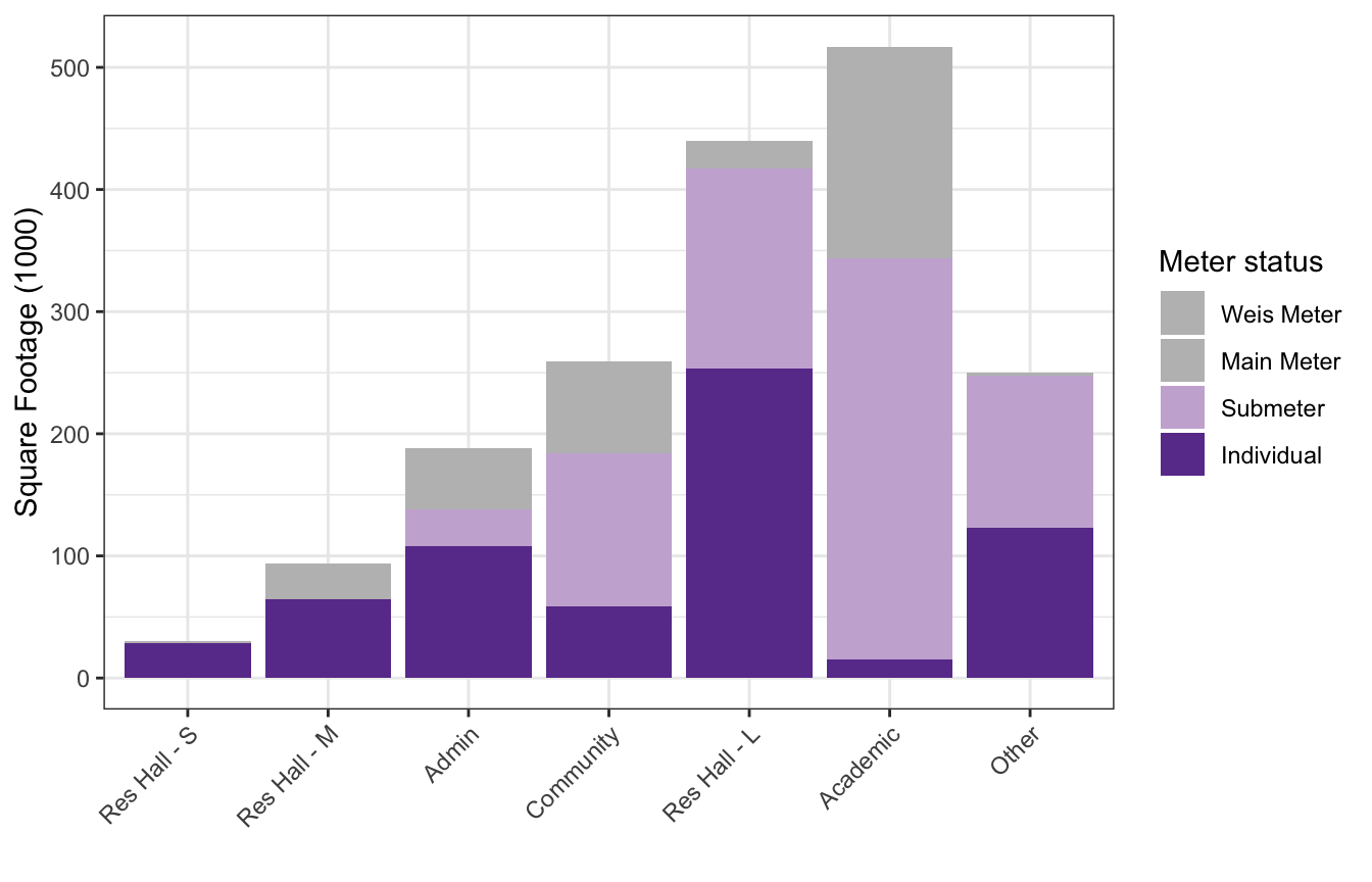
ggplot(buildings_graph,
       aes(x = reorder(type_new, sqft, FUN = "sum"), fill = meter)) +
  geom_bar(position = "stack") +
  scale_fill_manual(values = pal) +
  theme_bw() +
  labs(x = "", y = "Number of Buildings", fill = "Meter status") +
    theme(axis.text.x = element_text(angle = 45, vjust = 1, hjust = 1))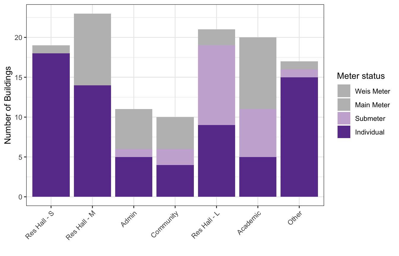
| Version | Author | Date |
|---|---|---|
| e752845 | maggiedouglas | 2026-02-26 |
daily_graph <- daily_full %>%
  mutate(date = as_date(date),
         month = month(date, label = TRUE),
         day = wday(date, label = TRUE),
         type_brief = recode(type,
                       'Res Hall - U' = 'Res Hall',
                       'Res Hall - S' = 'Res Hall',
                       'Res Hall - M' = 'Res Hall',
                       'Res Hall - L' = 'Res Hall')) %>%
  filter(!is.na(month))

ggplot(filter(daily_graph, meter != "Submeter"),
       aes(x = month, y = kwh/10^6, fill = reorder(type_brief, kwh, FUN = sum))) +
  geom_col(position = "stack") +
  scale_fill_brewer(type = "qual", palette = "Paired") +
  theme_bw() +
  labs(x = "", y = "Electricity use (million kWh)", fill = "",
       title = "Electricity use by building type")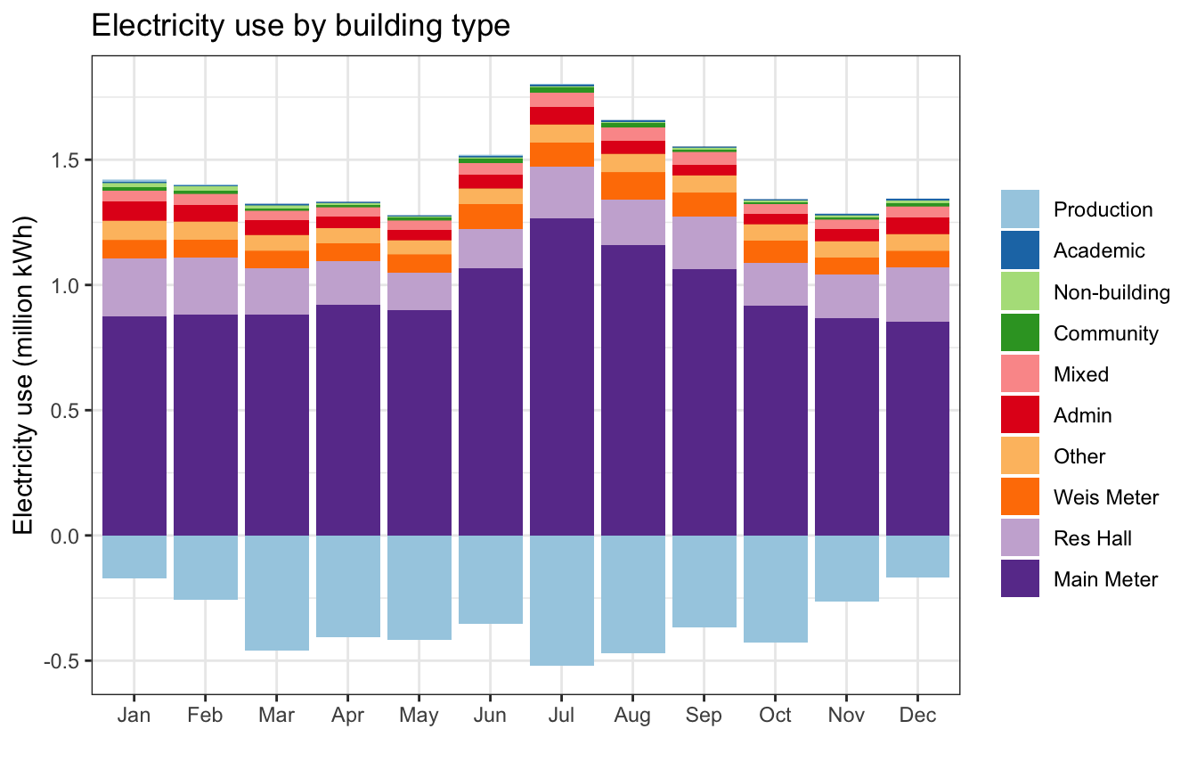
ggplot(filter(daily_graph, meter == "Submeter"),
       aes(x = month, y = kwh/10^6, fill = reorder(type_brief, kwh, FUN = sum))) +
  geom_col(position = "stack") +
  scale_fill_brewer(type = "qual", palette = "Paired") +
  theme_bw() +
  labs(x = "", y = "Electricity use (million kWh)", fill = "",
       title = "Electricity data from the submeters")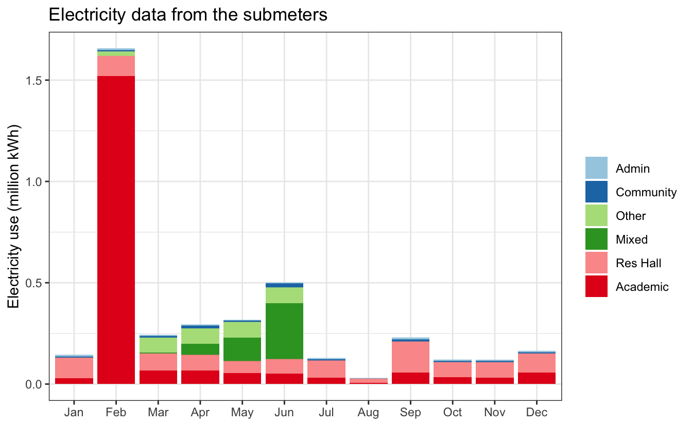
| Version | Author | Date |
|---|---|---|
| e752845 | maggiedouglas | 2026-02-26 |
ggplot(daily_graph, aes(x = month, y = kwh/10^6, fill = reorder(type, kwh, FUN = 'sum'))) +
  geom_col(position = "stack") +
  facet_wrap(. ~ type, scales = "free") +
  theme_bw() +
  labs(x = "", y = "Electricity use (million kWh)", fill = "") +
  theme(axis.text.x = element_text(angle = 90, hjust = 1, vjust = 0.5)) +
  theme(legend.position = "none")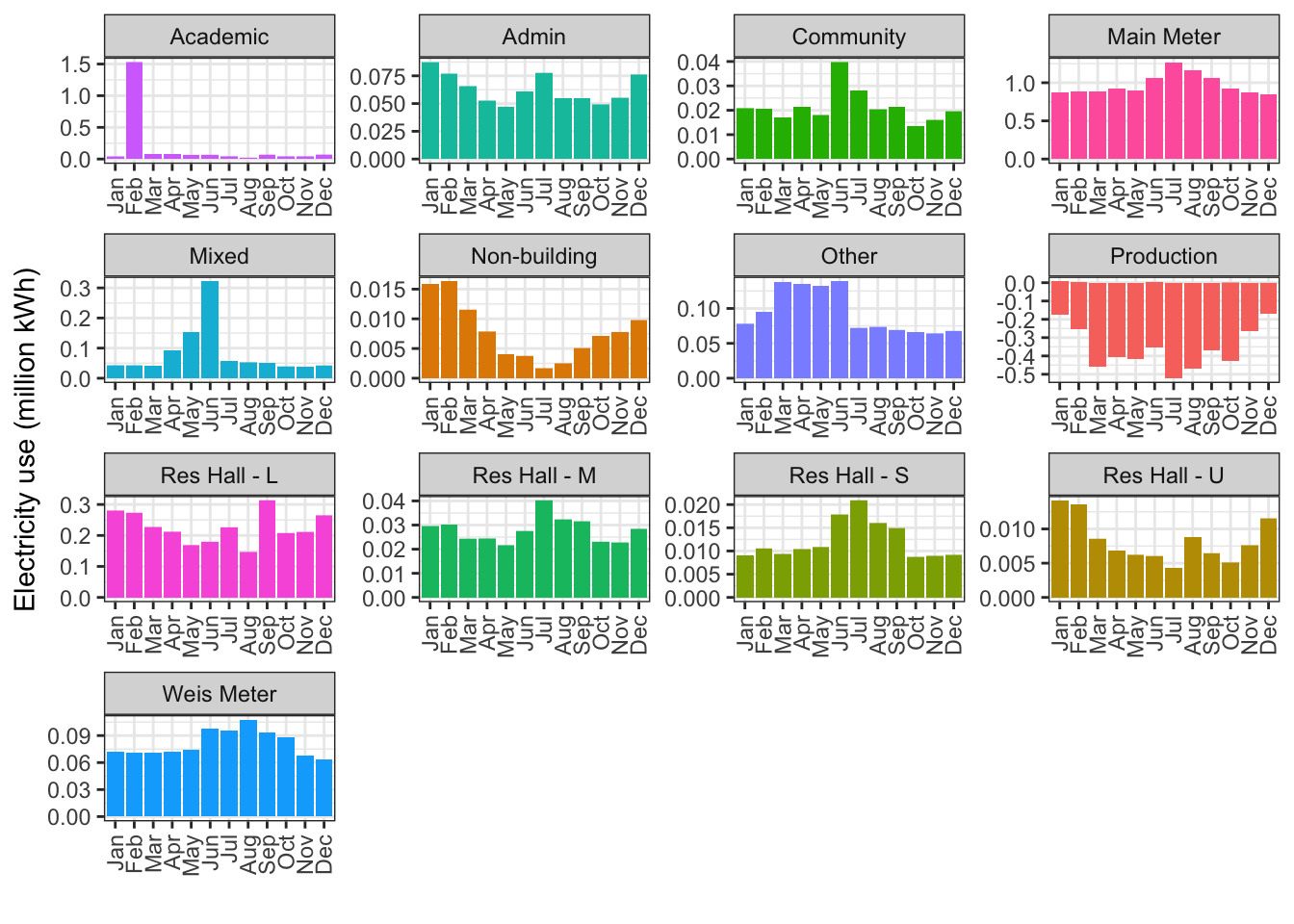
Summary statistics
summary(joined_full) type meter NAME days_perc
Length:104 Length:104 Length:104 Min. : 36.71
Class :character Class :character Class :character 1st Qu.: 95.34
Mode :character Mode :character Mode :character Median :100.00
Mean : 95.72
3rd Qu.:100.00
Max. :100.00
kwh sqft kwh_sqft occupants
Min. :-4274284 Min. : 500 Min. : 0.1624 Min. : 1.000
1st Qu.: 8249 1st Qu.: 1925 1st Qu.: 3.5399 1st Qu.: 4.375
Median : 20783 Median : 5912 Median : 5.1385 Median : 6.000
Mean : 162525 Mean : 30890 Mean : 5.7640 Mean : 28.057
3rd Qu.: 88355 3rd Qu.: 24421 3rd Qu.: 6.5238 3rd Qu.: 33.812
Max. :11648808 Max. :1119435 Max. :23.4772 Max. :159.250
NA's :14 NA's :14 NA's :56
kwh_person dollars ghg_kgCO2
Min. : 797.1 Min. :-347862.9 Min. :-1285808
1st Qu.: 1302.1 1st Qu.: 671.4 1st Qu.: 2482
Median : 1647.3 Median : 1691.4 Median : 6252
Mean : 2706.7 Mean : 13227.1 Mean : 48891
3rd Qu.: 2269.2 3rd Qu.: 7190.8 3rd Qu.: 26579
Max. :19990.2 Max. : 948039.1 Max. : 3504242
NA's :56 ## Stats for campus buildings
stats <- filter(joined_full, meter != "Submeter" & type != "Production")
# million square feet
(sum(joined_agg$sqft, na.rm=T) + sum(joined_individual$sqft, na.rm=T))/10^6[1] 1.946878sum(stats$kwh)/10^6 # million kwh[1] 17.23632sum(stats$dollars)/10^6 # million $[1] 1.402779sum(stats$ghg_kgCO2)/1000 # MT CO2e[1] 5185.1## Stats for solar
solar <- filter(joined_full, type == "Production")
sum(solar$kwh)/10^6 # million kwh[1] -4.274285sum(solar$dollars)/10^6 # million $[1] -0.3478629sum(solar$ghg_kgCO2)/1000 # MT CO2e[1] -1285.808Electricity intensity by type
to_exclude <- filter(joined_full, days_perc < 90)

intensity <- joined_full %>%
  filter(!(type %in% c("Res Hall - U","Production", "Non-building"))
              & !(NAME %in% to_exclude$NAME))

# median and IQR come from EIA (2022) table, annual kWh per square foot for Colleges/Universities
# https://www.eia.gov/consumption/commercial/data/2018/ce/pdf/c22.pdf

ggplot(intensity,
       aes(x = reorder(type, kwh_sqft, FUN = "median"),
                        y = kwh_sqft, fill = type)) +
  annotate("rect", xmin = -Inf, xmax = Inf, ymin = 7.4, ymax = 14.3, color = "lightgray", alpha = 0.3) +
  geom_hline(yintercept = 10.3, linetype = "dashed", color = "white") +
  geom_boxplot() +
  coord_flip() +
  theme_bw() +
  theme(legend.position = "none") +
  labs(x = "", y = "kWh per sqft per year",
       title = "Electricity Intensity by Building Type")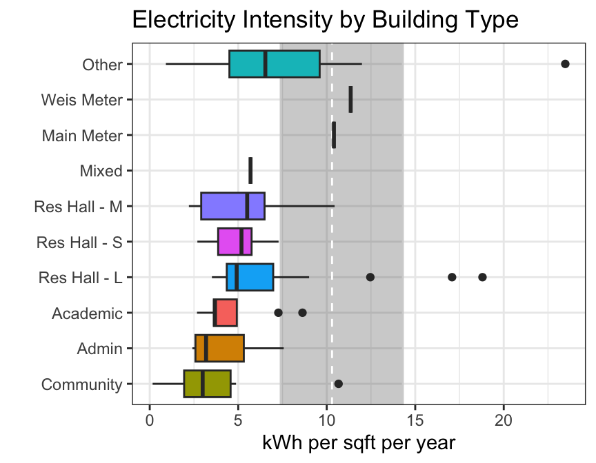
| Version | Author | Date |
|---|---|---|
| e752845 | maggiedouglas | 2026-02-26 |
Export for downstream analyses
joined_exp <- select(joined_full,
                     type, meter, NAME, kwh, sqft, occupants)
daily_exp <- select(daily_full,
                    type, meter, NAME, date, kwh, sqft, ave_temp)

write.csv(daily_exp, "./output/kwh_daily_20260226.csv", row.names = F)
write.csv(joined_exp, "./output/kwh_annual_20260226.csv", row.names = F)
sessionInfo()R version 4.3.2 (2023-10-31)
Platform: x86_64-apple-darwin20 (64-bit)
Running under: macOS Ventura 13.7.8
Matrix products: default
BLAS: /Library/Frameworks/R.framework/Versions/4.3-x86_64/Resources/lib/libRblas.0.dylib
LAPACK: /Library/Frameworks/R.framework/Versions/4.3-x86_64/Resources/lib/libRlapack.dylib; LAPACK version 3.11.0
locale:
[1] en_US.UTF-8/en_US.UTF-8/en_US.UTF-8/C/en_US.UTF-8/en_US.UTF-8
time zone: America/New_York
tzcode source: internal
attached base packages:
[1] stats graphics grDevices utils datasets methods base
other attached packages:
[1] RColorBrewer_1.1-3 scales_1.3.0 DT_0.33 lubridate_1.9.3
[5] forcats_1.0.0 stringr_1.5.1 dplyr_1.1.4 purrr_1.0.2
[9] readr_2.1.5 tidyr_1.3.1 tibble_3.2.1 ggplot2_3.5.1
[13] tidyverse_2.0.0
loaded via a namespace (and not attached):
[1] sass_0.4.8 utf8_1.2.4 generics_0.1.3 stringi_1.8.3
[5] hms_1.1.3 digest_0.6.37 magrittr_2.0.3 timechange_0.3.0
[9] evaluate_0.23 grid_4.3.2 fastmap_1.1.1 rprojroot_2.0.4
[13] workflowr_1.7.1 jsonlite_1.8.8 whisker_0.4.1 promises_1.2.1
[17] fansi_1.0.6 crosstalk_1.2.1 jquerylib_0.1.4 cli_3.6.2
[21] rlang_1.1.3 ellipsis_0.3.2 munsell_0.5.0 withr_3.0.0
[25] cachem_1.0.8 yaml_2.3.8 tools_4.3.2 tzdb_0.4.0
[29] colorspace_2.1-0 httpuv_1.6.13 vctrs_0.6.5 R6_2.5.1
[33] lifecycle_1.0.4 git2r_0.33.0 htmlwidgets_1.6.4 fs_1.6.3
[37] pkgconfig_2.0.3 pillar_1.9.0 bslib_0.6.1 later_1.3.2
[41] gtable_0.3.4 glue_1.7.0 Rcpp_1.1.0 highr_0.10
[45] xfun_0.41 tidyselect_1.2.0 rstudioapi_0.16.0 knitr_1.45
[49] farver_2.1.1 htmltools_0.5.7 labeling_0.4.3 rmarkdown_2.25
[53] compiler_4.3.2