This reproducible R Markdown
analysis was created with workflowr (version
1.7.2). The Checks tab describes the reproducibility checks
that were applied when the results were created. The Past
versions tab lists the development history.
The R Markdown file has unstaged changes. To know which version of
the R Markdown file created these results, you’ll want to first commit
it to the Git repo. If you’re still working on the analysis, you can
ignore this warning. When you’re finished, you can run
wflow_publish to commit the R Markdown file and build the
HTML.
Great job! The global environment was empty. Objects defined in the
global environment can affect the analysis in your R Markdown file in
unknown ways. For reproduciblity it’s best to always run the code in an
empty environment.
The command set.seed(20260127) was run prior to running
the code in the R Markdown file. Setting a seed ensures that any results
that rely on randomness, e.g. subsampling or permutations, are
reproducible.
Great! You are using Git for version control. Tracking code development
and connecting the code version to the results is critical for
reproducibility.
The results in this page were generated with repository version
8386437.
See the Past versions tab to see a history of the changes made
to the R Markdown and HTML files.
Note that you need to be careful to ensure that all relevant files for
the analysis have been committed to Git prior to generating the results
(you can use wflow_publish or
wflow_git_commit). workflowr only checks the R Markdown
file, but you know if there are other scripts or data files that it
depends on. Below is the status of the Git repository when the results
were generated:
Note that any generated files, e.g. HTML, png, CSS, etc., are not
included in this status report because it is ok for generated content to
have uncommitted changes.
These are the previous versions of the repository in which changes were
made to the R Markdown
(analysis/cups_and_skulls_analysis.Rmd) and HTML
(docs/cups_and_skulls_analysis.html) files. If you’ve
configured a remote Git repository (see ?wflow_git_remote),
click on the hyperlinks in the table below to view the files as they
were in that past version.
Add data dictionary worksheet and chamber space analysis
About This Analysis
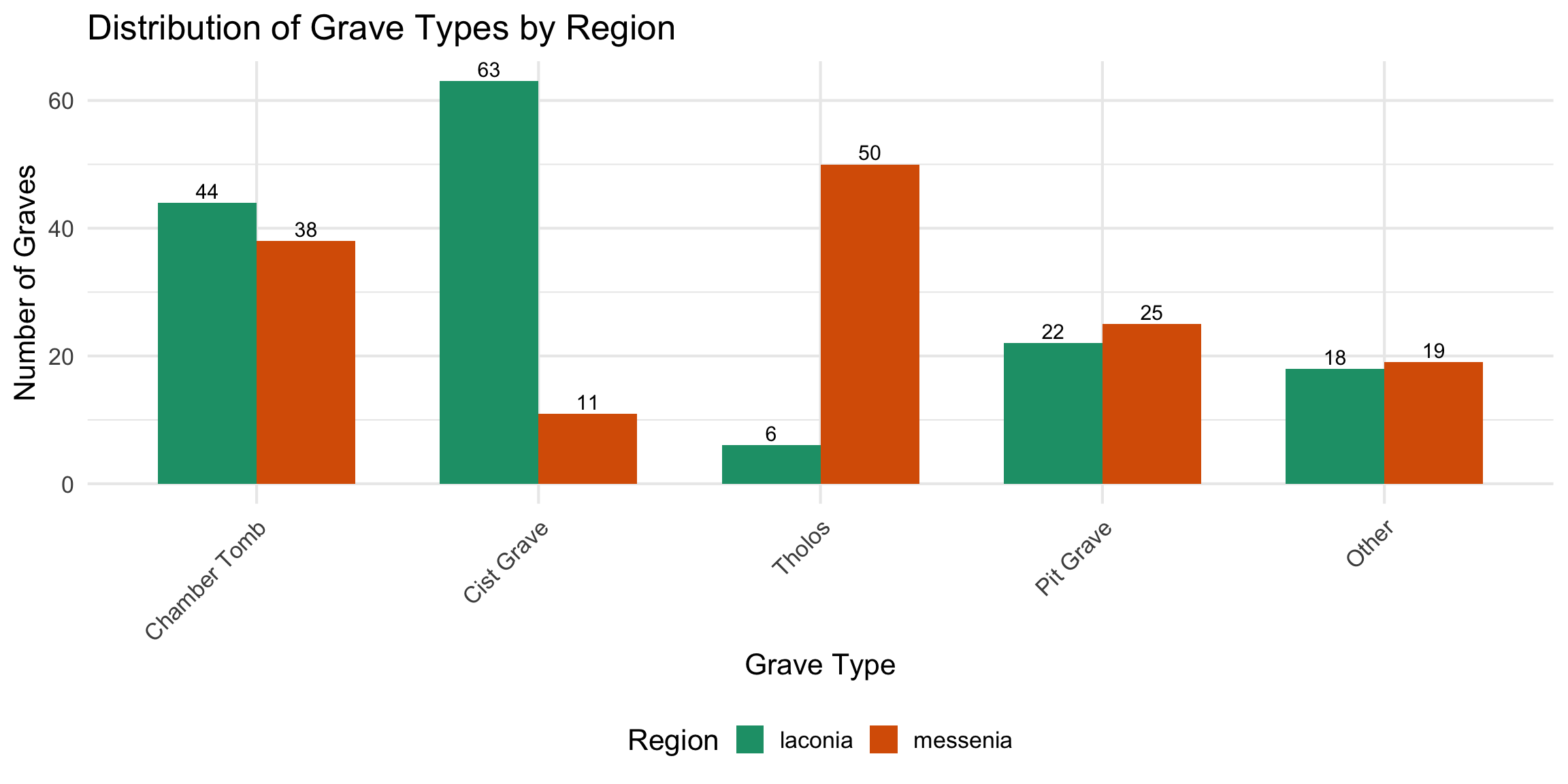
This analysis examines funerary assemblage patterns in Laconia and
Messinia, including:
Distribution comparisons between Laconia and
Messenia
Temporal trends in burial practices across
periods
Hair pin presence and its relationship to secondary
burial, drinking vessels, and tomb size
Regional differences in how graves are used
Relationships between chamber size, drinking
vessels, skeletal remains, and hair pins
Introduction
This analysis examines the relationship between drinking vessels,
human skeletal remains, and hair pins in Laconian and Messinian tholos
and chamber tombs. The data focuses on grave contexts where drinking
vessels and hair pins are recorded alongside information about primary
and secondary burials.
YOU CAN EDIT THIS SECTION: Customize colors for the
analyses. Edit the hex codes below to use your preferred colors.
All plots throughout this analysis will use these colors, so if you
change them here, the change applies everywhere automatically.
Color choices affect: - Regional comparisons
(Laconia vs Messenia) - Visualization clarity and accessibility - How
different variables stand out in plots
# Set your color palette here
colors <- list(
  laconia = "#1B9E77",      # Laconia color (default: teal/green)
  messenia = "#D95F02",     # Messenia color (default: orange)
  drinking_vessel = "#7570B3",  # Drinking vessels (default: purple)
  skulls = "#E7298A",        # Skulls (default: pink)
  pin = "#E6AB02",            # Hair pins (default: gold/amber)
  background = "#FFFFCC"     # Background/neutral (default: light yellow)
)

# These colors will be used throughout all plots
# Change the hex codes to your preferred colors

# Set global ggplot theme with larger text
theme_set(theme_minimal(base_size = 16))
theme_update(
  plot.title = element_text(size = 18, face = "bold"),
  plot.subtitle = element_text(size = 14),
  axis.title = element_text(size = 14),
  axis.text = element_text(size = 12),
  legend.text = element_text(size = 12),
  legend.title = element_text(size = 13),
  strip.text = element_text(size = 13)
)
NOTE: The code below simplifies the complex grave
type names into broader categories. If you want to group grave types
differently, you can edit the case_when() statements in
this chunk. For example, you might want to keep “Pit Grave” and “Cist
Grave” separate, or group them together.
cups_skulls_clean <- cups_skulls %>%
# Clean column names
janitor::clean_names() %>%
# Trim whitespace from character columns
mutate(across(where(is.character), str_trim)) %>%
# Standardize yes/no values in drinking vessel column
mutate(
has_drinking_vessel = case_when(
tolower(drinking_vessel) == "yes" ~ TRUE,
tolower(drinking_vessel) == "no" ~ FALSE,
TRUE ~ NA
),
has_remains = case_when(
tolower(remains) == "yes" ~ TRUE,
tolower(remains) == "no" ~ FALSE,
TRUE ~ NA
),
primary_burial = case_when(
tolower(primary) == "present" ~ TRUE,
tolower(primary) == "absent" ~ FALSE,
TRUE ~ NA
),
secondary_burial = case_when(
tolower(secondary) == "present" ~ TRUE,
tolower(secondary) == "absent" ~ FALSE,
TRUE ~ NA
),
has_pin = case_when(
tolower(hair_pin) == "yes" ~ TRUE,
tolower(hair_pin) == "no" ~ FALSE,
TRUE ~ NA
)
) %>%
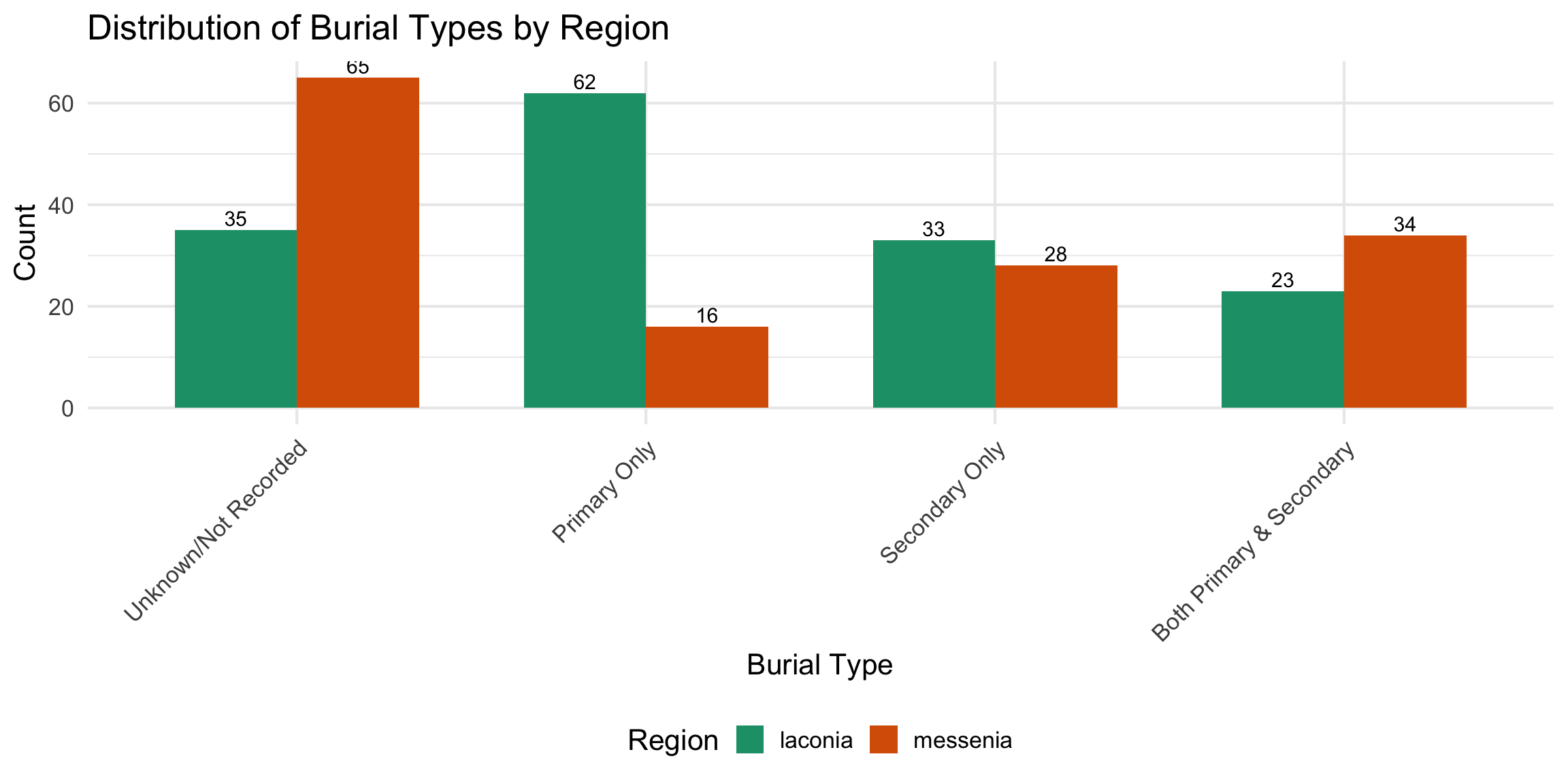
# Create burial category
mutate(
burial_category = case_when(
primary_burial & secondary_burial ~ "Both Primary & Secondary",
primary_burial & !secondary_burial ~ "Primary Only",
!primary_burial & secondary_burial ~ "Secondary Only",
TRUE ~ "Unknown/Not Recorded"
)
) %>%
# Simplify grave type
# ** YOU CAN CUSTOMIZE THIS SECTION **
# If you want different groupings, edit the patterns here
# Current grouping is based on archaeological complexity
mutate(
grave_type_simple = case_when(
str_detect(tolower(type), "tholos") ~ "Tholos",
str_detect(tolower(type), "chamber") ~ "Chamber Tomb",
str_detect(tolower(type), "cist") ~ "Cist Grave",
str_detect(tolower(type), "pit") ~ "Pit Grave",
str_detect(tolower(type), "dromos") ~ "Dromos Only",
TRUE ~ "Other"
)
)
# Show cleaned data structure
glimpse(cups_skulls_clean)
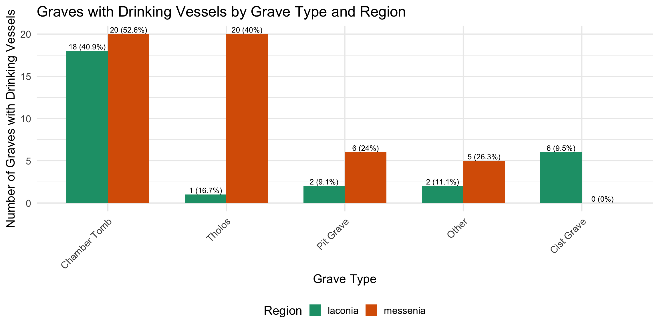
HOW YOUR CHOICES AFFECT THIS: - The groupings in the
“Data Cleaning” section determine what you see here - If you edit
grave_type_simple to create different categories, these
plots will change - Once you complete
tomb_type_dictionary.csv, you can run additional analyses
on tomb complexity
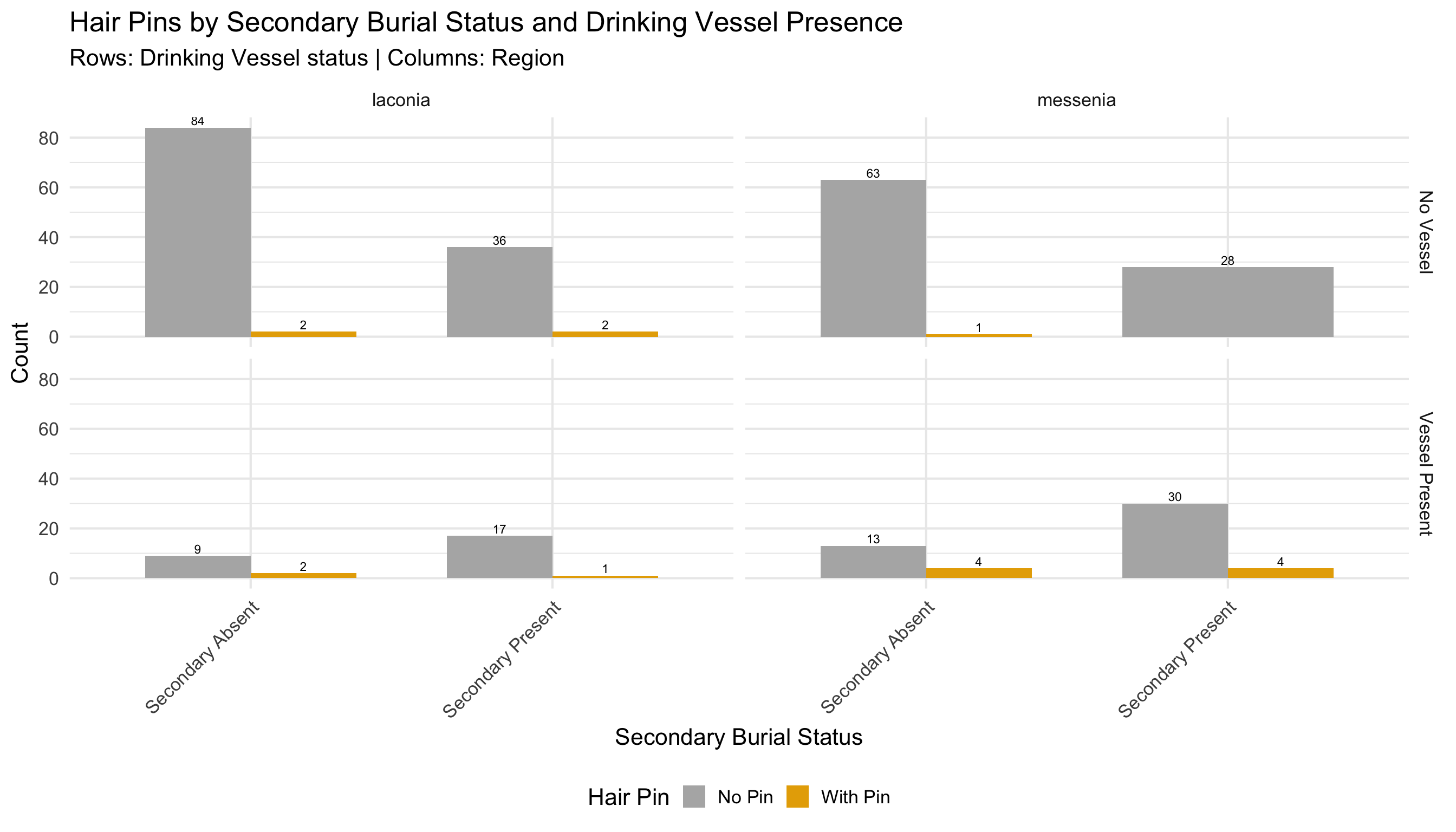
three_way_summary <- cups_skulls_clean %>%
  dplyr::filter(!is.na(has_drinking_vessel) & !is.na(secondary_burial) & !is.na(has_pin)) %>%
  mutate(
    vessel_label = ifelse(has_drinking_vessel, "Vessel Present", "No Vessel"),
    secondary_label = ifelse(secondary_burial, "Secondary Present", "Secondary Absent"),
    pin_label = ifelse(has_pin, "With Pin", "No Pin")
  ) %>%
  count(region, vessel_label, secondary_label, pin_label)

ggplot(three_way_summary, aes(x = secondary_label, y = n, fill = pin_label)) +
  geom_col(position = "dodge", width = 0.7) +
  scale_fill_manual(values = c("With Pin" = colors$pin, "No Pin" = "grey70")) +
  facet_grid(vessel_label ~ region) +
  geom_text(aes(label = n), position = position_dodge(width = 0.7), vjust = -0.3, size = 3) +
  labs(
    title = "Hair Pins by Secondary Burial Status and Drinking Vessel Presence",
    subtitle = "Rows: Drinking Vessel status | Columns: Region",
    x = "Secondary Burial Status",
    y = "Count",
    fill = "Hair Pin"
  ) +
  theme_minimal(base_size = 16) +
  theme(legend.position = "bottom", axis.text.x = element_text(angle = 45, hjust = 1))
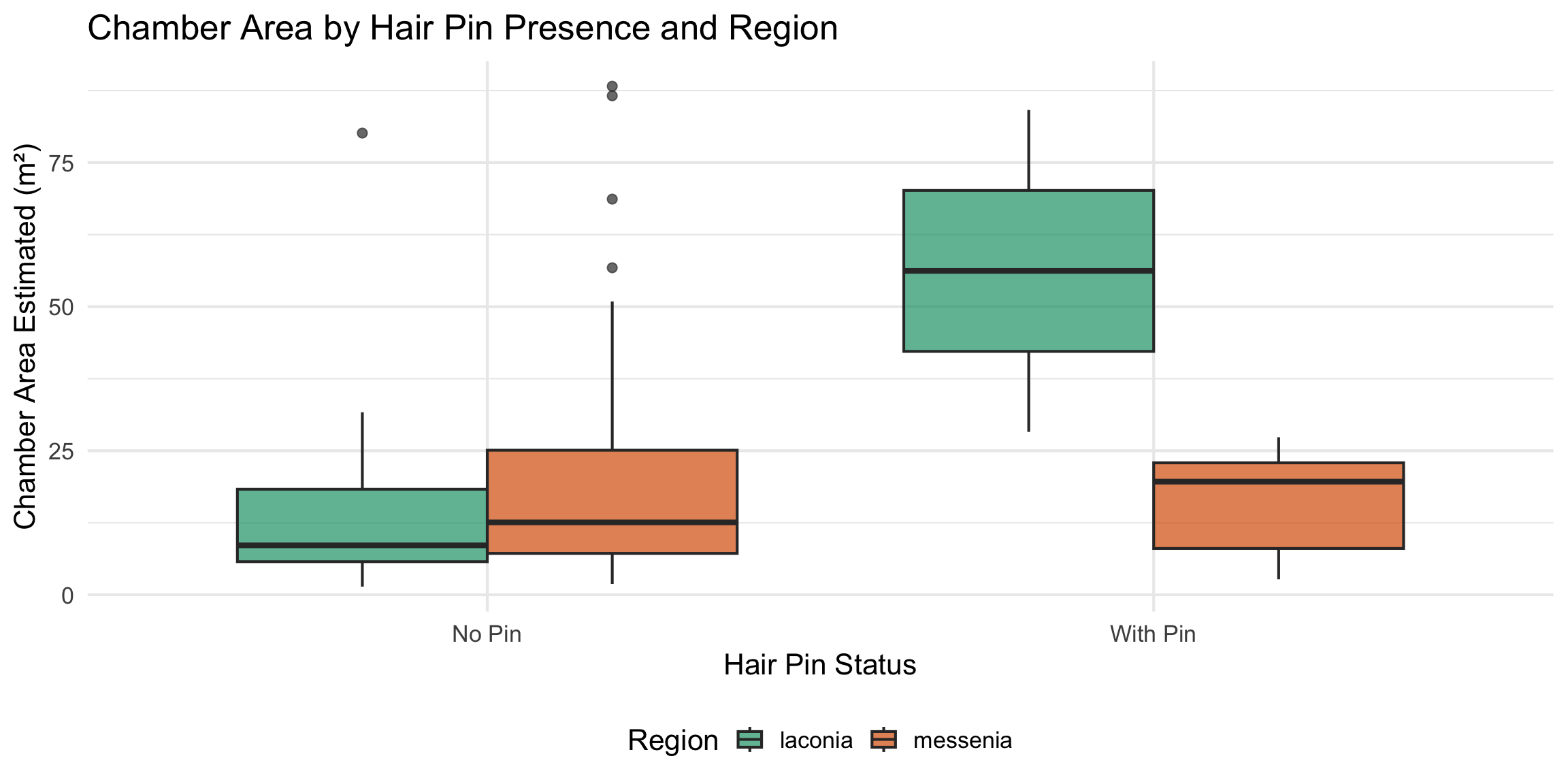
Hair Pins and Chamber Size
Do graves with hair pins tend to be larger?
pins_area_data <- cups_skulls_clean %>%
  dplyr::filter(!is.na(area_of_chamber_estimated) & !is.na(has_pin))

cat("Graves with area AND pin status:", nrow(pins_area_data), "\n")
ggplot(pins_area_data, aes(x = ifelse(has_pin, "With Pin", "No Pin"),
                            y = area_of_chamber_estimated, fill = region)) +
  geom_boxplot(alpha = 0.7, position = "dodge") +
  scale_fill_manual(values = c(laconia = colors$laconia, messenia = colors$messenia)) +
  labs(
    title = "Chamber Area by Hair Pin Presence and Region",
    x = "Hair Pin Status",
    y = "Chamber Area Estimated (m\u00b2)",
    fill = "Region"
  ) +
  theme_minimal(base_size = 16) +
  theme(legend.position = "bottom")
# Wilcoxon test (non-parametric, appropriate for potentially non-normal area data)
for (reg in unique(pins_area_data$region)) {
  region_data <- pins_area_data %>% dplyr::filter(region == reg)
  with_pin <- region_data %>% dplyr::filter(has_pin == TRUE) %>% pull(area_of_chamber_estimated)
  without_pin <- region_data %>% dplyr::filter(has_pin == FALSE) %>% pull(area_of_chamber_estimated)

  cat("\n===", toupper(reg), "===\n")
  cat("With pin: n =", length(with_pin), ", median =", round(median(with_pin), 2), "\n")
  cat("Without pin: n =", length(without_pin), ", median =", round(median(without_pin), 2), "\n")

  if (length(with_pin) >= 2 & length(without_pin) >= 2) {
    test_result <- wilcox.test(with_pin, without_pin)
    cat("Wilcoxon rank-sum test p-value:", round(test_result$p.value, 4), "\n")
  } else {
    cat("Too few observations for statistical test\n")
  }
}
=== LACONIA ===
With pin: n = 2 , median = 56.2
Without pin: n = 29 , median = 8.58
Wilcoxon rank-sum test p-value: 0.0258

=== MESSENIA ===
With pin: n = 5 , median = 19.64
Without pin: n = 63 , median = 12.57
Wilcoxon rank-sum test p-value: 0.8786
# A tibble: 5 × 2
  period_category         graves
  <chr>                    <int>
1 Unrecorded                  90
2 LH III                      88
3 LH I-II                     45
4 Middle Helladic             39
5 Late Helladic (general)     34
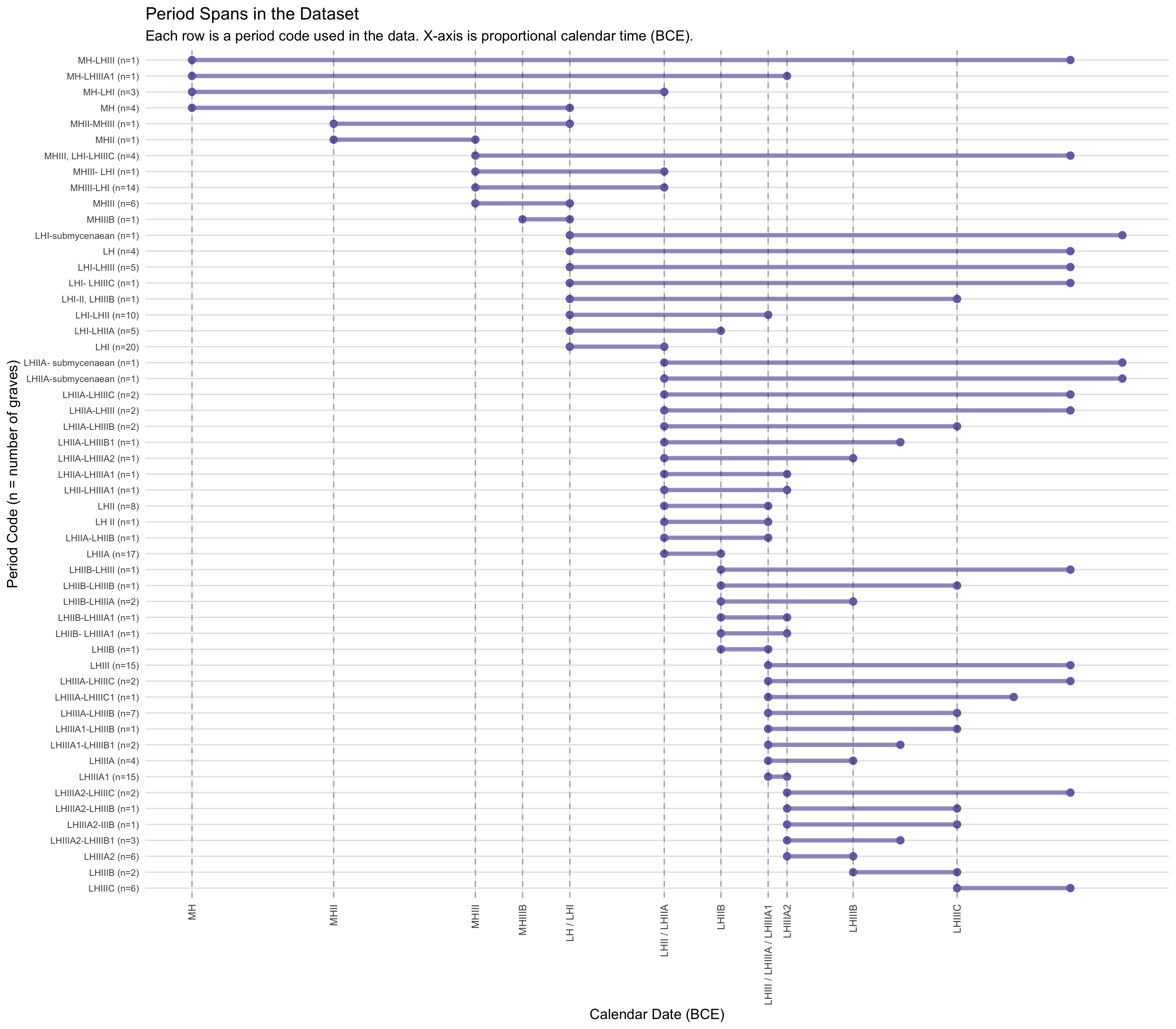
Period Span Analysis
The following chart shows how each period code in the
dataset maps onto the Bronze Age calendar. The x-axis is
proportional to actual calendar years (BCE), so visually wider rows
represent longer date ranges.
Range periods (e.g., “LHIIA–LHIIIB”) appear as
horizontal segments. These indicate that the scholarly record only
places the grave within a span of phases — the grave could date to any
point within that range.
Single-period codes (e.g., “LHIIIA2”) appear as
single points — more precisely dated graves.
The dashed vertical lines mark the start of each
major phase. Tick labels that combine multiple codes (e.g., “LHIII /
LHIIIA / LHIIIA1”) indicate phase boundaries that coincide on the
calendar.
For temporal analyses: Graves with wide-spanning
period codes (long bars) are assigned to the broad phase of their
earliest endpoint. This is the most conservative choice but
means a grave recorded as “MH–LHIIIC” (spanning nearly 1,000 years) is
counted as an MH-phase grave, even though it may represent a much later
context.
# Identify single-component periods and attach calendar years
single_periods <- period_dict %>%
  dplyr::filter(earliest_component == latest_component) %>%
  select(period_code, chronological_order) %>%
  arrange(chronological_order) %>%
  distinct(period_code, .keep_all = TRUE) %>%
  dplyr::filter(period_code != "LH II") %>%
  left_join(component_cal %>% select(component, cal_start_bce),
            by = c("period_code" = "component"))

# Get all period codes in the data with their calendar year spans
period_spans <- cups_skulls_clean %>%
  dplyr::filter(!is.na(period_start_cal) & !is.na(period_end_cal)) %>%
  distinct(period, period_start_cal, period_end_cal) %>%
  mutate(
    is_range = period_start_cal != period_end_cal,
    span_width = period_start_cal - period_end_cal  # BCE: larger start = earlier
  ) %>%
  arrange(desc(period_start_cal), period_end_cal)

# Count graves per period code
period_counts <- cups_skulls_clean %>%
  dplyr::filter(!is.na(period_start_cal)) %>%
  count(period, name = "n_graves")

period_spans <- period_spans %>%
  left_join(period_counts, by = "period") %>%
  mutate(period_label = paste0(period, " (n=", n_graves, ")")) %>%
  mutate(period_label = factor(period_label,
    levels = rev(mutate(arrange(., desc(period_start_cal), period_end_cal),
                        period_label = paste0(period, " (n=", n_graves, ")"))$period_label)))

# Collapse period codes that share the same calendar position into one label
# (e.g. LH and LHI both start at 1600 BCE — combine as "LH / LHI")
single_periods_unique <- dplyr::filter(single_periods, !is.na(cal_start_bce)) %>%
  group_by(cal_start_bce) %>%
  summarise(period_code = paste(period_code, collapse = " / "), .groups = "drop")

ggplot(period_spans) +
  geom_segment(
    data = dplyr::filter(period_spans, is_range),
    aes(x = period_start_cal, xend = period_end_cal,
        y = period_label, yend = period_label),
    linewidth = 2, color = colors$drinking_vessel, alpha = 0.7
  ) +
  geom_point(
    aes(x = period_start_cal, y = period_label),
    size = 3, color = colors$drinking_vessel
  ) +
  geom_point(
    data = dplyr::filter(period_spans, is_range),
    aes(x = period_end_cal, y = period_label),
    size = 3, color = colors$drinking_vessel
  ) +
  geom_vline(
    data = single_periods_unique,
    aes(xintercept = cal_start_bce),
    linetype = "dashed", alpha = 0.3
  ) +
  scale_x_reverse(
    breaks = single_periods_unique$cal_start_bce,
    labels = single_periods_unique$period_code
  ) +
  labs(
    title = "Period Spans in the Dataset",
    subtitle = "Each row is a period code used in the data. X-axis is proportional calendar time (BCE).",
    x = "Calendar Date (BCE)",
    y = "Period Code (n = number of graves)"
  ) +
  theme_minimal(base_size = 14) +
  theme(
    axis.text.x = element_text(angle = 90, hjust = 1, vjust = 0.5, size = 10),
    axis.text.y = element_text(size = 9),
    panel.grid.major.y = element_line(color = "grey90"),
    panel.grid.minor = element_blank()
  )
cat("=== Individual chronological components (in order) ===\n\n")
=== Individual chronological components (in order) ===
for (i in 1:nrow(single_periods)) {
  cat(sprintf("  %2d. %s\n", i, single_periods$period_code[i]))
}
cat("Total period codes in data:", nrow(period_spans), "\n")
Total period codes in data: 53
cat("\n=== Range periods spanning 3+ components ===\n")
=== Range periods spanning 3+ components ===
wide_spans <- period_spans %>%
  dplyr::filter(span_width > 10) %>%
  arrange(desc(span_width))
if (nrow(wide_spans) > 0) {
  for (i in 1:nrow(wide_spans)) {
    cat(sprintf("  %s: spans from order %g to %g (width = %g, n = %d graves)\n",
        wide_spans$period[i], wide_spans$period_start_order[i],
        wide_spans$period_end_order[i], wide_spans$span_width[i],
        wide_spans$n_graves[i]))
  }
}
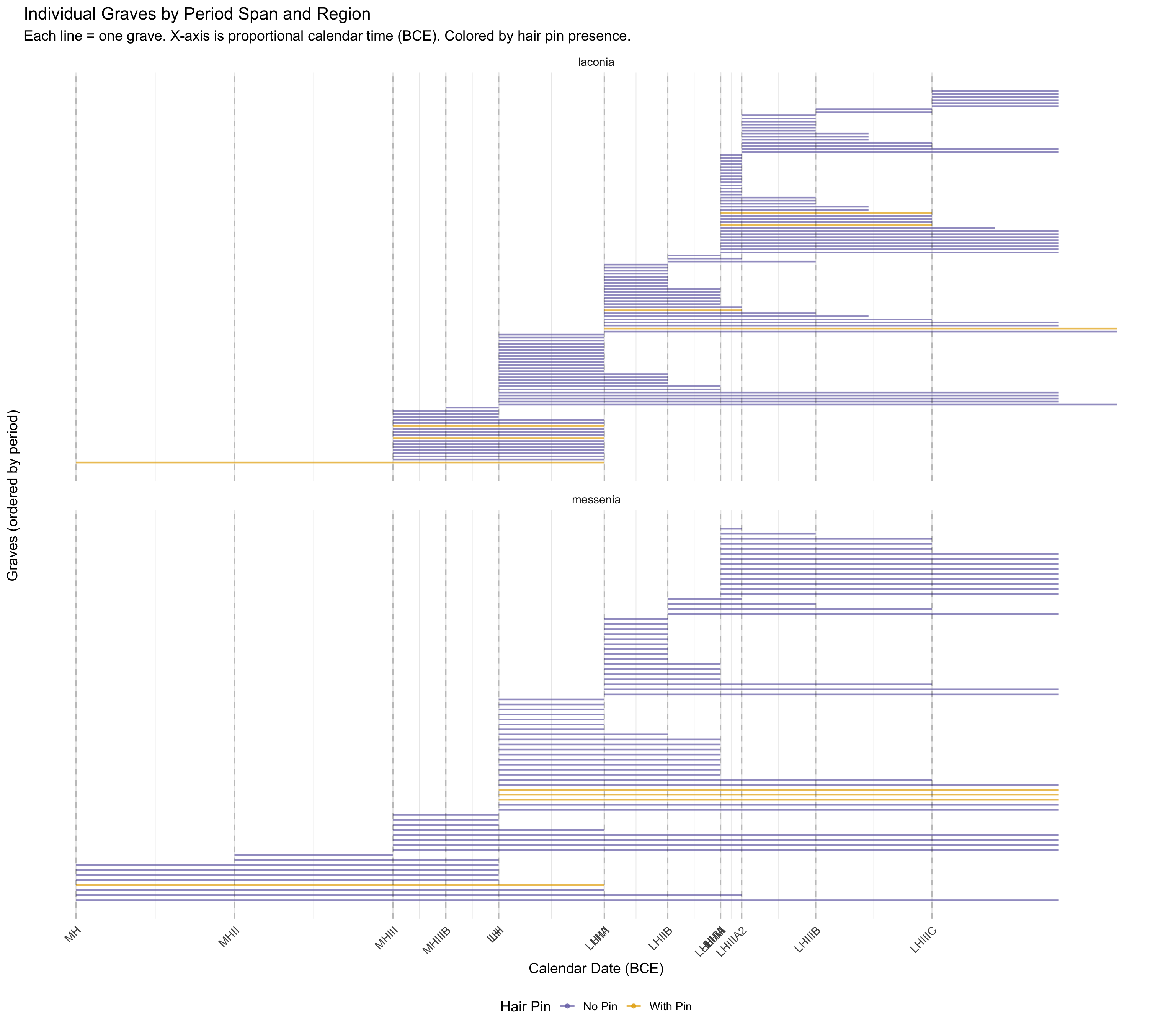
Individual Graves by Period and Region
Each line represents a single grave, spanning its period range.
Graves are colored by whether hair pins were found. This shows how
graves cluster across time and whether pin-bearing graves concentrate in
particular periods.
# Prepare individual grave data with calendar year spans
graves_time <- cups_skulls_clean %>%
  dplyr::filter(!is.na(period_start_cal) & !is.na(period_end_cal) & !is.na(has_pin)) %>%
  mutate(pin_label = ifelse(has_pin, "With Pin", "No Pin")) %>%
  # Order graves: earlier start first (higher BCE = earlier), then narrower range
  arrange(region, desc(period_start_cal), period_end_cal) %>%
  group_by(region) %>%
  mutate(grave_rank = row_number()) %>%
  ungroup()

# Use single_periods with cal years (already built in period-span-chart chunk)
sp_cal <- dplyr::filter(single_periods, !is.na(cal_start_bce))

ggplot(graves_time) +
  geom_segment(
    aes(x = period_start_cal, xend = period_end_cal,
        y = grave_rank, yend = grave_rank,
        color = pin_label),
    linewidth = 0.8, alpha = 0.7
  ) +
  geom_point(
    data = dplyr::filter(graves_time, period_start_cal == period_end_cal),
    aes(x = period_start_cal, y = grave_rank, color = pin_label),
    size = 1.5, alpha = 0.7
  ) +
  scale_color_manual(values = c("With Pin" = colors$pin, "No Pin" = colors$drinking_vessel)) +
  geom_vline(
    data = sp_cal,
    aes(xintercept = cal_start_bce),
    linetype = "dashed", alpha = 0.2
  ) +
  scale_x_reverse(
    breaks = sp_cal$cal_start_bce,
    labels = sp_cal$period_code
  ) +
  facet_wrap(~region, ncol = 1, scales = "free_y") +
  labs(
    title = "Individual Graves by Period Span and Region",
    subtitle = "Each line = one grave. X-axis is proportional calendar time (BCE). Colored by hair pin presence.",
    x = "Calendar Date (BCE)",
    y = "Graves (ordered by period)",
    color = "Hair Pin"
  ) +
  theme_minimal(base_size = 14) +
  theme(
    legend.position = "bottom",
    axis.text.x = element_text(angle = 45, hjust = 1, size = 11),
    axis.text.y = element_blank(),
    axis.ticks.y = element_blank(),
    panel.grid.major.y = element_blank(),
    panel.grid.minor.y = element_blank()
  )
Temporal Analyses
The purpose of this section is to examine whether funerary practices
— burial type, presence of drinking vessels, hair pins, and tomb size —
changed over the course of the Bronze Age and whether those changes
differed between Laconia and Messenia.
How Graves Are Assigned to Phases
Graves in this dataset are often given date ranges
rather than a single period (e.g., a grave might be recorded as
“LHIIA–LHIIIB,” meaning it could date anywhere within that span). For
the temporal plots below, each grave is assigned to the 7-phase
broad phase scheme (MH → SM) based on its
earliest period component. A grave dated LHIIA–LHIIIB,
for instance, is counted in “LH II” — its earliest possible phase.
What this means for interpretation: A grave assigned
to an early phase may actually be a later burial; the assignment is
conservative (if anything, it understates change over time). Graves
spanning many centuries are the most ambiguous, and their placement in
the earliest phase is a simplification.
Excluded graves: Graves whose period code could not
be matched to any known component (i.e., those with unusual or
incomplete period designations) receive NA for
broad_phase and are excluded from all temporal
plots. The table below shows how many graves fall into each
phase, including the NA count. Additionally, graves recorded only as the
generic undifferentiated “LH” code are assigned to “LH I” (the earliest
LH sub-phase), which may slightly inflate that category.
Two display options are shown for each plot:
Option A — Ordered categorical x-axis (7 broad
phases as labels, equal spacing)
Option B — Proportional calendar x-axis (BCE years,
bar widths scaled to actual phase duration)
     MH    LH I   LH II LH IIIA LH IIIB LH IIIC      SM    <NA>
     37      47      46      60       2       6       0      98
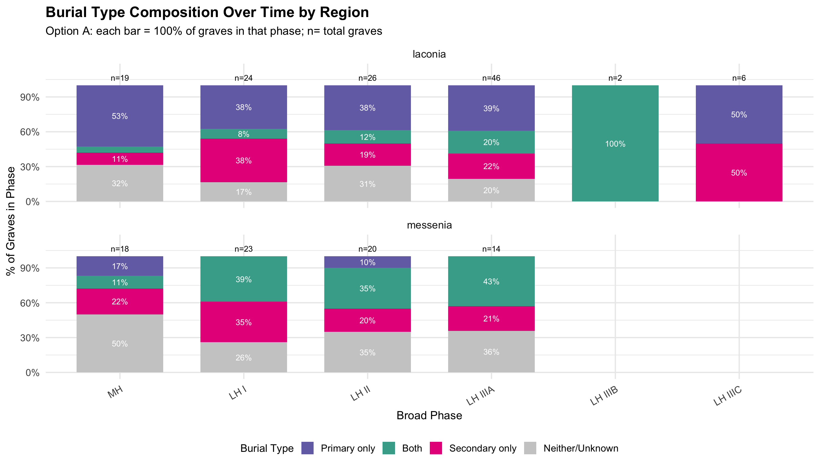
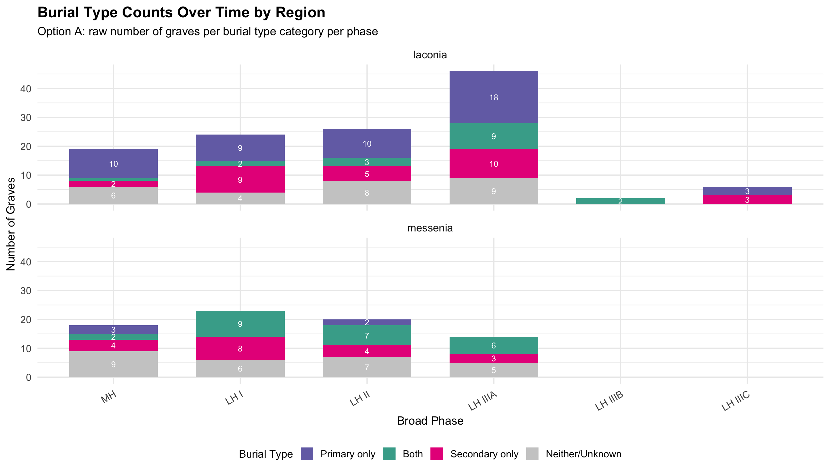
Burial Type Composition Over Time
These charts show whether the mix of primary and secondary
burials changed over time within each region. Primary burial
refers to an intact, articulated interment of a body; secondary burial
refers to the later re-deposition of skeletal remains (typically
disarticulated bones moved to make room for new burials). A single grave
can contain both.
Each grave is classified into one of four mutually
exclusive categories: - Primary only —
evidence for primary burial, no secondary - Both —
evidence for both primary and secondary burials - Secondary
only — evidence for secondary burial only -
Neither/Unknown — no burial type recorded
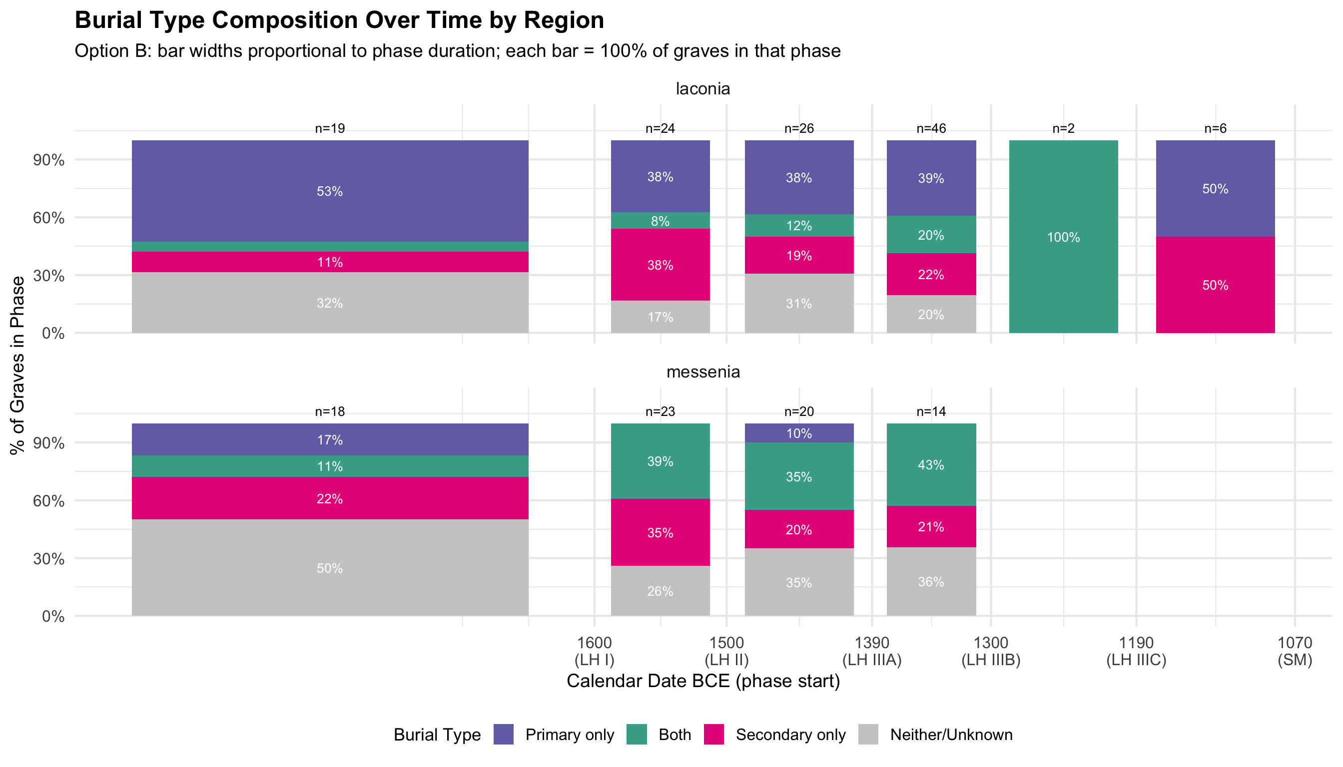
Bars show 100% of graves dated to that phase in that
region; n= total graves in the phase. The “Neither/Unknown”
segment is important: it reflects gaps in the recording — graves where
burial type was not noted, not necessarily graves without burials. A
large “Neither/Unknown” segment in a phase indicates the available data
for that period is limited.
Option A: Broad Phase Categories — Proportions
burial_cat_data <- cups_skulls_clean %>%
  dplyr::filter(!is.na(broad_phase)) %>%
  mutate(burial_cat = case_when(
    primary_burial == TRUE & secondary_burial == TRUE ~ "Both",
    primary_burial == TRUE                            ~ "Primary only",
    secondary_burial == TRUE                          ~ "Secondary only",
    TRUE                                              ~ "Neither/Unknown"
  ),
  burial_cat = factor(burial_cat,
    levels = c("Primary only", "Both", "Secondary only", "Neither/Unknown"))) %>%
  group_by(region, broad_phase, burial_cat) %>%
  summarise(n = n(), .groups = "drop") %>%
  group_by(region, broad_phase) %>%
  mutate(total = sum(n), pct = n / total * 100) %>%
  ungroup()

phase_totals_burial <- burial_cat_data %>%
  distinct(region, broad_phase, total)

ggplot(burial_cat_data, aes(x = broad_phase, y = pct, fill = burial_cat)) +
  geom_col(position = "stack", width = 0.7) +
  geom_text(aes(label = ifelse(pct >= 8, paste0(round(pct), "%"), "")),
            position = position_stack(vjust = 0.5), size = 3.5, color = "white") +
  geom_text(data = phase_totals_burial,
            aes(x = broad_phase, y = 104, label = paste0("n=", total)),
            inherit.aes = FALSE, vjust = 0, size = 3.5) +
  scale_fill_manual(values = c(
    "Primary only"    = colors$drinking_vessel,
    "Both"            = "#44AA99",
    "Secondary only"  = colors$skulls,
    "Neither/Unknown" = "grey80"
  )) +
  scale_y_continuous(limits = c(0, 113), labels = function(x) paste0(x, "%")) +
  facet_wrap(~region, ncol = 1) +
  labs(
    title = "Burial Type Composition Over Time by Region",
    subtitle = "Option A: each bar = 100% of graves in that phase; n= total graves",
    x = "Broad Phase", y = "% of Graves in Phase", fill = "Burial Type"
  ) +
  theme(legend.position = "bottom", axis.text.x = element_text(angle = 30, hjust = 1))
Option A: Raw Counts
ggplot(burial_cat_data, aes(x = broad_phase, y = n, fill = burial_cat)) +
  geom_col(position = "stack", width = 0.7) +
  geom_text(aes(label = ifelse(n >= 2, n, "")),
            position = position_stack(vjust = 0.5), size = 3.5, color = "white") +
  scale_fill_manual(values = c(
    "Primary only"    = colors$drinking_vessel,
    "Both"            = "#44AA99",
    "Secondary only"  = colors$skulls,
    "Neither/Unknown" = "grey80"
  )) +
  facet_wrap(~region, ncol = 1) +
  labs(
    title = "Burial Type Counts Over Time by Region",
    subtitle = "Option A: raw number of graves per burial type category per phase",
    x = "Broad Phase", y = "Number of Graves", fill = "Burial Type"
  ) +
  theme(legend.position = "bottom", axis.text.x = element_text(angle = 30, hjust = 1))
Option B: Proportional Calendar Time (BCE) — Proportions
burial_cat_b <- burial_cat_data %>%
  left_join(phase_cal, by = "broad_phase") %>%
  mutate(bar_width = phase_duration * 0.75)

phase_totals_burial_b <- burial_cat_b %>%
  distinct(region, broad_phase, total, phase_mid_bce)

ggplot(burial_cat_b, aes(x = phase_mid_bce, y = pct, fill = burial_cat, width = bar_width)) +
  geom_col(position = "stack") +
  geom_text(aes(label = ifelse(pct >= 8, paste0(round(pct), "%"), "")),
            position = position_stack(vjust = 0.5), size = 3.5, color = "white") +
  geom_text(data = phase_totals_burial_b,
            aes(x = phase_mid_bce, y = 104, label = paste0("n=", total)),
            inherit.aes = FALSE, vjust = 0, size = 3.5) +
  scale_fill_manual(values = c(
    "Primary only"    = colors$drinking_vessel,
    "Both"            = "#44AA99",
    "Secondary only"  = colors$skulls,
    "Neither/Unknown" = "grey80"
  )) +
  scale_y_continuous(limits = c(0, 113), labels = function(x) paste0(x, "%")) +
  scale_x_reverse(
    breaks = phase_cal$phase_start_bce,
    labels = paste0(phase_cal$phase_start_bce, "\n(", phase_cal$broad_phase, ")")
  ) +
  facet_wrap(~region, ncol = 1) +
  labs(
    title = "Burial Type Composition Over Time by Region",
    subtitle = "Option B: bar widths proportional to phase duration; each bar = 100% of graves in that phase",
    x = "Calendar Date BCE (phase start)", y = "% of Graves in Phase", fill = "Burial Type"
  ) +
  theme(legend.position = "bottom")
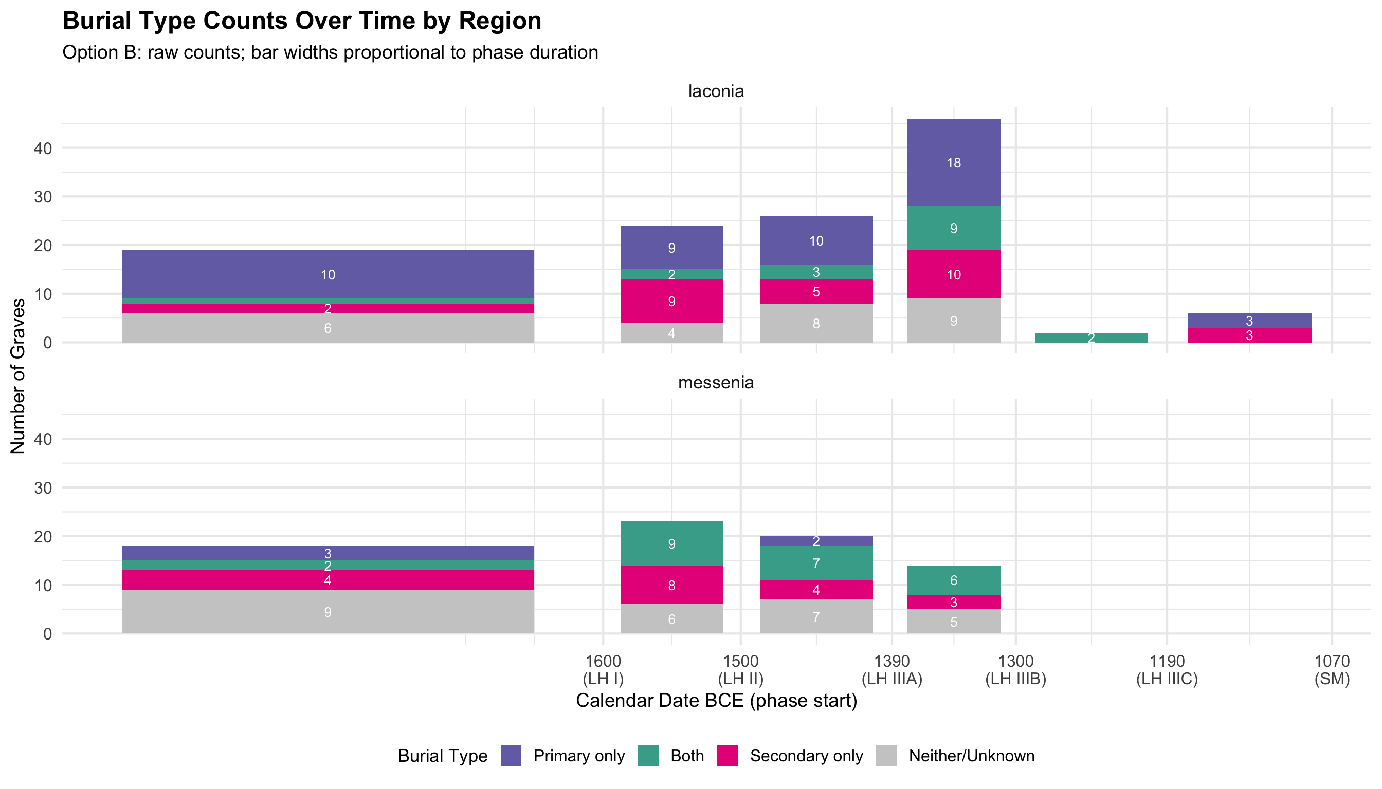
Option B: Raw Counts
ggplot(burial_cat_b, aes(x = phase_mid_bce, y = n, fill = burial_cat, width = bar_width)) +
  geom_col(position = "stack") +
  geom_text(aes(label = ifelse(n >= 2, n, "")),
            position = position_stack(vjust = 0.5), size = 3.5, color = "white") +
  scale_fill_manual(values = c(
    "Primary only"    = colors$drinking_vessel,
    "Both"            = "#44AA99",
    "Secondary only"  = colors$skulls,
    "Neither/Unknown" = "grey80"
  )) +
  scale_x_reverse(
    breaks = phase_cal$phase_start_bce,
    labels = paste0(phase_cal$phase_start_bce, "\n(", phase_cal$broad_phase, ")")
  ) +
  facet_wrap(~region, ncol = 1) +
  labs(
    title = "Burial Type Counts Over Time by Region",
    subtitle = "Option B: raw counts; bar widths proportional to phase duration",
    x = "Calendar Date BCE (phase start)", y = "Number of Graves", fill = "Burial Type"
  ) +
  theme(legend.position = "bottom")
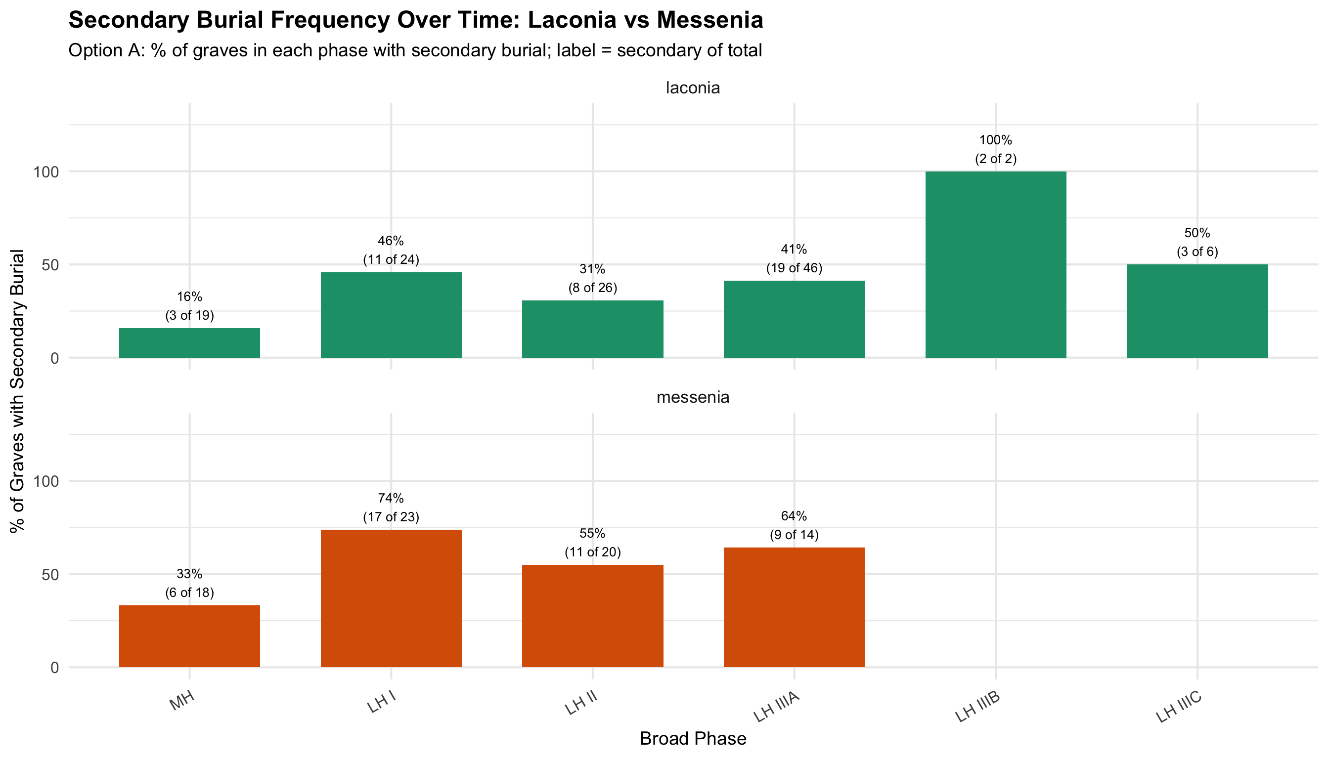
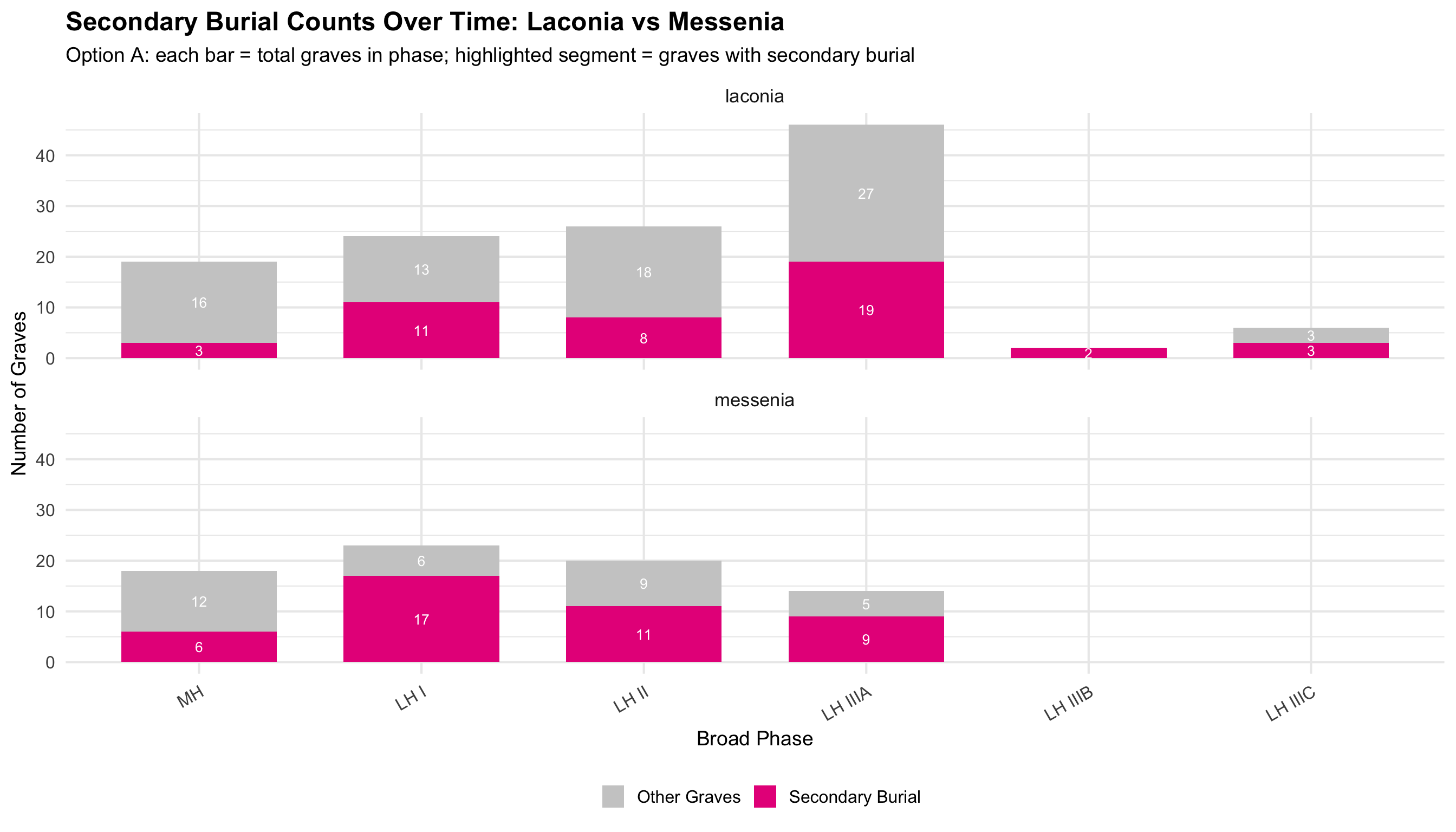
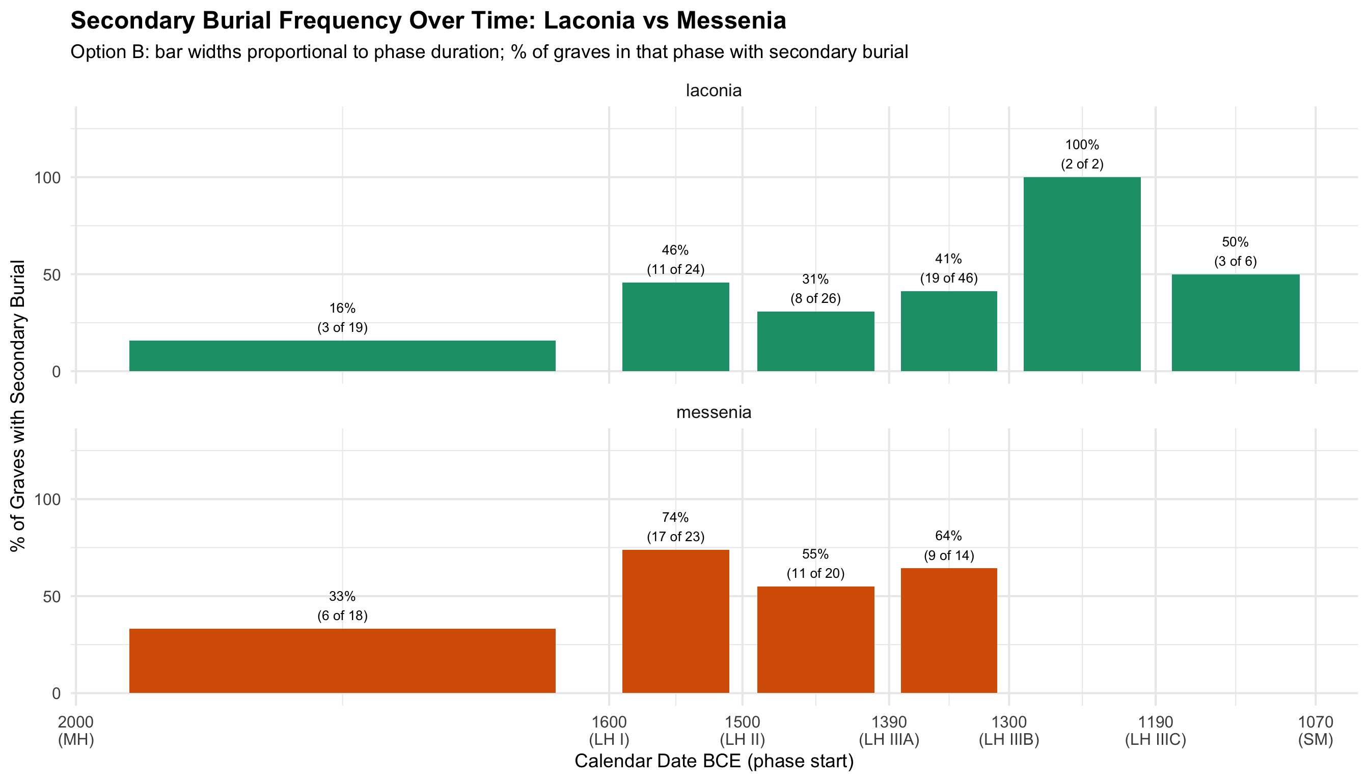
Regional Comparison: Secondary Burial Over Time
These plots isolate the secondary burial rate — the
proportion of graves in each phase with evidence for secondary burial —
and compare Laconia and Messenia directly. The two regions are stacked
top-to-bottom to make the x-axis comparable at a glance.
What to look for: Do the two regions track together
(suggesting pan-regional practice) or diverge (suggesting regional
differences in how and when secondary burial became common)? Phases with
very small n (shown in the labels) should be interpreted cautiously — a
single grave shifts the percentage dramatically.
Labels show “X% (N secondary of M total graves in that phase).”
Option A: Broad Phase Categories — Proportions
secondary_phase <- cups_skulls_clean %>%
  dplyr::filter(!is.na(broad_phase) & !is.na(secondary_burial)) %>%
  group_by(region, broad_phase) %>%
  summarise(
    n_graves    = n(),
    n_secondary = sum(secondary_burial == TRUE),
    pct_secondary = round(n_secondary / n_graves * 100, 1),
    .groups = "drop"
  )

ggplot(secondary_phase, aes(x = broad_phase, y = pct_secondary, fill = region)) +
  geom_col(width = 0.7) +
  geom_text(aes(label = paste0(round(pct_secondary), "%\n(", n_secondary, " of ", n_graves, ")")),
            vjust = -0.3, size = 3.5) +
  scale_fill_manual(values = c(laconia = colors$laconia, messenia = colors$messenia)) +
  scale_y_continuous(limits = c(0, 130)) +
  facet_wrap(~region, ncol = 1) +
  labs(
    title = "Secondary Burial Frequency Over Time: Laconia vs Messenia",
    subtitle = "Option A: % of graves in each phase with secondary burial; label = secondary of total",
    x = "Broad Phase", y = "% of Graves with Secondary Burial", fill = "Region"
  ) +
  theme(legend.position = "none", axis.text.x = element_text(angle = 30, hjust = 1))
Option A: Raw Counts
secondary_raw_stack <- secondary_phase %>%
  mutate(n_other = n_graves - n_secondary) %>%
  pivot_longer(cols = c(n_secondary, n_other),
               names_to = "burial_type", values_to = "count") %>%
  mutate(burial_type = ifelse(burial_type == "n_secondary", "Secondary Burial", "Other Graves"))

ggplot(secondary_raw_stack, aes(x = broad_phase, y = count, fill = burial_type)) +
  geom_col(position = "stack", width = 0.7) +
  geom_text(aes(label = ifelse(count > 0, count, "")),
            position = position_stack(vjust = 0.5), size = 3.5, color = "white") +
  scale_fill_manual(values = c("Secondary Burial" = colors$skulls, "Other Graves" = "grey80")) +
  facet_wrap(~region, ncol = 1) +
  labs(
    title = "Secondary Burial Counts Over Time: Laconia vs Messenia",
    subtitle = "Option A: each bar = total graves in phase; highlighted segment = graves with secondary burial",
    x = "Broad Phase", y = "Number of Graves", fill = ""
  ) +
  theme(legend.position = "bottom", axis.text.x = element_text(angle = 30, hjust = 1))
Option B: Proportional Calendar Time (BCE) — Proportions
secondary_phase_b <- secondary_phase %>%
  left_join(phase_cal, by = "broad_phase") %>%
  mutate(bar_width = phase_duration * 0.8)

ggplot(secondary_phase_b,
       aes(x = phase_mid_bce, y = pct_secondary, fill = region, width = bar_width)) +
  geom_col(position = "identity") +
  geom_text(aes(label = paste0(round(pct_secondary), "%\n(", n_secondary, " of ", n_graves, ")")),
            vjust = -0.3, size = 3.5) +
  scale_fill_manual(values = c(laconia = colors$laconia, messenia = colors$messenia)) +
  scale_y_continuous(limits = c(0, 130)) +
  scale_x_reverse(
    breaks = phase_cal$phase_start_bce,
    labels = paste0(phase_cal$phase_start_bce, "\n(", phase_cal$broad_phase, ")")
  ) +
  facet_wrap(~region, ncol = 1) +
  labs(
    title = "Secondary Burial Frequency Over Time: Laconia vs Messenia",
    subtitle = "Option B: bar widths proportional to phase duration; % of graves in that phase with secondary burial",
    x = "Calendar Date BCE (phase start)", y = "% of Graves with Secondary Burial", fill = "Region"
  ) +
  theme(legend.position = "none")
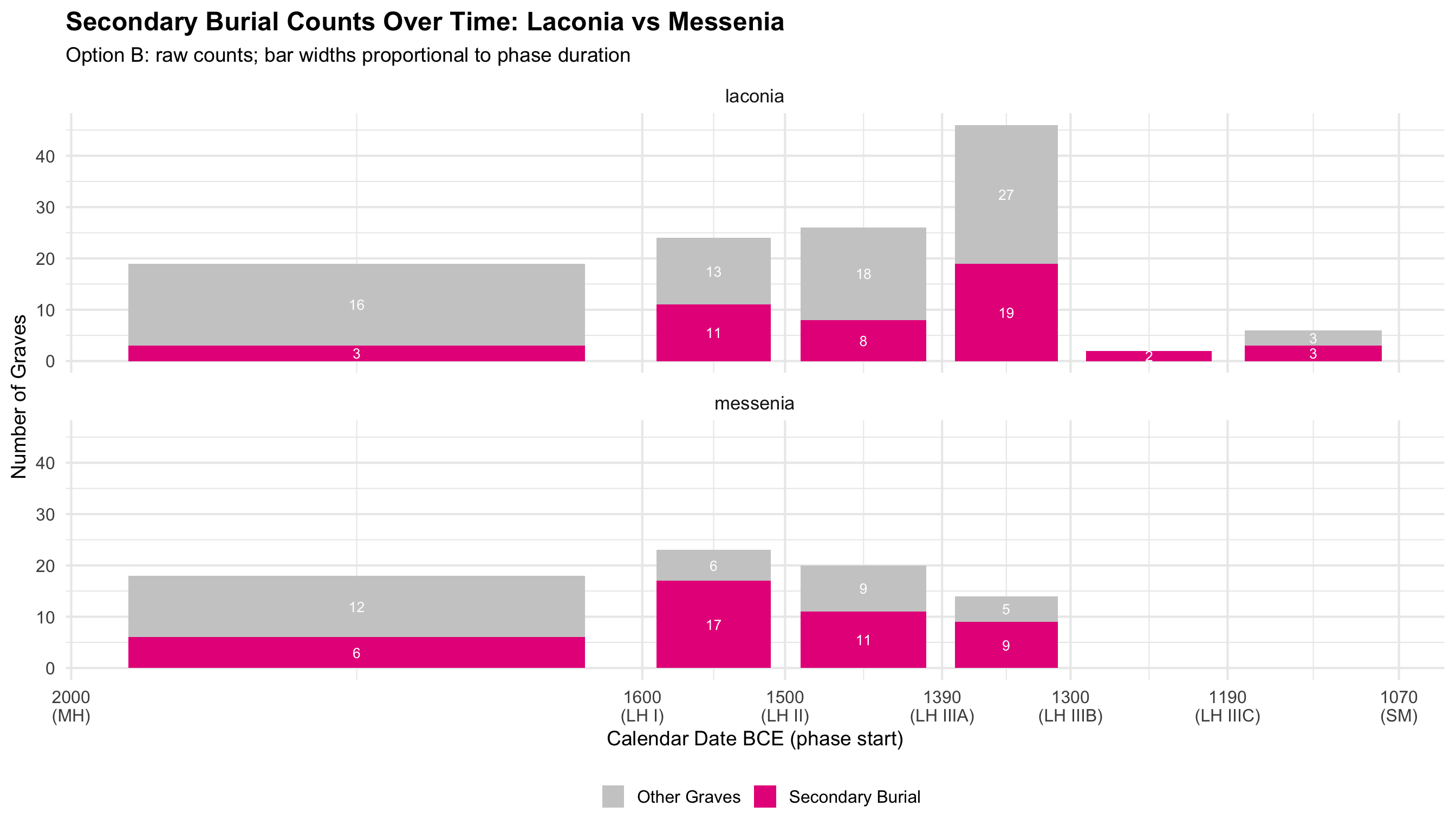
Option B: Raw Counts
secondary_raw_stack_b <- secondary_phase_b %>%
  mutate(n_other = n_graves - n_secondary) %>%
  pivot_longer(cols = c(n_secondary, n_other),
               names_to = "burial_type", values_to = "count") %>%
  mutate(burial_type = ifelse(burial_type == "n_secondary", "Secondary Burial", "Other Graves"))

ggplot(secondary_raw_stack_b,
       aes(x = phase_mid_bce, y = count, fill = burial_type, width = bar_width)) +
  geom_col(position = "stack") +
  geom_text(aes(label = ifelse(count > 0, count, "")),
            position = position_stack(vjust = 0.5), size = 3.5, color = "white") +
  scale_fill_manual(values = c("Secondary Burial" = colors$skulls, "Other Graves" = "grey80")) +
  scale_x_reverse(
    breaks = phase_cal$phase_start_bce,
    labels = paste0(phase_cal$phase_start_bce, "\n(", phase_cal$broad_phase, ")")
  ) +
  facet_wrap(~region, ncol = 1) +
  labs(
    title = "Secondary Burial Counts Over Time: Laconia vs Messenia",
    subtitle = "Option B: raw counts; bar widths proportional to phase duration",
    x = "Calendar Date BCE (phase start)", y = "Number of Graves", fill = ""
  ) +
  theme(legend.position = "bottom")
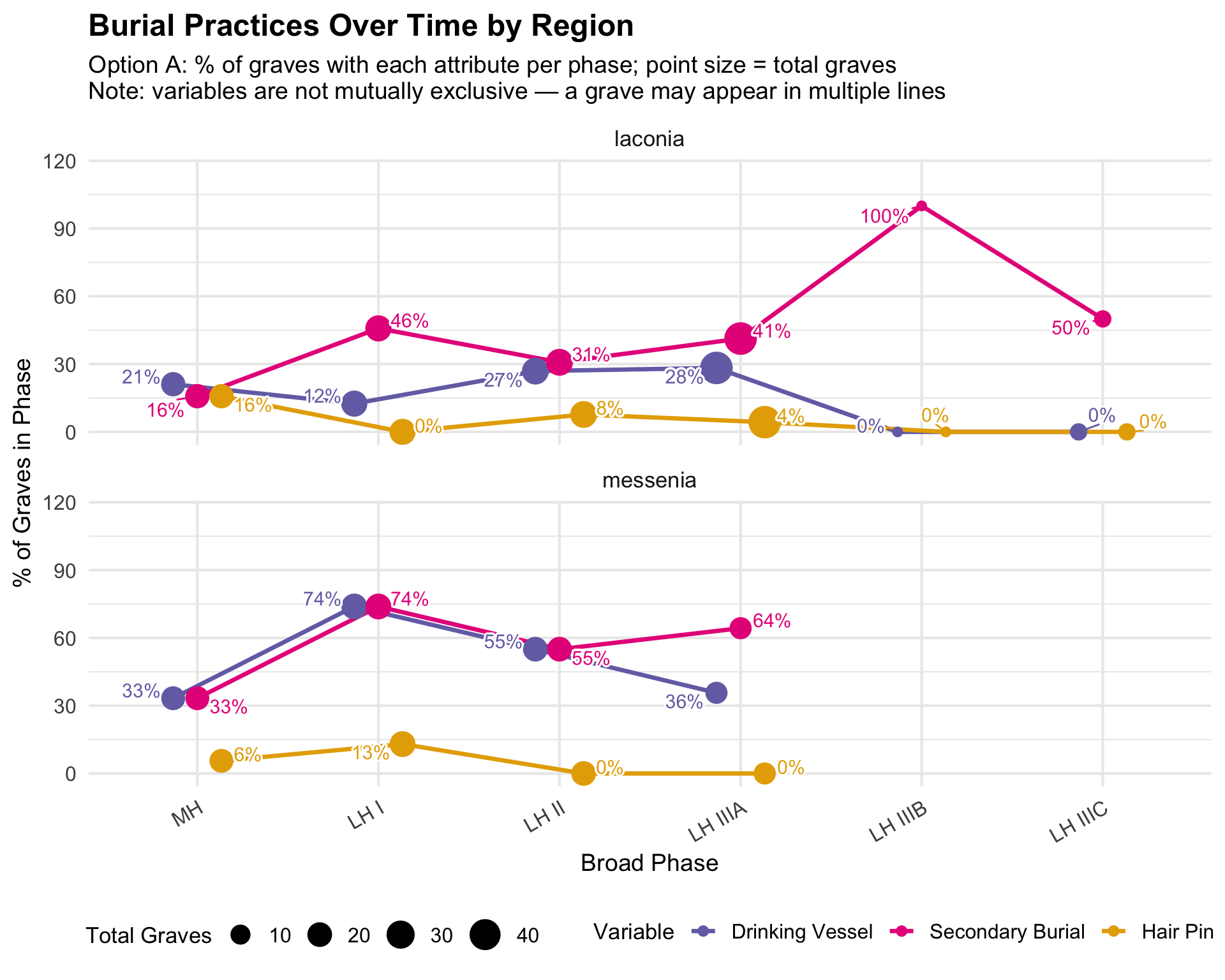
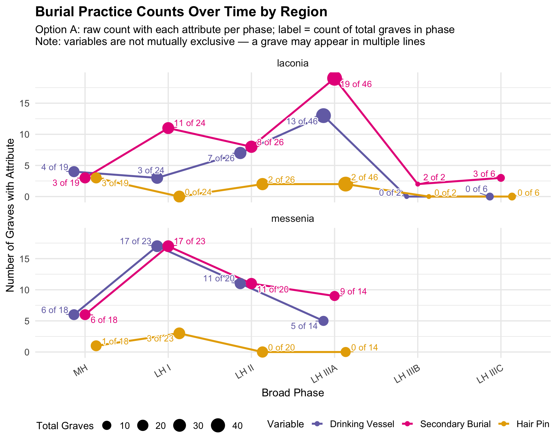
All Burial Variables Over Time
These line charts bring together the three main assemblage attributes
— drinking vessels, secondary burial, and hair pins — on a single
timeline, allowing comparison of their trends. Point size reflects the
total number of graves in that phase and region, so visually smaller
points signal phases with sparse data where percentages are less
reliable.
Important: The three variables are not
mutually exclusive — a grave may have drinking vessels
and secondary burial and a hair pin. The lines
therefore do not add up to 100%. Each line independently answers: “In
what share of graves in this phase is this attribute present?”
Excluded graves: Graves with NA for
broad_phase (unmatched period codes) are not plotted. This
is typically a small number; see the phase coverage table above.
Interpreting the raw count companion: The raw count
version makes the denominators visible. When a percentage looks high or
low, checking the raw counts reveals whether it is based on 2 graves or
20. Phases where total graves (point size) are very small should be
treated as preliminary observations, not firm patterns.
multi_phase_n_long <- multi_phase_data %>%
  pivot_longer(cols = c(n_drinking_vessel, n_secondary, n_pin),
               names_to = "variable", values_to = "count") %>%
  mutate(variable = case_when(
    variable == "n_drinking_vessel" ~ "Drinking Vessel",
    variable == "n_secondary"       ~ "Secondary Burial",
    variable == "n_pin"             ~ "Hair Pin"
  ),
  variable = factor(variable, levels = c("Drinking Vessel", "Secondary Burial", "Hair Pin")))

ggplot(multi_phase_n_long,
       aes(x = broad_phase, y = count, color = variable, group = variable)) +
  geom_line(linewidth = 1.2, position = dodge_a) +
  geom_point(aes(size = n_graves), position = dodge_a) +
  geom_text_repel(aes(label = paste0(count, " of ", n_graves)),
                  size = 4, show.legend = FALSE,
                  bg.color = "white", bg.r = 0.15,
                  min.segment.length = 0, seed = 42,
                  box.padding = 0.4,
                  position = dodge_a) +
  scale_color_manual(values = c(
    "Drinking Vessel"  = colors$drinking_vessel,
    "Secondary Burial" = colors$skulls,
    "Hair Pin"         = colors$pin
  )) +
  scale_size_continuous(range = c(2, 8)) +
  facet_wrap(~region, ncol = 1) +
  labs(
    title = "Burial Practice Counts Over Time by Region",
    subtitle = "Option A: raw count with each attribute per phase; label = count of total graves in phase\nNote: variables are not mutually exclusive — a grave may appear in multiple lines",
    x = "Broad Phase", y = "Number of Graves with Attribute",
    color = "Variable", size = "Total Graves"
  ) +
  theme(legend.position = "bottom", axis.text.x = element_text(angle = 30, hjust = 1))
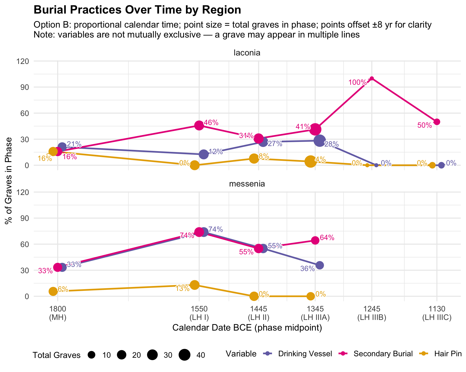
Option B: Proportional Calendar Time (BCE) — Proportions
multi_phase_b_pct <- multi_phase_pct_long %>%
  left_join(phase_cal, by = "broad_phase") %>%
  mutate(x_plot = phase_mid_bce + case_when(
    variable == "Drinking Vessel"  ~ -8L,
    variable == "Secondary Burial" ~  0L,
    variable == "Hair Pin"         ~  8L
  ))

ggplot(multi_phase_b_pct,
       aes(x = x_plot, y = percentage, color = variable, group = variable)) +
  geom_line(linewidth = 1.2) +
  geom_point(aes(size = n_graves)) +
  geom_text_repel(aes(label = paste0(round(percentage), "%")),
                  size = 4, show.legend = FALSE,
                  bg.color = "white", bg.r = 0.15,
                  min.segment.length = 0, seed = 42,
                  box.padding = 0.4) +
  scale_color_manual(values = c(
    "Drinking Vessel"  = colors$drinking_vessel,
    "Secondary Burial" = colors$skulls,
    "Hair Pin"         = colors$pin
  )) +
  scale_size_continuous(range = c(2, 8)) +
  scale_y_continuous(limits = c(0, 115)) +
  scale_x_reverse(
    breaks = phase_cal$phase_mid_bce,
    labels = paste0(phase_cal$phase_mid_bce, "\n(", phase_cal$broad_phase, ")")
  ) +
  facet_wrap(~region, ncol = 1) +
  labs(
    title = "Burial Practices Over Time by Region",
    subtitle = "Option B: proportional calendar time; point size = total graves in phase; points offset ±8 yr for clarity\nNote: variables are not mutually exclusive — a grave may appear in multiple lines",
    x = "Calendar Date BCE (phase midpoint)", y = "% of Graves in Phase",
    color = "Variable", size = "Total Graves"
  ) +
  theme(legend.position = "bottom")
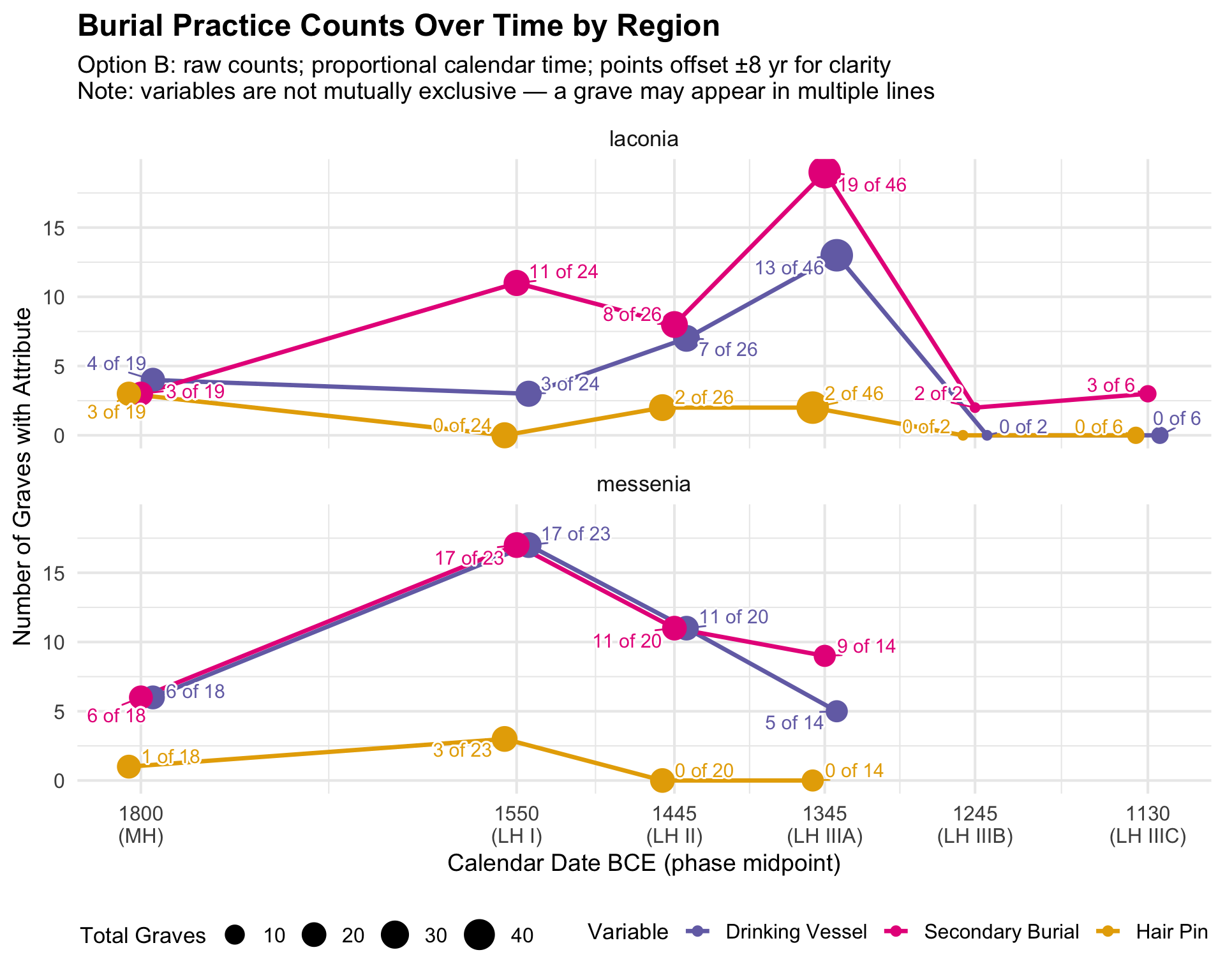
Option B: Raw Counts
multi_phase_b_n <- multi_phase_n_long %>%
  left_join(phase_cal, by = "broad_phase") %>%
  mutate(x_plot = phase_mid_bce + case_when(
    variable == "Drinking Vessel"  ~ -8L,
    variable == "Secondary Burial" ~  0L,
    variable == "Hair Pin"         ~  8L
  ))

ggplot(multi_phase_b_n,
       aes(x = x_plot, y = count, color = variable, group = variable)) +
  geom_line(linewidth = 1.2) +
  geom_point(aes(size = n_graves)) +
  geom_text_repel(aes(label = paste0(count, " of ", n_graves)),
                  size = 4, show.legend = FALSE,
                  bg.color = "white", bg.r = 0.15,
                  min.segment.length = 0, seed = 42,
                  box.padding = 0.4) +
  scale_color_manual(values = c(
    "Drinking Vessel"  = colors$drinking_vessel,
    "Secondary Burial" = colors$skulls,
    "Hair Pin"         = colors$pin
  )) +
  scale_size_continuous(range = c(2, 8)) +
  scale_x_reverse(
    breaks = phase_cal$phase_mid_bce,
    labels = paste0(phase_cal$phase_mid_bce, "\n(", phase_cal$broad_phase, ")")
  ) +
  facet_wrap(~region, ncol = 1) +
  labs(
    title = "Burial Practice Counts Over Time by Region",
    subtitle = "Option B: raw counts; proportional calendar time; points offset ±8 yr for clarity\nNote: variables are not mutually exclusive — a grave may appear in multiple lines",
    x = "Calendar Date BCE (phase midpoint)", y = "Number of Graves with Attribute",
    color = "Variable", size = "Total Graves"
  ) +
  theme(legend.position = "bottom")
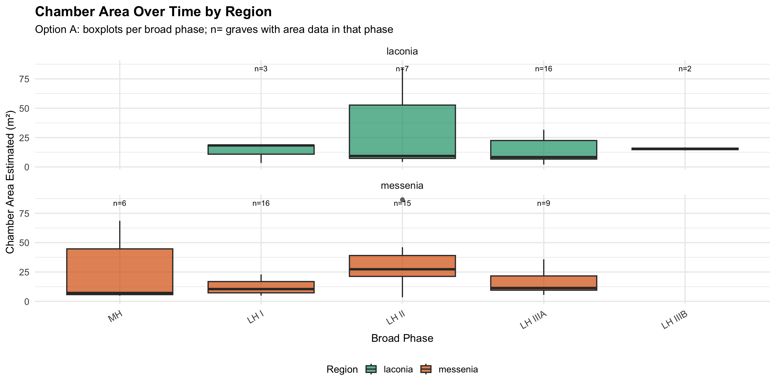
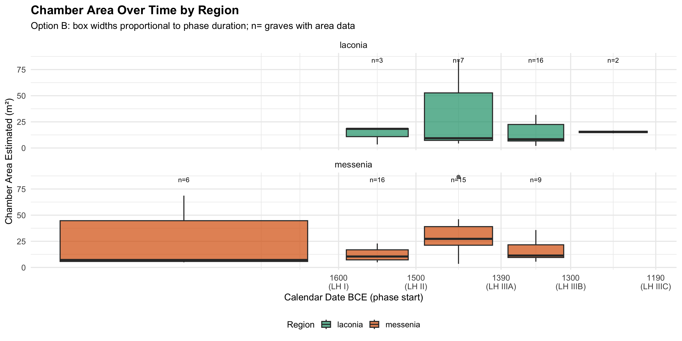
Chamber Area Over Time
These boxplots show whether the physical size of tomb
chambers changed over time within each region. Chamber area is
recorded in estimated square meters. Only graves with area data are
included — graves with NA for
area_of_chamber_estimated are excluded; n= labels show how
many graves contribute to each box. Phases with very few graves (n ≤ 3)
produce unreliable boxplots where the median and quartiles are heavily
influenced by individual outliers.
What to look for: An increase in median area over
time could suggest elaboration of tomb architecture; a decrease or
stasis might indicate continuity or economic contraction. Tomb type also
matters — tholos tombs tend to be larger than cist or pit graves — so
any apparent temporal trend should be considered alongside the tomb type
distribution of each phase.
Option A: Broad Phase Categories
area_phase_data <- cups_skulls_clean %>%
  dplyr::filter(!is.na(broad_phase) & !is.na(area_of_chamber_estimated))

area_n <- area_phase_data %>%
  group_by(region, broad_phase) %>%
  summarise(n = n(), .groups = "drop")

ggplot(area_phase_data, aes(x = broad_phase, y = area_of_chamber_estimated, fill = region)) +
  geom_boxplot(alpha = 0.7) +
  geom_text(data = area_n,
            aes(x = broad_phase, y = Inf, label = paste0("n=", n)),
            inherit.aes = FALSE, vjust = 2, size = 3.5) +
  scale_fill_manual(values = c(laconia = colors$laconia, messenia = colors$messenia)) +
  facet_wrap(~region, ncol = 1) +
  labs(
    title = "Chamber Area Over Time by Region",
    subtitle = "Option A: boxplots per broad phase; n= graves with area data in that phase",
    x = "Broad Phase", y = "Chamber Area Estimated (m\u00b2)", fill = "Region"
  ) +
  theme(legend.position = "bottom", axis.text.x = element_text(angle = 30, hjust = 1))
Option B: Proportional Calendar Time (BCE)
area_phase_b <- area_phase_data %>%
  left_join(phase_cal, by = "broad_phase")

area_n_b <- area_phase_b %>%
  group_by(region, broad_phase, phase_mid_bce) %>%
  summarise(n = n(), .groups = "drop")

ggplot(area_phase_b, aes(x = phase_mid_bce, y = area_of_chamber_estimated,
                          group = interaction(broad_phase, region), fill = region)) +
  geom_boxplot(aes(width = phase_duration * 0.8), alpha = 0.7) +
  geom_text(data = area_n_b,
            aes(x = phase_mid_bce, y = Inf, label = paste0("n=", n)),
            inherit.aes = FALSE, vjust = 2, size = 3.5) +
  scale_fill_manual(values = c(laconia = colors$laconia, messenia = colors$messenia)) +
  scale_x_reverse(
    breaks = phase_cal$phase_start_bce,
    labels = paste0(phase_cal$phase_start_bce, "\n(", phase_cal$broad_phase, ")")
  ) +
  facet_wrap(~region, ncol = 1) +
  labs(
    title = "Chamber Area Over Time by Region",
    subtitle = "Option B: box widths proportional to phase duration; n= graves with area data",
    x = "Calendar Date BCE (phase start)", y = "Chamber Area Estimated (m\u00b2)", fill = "Region"
  ) +
  theme(legend.position = "bottom")
burial_counts <- cups_skulls_clean %>%
  count(burial_category) %>%
  arrange(desc(n))
for (i in 1:nrow(burial_counts)) {
  cat("   -", burial_counts$burial_category[i], ":", burial_counts$n[i], "graves\n")
}
   - Unknown/Not Recorded : 100 graves
   - Primary Only : 78 graves
   - Secondary Only : 61 graves
   - Both Primary & Secondary : 57 graves
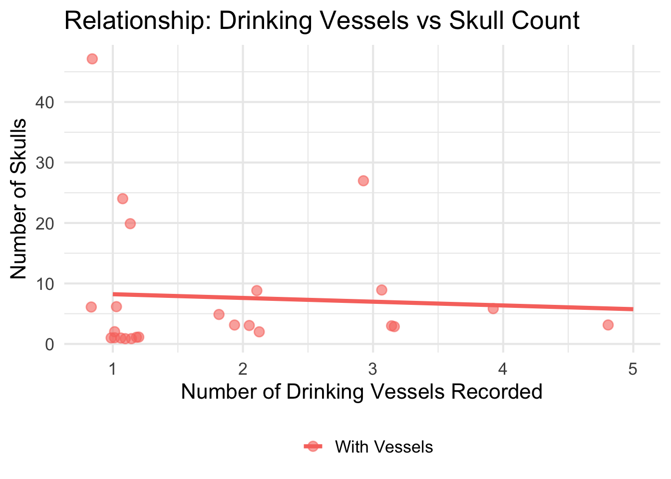
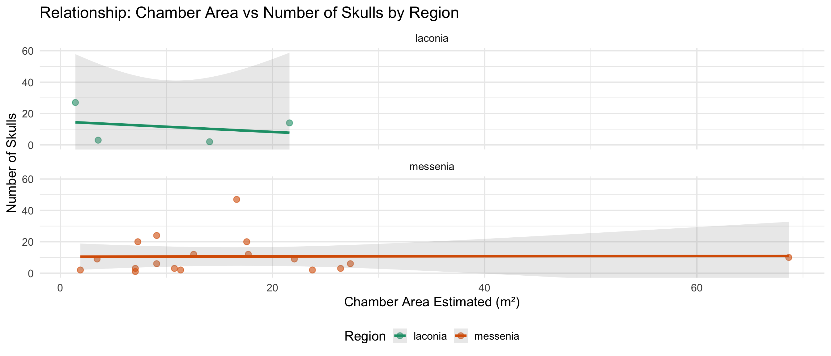
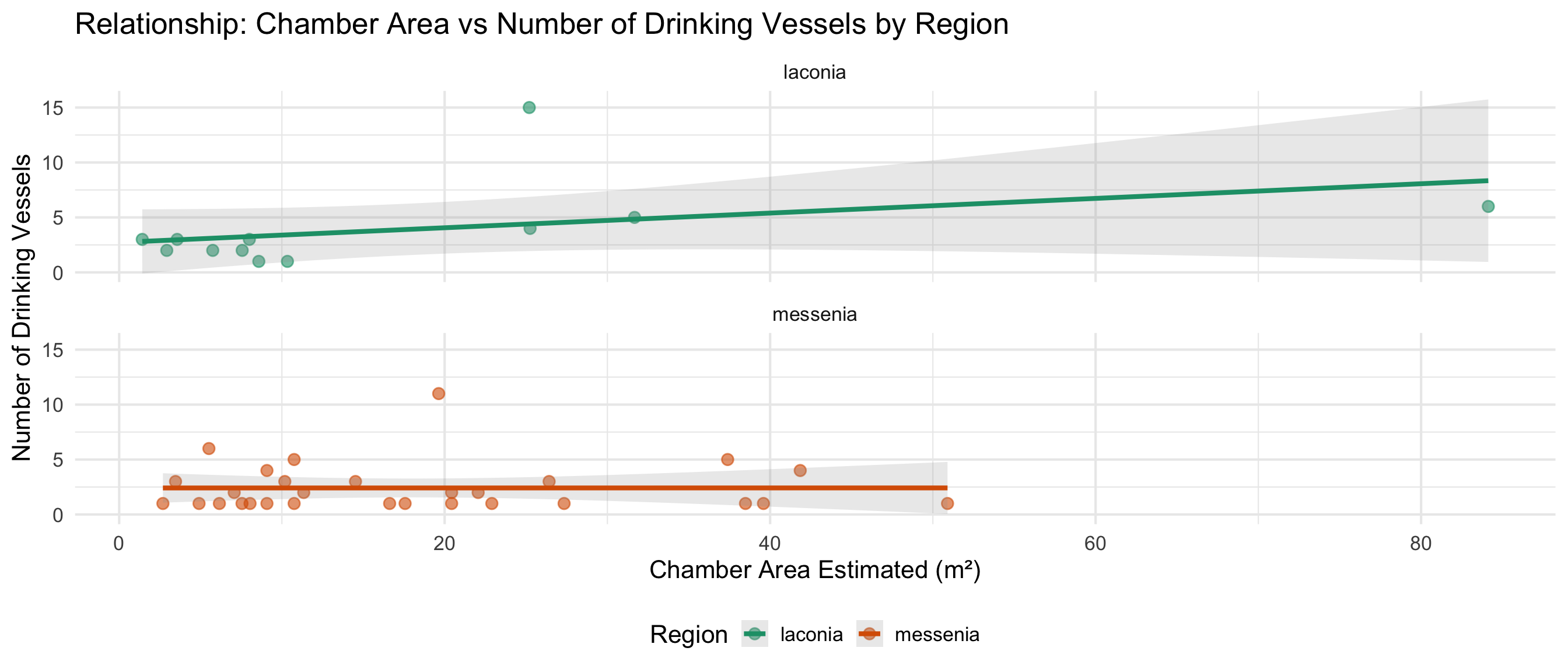
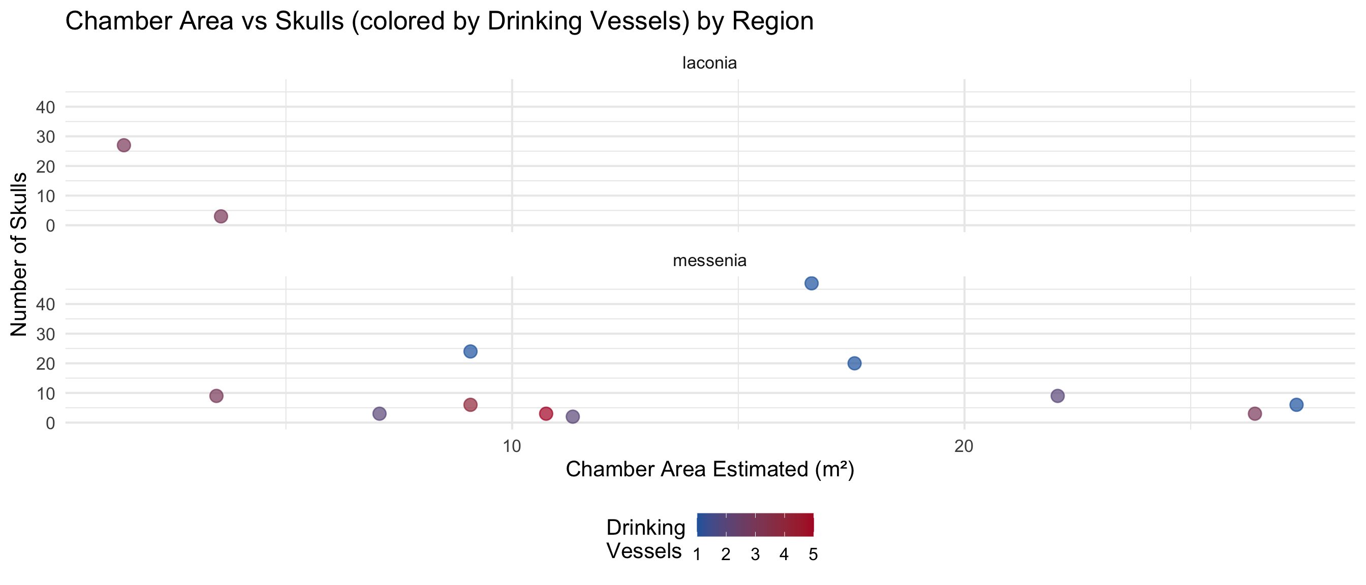
Chamber Space and Burial Goods
Do larger chambers have more skulls and drinking vessels?
This section explores whether the estimated chamber area relates to
the number of skulls and drinking vessels found.
HOW YOUR PERIOD DICTIONARY WILL ENHANCE THIS: - Once
you complete period_dictionary.csv and enable the
dictionary loading code, we can add temporal layers - You’ll be able to
see if these relationships change across periods - Time-based patterns
can reveal ritual practice evolution
Data Availability
space_analysis_data <- cups_skulls_clean %>%
  dplyr::filter(!is.na(area_of_chamber_estimated))

cat("Graves with chamber area estimated:", nrow(space_analysis_data), "\n")
Graves with chamber area estimated: 99
cat("Graves with area AND skull count:", sum(!is.na(space_analysis_data$skulls_number)), "\n")
Graves with area AND skull count: 22
cat("Graves with area AND vessel count:", sum(!is.na(space_analysis_data$drinking_vessel_number)), "\n\n")
Graves with area AND vessel count: 41
# Summary statistics for chamber area
cat("Chamber Area Summary (m²):\n")