DE Analysis
Ha Tran
22/08/2021
Last updated: 2022-11-05
Checks: 7 0
Knit directory: SRB_2022/1_analysis/
This reproducible R Markdown analysis was created with workflowr (version 1.7.0). The Checks tab describes the reproducibility checks that were applied when the results were created. The Past versions tab lists the development history.
Great! Since the R Markdown file has been committed to the Git repository, you know the exact version of the code that produced these results.
Great job! The global environment was empty. Objects defined in the global environment can affect the analysis in your R Markdown file in unknown ways. For reproduciblity it’s best to always run the code in an empty environment.
The command set.seed(12345) was run prior to running the
code in the R Markdown file. Setting a seed ensures that any results
that rely on randomness, e.g. subsampling or permutations, are
reproducible.
Great job! Recording the operating system, R version, and package versions is critical for reproducibility.
Nice! There were no cached chunks for this analysis, so you can be confident that you successfully produced the results during this run.
Great job! Using relative paths to the files within your workflowr project makes it easier to run your code on other machines.
Great! You are using Git for version control. Tracking code development and connecting the code version to the results is critical for reproducibility.
The results in this page were generated with repository version cc4bf5d. See the Past versions tab to see a history of the changes made to the R Markdown and HTML files.
Note that you need to be careful to ensure that all relevant files for
the analysis have been committed to Git prior to generating the results
(you can use wflow_publish or
wflow_git_commit). workflowr only checks the R Markdown
file, but you know if there are other scripts or data files that it
depends on. Below is the status of the Git repository when the results
were generated:
Ignored files:
    Ignored:    .Rhistory
    Ignored:    .Rproj.user/

Untracked files:
    Untracked:  .gitignore
    Untracked:  0_data/
    Untracked:  1_analysis/
    Untracked:  3_output/
    Untracked:  LICENSE.md
    Untracked:  README.md
    Untracked:  SRB_2022.Rproj
Note that any generated files, e.g. HTML, png, CSS, etc., are not included in this status report because it is ok for generated content to have uncommitted changes.
There are no past versions. Publish this analysis with
wflow_publish() to start tracking its development.
Data Setup
# working with data
library(dplyr)
library(magrittr)
library(readr)
library(tibble)
library(reshape2)
library(tidyverse)

# Visualisation:
library(kableExtra)
library(ggplot2)
library(grid)
library(pander)
library(cowplot)
library(pheatmap)

# Custom ggplot
library(ggplotify)
library(ggpubr)
library(ggrepel)
library(viridis)

# Bioconductor packages:
library(edgeR)
library(limma)
library(Glimma)

theme_set(theme_minimal())
pub <- readRDS(here::here("0_data/RDS_objects/pub.rds"))
Import DGElist Data
DGElist object containing the raw feature count, sample metadata, and gene metadata, created in the Set Up stage.
# load DGElist previously created in the set up
dge <- readRDS(here::here("0_data/RDS_objects/dge.rds"))
Differential Gene Expression Analysis
Initial Parameterisation
The varying methods used to identify differential expression all rely on similar initial parameters. These include:
- The Design Matrix,
- Estimation of Dispersion, and
- Contrast Matrix
Design Matrix
The experimental design can be parameterised in a one-way layout where one coefficient is assigned to each group. The design matrix formulated below contains the predictors of each sample
# null design with unit vector for generation of voomWithQualityWeights downstream
null_design <- matrix(1, ncol = 1, nrow = ncol(dge))

# setup full design matrix with sample_group
full_design <- model.matrix(~ 0 + group,
  data = dge$samples)

# remove "sample_group" from each column names
colnames(full_design) <- gsub(
  "group",
  "",
  colnames(full_design))
Contrast Matrix
The contrast matrix is required to provide a coefficient to each comparison and later used to test for significant differential expression with each comparison group
contrast <- limma::makeContrasts(
  INTvsCONT = INT - CONT,
  levels = full_design)

colnames(contrast) <- c("INT vs CONT")
Limma-Voom
Apply voom transformation
Voom is used to estimate the mean-variance relationship of the data, which is then used to calculate and assign a precision weight for each of the observation (gene). This observational level weights are then used in a linear modelling process to adjust for heteroscedasticity. Log count (logCPM) data typically show a decreasing mean-variance trend with increasing count size (expression).
However, for some dataset with potential sample outliers,
voomWithQualityWeights can be used to calculate
sample-specific quality weights. The application of observational and
sample-specific weights can objectively and systematically correct for
outliers and better than manually removing samples in cases where there
are no clear-cut reasons for replicate variations
Voom with observational-level weights
# voom tranformation without sample weights
voom <- limma::voom(counts = dge, design = full_design, plot = TRUE,)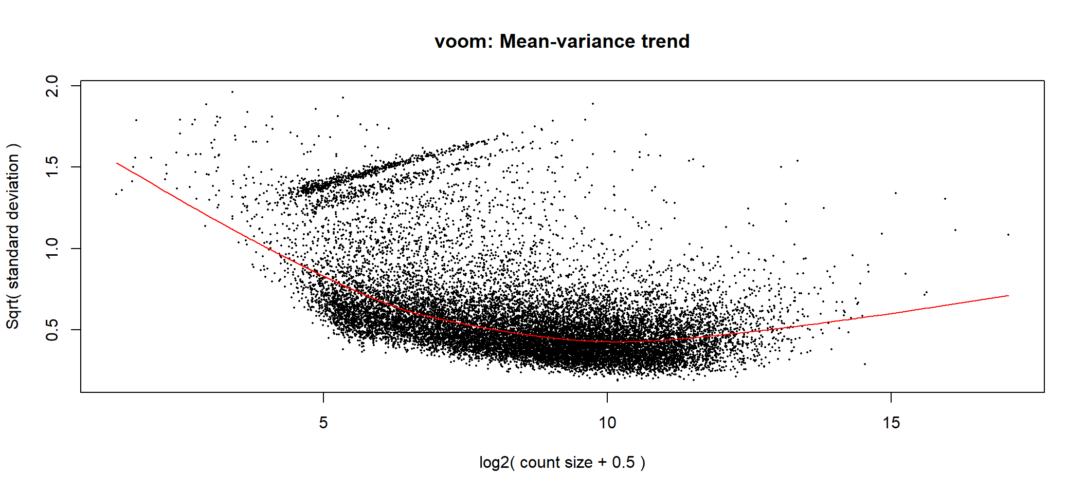
Voom transformation with observational weights
Voom with observational and group level weights
# voom transformation with sample weights using full_design matrix for group-specific weights
voom1 <- limma::voomWithQualityWeights(counts = dge, design = full_design, plot = TRUE)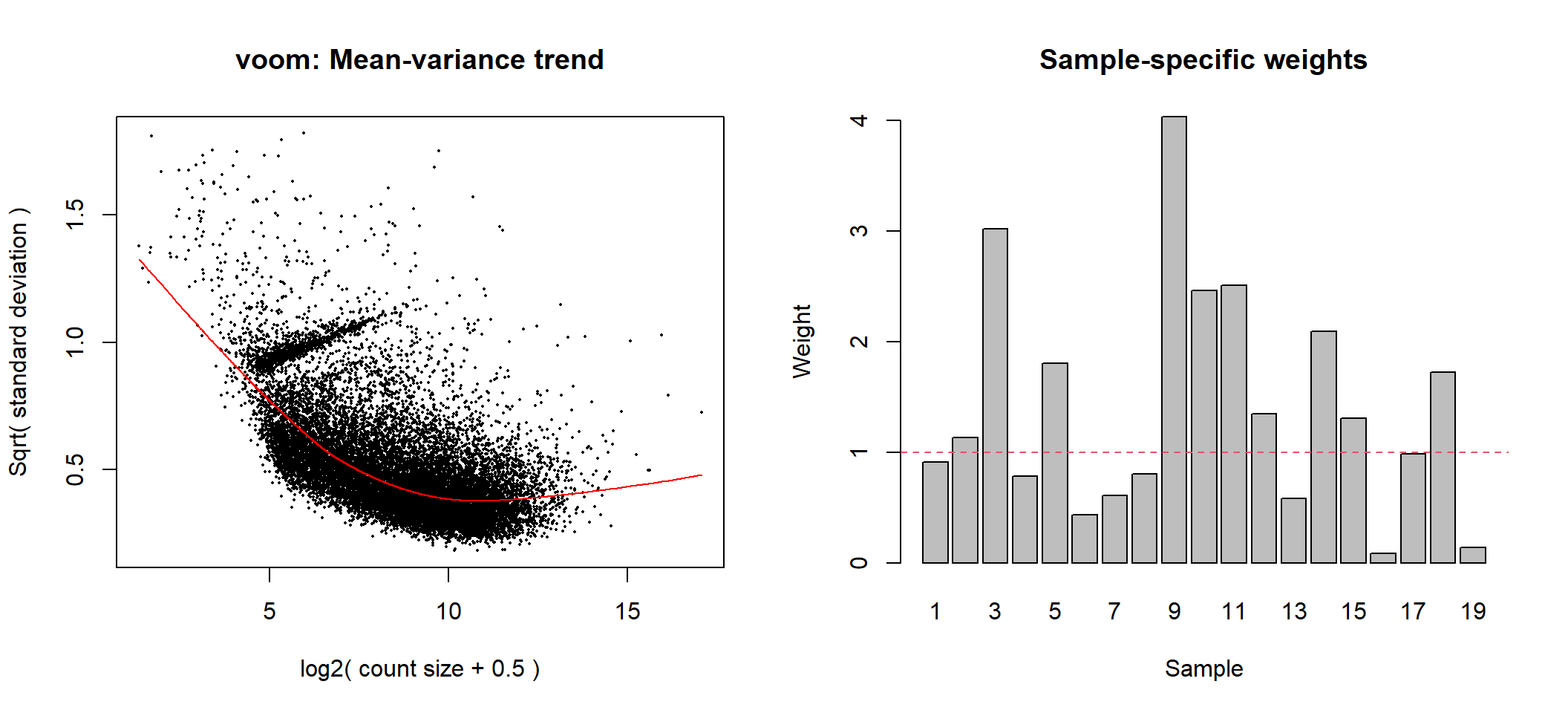
Voom transformation with observational and group-specific weights
Voom with observational and sample level weights
# voom transformation with sample weights using null design matrix
voom2 <- limma::voomWithQualityWeights(counts = dge,design = null_design, plot = TRUE)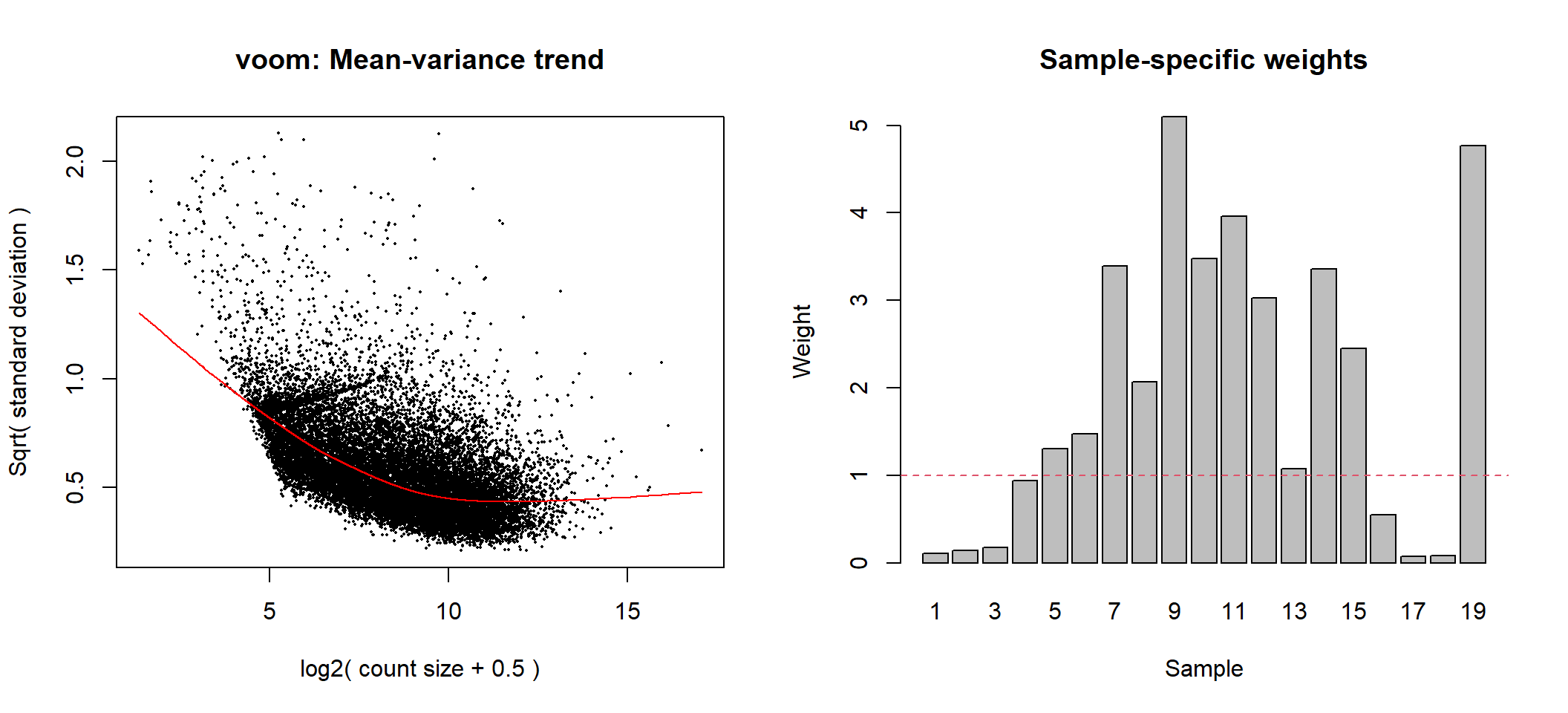
Voom transformation with observational and sample-specific weights
Apply linear model
# specifying FC of interest
options(digits = 6)
fc <- c(1.05, 1.1, 1.5)
lfc <- log(x = fc, 2)
Without TREAT
# function for applying linear model, generate decideTest table, and extract topTable
limmaFit_ebayes <- function(x, adjMethod, p.val){
  lm <- limma::lmFit(object = x, design = full_design) %>%
    contrasts.fit(contrasts = contrast) %>%
    limma::eBayes()

  lm_dt <- decideTests(object = lm, adjust.method = adjMethod, p.value = p.val)
  print(knitr::kable(summary(lm_dt)
                      , caption = paste0("Number of significant DE genes from '", deparse(substitute(x)), "' with '", adjMethod, "' adjusment method, and at a p-value/adj.p-value of ", p.val)) %>%
    kable_styling(bootstrap_options = c("striped", "hover")))

  lm_all <- lapply(1:ncol(lm), function(y){
    limma::topTable(lm, coef = y, number = Inf, adjust.method = adjMethod) %>%
      dplyr::select(c("gene", "gene_name", "gene_biotype", "logFC", "AveExpr", "P.Value", "adj.P.Val", "description", "entrezid"))
    })
  names(lm_all) <- as.data.frame(contrast) %>% colnames()
  return(lm_all)
}

lm_voom1_pval0.01 <- limmaFit_ebayes(x = voom1, adjMethod = "none", p.val = 0.01)| INT vs CONT | |
|---|---|
| Down | 4583 |
| NotSig | 7985 |
| Up | 4654 |
lm_voom2_pval0.01 <- limmaFit_ebayes(x = voom2, adjMethod = "none", p.val = 0.01)| INT vs CONT | |
|---|---|
| Down | 305 |
| NotSig | 14943 |
| Up | 1974 |
lm_voom2_fdr0.7 <- limmaFit_ebayes(x = voom2, adjMethod = "fdr", p.val = 0.7)| INT vs CONT | |
|---|---|
| Down | 5931 |
| NotSig | 5349 |
| Up | 5942 |
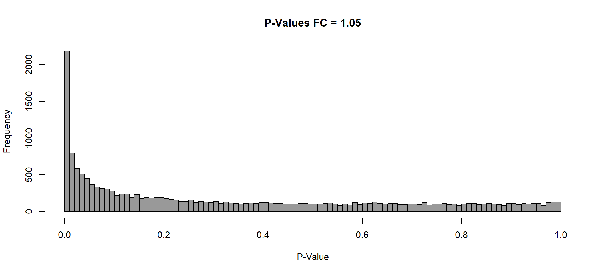
TREAT FC=1.05
limmaFit_treat <- function(x, fc, adjMethod, p.val){
  lm_treat <- limma::lmFit(object = x, design = full_design) %>%
    contrasts.fit(contrasts = contrast) %>%
    limma::treat(fc = fc)

  lm_treat_dt <- decideTests(object = lm_treat, adjust.method = adjMethod, p.value = p.val)
  print(knitr::kable(summary(lm_treat_dt),
                     caption = paste0("Number of DE genes significantly above a FC of ", fc, " from '", deparse(substitute(x)), "' with '", adjMethod, "' adjusment method, and at a p-value/adj.p-value of ", p.val)) %>%
    kable_styling(bootstrap_options = c("striped", "hover")))

  lm_treat_all <- lapply(1:ncol(lm_treat), function(y){
    limma::topTreat(lm_treat, coef = y, number = Inf, adjust.method = adjMethod) %>%
      dplyr::select(c("gene", "gene_name", "gene_biotype", "logFC", "AveExpr", "P.Value", "adj.P.Val", "description", "entrezid"))
    })
  names(lm_treat_all) <- as.data.frame(contrast) %>% colnames()
  return(lm_treat_all)
}

assign(paste0("lmTreat_fc", fc[1], "_voom2_fdr0.05"),
limmaFit_treat(x = voom2, fc = fc[1], adjMethod = "fdr", p.val = 0.05))| INT vs CONT | |
|---|---|
| Down | 95 |
| NotSig | 15593 |
| Up | 1534 |
assign(paste0("lmTreat_fc", fc[1], "_voom2_pval0.01"),
limmaFit_treat(x = voom2, fc = fc[1], adjMethod = "none", p.val = 0.01))| INT vs CONT | |
|---|---|
| Down | 260 |
| NotSig | 15041 |
| Up | 1921 |
assign(paste0("lmTreat_fc", fc[1], "_voom2_pval0.05"),
limmaFit_treat(x = voom2, fc = fc[1], adjMethod = "none", p.val = 0.05))| INT vs CONT | |
|---|---|
| Down | 1443 |
| NotSig | 12700 |
| Up | 3079 |
### Old code used to interatively generate lmTreat dataset with different fc cutoff
## with treat
lmTreat <- list()
lmTreat_dt <- list()
lmTreat_all <- list()
lmTreat_sig <- list()

for (i in 1:length(fc)) {
  x <- fc[i] %>% as.character()
  lmTreat[[x]] <- limma::lmFit(object = voom2, design = full_design) %>%
    limma::contrasts.fit(contrasts = contrast) %>%
    limma::treat(lfc = lfc[i])

  # decide test, do before taking topTreat, as input need to be MArraryLM list
  lmTreat_dt[[x]] <- decideTests(lmTreat[[x]], adjust.methods = "fdr", p.value = 0.05)

  # extract a table of genes from a linear model fit, export and used for downstream analysis
  lmTreat_all[[x]] <- topTreat(fit = lmTreat[[x]], coef = 1, number = Inf, adjust.method = "fdr") %>%
    dplyr::select(c("gene_name", "logFC", "AveExpr", "P.Value", "adj.P.Val", "description", "entrezid"))

  # extract a table of significant genes from a linear model fit, export and used for downstream analysis
  lmTreat_sig[[x]] <- topTreat(fit = lmTreat[[x]], coef = 1, number = Inf, adjust.method = "fdr", p.value = 0.05) %>%
    dplyr::select(c("gene_name", "logFC", "AveExpr", "P.Value", "adj.P.Val", "description", "entrezid"))
}
INT vs CONT Visualisation
P Value histogram
lmTreat_hist <- list()
for (i in 1:length(fc)) {
  x <- fc[i] %>% as.character()
  lmTreat_hist[[x]] <- hist(x = lmTreat[[x]]$p.value, breaks = 100, plot = F)
}
plot(
  x = lmTreat_hist[[1]],
  main = paste0("P-Values FC = ", fc[[1]]),
  xlab = "P-Value",
  col = "gray60"
)
invisible(dev.print(svg, here::here(paste0("2_plots/de/pval_", fc[1], ".svg"))))MA Plot
ma <- list()
for (i in 1:length(fc)) {
  x <- fc[i] %>% as.character()

  # add an extra column and determine whether the DE genes are significant
  lmTreat_all[[x]] <- lmTreat_all[[x]] %>%
    as.data.frame() %>%
    dplyr::mutate(Expression = case_when(
      adj.P.Val <= 0.05 & logFC >= lfc ~ "Up-regulated",
      adj.P.Val <= 0.05 & logFC <= -lfc ~ "Down-regulated",
      TRUE ~ "Insignificant"
    ))

  # adding labels to top genes
  top <- 3
  top_limma <- bind_rows(
    lmTreat_all[[x]] %>%
      dplyr::filter(Expression == "Up-regulated") %>%
      arrange(adj.P.Val, desc(abs(logFC))) %>%
      head(top),
    lmTreat_all[[x]] %>%
      dplyr::filter(Expression == "Down-regulated") %>%
      arrange(adj.P.Val, desc(abs(logFC))) %>%
      head(top)
  )
  invisible(top_limma %>% as.data.frame())

  ma[[x]] <- lmTreat_all[[x]] %>%
    ggplot(aes(x = AveExpr, y = logFC)) +
    geom_point(aes(colour = Expression),

      ### PUBLISH
      size = 0.3,
      # alpha = 0.7,
      show.legend = T
    ) +
    # geom_label_repel(
    #   data = top_limma,
    #   mapping = aes(x = AveExpr, logFC, label = gene_name),
    #
    #   ### PUBLISH
    #   size = 1.7,
    #   label.padding = 0.15,
    #   # label.r = 0.15,
    #   box.padding = 0.15
    #   # point.padding = 0.2
    # ) +
    geom_hline(yintercept = c(-fc[i], 0, fc[i]), linetype = c("dashed", "solid", "dashed")) +

    ### PUBLISH
    ylim(-8, 8) +
    theme(legend.position = "bottom",
          legend.box.margin = margin(-10,0,0,0),
          legend.key.size = unit(0, "lines")
          )+

    xlab(expression("log"[2] * "CPM")) +
    ylab(expression("log"[2] * "FC")) +
    scale_fill_manual(values = c("dodgerblue3", alpha(colour = "gray80", alpha = 0.9), "firebrick3")) +
    scale_color_manual(labels = c(paste0("Down: ", sum(lmTreat_all[[x]]$Expression == "Down-regulated"), "  "),
                                  paste0("NS: ", sum(lmTreat_all[[x]]$Expression == "Insignificant"), "  "),
                                  paste0("Up: ", sum(lmTreat_all[[x]]$Expression == "Up-regulated"), " ")),
                       values = c("dodgerblue3", alpha(colour = "gray80", alpha = 0.6), "firebrick3")) +

    guides(colour = guide_legend(override.aes = list(size = 1.5))) +
    labs(
      # title = "MA Plot: LIMMA-VOOM + TREAT",
      # subtitle = "Intact vs Control",
      colour = "Expression")

  # save to directory
  ggsave(paste0("ma_", fc[i], ".png"),
    plot = ma[[x]],
    path = here::here("2_plots/de/"),

    ### PUBLISH
    width = 58,
    height = 70,
    units = "mm"
  )
}

# display
ma[[1]]
Volcano Plot
vol <- list()
for (i in 1:length(fc)) {
  x <- fc[i] %>% as.character()

  # adding labels to top genes
  top <- 3
  top_limma <- bind_rows(
    lmTreat_all[[x]] %>%
      dplyr::filter(Expression == "Up-regulated") %>%
      arrange(adj.P.Val, desc(abs(logFC))) %>%
      head(top),
    lmTreat_all[[x]] %>%
      dplyr::filter(Expression == "Down-regulated") %>%
      arrange(adj.P.Val, desc(abs(logFC))) %>%
      head(top)
  )
  invisible(top_limma %>% as.data.frame())

  # generate vol plot with the allDEgene data.frame
  vol[[x]] <- lmTreat_all[[x]] %>%
    ggplot(aes(
      x = logFC,
      y = -log(adj.P.Val, 10)
    )) +
    geom_point(aes(colour = Expression),

      ### PUBLISH
      size = 0.3,
      # alpha = 0.8,
      show.legend = T
    ) +
    # geom_label_repel(
    #   data = top_limma,
    #   mapping = aes(logFC, -log(adj.P.Val, 10), label = gene_name),
    #
    #   ### PUBLISH
    #   size = 1.7,
    #   label.padding = 0.15,
    #   # label.r = 0.15,
    #   box.padding = 0.15
    #   # point.padding = 0.2
    # ) +

    ### PUBLISH
    xlim(-8.15, 8.15)+
    theme(legend.position = "bottom",
          legend.box.margin = margin(-10,0,0,0),
          legend.key.size = unit(0, "lines")
          )+

    xlab(expression("log"[2] * "FC")) +
    ylab(expression("-log"[10] * "FDR")) +
    scale_fill_manual(values = c("dodgerblue3", alpha(colour = "gray80", alpha = 0.9), "firebrick3")) +
    scale_color_manual(labels = c(paste0("Down: ", sum(lmTreat_all[[x]]$Expression == "Down-regulated"), "  "),
                                  paste0("NS: ", sum(lmTreat_all[[x]]$Expression == "Insignificant"), "  "),
                                  paste0("Up: ", sum(lmTreat_all[[x]]$Expression == "Up-regulated"), " ")),
                       values = c("dodgerblue3", alpha(colour = "gray80", alpha = 0.6), "firebrick3")) +

    guides(colour = guide_legend(override.aes = list(size = 1.5))) +
    labs(

      ### PUBLISH
      # title = "Volcano Plot: LIMMA-VOOM + TREAT",
      # subtitle = "Intact vs Control",
      colour = "Expression"
    )

  # save to directory
  ggsave(paste0("vol_", fc[i], ".png"),
    plot = vol[[x]],
    path = here::here("2_plots/de/"),

    ### PUBLISH
    width = 58,
    height = 70,
    units = "mm"
  )
}

# display
vol[[1]]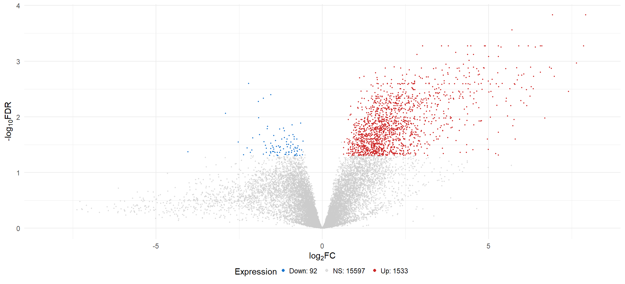
Top Upregulated
# create df with normalised read counts with an additional entrezid column for binding
logCPM <- cpm(dge, prior.count = 3, log = TRUE) %>% subset(select = 1:7)
rownames(logCPM) <- dge$genes$gene_name
# colnames(logCPM) <- c("Control 1", "Control 2", "Control 4", "Intact 1", "Intact 2", "Intact 3", "Intact 4")

# colour palette for heatmap
my_palette <- colorRampPalette(c("dodgerblue3", "white", "firebrick3"))(n = 201)

# df for heatmap annotation of sample group
anno <- as.factor(dge$samples$group) %>% as.data.frame() %>% dplyr::slice(1:7)
colnames(anno) <- "Sample Groups"
anno$`Sample Groups` <- gsub("CONT", "Control", anno$`Sample Groups`)
anno$`Sample Groups` <- gsub("INT", "Intact", anno$`Sample Groups`)
rownames(anno) <- colnames(logCPM)

# setting colour of sample group annotation
anno_colours <- c("#f8766d", "#00bdc4")
names(anno_colours) <- c("Control", "Intact")

logCPM_up=list()
logCPM_down=list()
for (i in 1:length(fc)) {
  x <- fc[i] %>% as.character()

  # filtering top upregulated genes then filter the logCPM values of those genes.
  upReg <- lmTreat_sig[[x]] %>%
    dplyr::filter(logFC > 0) %>%
    arrange(sort(adj.P.Val, decreasing = F))
  upReg <- upReg[1:20,]
  logCPM_up[[x]] <- logCPM[upReg$gene_name,] %>% as.data.frame()


  # filtering top upregulated genes then filter the logCPM values of those genes.
  downReg <- lmTreat_sig[[x]] %>%
    dplyr::filter(logFC < 0) %>%
    arrange(sort(adj.P.Val, decreasing = F))
  if (nrow(downReg) >= 20) {max <-  20} else {max <-  nrow(downReg)}
  downReg <- downReg[1:max,]
  logCPM_down[[x]] <- logCPM[downReg$gene_name,] %>% as.data.frame()
}
heat_up=list()
for (i in 1:length(fc)) {
x <- fc[i] %>% as.character()
heat_up[[x]] <-
pheatmap(
mat = logCPM_up[[x]],
### Publish
show_colnames = F,
main = paste0("Top ", nrow(logCPM_up[[x]]), " significant upregulated genes\n"),
legend = F,
annotation_legend = T,
fontsize = 8,
fontsize_col = 9,
fontsize_number = 7,
fontsize_row = 8,
treeheight_row = 25,
treeheight_col = 10,
clustering_distance_rows = "euclidean",
legend_breaks = c(seq(-3, 11, by = .5), 1.3),
legend_labels = c(seq(-3, 11, by = .5), "Z-Score"),
angle_col = 90,
cutree_cols = 2,
cutree_rows = 1,
border_color = NA,
color = viridis_pal(option = "viridis")(300),
scale = "row",
annotation_col = anno,
annotation_colors = list("Sample Groups" = anno_colours),
annotation_names_col = F,
annotation = T,
silent = T,
labels_row = as.expression(lapply(rownames(logCPM_up[[x]]), function(a) bquote(italic(.(a)))))
) %>% as.ggplot()
# save to directory
ggsave(paste0("heat_up_", fc[i], ".svg"),
plot = heat_up[[x]],
path = here::here("2_plots/de/"),
### PUBLISH
width = 112,
height = 110,
units = "mm"
)
}
heat_up[[1]] 
Top Downregulated
heat_down=list()
for (i in 1:length(fc)) {
  x <- fc[i] %>% as.character()
  heat_down[[x]] <-
    pheatmap(
      mat = logCPM_down[[x]],

      ### Publish
      show_colnames = F,
      main = paste0("Top ", nrow(logCPM_down[[x]]), " significant downregulated genes\n"),
      legend = F,
      annotation_legend = T,
      fontsize = 8,
      fontsize_col = 9,
      fontsize_number = 7,
      fontsize_row = 8,
      treeheight_row = 25,
      treeheight_col = 10,
      clustering_distance_rows = "euclidean",
      legend_breaks = c(seq(-3, 11, by = .5), 1.3),
      legend_labels = c(seq(-3, 11, by = .5), "Z-Score"),
      angle_col = 90,
      cutree_cols = 2,
      cutree_rows = 1,
      border_color = NA,
      color = viridis_pal(option = "viridis")(300),
      scale = "row",
      annotation_col = anno,
      annotation_colors = list("Sample Groups" = anno_colours),
      annotation_names_col = F,
      annotation = T,
      silent = T,

      labels_row = as.expression(lapply(rownames(logCPM_down[[x]]), function(a) bquote(italic(.(a)))))

  ) %>% as.ggplot()

# save to directory
  ggsave(paste0("heat_down_", fc[i], ".svg"),
    plot = heat_down[[x]],
    path = here::here("2_plots/de/"),

    ### PUBLISH
    width = 112,
    height = 110,
    units = "mm"
  )
}

heat_down[[1]] 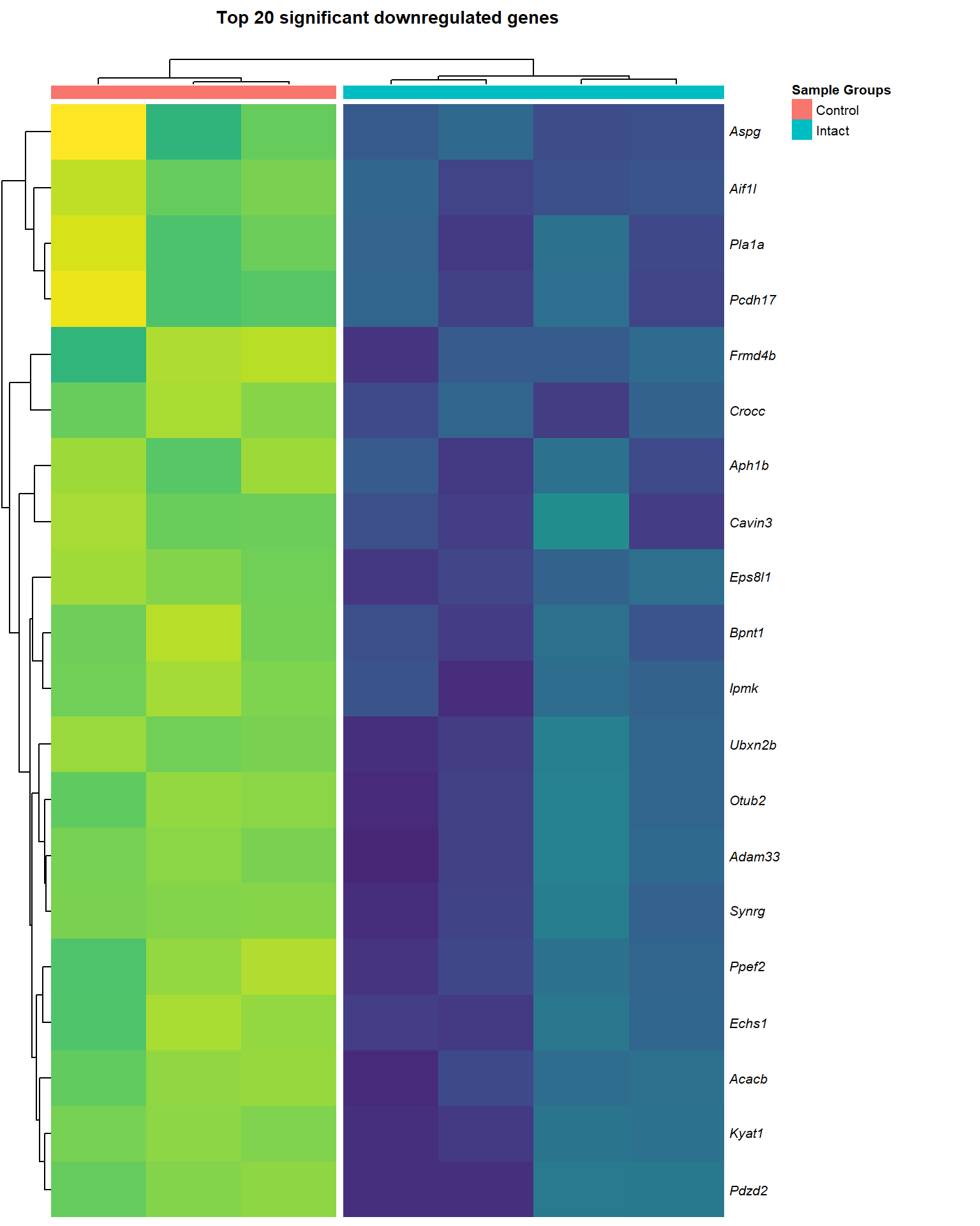
TREAT FC=1.1
assign(paste0("lmTreat_fc", fc[2], "_voom2_fdr0.05"),
limmaFit_treat(x = voom2, fc = fc[2], adjMethod = "fdr", p.val = 0.05))| INT vs CONT | |
|---|---|
| Down | 55 |
| NotSig | 15775 |
| Up | 1392 |
assign(paste0("lmTreat_fc", fc[2], "_voom2_pval0.01"),
limmaFit_treat(x = voom2, fc = fc[2], adjMethod = "none", p.val = 0.01))| INT vs CONT | |
|---|---|
| Down | 187 |
| NotSig | 15205 |
| Up | 1830 |
assign(paste0("lmTreat_fc", fc[2], "_voom2_pval0.05"),
limmaFit_treat(x = voom2, fc = fc[2], adjMethod = "none", p.val = 0.05))| INT vs CONT | |
|---|---|
| Down | 1230 |
| NotSig | 13070 |
| Up | 2922 |
INT vs CONT Visualisation
P Value histogram
plot(x = lmTreat_hist[[2]],
     main = paste0("P-Values FC = ", fc[[2]]),
     xlab = "P-Value",
     col = "gray60")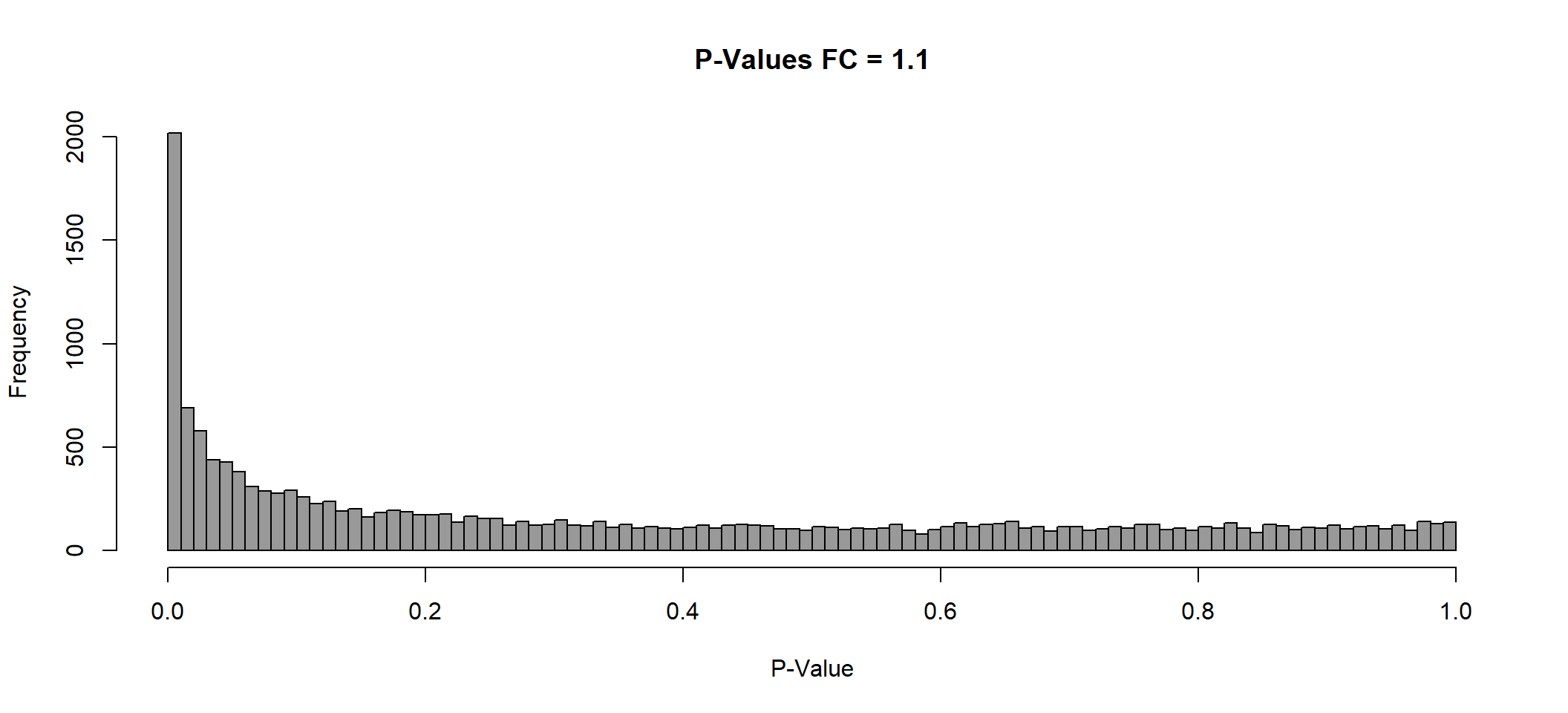
invisible(dev.print(svg, here::here(paste0("2_plots/de/pval_", fc[2], ".svg"))))MA Plot
ma[[2]]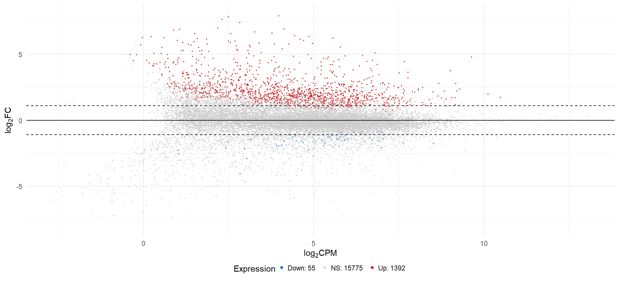
Volcano Plot
vol[[2]]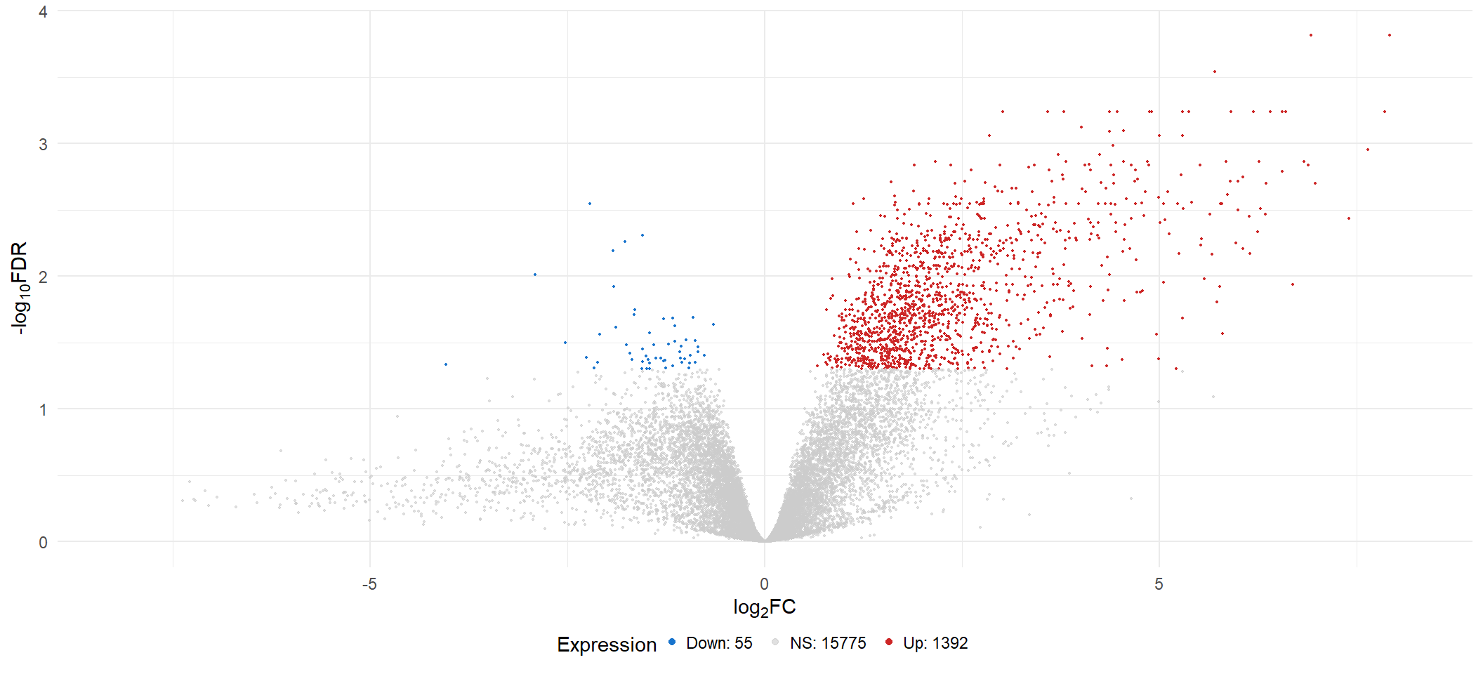
Top Upregulated
heat_up[[2]] 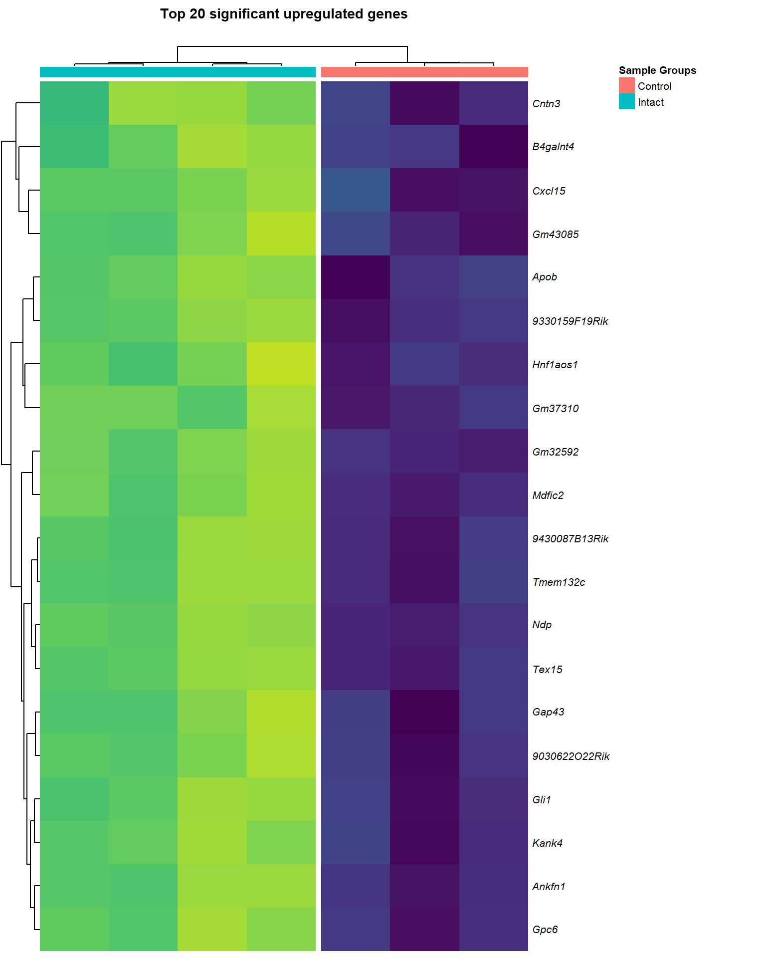
Top Downregulated
heat_down[[2]]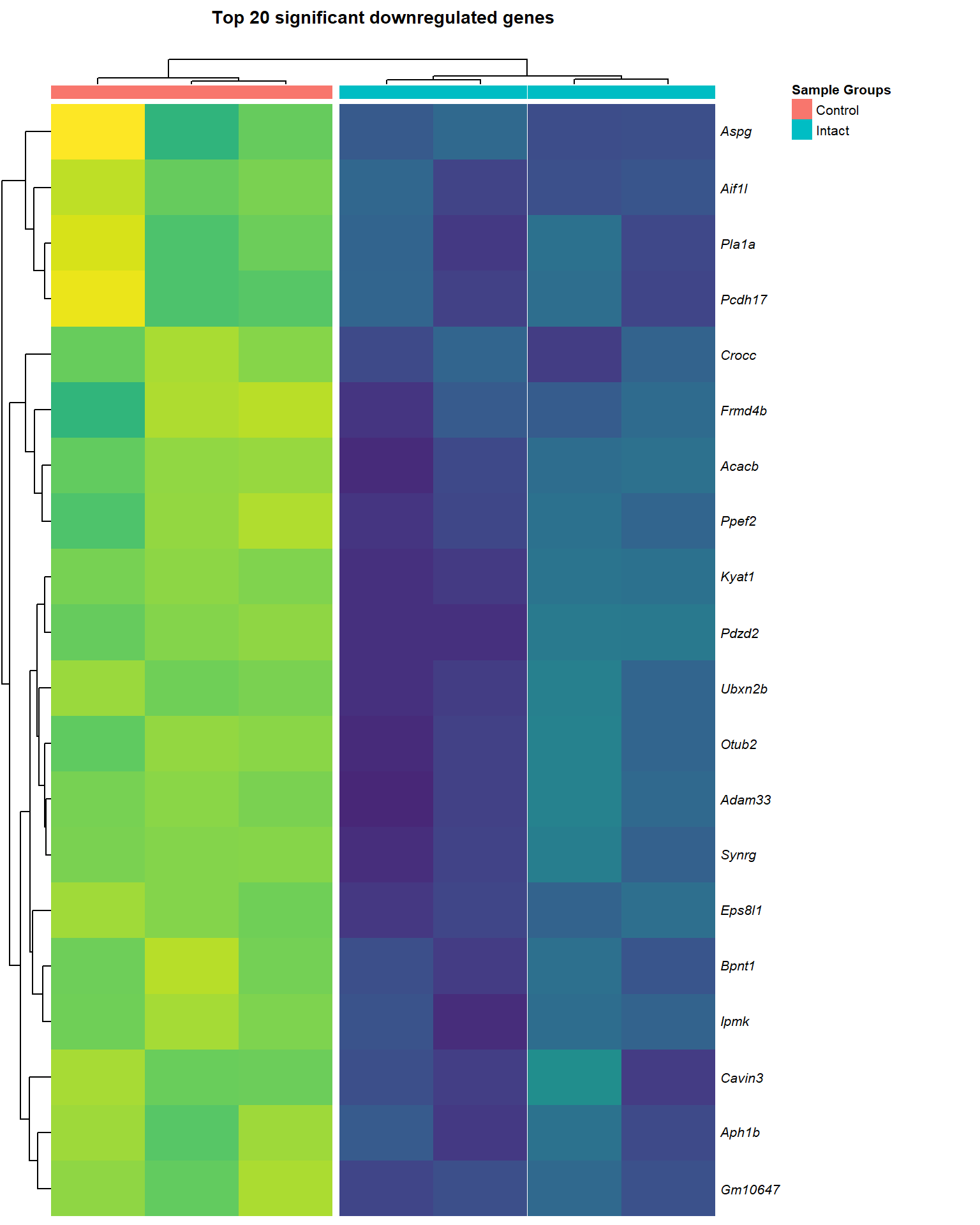
TREAT FC=1.5
assign(paste0("lmTreat_fc", fc[3], "_voom2_fdr0.05"),
limmaFit_treat(x = voom2, fc = fc[3], adjMethod = "fdr", p.val = 0.05))| INT vs CONT | |
|---|---|
| Down | 2 |
| NotSig | 16834 |
| Up | 386 |
assign(paste0("lmTreat_fc", fc[3], "_voom2_pval0.01"),
limmaFit_treat(x = voom2, fc = fc[3], adjMethod = "none", p.val = 0.01))| INT vs CONT | |
|---|---|
| Down | 14 |
| NotSig | 16238 |
| Up | 970 |
assign(paste0("lmTreat_fc", fc[3], "_voom2_pval0.05"),
limmaFit_treat(x = voom2, fc = fc[3], adjMethod = "none", p.val = 0.05))| INT vs CONT | |
|---|---|
| Down | 155 |
| NotSig | 15317 |
| Up | 1750 |
INT vs CONT Visualisation
P Value histogram
plot(x = lmTreat_hist[[3]],
     main = paste0("P-Values FC = ", fc[[3]]),
     xlab = "P-Value",
     col = "gray60")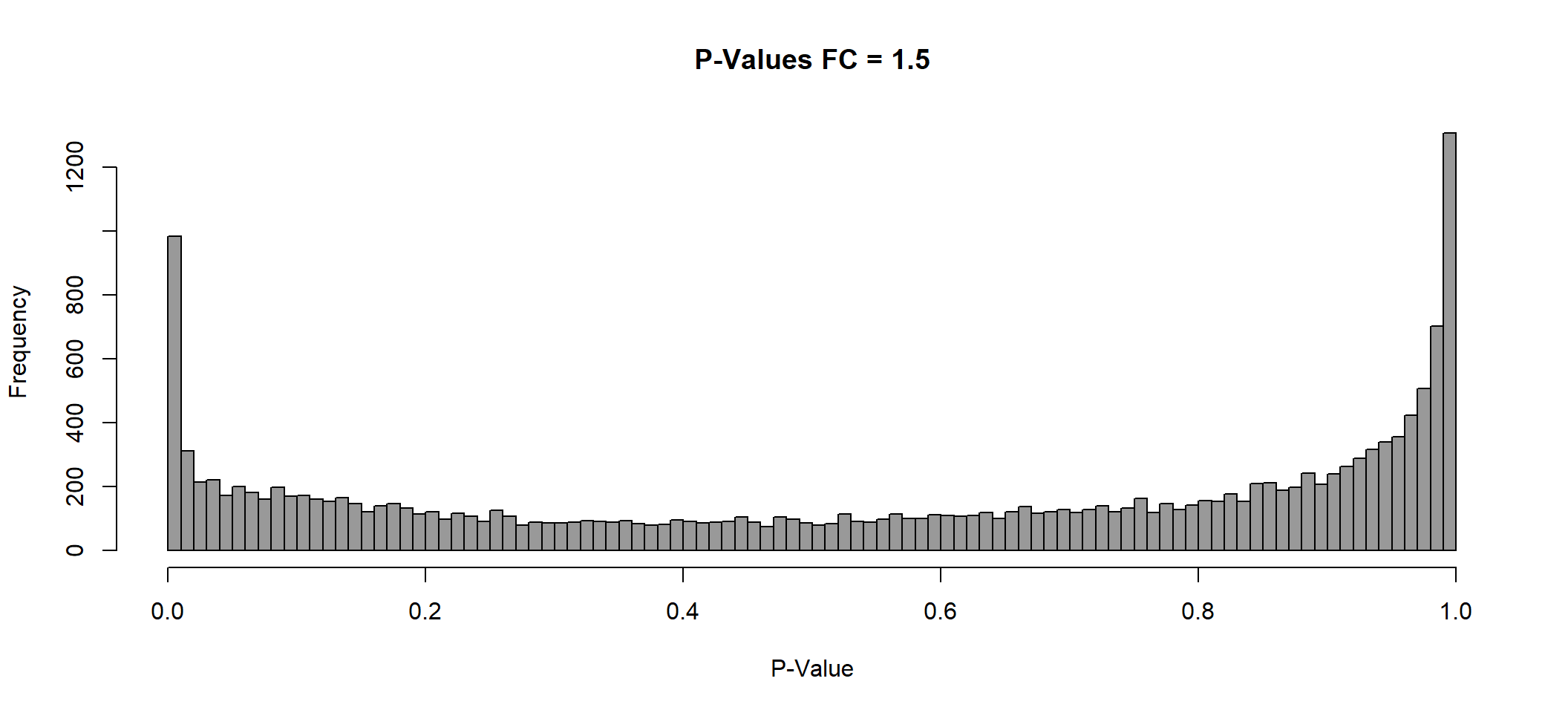
invisible(dev.print(svg, here::here(paste0("2_plots/de/pval_", fc[3], ".svg"))))MA Plot
ma[[3]]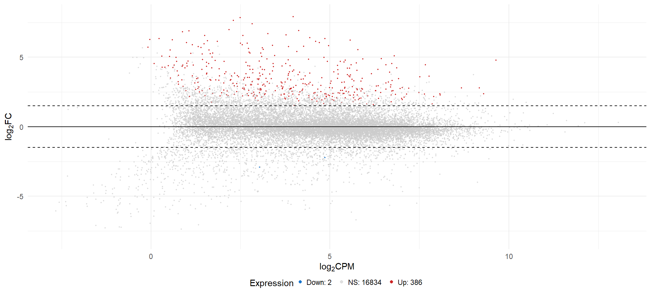
Volcano Plot
vol[[3]]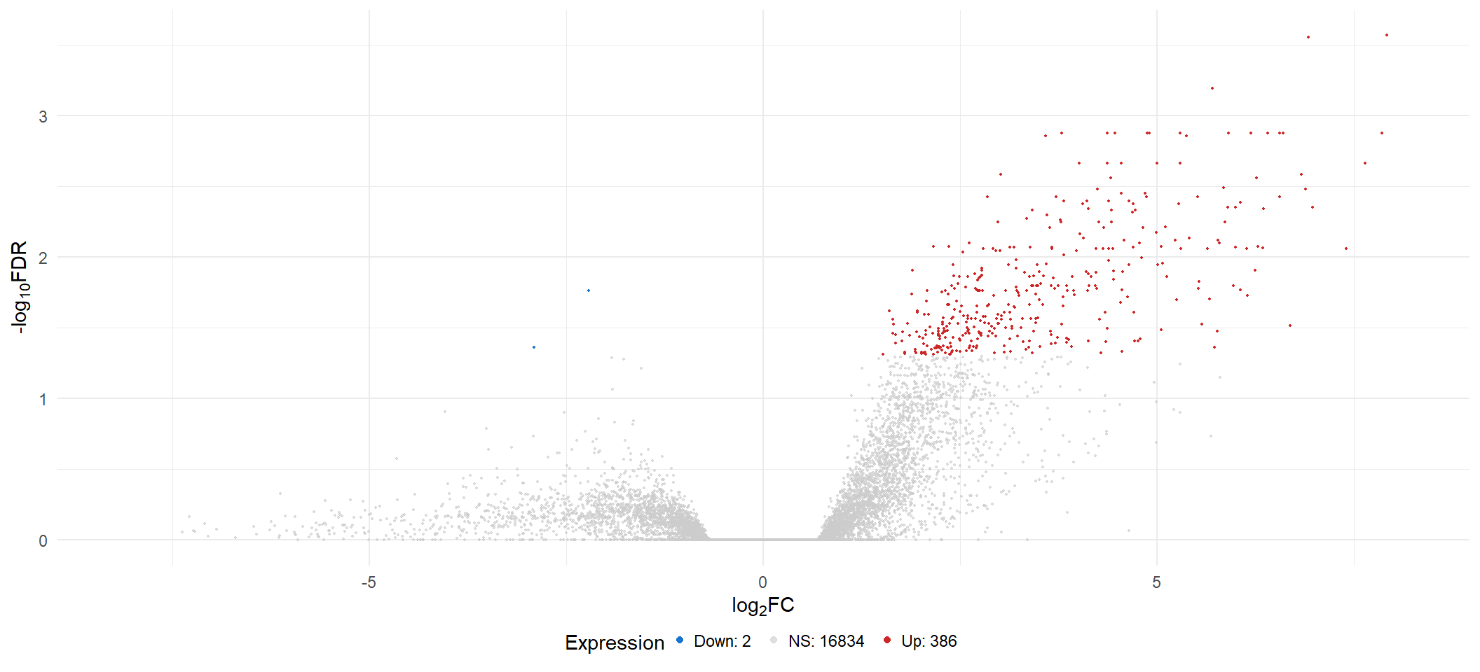
Top Upregulated
heat_up[[3]] 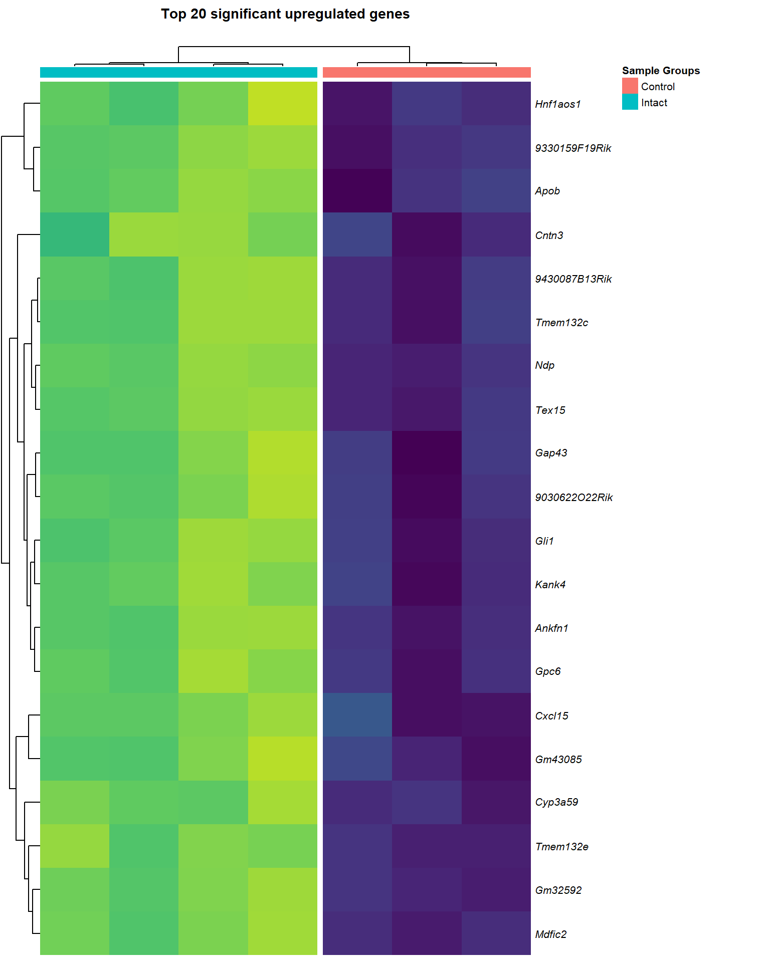
Top Downregulated
heat_down[[3]]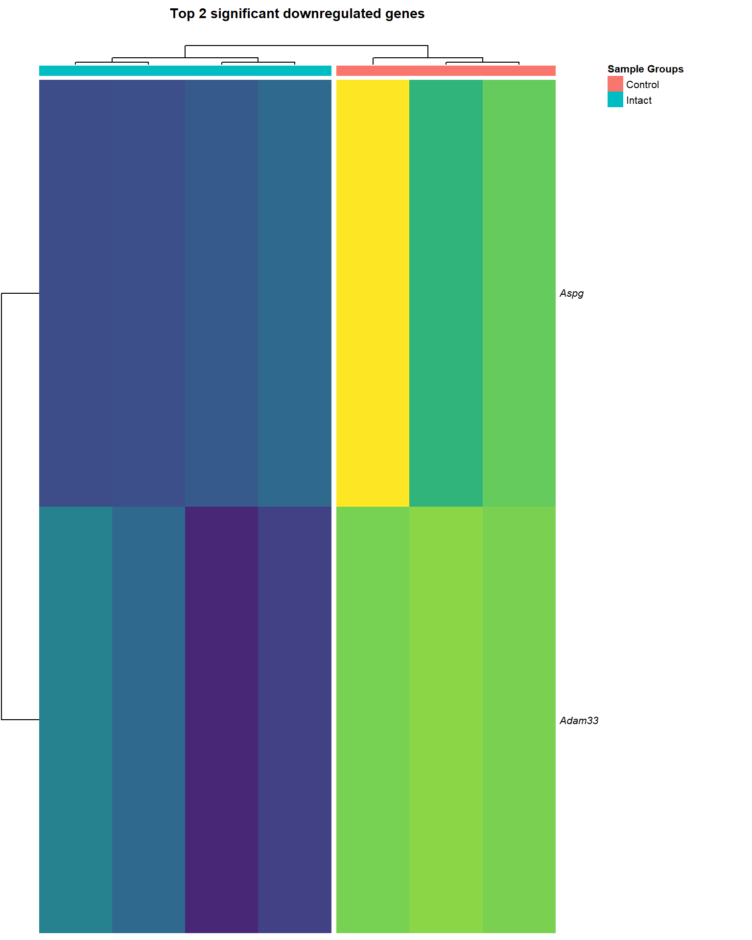
Export Data
# export toptable for Dexter rewrite
## First paper (suitable # of DE genes for INT vs CONT)
writexl::write_xlsx(x = lmTreat_fc1.5_voom2_fdr0.05, here::here("3_output/lmTreat_fc1.5_voom2_all_fdr.xlsx"))
## Second paper (suitable # of DE genes for INT vs SVS_VAS, SVX vs SVX_VAS, and VAS vs SVX_VAS)
writexl::write_xlsx(x = lm_voom2_pval0.01, here::here("3_output/lm_voom2_all.xlsx"))

# export excel spreadsheet
writexl::write_xlsx(x = lmTreat_all, here::here("3_output/lmTreat_all.xlsx"))
writexl::write_xlsx(x = lmTreat_sig, here::here("3_output/lmTreat_sig.xlsx"))

# save RDS object for enrichment analysis
saveRDS(object = fc, file = here::here("0_data/RDS_objects/fc.rds"))
saveRDS(object = lfc, file = here::here("0_data/RDS_objects/lfc.rds"))
saveRDS(object = full_design, file = here::here("0_data/RDS_objects/full_design.rds"))
saveRDS(object = contrast, file = here::here("0_data/RDS_objects/contrast.rds"))
saveRDS(object = lmTreat, file = here::here("0_data/RDS_objects/lmTreat.rds"))
saveRDS(object = lmTreat_all, file = here::here("0_data/RDS_objects/lmTreat_all.rds"))
saveRDS(object = lmTreat_sig, file = here::here("0_data/RDS_objects/lmTreat_sig.rds"))
sessionInfo()R version 4.2.1 (2022-06-23 ucrt)
Platform: x86_64-w64-mingw32/x64 (64-bit)
Running under: Windows 10 x64 (build 19045)
Matrix products: default
locale:
[1] LC_COLLATE=English_Australia.utf8 LC_CTYPE=English_Australia.utf8
[3] LC_MONETARY=English_Australia.utf8 LC_NUMERIC=C
[5] LC_TIME=English_Australia.utf8
attached base packages:
[1] grid stats graphics grDevices utils datasets methods
[8] base
other attached packages:
[1] Glimma_2.6.0 edgeR_3.38.4 limma_3.52.4 viridis_0.6.2
[5] viridisLite_0.4.1 ggrepel_0.9.1 ggpubr_0.4.0 ggplotify_0.1.0
[9] pheatmap_1.0.12 cowplot_1.1.1 pander_0.6.5 kableExtra_1.3.4
[13] forcats_0.5.2 stringr_1.4.1 purrr_0.3.5 tidyr_1.2.1
[17] ggplot2_3.3.6 tidyverse_1.3.2 reshape2_1.4.4 tibble_3.1.8
[21] readr_2.1.3 magrittr_2.0.3 dplyr_1.0.10
loaded via a namespace (and not attached):
[1] readxl_1.4.1 backports_1.4.1
[3] workflowr_1.7.0 systemfonts_1.0.4
[5] plyr_1.8.7 splines_4.2.1
[7] BiocParallel_1.30.3 GenomeInfoDb_1.32.4
[9] digest_0.6.29 yulab.utils_0.0.5
[11] htmltools_0.5.3 fansi_1.0.3
[13] memoise_2.0.1 googlesheets4_1.0.1
[15] tzdb_0.3.0 Biostrings_2.64.1
[17] annotate_1.74.0 modelr_0.1.9
[19] matrixStats_0.62.0 svglite_2.1.0
[21] colorspace_2.0-3 blob_1.2.3
[23] rvest_1.0.3 textshaping_0.3.6
[25] haven_2.5.1 xfun_0.33
[27] crayon_1.5.2 RCurl_1.98-1.9
[29] jsonlite_1.8.2 genefilter_1.78.0
[31] survival_3.3-1 glue_1.6.2
[33] gtable_0.3.1 gargle_1.2.1
[35] zlibbioc_1.42.0 XVector_0.36.0
[37] webshot_0.5.4 DelayedArray_0.22.0
[39] car_3.1-0 BiocGenerics_0.42.0
[41] abind_1.4-5 scales_1.2.1
[43] DBI_1.1.3 rstatix_0.7.0
[45] Rcpp_1.0.9 xtable_1.8-4
[47] gridGraphics_0.5-1 bit_4.0.4
[49] stats4_4.2.1 htmlwidgets_1.5.4
[51] httr_1.4.4 RColorBrewer_1.1-3
[53] ellipsis_0.3.2 farver_2.1.1
[55] pkgconfig_2.0.3 XML_3.99-0.11
[57] sass_0.4.2 dbplyr_2.2.1
[59] here_1.0.1 locfit_1.5-9.6
[61] utf8_1.2.2 labeling_0.4.2
[63] tidyselect_1.2.0 rlang_1.0.6
[65] later_1.3.0 AnnotationDbi_1.58.0
[67] munsell_0.5.0 cellranger_1.1.0
[69] tools_4.2.1 cachem_1.0.6
[71] cli_3.4.1 generics_0.1.3
[73] RSQLite_2.2.18 broom_1.0.1
[75] evaluate_0.17 fastmap_1.1.0
[77] ragg_1.2.3 yaml_2.3.5
[79] knitr_1.40 bit64_4.0.5
[81] fs_1.5.2 KEGGREST_1.36.3
[83] xml2_1.3.3 compiler_4.2.1
[85] rstudioapi_0.14 png_0.1-7
[87] ggsignif_0.6.3 reprex_2.0.2
[89] geneplotter_1.74.0 bslib_0.4.0
[91] stringi_1.7.8 highr_0.9
[93] lattice_0.20-45 Matrix_1.5-1
[95] vctrs_0.4.2 pillar_1.8.1
[97] lifecycle_1.0.3 jquerylib_0.1.4
[99] bitops_1.0-7 httpuv_1.6.6
[101] GenomicRanges_1.48.0 R6_2.5.1
[103] promises_1.2.0.1 gridExtra_2.3
[105] writexl_1.4.0 IRanges_2.30.1
[107] codetools_0.2-18 assertthat_0.2.1
[109] SummarizedExperiment_1.26.1 DESeq2_1.36.0
[111] rprojroot_2.0.3 withr_2.5.0
[113] S4Vectors_0.34.0 GenomeInfoDbData_1.2.8
[115] parallel_4.2.1 hms_1.1.2
[117] rmarkdown_2.17 MatrixGenerics_1.8.1
[119] carData_3.0-5 googledrive_2.0.0
[121] git2r_0.30.1 Biobase_2.56.0
[123] lubridate_1.8.0