Setting up for DGE analysis
Ha Tran
02/09/2021
Last updated: 2023-01-20
Checks: 6 1
Knit directory: SRB_2022/1_analysis/
This reproducible R Markdown analysis was created with workflowr (version 1.7.0). The Checks tab describes the reproducibility checks that were applied when the results were created. The Past versions tab lists the development history.
The R Markdown file has unstaged changes. To know which version of
the R Markdown file created these results, you’ll want to first commit
it to the Git repo. If you’re still working on the analysis, you can
ignore this warning. When you’re finished, you can run
wflow_publish to commit the R Markdown file and build the
HTML.
Great job! The global environment was empty. Objects defined in the global environment can affect the analysis in your R Markdown file in unknown ways. For reproduciblity it’s best to always run the code in an empty environment.
The command set.seed(12345) was run prior to running the
code in the R Markdown file. Setting a seed ensures that any results
that rely on randomness, e.g. subsampling or permutations, are
reproducible.
Great job! Recording the operating system, R version, and package versions is critical for reproducibility.
Nice! There were no cached chunks for this analysis, so you can be confident that you successfully produced the results during this run.
Great job! Using relative paths to the files within your workflowr project makes it easier to run your code on other machines.
Great! You are using Git for version control. Tracking code development and connecting the code version to the results is critical for reproducibility.
The results in this page were generated with repository version 6e0f643. See the Past versions tab to see a history of the changes made to the R Markdown and HTML files.
Note that you need to be careful to ensure that all relevant files for
the analysis have been committed to Git prior to generating the results
(you can use wflow_publish or
wflow_git_commit). workflowr only checks the R Markdown
file, but you know if there are other scripts or data files that it
depends on. Below is the status of the Git repository when the results
were generated:
Ignored files:
    Ignored:    .Rhistory
    Ignored:    .Rproj.user/

Untracked files:
    Untracked:  .gitignore
    Untracked:  test plz delete me.Rmd
    Untracked:  test-plz-delete-me.html

Unstaged changes:
    Modified:   0_data/RDS_objects/enrichGO_sig.rds
    Modified:   1_analysis/_site.yml
    Modified:   1_analysis/deAnalysis.Rmd
    Modified:   1_analysis/go.Rmd
    Modified:   1_analysis/index.Rmd
    Modified:   1_analysis/kegg.Rmd
    Modified:   1_analysis/reactome.Rmd
    Modified:   1_analysis/setUp.Rmd
    Modified:   2_plots/de/ma_1.05.png
    Modified:   2_plots/de/ma_1.1.png
    Modified:   2_plots/de/ma_1.5.png
    Modified:   2_plots/go/bp_dot_1.05.svg
    Modified:   2_plots/go/bp_dot_1.1.svg
    Modified:   2_plots/go/bp_dot_1.5.svg
    Modified:   2_plots/go/cc_dot_1.05.svg
    Modified:   2_plots/go/cc_dot_1.1.svg
    Modified:   2_plots/go/cc_dot_1.5.svg
    Modified:   2_plots/go/mf_dot_1.05.svg
    Modified:   2_plots/go/mf_dot_1.1.svg
    Modified:   2_plots/go/mf_dot_1.5.svg
    Deleted:    2_plots/ipa/funct_cat_alluvial.svg
    Deleted:    2_plots/ipa/up_cat_alluvial.svg
    Deleted:    2_plots/ipa/upstream_funct_alluvial.svg
    Modified:   2_plots/kegg/kegg_dot_1.05.svg
    Modified:   2_plots/kegg/kegg_dot_1.1.svg
    Modified:   2_plots/kegg/kegg_dot_1.5.svg
    Deleted:    2_plots/reactome/combine_GO.svg
    Modified:   2_plots/reactome/react_dot_1.05.svg
    Modified:   2_plots/reactome/react_dot_1.1.svg
    Modified:   2_plots/reactome/react_dot_1.5.svg
    Deleted:    2_plots/reactome/react_dot_INT vs CONT.svg
    Deleted:    2_plots/reactome/react_dot_INT vs SVX_VAS.svg
    Deleted:    2_plots/reactome/react_dot_SVX vs SVX_VAS.svg
    Deleted:    2_plots/reactome/react_dot_VAS vs SVX_VAS.svg
    Deleted:    2_plots/reactome/upset_react_INT vs CONT.svg
    Deleted:    2_plots/reactome/upset_react_INT vs SVX_VAS.svg
    Deleted:    2_plots/reactome/upset_react_SVX vs SVX_VAS.svg
    Deleted:    2_plots/reactome/upset_react_VAS vs SVX_VAS.svg
    Modified:   3_output/enrichGO_sig.xlsx
    Modified:   3_output/enrichKEGG_all.xlsx
    Modified:   3_output/enrichKEGG_sig.xlsx
    Modified:   3_output/lmTreat_all.xlsx
    Modified:   3_output/lmTreat_fc1.5_voom2_all_fdr.xlsx
    Modified:   3_output/lmTreat_sig.xlsx
    Modified:   3_output/reactome_all.xlsx
    Modified:   3_output/reactome_sig.xlsx
Note that any generated files, e.g. HTML, png, CSS, etc., are not included in this status report because it is ok for generated content to have uncommitted changes.
These are the previous versions of the repository in which changes were
made to the R Markdown (1_analysis/setUp.Rmd) and HTML
(docs/setUp.html) files. If you’ve configured a remote Git
repository (see ?wflow_git_remote), click on the hyperlinks
in the table below to view the files as they were in that past version.
| File | Version | Author | Date | Message |
|---|---|---|---|---|
| html | 691cf34 | Ha Manh Tran | 2023-01-20 | Build site. |
| Rmd | 7f6bab2 | Ha Manh Tran | 2023-01-20 | workflowr::wflow_publish(here::here("1_analysis/*.Rmd")) |
| Rmd | b6cf190 | tranmanhha135 | 2023-01-19 | quick commit |
| Rmd | 3119fad | tranmanhha135 | 2022-11-05 | build website |
| html | 3119fad | tranmanhha135 | 2022-11-05 | build website |
Data Setup
Prior to this analysis, reads were: 1. Trimmed using
AdapterRemoval 2. Aligned to GRCm38/mm10
using STAR 3. Reads quantification performed with
featureCounts
Transcript QC, alignment, and quantification were performed by Dr Jimmy Breen
# working with data
library(dplyr)
library(magrittr)
library(readr)
library(tibble)
library(reshape2)
library(tidyverse)
library(bookdown)

# Visualisation:
library(kableExtra)
library(ggbiplot)
library(ggrepel)
library(grid)
library(cowplot)
library(corrplot)

# Set ggplot theme
theme_set(theme_light())

pub <- theme_update(
  plot.title = element_text(color = "gray20", size = 12, angle = 0, hjust = 0.5, vjust = .5, face = "bold"),
  plot.subtitle = element_text(color = "gray20", size = 11, angle = 0, hjust = 0, vjust = .5, face = "plain"),
  legend.title = element_text(color = "gray20", size = 11, angle = 0, hjust = 0.5, vjust = .5, face = "plain"),
  legend.text = element_text(color = "gray20", size = 11, angle = 0, hjust = 0, vjust = .5, face = "plain"),
  axis.text.x = element_text(color = "gray20", size = 11, angle = 0, hjust = .5, vjust = 0, face = "plain"),
  axis.title.x = element_text(color = "gray20", size = 11, angle = 0, hjust = .5, vjust = 0, face = "plain"),
  axis.text.y = element_text(color = "gray20", size = 11, angle = 0, hjust = 1, vjust = 0.5, face = "plain"),
  axis.title.y = element_text(color = "gray20", size = 11, angle = 90, hjust = .5, vjust = .5, face = "plain"))

# Bioconductor packages:
library(AnnotationHub)
library(edgeR)
library(limma)
library(Glimma)
Import Raw Count Data
Due to the unusual library size, control 3 was removed from the analysis
# import the mergedOnly dataset, provided by Dr Jimmy Breen on the 24/09/21
rawCount <- read_tsv(here::here("0_data/raw_data/allSamples_mergedOnly.featureCounts.txt"),
                     col_names = TRUE,
                     comment = "#") %>%
  dplyr::rename(CONT1 = "../2_Hisat2_merged/CONT1_ATGTCA_merged.sorted.nodup.bam",
                CONT2 = "../2_Hisat2_merged/CONT2_CGATGT_merged.sorted.nodup.bam",
                CONT4 = "../2_Hisat2_merged/CONT4_ACTTGA_merged.sorted.nodup.bam",
                INT1 = "../2_Hisat2_merged/INT1_GTCCGC_merged.sorted.nodup.bam",
                INT2 = "../2_Hisat2_merged/INT2_ACAGTG_merged.sorted.nodup.bam",
                INT3 = "../2_Hisat2_merged/INT3_GATCAG_merged.sorted.nodup.bam",
                INT4 = "../2_Hisat2_merged/INT4_CTTGTA_merged.sorted.nodup.bam",
                SVX1 = "../2_Hisat2_merged/SVX1_GTTTCG_merged.sorted.nodup.bam",
                SVX2 = "../2_Hisat2_merged/SVX2_TAGCTT_merged.sorted.nodup.bam",
                SVX3 = "../2_Hisat2_merged/SVX3_ATCACG_merged.sorted.nodup.bam",
                SVX4 = "../2_Hisat2_merged/SVX4_GCCAAT_merged.sorted.nodup.bam",
                SVX_VAS1 = "../2_Hisat2_merged/SVX_VAS1_AGTCAA_merged.sorted.nodup.bam",
                SVX_VAS2 = "../2_Hisat2_merged/SVX_VAS2_AGTTCC_merged.sorted.nodup.bam",
                SVX_VAS3 = "../2_Hisat2_merged/SVX_VAS3_TGACCA_merged.sorted.nodup.bam",
                SVX_VAS4 = "../2_Hisat2_merged/SVX_VAS4_GGCTAC_merged.sorted.nodup.bam",
                VAS1 = "../2_Hisat2_merged/VAS1_CAGATC_merged.sorted.nodup.bam",
                VAS2 = "../2_Hisat2_merged/VAS2_GTGAAA_merged.sorted.nodup.bam",
                VAS3 = "../2_Hisat2_merged/VAS3_GTGGCC_merged.sorted.nodup.bam",
                VAS4 = "../2_Hisat2_merged/VAS4_CCGTCC_merged.sorted.nodup.bam",) %>%
  column_to_rownames("Geneid") %>%
  as.data.frame()
  rownames(rawCount) <- gsub("\\..+$", "", rownames(rawCount))

# Removing the non-numerical metadata column. SVX_VAS1 may also be an outlier, it is number 18 (BTW)
rawCount<- rawCount[, c(6,7,9:25)]
Import Metadata
There are generally two metadata required for DGE analysis.
metadata about each sample
metadata about each gene
Sample Metadata
The sample metadata can be extracted from the logCPM
column names. These data include sample_id,
sample_group, sample_type.
The sample metadata will be manually generated and stored in the
/0_data/raw_data/ directory
samples <- read_tsv(here::here("0_data/raw_data/samples.tsv"),
                    col_names = TRUE) %>%
  column_to_rownames("1")
Gene Metadata
Gene annotation is useful for the DGE analysis as it will provide useful information about the genes. The annotated genes of Mus musculus can be pulled down by using Annotation Hub.
Annotation Hub also has a web service that can be assessed through
the display function. Pulling down the gene annotation can take a long
time, so after the initial run, the annotated genes is saved to a
genes.rds file. To save time, if genes.rds is
already present, don’t run the code chunk.
ah <- AnnotationHub()
ah %>%
  subset(grepl("musculus", species)) %>%
  subset(rdataclass == "EnsDb")

#viewing web service for annotation hub
#d <- display(ah)

# Annotation hub html site was used to identify 'code' for the latest mouse genome from Ensembl
ensDb <- ah[["AH95775"]]

genes <- genes(ensDb) %>%
  as.data.frame()

#the annotated genes are saved into a RDS object to save computational time in subsequent run of the setUp.Rmd
genes %>% saveRDS(here::here("0_data/RDS_objects/gene_metadata.rds"))
Using the annotated gene list through AnnotationHub(), load into
object called geneMetadata. Filter out all genes that are
present in the rawCount and display the number of unique gene_biotypes
present in the rawCount and geneMetadata
geneMetadata <- read_rds(here::here("0_data/RDS_objects/gene_metadata.rds"))

#prepare the gene data frame to contain the genes listed in the rownames of 'rawCount' data
geneMetadata <- data.frame(gene = rownames(rawCount)) %>%
  left_join(geneMetadata %>% as.data.frame,
            by = c("gene"="gene_id")) %>%
  dplyr::distinct(gene, .keep_all=TRUE)

rownames(geneMetadata) <- geneMetadata$gene

#Using the table function, the details of the genes present in the rawCount data can be summaried.
genes <- geneMetadata$gene_biotype %>% table %>% as.data.frame()

colnames(genes) <- c("Gene Biotype", "Frequency")

kable(genes) %>% kable_styling(bootstrap_options = c("striped", "hover")) %>% scroll_box(height = "600px")| Gene Biotype | Frequency |
|---|---|
| IG_C_gene | 13 |
| IG_C_pseudogene | 1 |
| IG_D_gene | 19 |
| IG_D_pseudogene | 4 |
| IG_J_gene | 14 |
| IG_LV_gene | 4 |
| IG_pseudogene | 1 |
| IG_V_gene | 218 |
| IG_V_pseudogene | 155 |
| lncRNA | 7128 |
| miRNA | 1124 |
| misc_RNA | 32 |
| Mt_rRNA | 2 |
| Mt_tRNA | 22 |
| polymorphic_pseudogene | 76 |
| processed_pseudogene | 7047 |
| protein_coding | 21575 |
| pseudogene | 59 |
| ribozyme | 20 |
| rRNA | 13 |
| scaRNA | 34 |
| scRNA | 1 |
| snoRNA | 1065 |
| snRNA | 789 |
| TEC | 2587 |
| TR_C_gene | 8 |
| TR_D_gene | 4 |
| TR_J_gene | 70 |
| TR_J_pseudogene | 10 |
| TR_V_gene | 144 |
| TR_V_pseudogene | 34 |
| transcribed_processed_pseudogene | 214 |
| transcribed_unitary_pseudogene | 21 |
| transcribed_unprocessed_pseudogene | 223 |
| translated_unprocessed_pseudogene | 2 |
| unitary_pseudogene | 13 |
| unprocessed_pseudogene | 2310 |
Create DGEList object
Digital Gene Expression List (DGElist) is a R object class often used for differential gene expression analysis as it simplifies plotting, and interaction with data and metadata.
The DGEList object holds the three dataset that have
imported/created, including rawCount data and
sampleMetadata and geneMetadata metadata.
To further save time and memory, genes that were not expressed across
all samples (i.e., 0 count across all columns) are all
removed
#Create DGElist with rawCOunt and gene data. Remove all genes with 0 expression in all treatment groups
dge <- DGEList(counts = rawCount,
               samples = samples,
               genes = geneMetadata,
               remove.zeros = TRUE
               )
Pre-processing and QC
Pre-processing steps increased the power of the downstream DGE analysis by eliminating majority of unwanted variance that could obscure the true variance caused by the differences in sample conditions. There are several standard steps that are commonly followed to pre-process and QC raw read counts, including:
Checking Library Size
Removal of Undetectable Genes
Normalisation
QC through MDS/PCA
Checking Library Size
A simple pre-processing/QC step is checking the quality of library
size (total number of mapped and quantified reads) for each treatment.
This enable identification of potentially mis-labelled or outlying
samples. This is often visualised through ggplot.
libSize <- dge$samples %>%

  #plot the sample with the lib.size in x and sample_group in y, colour fill for each sample_group
  ggplot(aes(
    x = lib.size,
    y = rownames(dge$samples),
    fill = dge$samples$group)
    ) +
  geom_col() +

  #draw a vertical line for the mean lib.size
  geom_vline(
    aes (xintercept = lib.size),
    data = . %>% summarise_at(vars(lib.size), mean),
    linetype = 2
  ) +

  #labelling splot
  labs(
    title = "Sample Library Size",
    x = "Library Size",
    y = "Samples",
    fill = "Sample Groups"
  ) +

  #PUBLISHING
  theme(legend.position = "none")

libSize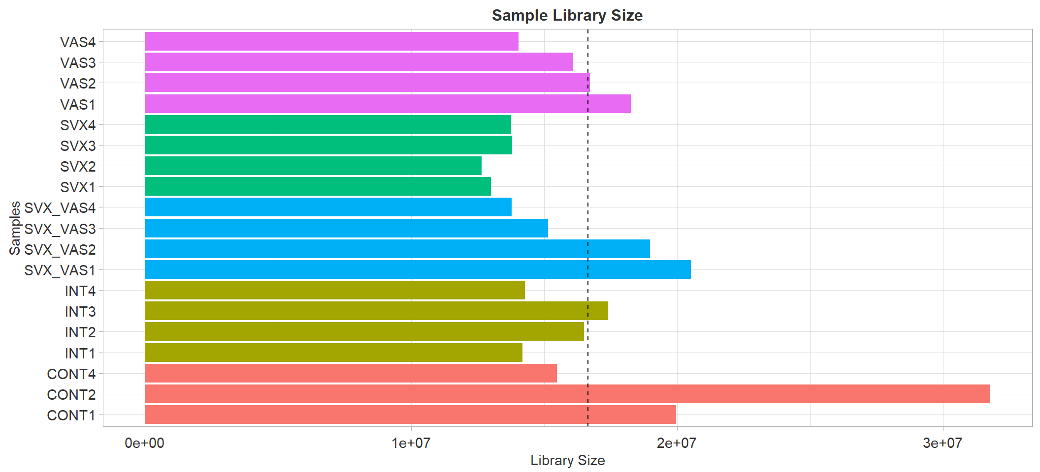
Sample library size. Dash line represent average library size
#save the plot to .svg
ggsave(here::here("2_plots/qc/library_size.svg"),
       plot = libSize + pub,
       #PUBLISHING
       width = 250,
       height = 166,
       units = "mm")
Removal of Low-Expressed Genes
Filtering out low-expressed genes is a standard pre-processing step in DGE analysis as it can significantly increase the power to differentiate differentially expressed genes by eliminating the variance caused by genes that are lowly expressed in all samples.
The threshold of removal is arbitrary and is often determined after
visualisation of the count distribution. The count distribution can be
illustrated in a density plot through ggplot. A common
metric used to display the count distribution is log Counts per
Million (logCPM)
beforeFiltering <- dge %>%

  #transform the raw count to logCPM
  edgeR::cpm(log = TRUE) %>%

  #melting (reorganising) the transformed logCPM data with respect to the id variable (i.e., the row and column names). Very similar to pivot_long function
  melt %>%

  #retain all rows where the logCPM (value) is finite. All of them in this case are finite
  dplyr::filter(is.finite(value)) %>%

  #plot the long formate logCPM counts in a density plot with x the logCPM and colour by the sample_id
  ggplot(aes(
    x = value,
    colour = Var2
  )) +
  geom_density() +

  # remove the legend
  guides(colour = FALSE) +

  #add figure tittle and subtitle and labels
  ggtitle("Before Filtering Low-expressed Genes", subtitle = paste0(nrow(dge), " genes"))+
  labs(
    x = "logCPM",
    y = "Density",
    colour = "Sample Groups"
  )

#save plot
ggsave("counts_before_filtering.svg",
       plot = beforeFiltering + pub,
       width = 250,
       height = 166,
       units = "mm",
       path = here::here("2_plots/qc/"))
Ideally, the filtering the low-expressed genes should remove the
large peak with logCPM < 0, i.e., remove any genes which
have less than one count per million.
A common guideline is to keep all genes that have > 1-2 cpm in the
smallest group on a treatment. In this case, the smallest group is 3 as
each treatment condition had three replicates. However, due to the high
variance of some groups, the filtering is increased to keep genes that
are are more than 3 CPM in at least 3 samples.
Mathematically this would be identifying genes (rows) with CPM
> 3; and identifying total row sum that is
>= 3.
#the genes kept have >2 CPM for at least 3 samples
keptGenes <- (rowSums(cpm(dge) > 3) >= 3)
afterFiltering <- dge %>%

  #transform the raw count to logCPM
  edgeR::cpm(log = TRUE) %>%

  #for var1 (gene names) extract only the keptGenes and discard all other genes in the logCPM data
  magrittr::extract(keptGenes,) %>%

  #melting (reorganising) the transformed logCPM data with respect to the id variable (i.e., the row and column names). Very similar to pivot_long function
  melt %>%

  #retain all rows where the logCPM (value) is finite. All of them in this case are finite
  dplyr::filter(is.finite(value)) %>%

  #ggplot
  ggplot(aes(
    x = value,
    colour = Var2
  )) +
  geom_density() +

  #remove the legend
  guides(colour = FALSE) +

  #add figure tittle and subtitle and labels. since keptGenes is a logic element, the second element represents the number of genes that were kept after the filtering
  ggtitle("After Filtering Low-expressed Genes", subtitle = paste0(table(keptGenes)[[2]], " genes")) +
  labs(
    x = "logCPM",
    y = "Density",
    colour = "Sample Groups"
  )

#save plot
ggsave("counts_after_filtering_3_3.svg",
       plot = afterFiltering + pub,
       width = 250,
       height = 166,
       units = "mm",
       path = here::here("2_plots/qc/"))

#display plot
# afterFiltering

#display plot side by side
cowplot::plot_grid(beforeFiltering + pub, afterFiltering + pub)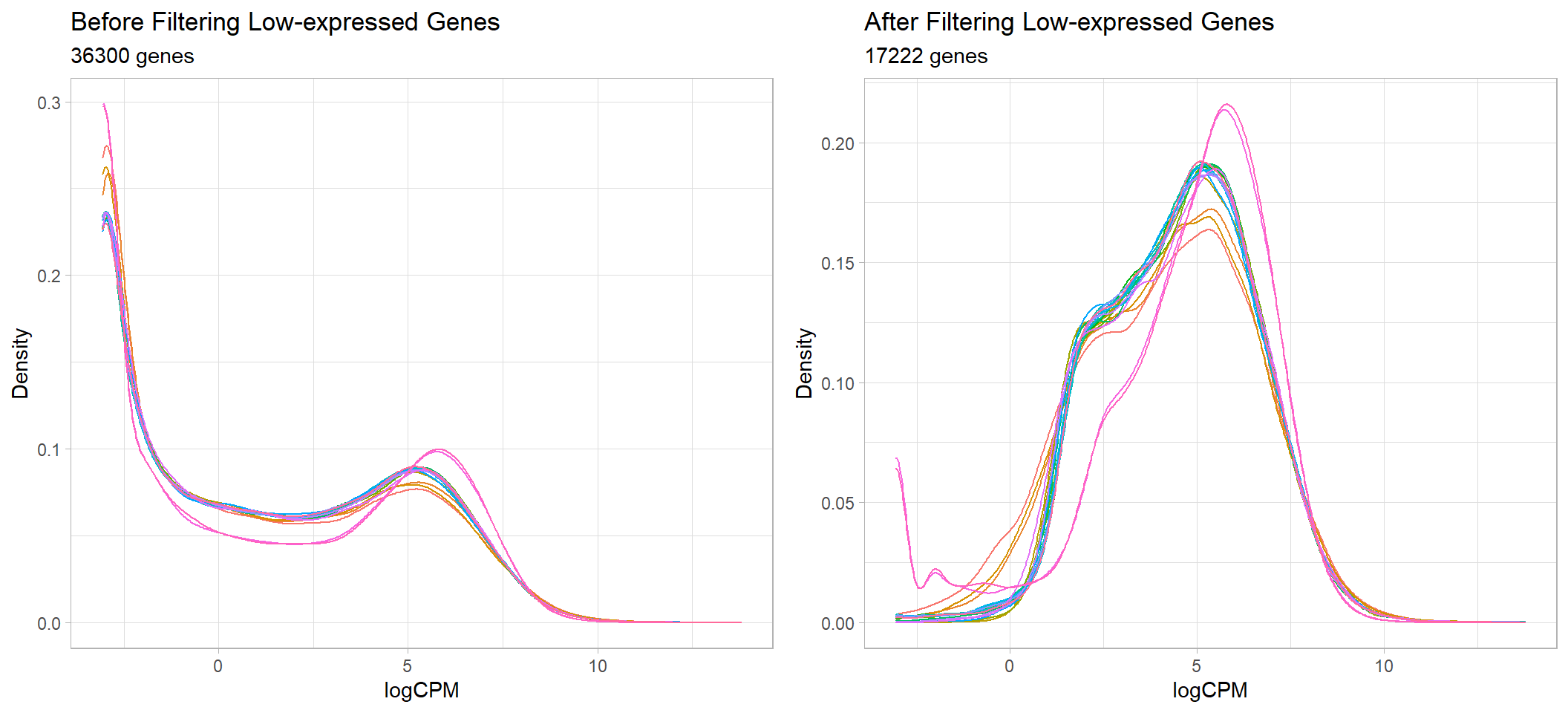
Before and after removal of lowly expressed genes
ggsave(filename = "counts_before_after_filtering_3_3.svg",
        path = here::here("2_plots/qc/"),

       # PUBLISHING
       width = 320,
       height = 180,
       units = "mm")
Following the filtering of low-expressed genes < 3 CPM in at least 3 samples, out of the total 36300 genes left after the removal of genes with no expression, 19078 genes were removed, leaving only 17222 genes remaining for the downstream analysis
Subset the DGElist object
After filtering the low-expressed genes, the DGElist object is updated to eliminate the low-expressed genes from future analysis
#extract genes from keptGenes and recalculate the lib size
dge <- dge[keptGenes,,keep.lib.sizes = FALSE]
Normalisation
Using the TMM (trimmed mean of M value) method of normalisation
through the edgeR package. The TMM approach creates a
scaling factor as an offset to be supplied to Negative Binomial model.
The ca;cNormFactors function calculate the normalisation
and return the adjusted norm.factor to the
dge$samples element.
#after normalisation
dge <- edgeR::calcNormFactors(object = dge,
                              method = "TMM")
knitr::kable(dge$samples, caption = "Normalised samples") %>%
  kable_styling(bootstrap_options = c("striped", "hover")) %>%
scroll_box(height = "600px")| group | lib.size | norm.factors | sample | Mated | rep | pretty | |
|---|---|---|---|---|---|---|---|
| CONT1 | CONT | 19872706 | 0.8464567 | CONT1 | 0 | 1 | Control 1 |
| CONT2 | CONT | 31605394 | 0.8813685 | CONT2 | 0 | 2 | Control 2 |
| CONT4 | CONT | 15405575 | 0.8561445 | CONT4 | 0 | 4 | Control 4 |
| INT1 | INT | 14113774 | 0.9367904 | INT1 | 1 | 1 | Intact 1 |
| INT2 | INT | 16402891 | 0.9673697 | INT2 | 1 | 2 | Intact 2 |
| INT3 | INT | 17305033 | 1.0131402 | INT3 | 1 | 3 | Intact 3 |
| INT4 | INT | 14186233 | 1.0068550 | INT4 | 1 | 4 | Intact 4 |
| SVX1 | SVX | 12929360 | 0.9930892 | SVX1 | 1 | 1 | SVX 1 |
| SVX2 | SVX | 12576540 | 1.0110654 | SVX2 | 1 | 2 | SVX 2 |
| SVX3 | SVX | 13706572 | 0.9975451 | SVX3 | 1 | 3 | SVX 3 |
| SVX4 | SVX | 13679685 | 1.0203208 | SVX4 | 1 | 4 | SVX 4 |
| SVX_VAS1 | SVX_VAS | 20391320 | 1.0153981 | SVX_VAS1 | 1 | 1 | SVX-VAS 1 |
| SVX_VAS2 | SVX_VAS | 18854522 | 0.9565130 | SVX_VAS2 | 1 | 2 | SVX-VAS 2 |
| SVX_VAS3 | SVX_VAS | 15046800 | 1.0081015 | SVX_VAS3 | 1 | 3 | SVX-VAS 3 |
| SVX_VAS4 | SVX_VAS | 13703601 | 0.9920736 | SVX_VAS4 | 1 | 4 | SVX-VAS 4 |
| VAS1 | VAS | 18149990 | 0.9774237 | VAS1 | 1 | 1 | VAS 1 |
| VAS2 | VAS | 16595337 | 1.2915788 | VAS2 | 1 | 2 | VAS 2 |
| VAS3 | VAS | 15982473 | 1.3304675 | VAS3 | 1 | 3 | VAS 3 |
| VAS4 | VAS | 13942997 | 1.0157786 | VAS4 | 1 | 4 | VAS 4 |
Visualisation of TMM Normalisation
The following visualisation of the TMM normalisation is plotted using
the mean-difference (MD) plot. The MD plot visualise the library
size-adjusted logFC between two samples (the difference) against the
log-expression across all samples (the mean). In this instance,
sample 1 is used to compare against an artificial library
construct from the average of all the other samples
limma::plotMD(cpm(dge, log = TRUE), column=1)
abline(h=0, col="red", lty=2, lwd=2)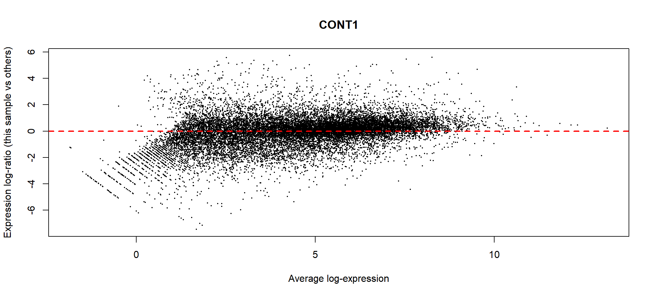
MA plot of TMM normalisation for control 1
Ideally, the bulk of gene expression following the TMM normalisation
should be centred around expression log-ratio of 0, which
indicates that library size bias between samples have been successfully
removed. This should be repeated with all the samples in the dge
object.
Quality Control
Pinciple Component Analysis (PCA)
samples <- dge$samples %>% rownames_to_column("sampleName")
samples$rep <- samples$rep %>% as.factor()


# Perform PCA analysis:
pca_analysis <- prcomp(t(cpm(dge, log = TRUE)))

summary(pca_analysis)$importance %>% as.data.frame()
group.colours <- c(CONT = "#F8766D", INT = "#A3A500")
# Create the plot
a <- pca_analysis$x %>%
as.data.frame() %>%
rownames_to_column("sampleName") %>%
left_join(samples) %>%
as_tibble() %>%
ggplot(aes(x = PC1, y = PC2, colour = group, shape = rep)) +
geom_point(size=3, alpha=0.5) +
scale_shape_manual(values = c(15:18)) +
labs(
x = paste0("PC1 (", percent(summary(pca_analysis)$importance["Proportion of Variance","PC1"]),")"),
y = paste0("PC2 (", percent(summary(pca_analysis)$importance["Proportion of Variance","PC2"]),")"),
colour = "Groups",
shape = "Replicates"
)
b <- pca_analysis$x %>%
as.data.frame() %>%
rownames_to_column("sampleName") %>%
left_join(samples) %>%
as_tibble() %>%
ggplot(aes(x = PC2, y = PC3, colour = group, shape = rep)) +
geom_point(size=3, alpha=0.5) +
scale_shape_manual(values = c(15:18)) +
labs(
x = paste0("PC2 (", percent(summary(pca_analysis)$importance["Proportion of Variance","PC2"]),")"),
y = paste0("PC3 (", percent(summary(pca_analysis)$importance["Proportion of Variance","PC3"]),")"),
colour = "Groups",
shape = "Replicates"
)
c <- pca_analysis$x %>%
as.data.frame() %>%
rownames_to_column("sampleName") %>%
left_join(samples) %>%
as_tibble() %>%
dplyr::slice(1:7) %>%
ggplot(aes(x = PC1, y = PC2, colour = group, shape = rep)) +
geom_point(size=3, alpha=0.8) +
scale_color_manual(values = group.colours)+
scale_shape_manual(values = c(15:18)) +
labs(
x = paste0("PC1 (", percent(summary(pca_analysis)$importance["Proportion of Variance","PC1"]),")"),
y = paste0("PC2 (", percent(summary(pca_analysis)$importance["Proportion of Variance","PC2"]),")"),
colour = "Groups",
shape = "Replicates"
)
c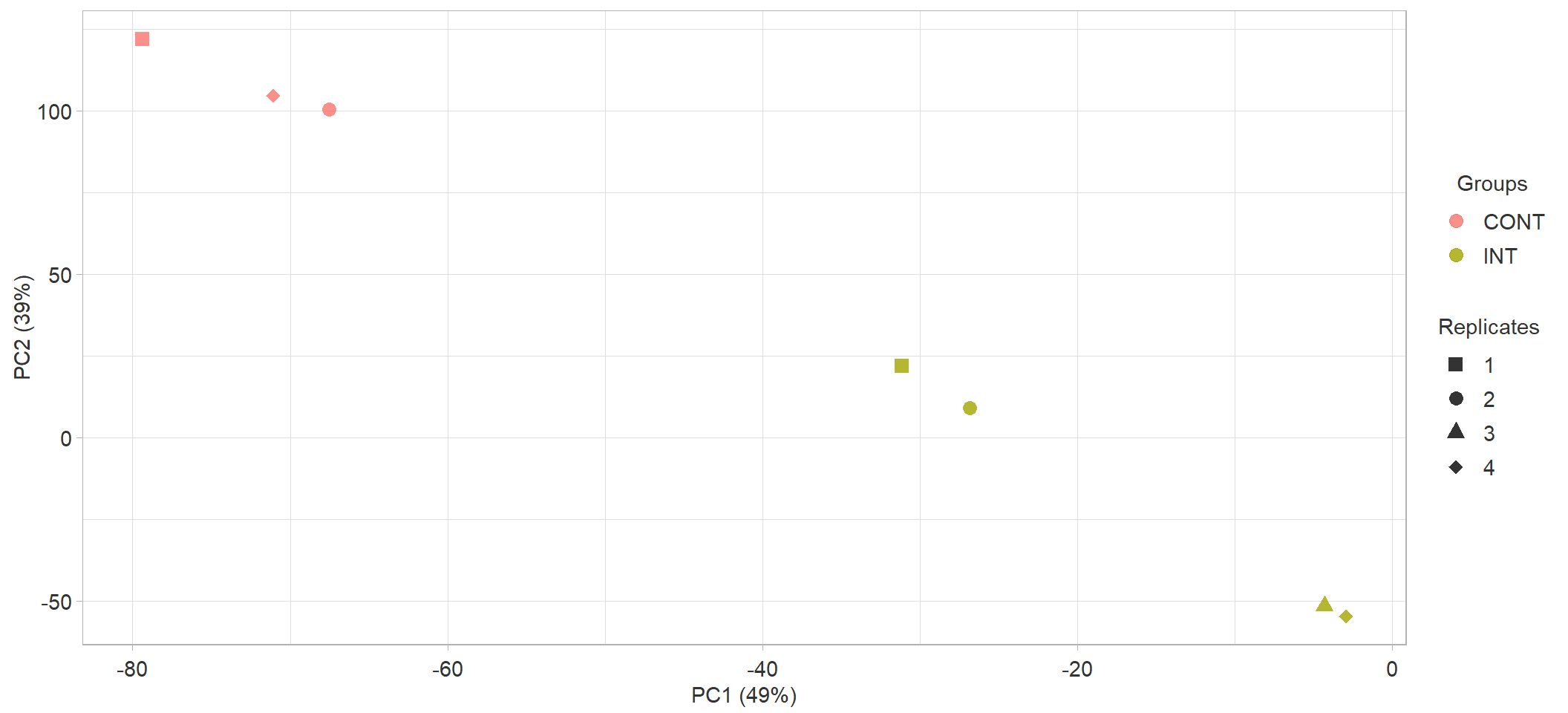
PCA plot of all samples.
ggsave("PCA_IntvsCont.svg",
       plot = c + pub,
       path = here::here("2_plots/qc/"),
       width = 150,
       height = 100,
       units = "mm")

# pca_plot_2 <- plot_grid(
#     plot_grid(
#         a + theme(legend.position = "none"),
#         b + theme(legend.position = "none"),
#         c + theme(legend.position = "none"),
#         nrow = 1
#     ),
#     get_legend(a + theme(legend.position = "bottom")),
#     nrow = 2,
#     rel_heights = c(4,1)
# )
#
#
# pca_plot_2


# ggsave("PCA_plot.svg",
#        plot = pca_plot_2,
#        path = here::here("2_plots/qc/"),
#        width = 188,
#        height = 100,
#        units = "mm"
#        )
Correlation plot
corr_plot <- pca_analysis$x %>%
  as.data.frame() %>%
  rownames_to_column("sampleName") %>%
  left_join(samples) %>%
  as_tibble() %>%
  dplyr::select(
    PC1,
    PC2,
    PC3,
    Groups=group,
    Mated,
    "Library size"=lib.size,
    "Normalisation Factor"=norm.factors
  ) %>%
  mutate(Groups = as.numeric(as.factor(Groups))) %>%
  cor(method = "spearman") %>%
  corrplot(
    type = "lower",
    diag = FALSE,
    addCoef.col = 1, addCoefasPercent = TRUE
  )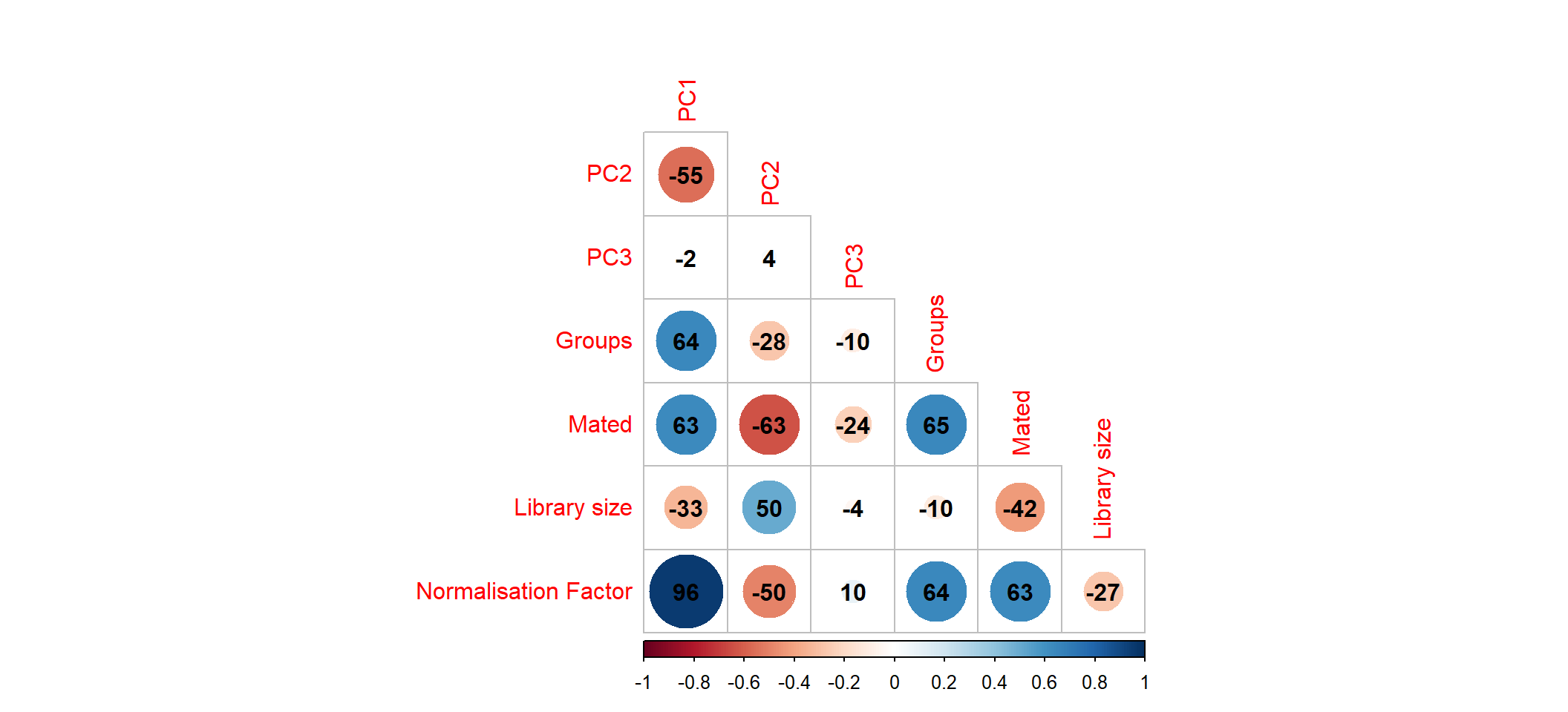
Correlation between first three principle components and measured variables
Save DGElist object
# Save DGElist object into the data/R directory
saveRDS(object = dge, file = here::here("0_data/RDS_objects/dge.rds"))
saveRDS(object = pub, file = here::here("0_data/RDS_objects/pub.rds"))

# saveRDS(object = gg_publish, file = here::here("0_data/RDS_objects/gg_publish.rds"))
sessionInfo()R version 4.2.1 (2022-06-23 ucrt)
Platform: x86_64-w64-mingw32/x64 (64-bit)
Running under: Windows 10 x64 (build 19045)
Matrix products: default
locale:
[1] LC_COLLATE=English_Australia.utf8 LC_CTYPE=English_Australia.utf8
[3] LC_MONETARY=English_Australia.utf8 LC_NUMERIC=C
[5] LC_TIME=English_Australia.utf8
attached base packages:
[1] grid stats graphics grDevices utils datasets methods
[8] base
other attached packages:
[1] Glimma_2.6.0 edgeR_3.38.4 limma_3.52.4
[4] AnnotationHub_3.4.0 BiocFileCache_2.4.0 dbplyr_2.2.1
[7] BiocGenerics_0.42.0 corrplot_0.92 cowplot_1.1.1
[10] ggrepel_0.9.1 ggbiplot_0.55 scales_1.2.1
[13] plyr_1.8.7 kableExtra_1.3.4 bookdown_0.29
[16] forcats_0.5.2 stringr_1.4.1 purrr_0.3.5
[19] tidyr_1.2.1 ggplot2_3.3.6 tidyverse_1.3.2
[22] reshape2_1.4.4 tibble_3.1.8 readr_2.1.3
[25] magrittr_2.0.3 dplyr_1.0.10
loaded via a namespace (and not attached):
[1] readxl_1.4.1 backports_1.4.1
[3] workflowr_1.7.0 systemfonts_1.0.4
[5] splines_4.2.1 BiocParallel_1.30.3
[7] GenomeInfoDb_1.32.4 digest_0.6.29
[9] htmltools_0.5.3 fansi_1.0.3
[11] memoise_2.0.1 googlesheets4_1.0.1
[13] tzdb_0.3.0 Biostrings_2.64.1
[15] annotate_1.74.0 modelr_0.1.9
[17] matrixStats_0.62.0 vroom_1.6.0
[19] svglite_2.1.0 colorspace_2.0-3
[21] blob_1.2.3 rvest_1.0.3
[23] rappdirs_0.3.3 textshaping_0.3.6
[25] haven_2.5.1 xfun_0.33
[27] crayon_1.5.2 RCurl_1.98-1.9
[29] jsonlite_1.8.2 genefilter_1.78.0
[31] survival_3.3-1 glue_1.6.2
[33] gtable_0.3.1 gargle_1.2.1
[35] zlibbioc_1.42.0 XVector_0.36.0
[37] webshot_0.5.4 DelayedArray_0.22.0
[39] DBI_1.1.3 Rcpp_1.0.9
[41] viridisLite_0.4.1 xtable_1.8-4
[43] bit_4.0.4 stats4_4.2.1
[45] htmlwidgets_1.5.4 httr_1.4.4
[47] RColorBrewer_1.1-3 ellipsis_0.3.2
[49] farver_2.1.1 pkgconfig_2.0.3
[51] XML_3.99-0.11 sass_0.4.2
[53] here_1.0.1 locfit_1.5-9.6
[55] utf8_1.2.2 labeling_0.4.2
[57] tidyselect_1.2.0 rlang_1.0.6
[59] later_1.3.0 AnnotationDbi_1.58.0
[61] munsell_0.5.0 BiocVersion_3.15.2
[63] cellranger_1.1.0 tools_4.2.1
[65] cachem_1.0.6 cli_3.4.1
[67] generics_0.1.3 RSQLite_2.2.18
[69] broom_1.0.1 evaluate_0.17
[71] fastmap_1.1.0 ragg_1.2.3
[73] yaml_2.3.5 knitr_1.40
[75] bit64_4.0.5 fs_1.5.2
[77] KEGGREST_1.36.3 whisker_0.4
[79] mime_0.12 xml2_1.3.3
[81] compiler_4.2.1 rstudioapi_0.14
[83] filelock_1.0.2 curl_4.3.3
[85] png_0.1-7 interactiveDisplayBase_1.34.0
[87] reprex_2.0.2 geneplotter_1.74.0
[89] bslib_0.4.0 stringi_1.7.8
[91] highr_0.9 lattice_0.20-45
[93] Matrix_1.5-1 vctrs_0.4.2
[95] pillar_1.8.1 lifecycle_1.0.3
[97] BiocManager_1.30.18 jquerylib_0.1.4
[99] bitops_1.0-7 httpuv_1.6.6
[101] GenomicRanges_1.48.0 R6_2.5.1
[103] promises_1.2.0.1 IRanges_2.30.1
[105] codetools_0.2-18 assertthat_0.2.1
[107] SummarizedExperiment_1.26.1 DESeq2_1.36.0
[109] rprojroot_2.0.3 withr_2.5.0
[111] S4Vectors_0.34.0 GenomeInfoDbData_1.2.8
[113] parallel_4.2.1 hms_1.1.2
[115] rmarkdown_2.17 MatrixGenerics_1.8.1
[117] googledrive_2.0.0 git2r_0.30.1
[119] Biobase_2.56.0 shiny_1.7.2
[121] lubridate_1.8.0