Orthology inference: How are genes related across Schistocerca species?
Maeva Techer
2025-06-05
Last updated: 2025-06-05
Checks: 6 1
Knit directory:
locust-comparative-genomics/
This reproducible R Markdown analysis was created with workflowr (version 1.7.1). The Checks tab describes the reproducibility checks that were applied when the results were created. The Past versions tab lists the development history.
Great! Since the R Markdown file has been committed to the Git repository, you know the exact version of the code that produced these results.
Great job! The global environment was empty. Objects defined in the global environment can affect the analysis in your R Markdown file in unknown ways. For reproduciblity it’s best to always run the code in an empty environment.
The command set.seed(20221025) was run prior to running
the code in the R Markdown file. Setting a seed ensures that any results
that rely on randomness, e.g. subsampling or permutations, are
reproducible.
Great job! Recording the operating system, R version, and package versions is critical for reproducibility.
Nice! There were no cached chunks for this analysis, so you can be confident that you successfully produced the results during this run.
Using absolute paths to the files within your workflowr project makes it difficult for you and others to run your code on a different machine. Change the absolute path(s) below to the suggested relative path(s) to make your code more reproducible.
| absolute | relative |
|---|---|
| /Users/maevatecher/Documents/GitHub/locust-comparative-genomics/data/orthofinder/Schistocerca/Results_I2/ | data/orthofinder/Schistocerca/Results_I2 |
| /Users/maevatecher/Documents/GitHub/locust-comparative-genomics/data/orthofinder/Polyneoptera/Results_I2_withDaust/ | data/orthofinder/Polyneoptera/Results_I2_withDaust |
| /Users/maevatecher/Documents/GitHub/locust-comparative-genomics/data/orthofinder/Polyneoptera/Results_I2_iqtree/ | data/orthofinder/Polyneoptera/Results_I2_iqtree |
Great! You are using Git for version control. Tracking code development and connecting the code version to the results is critical for reproducibility.
The results in this page were generated with repository version 36f043d. See the Past versions tab to see a history of the changes made to the R Markdown and HTML files.
Note that you need to be careful to ensure that all relevant files for
the analysis have been committed to Git prior to generating the results
(you can use wflow_publish or
wflow_git_commit). workflowr only checks the R Markdown
file, but you know if there are other scripts or data files that it
depends on. Below is the status of the Git repository when the results
were generated:
Ignored files:
    Ignored:    .DS_Store
    Ignored:    analysis/.DS_Store
    Ignored:    analysis/.Rhistory
    Ignored:    code/.DS_Store
    Ignored:    code/scripts/.DS_Store
    Ignored:    code/scripts/pal2nal.v14/.DS_Store
    Ignored:    data/.DS_Store
    Ignored:    data/DEG_results/.DS_Store
    Ignored:    data/DEG_results/Bulk_RNAseq/.DS_Store
    Ignored:    data/DEG_results/Bulk_RNAseq/americana/.DS_Store
    Ignored:    data/DEG_results/Bulk_RNAseq/cancellata/.DS_Store
    Ignored:    data/DEG_results/Bulk_RNAseq/cancellata/Thorax/.DS_Store
    Ignored:    data/DEG_results/Bulk_RNAseq/cubense/.DS_Store
    Ignored:    data/DEG_results/Bulk_RNAseq/davidO/.DS_Store
    Ignored:    data/DEG_results/Bulk_RNAseq/gregaria/.DS_Store
    Ignored:    data/DEG_results/Bulk_RNAseq/nitens/.DS_Store
    Ignored:    data/DEG_results/Bulk_RNAseq/piceifrons/.DS_Store
    Ignored:    data/DEG_results/RNAi/.DS_Store
    Ignored:    data/DEG_results/RNAi/All/.DS_Store
    Ignored:    data/DEG_results/RNAi/All_GFP/.DS_Store
    Ignored:    data/DEG_results/RNAi/All_control/.DS_Store
    Ignored:    data/DEG_results/RNAi/All_no_rRNA/.DS_Store
    Ignored:    data/DEG_results/RNAi/Head/.DS_Store
    Ignored:    data/DEG_results/RNAi/Head_control/.DS_Store
    Ignored:    data/DEG_results/RNAi/Head_no_rRNA/.DS_Store
    Ignored:    data/DEG_results/RNAi/Thorax/.DS_Store
    Ignored:    data/DEG_results/RNAi/Thorax_no_rRNA/.DS_Store
    Ignored:    data/DEG_results/gregaria/
    Ignored:    data/DEG_results/single_cell/.DS_Store
    Ignored:    data/WGCNA/.DS_Store
    Ignored:    data/WGCNA/input/.DS_Store
    Ignored:    data/WGCNA/input/Bulk_RNAseq/.DS_Store
    Ignored:    data/WGCNA/output/.DS_Store
    Ignored:    data/WGCNA/output/Bulk_RNAseq/.DS_Store
    Ignored:    data/behavioral_data/.DS_Store
    Ignored:    data/behavioral_data/Raw_data/.DS_Store
    Ignored:    data/list/.DS_Store
    Ignored:    data/list/Bulk_RNAseq/.DS_Store
    Ignored:    data/list/GO_Annotations/.DS_Store
    Ignored:    data/list/excluded_loci/.DS_Store
    Ignored:    data/orthofinder/.DS_Store
    Ignored:    data/orthofinder/Polyneoptera/.DS_Store
    Ignored:    data/orthofinder/Polyneoptera/Results_I2_iqtree/.DS_Store
    Ignored:    data/orthofinder/Polyneoptera/Results_I2_withDaust/.DS_Store
    Ignored:    data/orthofinder/Polyneoptera/Results_I2_withDaust/Orthogroups/.DS_Store
    Ignored:    data/orthofinder/Schistocerca/.DS_Store
    Ignored:    data/orthofinder/Schistocerca/Results_I2/.DS_Store
    Ignored:    data/orthofinder/Schistocerca/Results_I2/Orthogroups/.DS_Store
    Ignored:    data/overlap/.DS_Store
    Ignored:    data/overlap/Bulk_RNAseq/.DS_Store
    Ignored:    data/overlap/Bulk_RNAseq/cancellata/
    Ignored:    data/pathway_enrichment/.DS_Store
    Ignored:    data/pathway_enrichment/custom_sgregaria_orgdb/.DS_Store
    Ignored:    data/readcounts/.DS_Store
    Ignored:    data/readcounts/Bulk_RNAseq/.DS_Store
    Ignored:    data/readcounts/RNAi/.DS_Store

Untracked files:
    Untracked:  data/RefSeq/
Note that any generated files, e.g. HTML, png, CSS, etc., are not included in this status report because it is ok for generated content to have uncommitted changes.
These are the previous versions of the repository in which changes were
made to the R Markdown
(analysis/2_orthologs-prediction.Rmd) and HTML
(docs/2_orthologs-prediction.html) files. If you’ve
configured a remote Git repository (see ?wflow_git_remote),
click on the hyperlinks in the table below to view the files as they
were in that past version.
| File | Version | Author | Date | Message |
|---|---|---|---|---|
| Rmd | 3e696d6 | Maeva TECHER | 2025-06-05 | Adding ortho heatmap |
| html | 3e696d6 | Maeva TECHER | 2025-06-05 | Adding ortho heatmap |
| Rmd | f496e65 | Maeva TECHER | 2025-06-03 | update |
| Rmd | 4e391c3 | Maeva TECHER | 2025-05-30 | add new analysis orthology, synteny |
| html | 4e391c3 | Maeva TECHER | 2025-05-30 | add new analysis orthology, synteny |
| Rmd | cacc1db | Maeva TECHER | 2025-05-02 | updates files |
| html | cacc1db | Maeva TECHER | 2025-05-02 | updates files |
| Rmd | b982319 | Maeva TECHER | 2025-03-03 | update font |
| html | b982319 | Maeva TECHER | 2025-03-03 | update font |
| html | 34b12d4 | Maeva TECHER | 2025-02-27 | Build site. |
| Rmd | 3746422 | Maeva TECHER | 2025-02-12 | Add RNAi |
| html | 3746422 | Maeva TECHER | 2025-02-12 | Add RNAi |
| Rmd | db8b525 | Maeva TECHER | 2025-02-06 | update overlap |
| html | db8b525 | Maeva TECHER | 2025-02-06 | update overlap |
| Rmd | e55bac6 | Maeva TECHER | 2025-01-26 | Updating the github |
| html | e55bac6 | Maeva TECHER | 2025-01-26 | Updating the github |
| Rmd | faf2db3 | Maeva TECHER | 2025-01-13 | update markdown |
| html | faf2db3 | Maeva TECHER | 2025-01-13 | update markdown |
| Rmd | b80db34 | Maeva TECHER | 2025-01-13 | Adding selection analysis part |
| html | b80db34 | Maeva TECHER | 2025-01-13 | Adding selection analysis part |
| Rmd | 3fa8e62 | Maeva TECHER | 2024-11-09 | updated analysis |
| html | 3fa8e62 | Maeva TECHER | 2024-11-09 | updated analysis |
| Rmd | edb70fe | Maeva TECHER | 2024-11-08 | overlap and deg results created |
| html | edb70fe | Maeva TECHER | 2024-11-08 | overlap and deg results created |
| html | 7f1d1fe | Maeva TECHER | 2024-11-01 | Build site. |
| Rmd | f01f1cf | Maeva TECHER | 2024-11-01 | Adding new files and docs |
| html | f01f1cf | Maeva TECHER | 2024-11-01 | Adding new files and docs |
| html | ba35b82 | Maeva A. TECHER | 2024-06-20 | Build site. |
| html | c006e71 | Maeva A. TECHER | 2024-06-20 | change |
| html | 82ef59f | Maeva A. TECHER | 2024-05-16 | Build site. |
| Rmd | 151afb3 | Maeva A. TECHER | 2024-05-16 | wflow_publish("analysis/2_orthologs-prediction.Rmd") |
| html | 4dd0e26 | Maeva A. TECHER | 2024-05-15 | Build site. |
| Rmd | 38ef822 | Maeva A. TECHER | 2024-05-15 | wflow_publish("analysis/2_orthologs-prediction.Rmd") |
| html | ce82fe8 | Maeva A. TECHER | 2024-05-14 | Build site. |
| Rmd | 3ca5aee | Maeva A. TECHER | 2024-05-14 | wflow_publish("analysis/2_orthologs-prediction.Rmd") |
| html | ac06f45 | Maeva A. TECHER | 2024-05-14 | Build site. |
| Rmd | be09a11 | Maeva A. TECHER | 2024-05-14 | update markdown |
| html | be09a11 | Maeva A. TECHER | 2024-05-14 | update markdown |
| html | 0837617 | Maeva A. TECHER | 2024-01-30 | Build site. |
| html | f701a01 | Maeva A. TECHER | 2024-01-30 | reupdate |
| html | 2ca8696 | Maeva A. TECHER | 2024-01-30 | Build site. |
| html | 5c5487e | Maeva A. TECHER | 2024-01-30 | Build site. |
| html | 0135a6e | Maeva A. TECHER | 2024-01-30 | Build site. |
| Rmd | 505a8dc | Maeva A. TECHER | 2024-01-30 | wflow_publish("analysis/2_orthologs-prediction.Rmd") |
| html | 579056a | Maeva A. TECHER | 2024-01-30 | Build site. |
| Rmd | f50a3dd | Maeva A. TECHER | 2024-01-30 | wflow_publish("analysis/2_orthologs-prediction.Rmd") |
| html | f831779 | Maeva A. TECHER | 2024-01-24 | Build site. |
| html | 1b09cbe | Maeva A. TECHER | 2024-01-24 | remove |
| html | 79006db | Maeva A. TECHER | 2024-01-24 | Build site. |
| Rmd | b195f57 | Maeva A. TECHER | 2024-01-24 | refresh |
| html | b195f57 | Maeva A. TECHER | 2024-01-24 | refresh |
| html | dfc68c7 | Maeva A. TECHER | 2023-12-18 | Build site. |
| Rmd | 53877fa | Maeva A. TECHER | 2023-12-18 | add pages |
Comparative genomics and ortholog genes with OrthoFinder
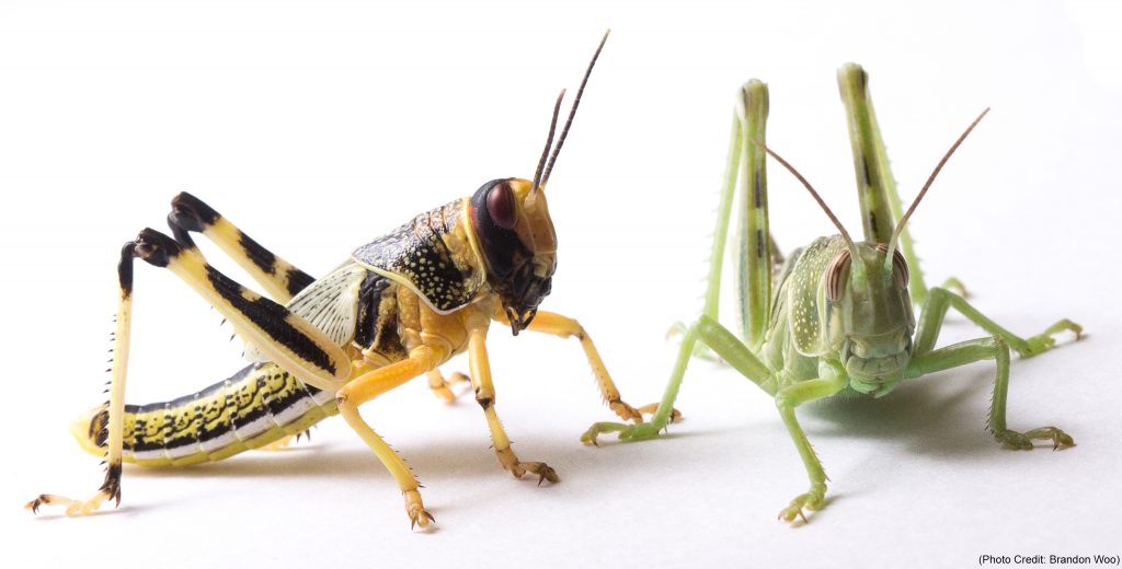
We wanted to compare the six genomes of Schistocerca to get insights on gene evolution and relationships regarding their numbers, content, function and location. In order to achieve this, we need to identify groups of orthologous genes among our species of interest, considering at least one outgroup.
Orthologs are genes from different species that originated from a single ancestral gene and evolved through speciation events. However since genes can be lost or duplicated during evolution, some genes may not have exactly one orthologue in the genome of another species. Here we will separate the 1:1 orthologs to the the concept of orthogroups. Orthogroups can contain 1:1 orthologs but also several several orthologs from different species, including paralogs and one-to-many orthologs. Paralogs are genes within the same species that have originated from a shared ancestral genes but have diverged over time following gene duplication events.
Note:We used OrthoFinder to identify the orthogroups using amino acid sequences from the longest isoform of each gene. For this part, refers to the well curated pipeline FormicidaeMolecularEvolution by Megan Barkdull (Assistant Curator of Entomology at the Natural History Museum of Los Angeles County). We describe below the modifications made and mostly copied the workflow from her Github.
1. Downloading data
We created the file “input-XXX.txt” as described to automatically download the coding sequence, protein sequence, GFF annotation data for each of our six Schistocerca species and annotated outgroups. The outgroups were choosen as close phylogenetic species with a RefSeq genome showing 1) a chromosome length, 2) associated with an annotation, 3) large size and 4) hybrid techniques used for assembly (last NCBI search: 12 May 2025).
Our target species for this study:
* The desert locust Schistocerca
gregaria
* The South American locust Schistocerca
cancellata
* The Central American locust Schistocerca
piceifrons
* The American grasshopper Schistocerca
americana
* The bird grasshopper Schistocerca
serialis cubense
* The vagrant locust Schistocerca
nitens
Our Polyneoptera outgroup species:
* The migratory locust Locusta
migratoria. Reason: Orthoptera close relative available
with chromosome length.
* The Mormon cricket Anabrus
simplex. Reason: Orthoptera close relative available
with chromosome length.
* The long cercus field cricket Gryllus
longicercus. Reason: Orthoptera close relative available
with scaffold length and a user submitted annotation.
* The two-spotted cricket Gryllus
bimaculatus. Reason: Orthoptera close relative available
with chromosome length.
* The Lord Howe Island stick insect Dryococelus
australis. Reason: Polyneoptera close relative available
with chromosome length.
* The European stick insect Bacillus
rossius redtenbacheri. Reason: Polyneoptera close
relative available with chromosome length.
* The drywood termite Cryptotermes
secundus. Reason: Eusocial insect with caste
determination phenotypic plasticity.
* The American cockroach Periplaneta
americana. Reason: Polyneoptera close relative available
with chromosome length.
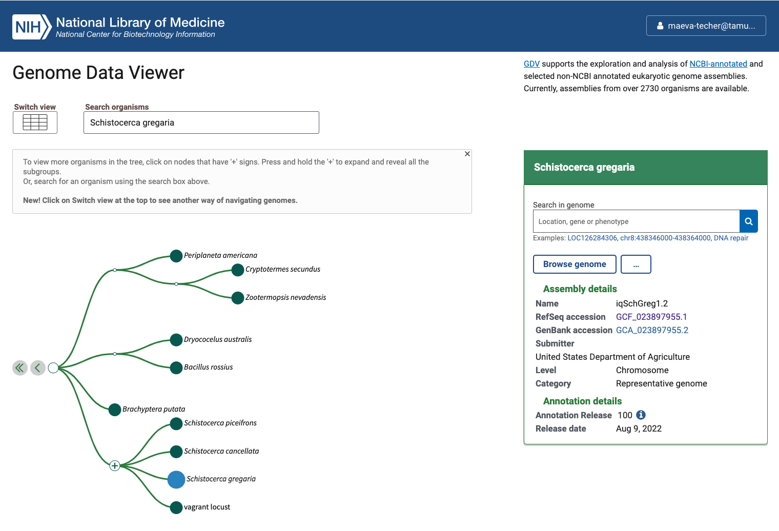
Status of Genome Data Viewer on NCBI for selecting our
outgroups
NB: During our search, we identified very valuable genomes but for which no annotation was available (e.g., CAU_Lmig_1.0 for Locusta migratoria , iqMecThal1.2 Meconema thalassinum). However upon request to NCBI team, we were informed that the Locusta genome has not been annotated because of the presence of large bacterial contamination and Meconema does not possess RNA SRAs to help with the annotation. Update Locusta migratoria The authors send us genome annotation files that they produced, but which was not working with our pipeline and seemed more limited than other genomes. Thus, Sheina Sim ran the EGAPx pipeline using a reduced SRA list that we selected across tissues and phases and using intron max size parameter of 1 million. We used the .transcripts, .proteins. and .gff files generated from this analysis.
Using the FTP NCBI link associated with each RefSeq, we created the input file.
./scripts/DataDownload ./scripts/inputurls_18polyneoptera_Nov2024.txt On the TAMU Grace cluster, when you download do not run it on a node
as it does not work. Run it from the login node or transfer the files
already preloaded. This will creates a folder ./1_RawData
with 3 files for each species.
In summary, below are the details of each RefSeq annotation that we will be using as input for OrthoFinder. It will be important to check that after steps 2-4, the number of protein coding genes OrthoFinder is similar to the initial input.
| Species | Order | Status | Genome_Size | Annotated_Genes | Protein_Coding |
|---|---|---|---|---|---|
| Schistocerca gregaria | Orthoptera | Locust | 8.7 Gb | 99467 | 19799 |
| Schistocerca cancellata | Orthoptera | Locust | 8.5 Gb | 103533 | 16907 |
| Schistocerca piceifrons | Orthoptera | Locust | 8.7 Gb | 96806 | 17490 |
| Schistocerca americana | Orthoptera | Grasshopper | 9.0 Gb | 81274 | 17662 |
| Schistocerca serialis cubense | Orthoptera | Grasshopper | 9.1 Gb | 75810 | 17237 |
| Schistocerca nitens | Orthoptera | Grasshopper | 8.8 Gb | 72560 | 17500 |
| Locusta migratoria | Orthoptera | Locust | 6.3 Gb | 0 | 0 |
| Anabrus simplex (Idaho) | Orthoptera | Outgroup | 6.4 Gb | 27091 | 14866 |
| Gryllus bimaculatus | Orthoptera | Outgroup | 1.7 Gb | 17871 | NA |
| Gryllus longicercus | Orthoptera | Outgroup | 1.9 Gb | 14831 | NA |
| Bacillus rossius redtenbacheri | Phasmatodea | Outgroup | 1.6 Gb | 19298 | 14448 |
| Dryococelus australis | Phasmatodea | Outgroup | 3.4 Gb | 33793 | NA |
| Periplaneta americana | Blattodea | Outgroup | 3.1 Gb | 28416 | 28414 |
| Cryptotermes secundus | Blattodea | Outgroup | 3.1 Gb | 27047 | NA |
2. Selecting longest isoforms
Here again, we will follow the pipeline except that to run it on Grace cluster we will make small modifications. The idea is that we will use only the single longest isoform of each gene to ease the orthology analysis. While this might not always be the principal isoform of said gene, we will apply the same bias to all genes the same way.
To run R without bothering other users, we will claim one interactive node to make sure we can proactively update the package if there are some issues:
srun --ntasks 1 --cpus-per-task 8 --mem 50G --time 05:00:00 --pty bashThen we will use any package preloaded on the cluster before needed to install our own on our user library if needed. We will need Pandoc for loading orthologr
ml GCC/13.2.0  OpenMPI/4.1.6 R_tamu/4.4.1
export R_LIBS=$SCRATCH/R_LIBS_USER/
ml Pandoc/2.13
We now simply run the script as indicated on the pipeline page:
./scripts/GeneRetrieval.R ./scripts/inputurls_13polyneoptera_May2025.txt


# the script look like this now because we added a check-step

}

library(orthologr)
library(tidyverse)
library(biomartr)
library(phylotools)
library(data.table)

# Read in the input urls file
speciesInfo <- read.table(file = args[1], sep = ",")
speciesInfo <- filter(speciesInfo, speciesInfo$V5 == "yes")
species <- speciesInfo$V4

dir.create(path = "./2_LongestIsoforms/", showWarnings = FALSE)

for (i in species) {
  print(i)
  filteredTranscriptsOutput <- paste0("./2_LongestIsoforms/", i, "_filteredTranscripts.fasta")

  if (file.exists(filteredTranscriptsOutput)) {
    message(paste("The filtered transcript file", filteredTranscriptsOutput, "already exists."))
  } else {
    proteomeFile <- paste0("./1_RawData/", i, "_proteins.faa")
    annotationFile <- paste0("./1_RawData/", i, "_GFF.gff")
    newFile <- paste0("./2_LongestIsoforms/", i, "_longestIsoforms.fasta")

    retrieve_longest_isoforms(
      proteome_file = proteomeFile,
      annotation_file = annotationFile,
      new_file = newFile,
      annotation_format = "gff"
    )

    longestIsoformsFile <- newFile
    transcriptsFile <- paste0("./1_RawData/", i, "_transcripts.fasta")

    isoforms <- phylotools::read.fasta(longestIsoformsFile)
    transcripts <- phylotools::read.fasta(transcriptsFile)

    transcripts <- separate(transcripts, col = seq.name, into = c("seq.name", "extra"), sep = " ")
    transcripts <- separate(transcripts, col = seq.name, into = c("prefix", "seq.name"), sep = "cds_")
    transcripts <- separate(transcripts, col = seq.name, into = c("seq.name", "extra"), sep = "_")
    transcripts$seq.name <- paste(transcripts$seq.name, transcripts$extra, sep = "_")

    transcripts$check <- transcripts$seq.name %in% isoforms$seq.name
    longestTranscripts <- filter(transcripts, check == TRUE)
    longestTranscripts <- select(longestTranscripts, seq.name, seq.text)

    # === NEW CHECK STEP ===
    matched_ids <- longestTranscripts$seq.name
    missing_ids <- setdiff(isoforms$seq.name, matched_ids)

    cat("✅ Matched transcripts:", length(matched_ids), "/", length(isoforms$seq.name), "\n")
    if (length(missing_ids) > 0) {
      cat("⚠️ Warning: Some isoform IDs were not matched in the transcript file.\n")
      cat("  Example missing IDs:\n")
      print(head(missing_ids, 10))
      writeLines(missing_ids, paste0("./2_LongestIsoforms/missing_cds_", i, ".txt"))
    }

    # Write output FASTA
    dat2fasta(longestTranscripts, outfile = filteredTranscriptsOutput)
  }
}
If the annotated genome is not done
by RefSeq but submitted by users:
When downloading genomes from NCBI, we found a few interesting ones that
were but annotated by users with a different format than NCBI Gnomon
pipeline. For example on the image below (when you zoom in), we can see
that the gene= field is present in RefSeq but is not in
users submitted but could be created using ID= field.
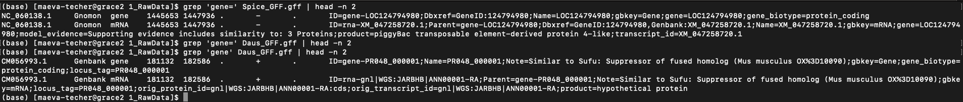
Example of difference in the presence of “gene” field between
S. piceifrons and Dryococelus australis
(3.4Gb).
To correct, I ran the following parsing code which append a new gene
column based on locus_tag:
# we need to modify the GFF, proteins and genome/transcript fasta file
sed -i 's/locus_tag=/gene=/g' {SPECIES}_GFF.gff
sed -i 's/locus_tag=/gene=/g' {SPECIES}_proteins.faa
sed -i 's/locus_tag=/gene=/g' {SPECIES}_transcripts.fasta

# then we check
grep 'gene=' {SPECIES}_GFF.gff | head -n 10
We did it for Daus_GFF.gff, Gbima_GFF.gff,
and Glong_GFF.gff. Then instead of running the
GeneRetrieval.R, we computed manually (to check if error) using the
following R script:
library(orthologr)
library(tidyverse)
library(biomartr)
library(phylotools)
library(data.table)
library(Biostrings)
library(rtracklayer)  # for importing GFF


# Define the species parameter
#species <- "Gbima" # for example
species <- "Glong"

# Define file paths based on the species parameter
proteomeFile <- paste0("./1_RawData/", species, "_proteins.faa")
annotationFile <- paste0("./1_RawData/", species, "_GFF.gff")
longestIsoformsFile <- paste0("./2_LongestIsoforms/", species, "_longestIsoforms.fasta")
transcriptsFile <- paste0("./1_RawData/", species, "_transcripts.fasta")
filteredTranscriptsOutput <- paste0("./2_LongestIsoforms/", species, "_filteredTranscripts.fasta")


# Step 1: Retrieve the longest isoforms for Glong
retrieve_longest_isoforms(
  proteome_file = proteomeFile,
  annotation_file = annotationFile,
  new_file = longestIsoformsFile,
  annotation_format = "gff"
)

# Step 2: Load longest isoforms and transcript files
isoforms <- phylotools::read.fasta(longestIsoformsFile)
isoform_ids <- isoforms$seq.name  # Get IDs of longest isoforms
isoform_ids
transcripts <- phylotools::read.fasta(transcriptsFile)
head(transcripts$seq.name)

# Step 3: Adjust headers in transcripts to match core identifiers
transcripts$seq.name <- str_extract(transcripts$seq.name, "(?<=cds_)[^ ]+")  # Extract main identifier
transcripts$seq.name <- str_extract(transcripts$seq.name, "^[^_]+")  # Keep only core ID without suffix
transcripts$seq.name

# Step 4: Filter transcripts to keep only those matching isoform IDs
filtered_transcripts <- transcripts %>%
  filter(seq.name %in% isoform_ids)

# Step 5: Report and write missing matches
matched_ids <- filtered_transcripts$seq.name
missing_ids <- setdiff(isoform_ids, matched_ids)

cat("✅ Matched transcripts:", length(matched_ids), "/", length(isoform_ids), "\n")
if (length(missing_ids) > 0) {
  cat("⚠️ Warning: Some isoform IDs were not matched in the transcript file.\n")
  cat("  Example missing IDs:\n")
  print(head(missing_ids, 10))
  writeLines(missing_ids, paste0("./2_LongestIsoforms/missing_cds_", species, ".txt"))
}

# Step 6: Write the filtered transcripts to a new FASTA file with simplified headers
phylotools::dat2fasta(filtered_transcripts, outfile = filteredTranscriptsOutput)

message("Filtered transcripts for ", species, " saved to: ", filteredTranscriptsOutput)
If the annotated genome is not done
by RefSeq but annotated by EGAPx:
I tested AGAT longest isoform and extraction of
sequences but because of different formatting, the output files were
empty. Below is the example of code I used.
#!/bin/bash

# Usage: ./agat.pipeline.sh Lmigr

set -e

SPECIES_ABBR=$1
RAW_OUT_DIR=./1_RawData
OUT_DIR=./2_LongestIsoforms

module load GCC/13.2.0 AGAT/1.4.2

echo "🔄 Working on $SPECIES_ABBR"

# Step 1: Keep only the longest isoform per gene
agat_sp_keep_longest_isoform.pl \
  -gff $RAW_OUT_DIR/${SPECIES_ABBR}_GFF.gff \
  -o $RAW_OUT_DIR/${SPECIES_ABBR}_longest_GFF.gff

# Step 2: Extract longest transcript sequences
agat_sp_extract_sequences.pl \
  --gff $RAW_OUT_DIR/${SPECIES_ABBR}_longest_GFF.gff \
  --fasta $RAW_OUT_DIR/${SPECIES_ABBR}_transcripts.fasta \
  -o $OUT_DIR/${SPECIES_ABBR}_filteredTranscripts.fasta

# Step 3: Extract longest protein sequences
agat_sp_extract_sequences.pl \
  --gff $RAW_OUT_DIR/${SPECIES_ABBR}_longest_GFF.gff \
  --fasta $RAW_OUT_DIR/${SPECIES_ABBR}_proteins.faa \
  -o $OUT_DIR/${SPECIES_ABBR}_longestIsoforms.fasta

echo "✅ $SPECIES_ABBR finished and files saved in $OUT_DIR and $RAW_OUT_DIR"
I then tailor the clean-up code for Lmigr and it worked with the following code.
cd Polyneoptera_FILA
cp Locusta_migratoria/complete.cds.fna 1_RawData/Lmigr_transcripts.fasta
cp Locusta_migratoria/complete.genomic.gff 1_RawData/Lmigr_GFF.gff
cp Locusta_migratoria/complete.proteins.faa 1_RawData/Lmigr_proteins.faa

# we need to modify the GFF, proteins and genome/transcript fasta file
# Clean GFF file: remove WGS tags and swap gene/locus_tag fields
head -n20 Lmigr_GFF.gff
sed -Ei '
  s/gnl\|WGS:[^|]+\|//g;                          # Remove gnl|WGS:ZZZZ| prefix
  s/WGS:[^:]+://g;                                # Remove WGS:ZZZZ: prefix in protein_id
  s/-R[0-9]+//g;                                  # Remove transcript isoform suffixes like -R1
  s/(^|;)locus_tag=([^;]+)/\1gene=\2/g;           # Change locus_tag= to gene=
  s/(^|;)gene=([^;]+);gene=([^;]+)/\1gene=\3/g;   # Remove duplicate gene=, keep second
' Lmigr_GFF.gff
head -n20 Lmigr_GFF.gff

# Clean protein FASTA headers (similar format to GFF)
grep ">" Lmigr_proteins.faa | head
sed -Ei '
  s/gnl\|WGS:[^|]+\|//g;
  s/WGS:[^:]+://g;
  # s/-P[0-9]+//g;
  s/-R[0-9]+//g;
  s/(^|;)locus_tag=([^;]+)/\1gene=\2/g;
  s/(^|;)gene=([^;]+);gene=([^;]+)/\1gene=\3/g;
' Lmigr_proteins.faa
grep ">" Lmigr_proteins.faa | head

# Clean and relabel transcript headers
grep ">" Lmigr_transcripts.fasta | head
sed -Ei '
  s/gnl\|WGS:[^|]+\|//g;                          # Remove gnl|WGS:ZZZZ| prefix
  s/WGS:[^:]+://g;                                # Remove WGS:ZZZZ: prefix
  # s/-P[0-9]+//g;                                # Optional: remove -P1, -P2, etc.
  s/-R[0-9]+//g;                                  # Remove -R1, -R2, etc.
  s/\[gene=([^]]+)\]/[vrac=\1]/g;                 # Temporarily rename gene= to vrac=
  s/\[locus_tag=([^]]+)\]/[gene=\1]/g;            # Change locus_tag= to gene=
  s/\[vrac=([^]]+)\]/[locus_tag=\1]/g;            # Change previous gene= to locus_tag=
' Lmigr_transcripts.fasta
grep ">" Lmigr_transcripts.fasta | head
# For the annotation GFF
sed -E 's/gnl\|WGS:ZZZZ\|//g; s/WGS:ZZZZ://g' 1_RawData/Lmigr_GFF.gff > 1_RawData/Lmigr_GFF_cleaned.gff

# For the protein FASTA
sed -E 's/^>gnl\|WGS:ZZZZ\|([^\s]+).*/>\1/' 1_RawData/Lmigr_proteins.faa > 1_RawData/Lmigr_proteins_cleaned.faa
# ============================
# Load required packages
# ============================
library(orthologr)
library(tidyverse)
library(rtracklayer)
library(Biostrings)
library(phylotools)
# ============================
# Define species and paths
# ============================
species <- "Lmigr"
proteomeFile <- paste0("./1_RawData/", species, "_proteins_cleaned.faa")
annotationFile <- paste0("./1_RawData/", species, "_GFF_cleaned.gff")
longestIsoformsFile <- paste0("./2_LongestIsoforms/", species, "_longestIsoforms.fasta")
transcriptsFile <- paste0("./1_RawData/", species, "_transcripts.fasta")
filteredTranscriptsOutput <- paste0("./2_LongestIsoforms/", species, "_filteredTranscripts.fasta")
# ============================
# Step 1: Load proteins
# ============================
proteins <- readAAStringSet(proteomeFile)
protein_ids <- names(proteins)
protein_ids_clean <- str_extract(protein_ids, "^[^ ]+")
names(proteins) <- protein_ids_clean
cat("Loaded", length(proteins), "proteins.\n")
# ============================
# Step 2: Load GFF + extract CDS info
# ============================
gff_raw <- read.delim(annotationFile, header = FALSE, sep = "\t", comment.char = "#", quote = "")
colnames(gff_raw) <- c("seqid", "source", "type", "start", "end", "score", "strand", "phase", "attributes")
cds_rows <- gff_raw[gff_raw$type == "CDS", ]
# Extract attributes
extract_attr <- function(attr, key) {
str_match(attr, paste0(key, "=([^;]+)"))[, 2]
}
cds_rows$gene <- extract_attr(cds_rows$attributes, "locus_tag")
cds_rows$protein_id <- extract_attr(cds_rows$attributes, "protein_id")
# Check ID match
gff_protein_ids <- unique(na.omit(cds_rows$protein_id))
matched <- sum(gff_protein_ids %in% protein_ids_clean)
cat("Matched:", matched, "out of", length(gff_protein_ids), "(", round(matched / length(gff_protein_ids) * 100, 2), "%)\n")
# ============================
# Step 3: Retrieve longest isoforms by CDS length
# ============================
cds_summary <- cds_rows %>%
filter(!is.na(gene) & !is.na(protein_id)) %>%
mutate(length = abs(end - start + 1)) %>%
group_by(gene, protein_id) %>%
summarise(total_length = sum(length), .groups = "drop")
longest_isoforms <- cds_summary %>%
group_by(gene) %>%
top_n(1, total_length) %>%
ungroup()
cat("Found longest isoforms for", nrow(longest_isoforms), "genes.\n")
# ============================
# Step 4: Subset and save longest isoforms
# ============================
longest_prot_ids <- longest_isoforms$protein_id
longest_prots <- proteins[names(proteins) %in% longest_prot_ids]
dir.create(dirname(longestIsoformsFile), showWarnings = FALSE)
writeXStringSet(longest_prots, filepath = longestIsoformsFile)
cat("Saved", length(longest_prots), "longest isoform protein sequences to", longestIsoformsFile, "\n")
# ============================
# Step 5: Verify transcript match
# ============================
# Load the longest isoforms FASTA to get valid IDs
longest_isoforms <- Biostrings::readAAStringSet(longestIsoformsFile)
isoform_ids <- names(longest_isoforms)
isoform_ids <- str_extract(isoform_ids, "^[^ ]+") # remove description if any
transcripts <- phylotools::read.fasta(transcriptsFile)
transcripts$protein_id <- str_extract(transcripts$seq.name, "(?<=protein_id=)[^]]+")
filtered_transcripts <- transcripts[transcripts$protein_id %in% isoform_ids, ]
# Report and write missing matches
matched_ids <- filtered_transcripts$protein_id
missing_ids <- setdiff(isoform_ids, matched_ids)
cat("✅ Matched transcripts:", length(matched_ids), "/", length(isoform_ids), "\n")
if (length(missing_ids) > 0) {
cat("⚠️ Warning: Some isoform IDs were not matched in the transcript file.\n")
cat(" Example missing IDs:\n")
print(head(missing_ids, 10))
writeLines(missing_ids, paste0("./2_LongestIsoforms/missing_cds_", species, ".txt"))
}
# Replace transcript headers with clean protein_id
filtered_transcripts$seq.name <- filtered_transcripts$protein_id
# Save filtered transcript sequences (replacing headers if needed)
filtered_transcripts_out <- filtered_transcripts[, c("seq.name", "seq.text")]
phylotools::dat2fasta(filtered_transcripts_out, outfile = filteredTranscriptsOutput)
message("Filtered transcripts for ", species, " saved to: ", filteredTranscriptsOutput)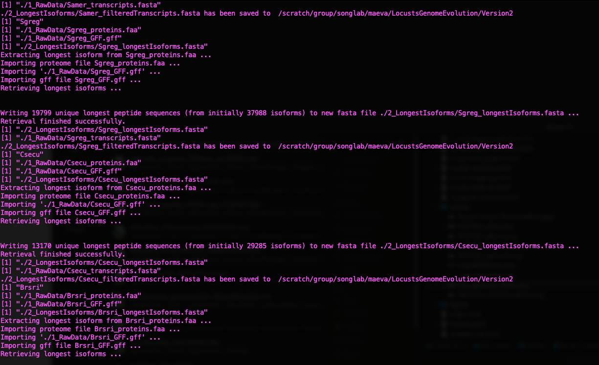
Status of Gene Retrieval script when successful
| Species | Total_Peptides | Number_Kept_Isoforms |
|---|---|---|
| Schistocerca gregaria | 37988 | 19799 |
| Schistocerca cancellata | 26362 | 16907 |
| Schistocerca piceifrons | 25717 | 17490 |
| Schistocerca americana | 26125 | 17662 |
| Schistocerca serialis cubense | 27654 | 17237 |
| Schistocerca nitens | 28445 | 17500 |
| Locusta migratoria | 33292 | 17837 |
| Anabrus simplex (Idaho) | 26037 | 14866 |
| Gryllus bimaculatus | 25032 | 17871 |
| Gryllus longicercus | 19656 | 14730 |
| Bacillus rossius redtenbacheri | 29758 | 14448 |
| Dryococelus australis | 33111 | 33111 |
| Periplaneta americana | 37240 | 16750 |
| Cryptotermes secundus | 29285 | 13170 |
3. Cleaning the raw data
For the cleaning step of the mbarkdull’s pipeline we simply followed the command line with no modifications.
./scripts/DataCleaning_modif ./scripts/inputurls_13polyneoptera_Jan2025.txt

#!/bin/bash

# Author: Maeva & ChatGPT
# Purpose: Clean headers in longestIsoforms and filteredTranscripts for all species
# Input: Files in ./2_LongestIsoforms/
# Output: Cleaned files in ./3_CleanedData/

# Create output dir if not exists
mkdir -p ./3_CleanedData

# Loop over all species files
for file in ./2_LongestIsoforms/*_filteredTranscripts.fasta; do
    # Extract species abbreviation from filename
    basename=$(basename "$file")
    species=${basename%%_filteredTranscripts.fasta}

    echo "🧬 Processing $species"

    # Define paths for both input types
    cds_in="./2_LongestIsoforms/${species}_filteredTranscripts.fasta"
    prot_in="./2_LongestIsoforms/${species}_longestIsoforms.fasta"

    # Define output names
    cds_out="./3_CleanedData/cleaned${species}_filteredTranscripts.fasta"
    prot_out="./3_CleanedData/cleaned${species}_longestIsoforms.fasta"

    # Clean headers in CDS file
    sed "s|^>|>${species}_|g" "$cds_in" |
    sed -e 's/[(|)|-]//g' > "$cds_out"

    # Clean headers in Protein file
    sed "s|^>|>${species}_|g" "$prot_in" |
    sed -e 's/[(|)|-]//g' > "$prot_out"

    # Show preview
    echo "✔ Cleaned CDS → $(head -n 1 "$cds_out")"
    echo "✔ Cleaned PROT → $(head -n 1 "$prot_out")"
    echo ""
done
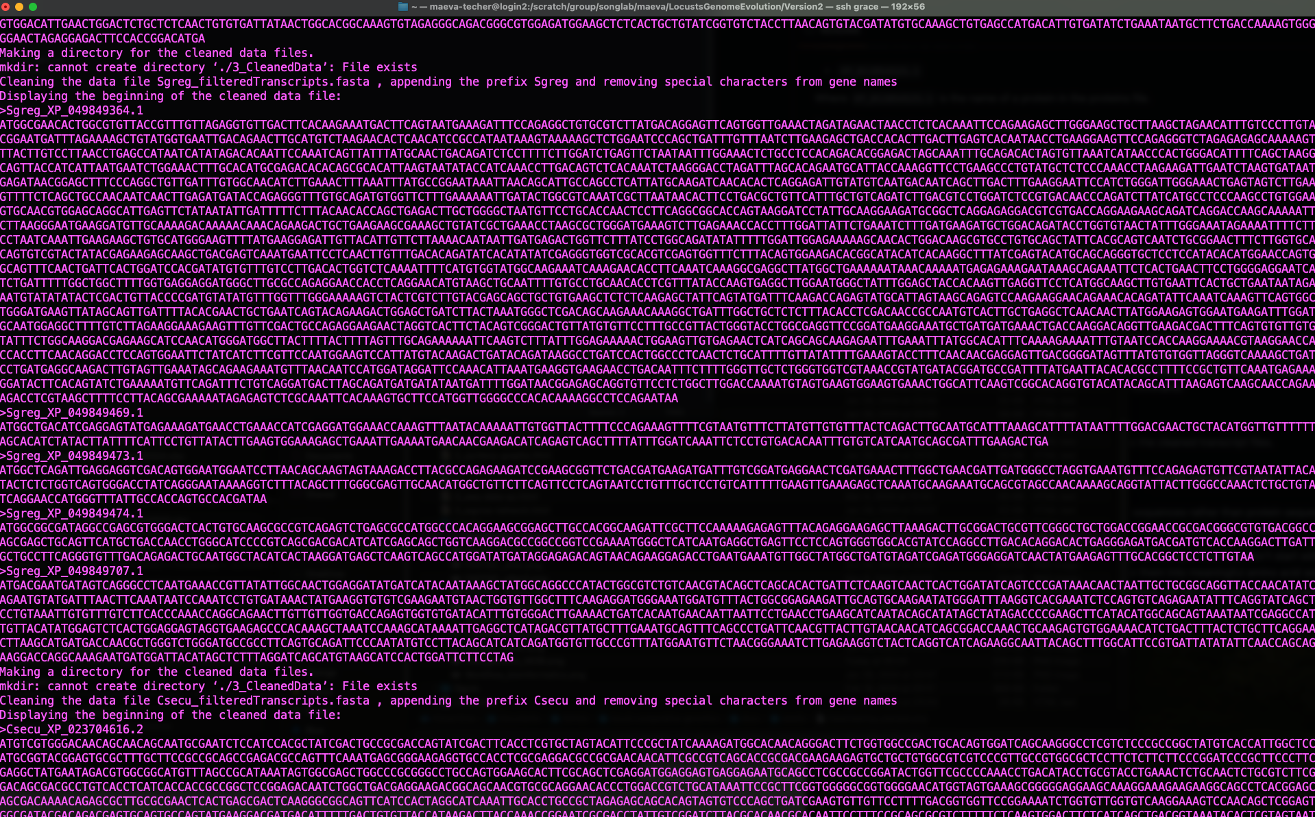
Status of Data Cleaning script when successful
4. Translating nucleotide sequences to amino acid sequences
As mentioned in the pipeline page, we will mostly need to use amino
acid sequences rather than protein and we need to translate the data we
downloaded. We can use the Python script from mbarkdull
./scripts/TranscriptFilesTranslateScript.py but here we
decided to use a conda environment after doing that
conda create -n transdecoder_env -c bioconda -c conda-forge transdecoder=5.7.1
and conda activate transdecoder_env:
#!/bin/bash

#SBATCH --job-name=Transdecoder_all_species
#SBATCH --time=04:00:00
#SBATCH --ntasks=1
#SBATCH --cpus-per-task=12
#SBATCH --mem=20G

ml Miniconda3/23.10.0-1

# Activate TransDecoder environment (via `conda run`)
export CONDA_ENV=transdecoder_env

# Prepare output folders
mkdir -p 4_1_TranslatedData/OutputFiles
mkdir -p 4_2_TransdecoderCodingSequences

# Loop over cleaned transcript files
for file in 3_CleanedData/cleaned*_filteredTranscripts.fasta; do
    base=$(basename "$file")
    abbrev=$(echo "$base" | cut -d'_' -f1 | sed 's/^cleaned//')
    rawname="${abbrev}_filteredTranscripts.fasta"

    echo "🔄 Running TransDecoder on $base..."

    # Copy to TranslatedData folder and move in
    cp "$file" "4_1_TranslatedData/$base"
    cd 4_1_TranslatedData

    # Run TransDecoder
    conda run -n $CONDA_ENV TransDecoder.LongOrfs -t "$base"
    conda run -n $CONDA_ENV TransDecoder.Predict -t "$base" --single_best_only --no_refine_starts

    pepfile="${base}.transdecoder.pep"
    cdsfile="${base}.transdecoder.cds"

    if [[ -f "$pepfile" && -f "$cdsfile" ]]; then
        echo "✅ $abbrev: TransDecoder success."

        translated_pep="translated${rawname}"
        cp "$pepfile" "OutputFiles/$translated_pep"
        sed -i 's|\.|_|g' "OutputFiles/$translated_pep"

        cp "$cdsfile" "../4_2_TransdecoderCodingSequences/cds_$rawname"
        sed -i 's|\.|_|g' "../4_2_TransdecoderCodingSequences/cds_$rawname"
    else
        echo "❌ $abbrev: TransDecoder failed. Check manually."
    fi

    cd ..
done
and then we launched the script by changing the top lines to put in sbatch:
sbatch ./scripts/DataTranslating_conda ./scripts/inputurls_13polyneoptera_Jan2025.txt Because the new names can be extra in the fasta header for
Orthofinder and later PAL2NAL we use this:
for file in *.fasta; do
    echo "Cleaning headers in $file"
    cp "$file" "${file}.original"  # Backup original
    sed -E 's/^>(\S+).*/>\1/' "$file" > tmp && mv tmp "$file"
done
This step does not seems to be really
necessary if you do not want to run HyPhy after, because Orthofinder can
immediately take the XXX_longestIsoforms.fasta files. In
that case we just run the scriptDataCleaningIsoforms_modif
on it to rename and clean it.:
5. Running Orthofinder
Now we will finally run Orthofinder to identify groups of orthologous genones in our translated amino acid sequences. We will also use MAFFT to produce multiple sequence alignment across our six species of Schistocerca and the outgroups.
Instead of using the ./scripts/DataOrthofinder from the
pipeline, we will be running our own command line here. Before doing so,
we did manually the creating of folders and moving of fasta files as
follow:
  mkdir LocustsGenomeEvolution/tmp
  mkdir -p ./5_OrthoFinder/fasta
  cp ./4_1_TranslatedData/OutputFiles/translated* ./5_OrthoFinder/fasta
#  cp ./3_CleanedData/*longestIsoforms.fasta ./5_OrthoFinder/fasta
  cd ./5_OrthoFinder/fasta
  rename translated '' translated*
  #rename _filteredTranscripts '' *_filteredTranscripts.fasta


  # We do not need to run this
  # Loop through files and rename them
for file in cleaned*_longestIsoforms.fasta; do
    # Remove "cleaned" and replace "_longestIsoforms" with "_filteredproteome"
    new_name=$(echo "$file" | sed 's/^cleaned//; s/_longestIsoforms/_filteredproteome/')
    mv "$file" "$new_name"
done
  cd ../
You can also rename them with a simple name like “S_americana.fasta”, this will help ease the visualization later on.
To run orthofinder onto our Grace cluster, we can use the following
for fasttree option but it will bug with IQ-TREE so it is
better to install with conda as recommended and the bug will be gone. I
checked the compatibility of the modules required and these are the
versions acceptable to run in
sbatchorthofinder_May2025.sh:
#!/bin/bash

##NECESSARY JOB SPECIFICATIONS
#SBATCH --job-name=orthofinder-diamond          #Set the job name to "JobExample4"
#SBATCH --time=2-00:00:00         #Set the wall clock limit to 1hr and 30min
#SBATCH --ntasks=1              #Request 1 task
#SBATCH --cpus-per-task=48       #Request 1 task
#SBATCH --mem=350G              #Request 100GB per node

#Option 1:

module purge
ml GCC/12.3.0  OpenMPI/4.1.5 OrthoFinder/2.5.5 IQ-TREE/2.3.6 FastTree/2.1.11 MAFFT/7.520-with-extensions

#or Option 2:
#conda create -n orthofinder3
#conda install bioconda::orthofinder
# make sure this install the version >3
# modify the iqtree line OrthoFinder/scripts_of/config.json
# "cmd_line": "iqtree -s INPUT -bb 1000 -pre PATH/IDENTIFIER -quiet -safe"
#check with  orthofinder -h

export CONDA_ENV=orthofinder3

proteome_dir="/scratch/group/songlab/maeva/LocustsGenomeEvolution/Polyneoptera_FINAL/5_OrthoFinder/fasta"
temporary_dir="/scratch/group/songlab/maeva/LocustsGenomeEvolution/tmp"

# Check if directories exist
if [[ ! -d $proteome_dir ]]; then
    echo "Proteome directory $proteome_dir does not exist. Exiting."
    exit 1
fi

if [[ ! -d $temporary_dir ]]; then
    echo "Temporary directory $temporary_dir does not exist. Creating it now."
    mkdir -p $temporary_dir
fi


# for conda otherwise just remove `conda run -n $CONDA_ENV `
# Run OrthoFinder
conda run -n $CONDA_ENV orthofinder -S diamond \
            -T iqtree \
            -A mafft \
            -a 12 \
            -I 1.5 \
            -t 48 \
            -M msa \
            -z \
            -f "$proteome_dir" \
            -p "$temporary_dir"
Here we use:
-S diamond DIAMOND as a sequence search program
-T iqtree IQTREE as a tree inference program
-A mafft MAFFT as the multiple sequence alignment (MSA)
program
-I 1.5 MCL inflation parameter (default from the
pipeline)
-t 32 number of threads
NOTE: The new version of OrthoFinder is doing a
light sequence trimming for alignment longer than 5000aa, so make sure
to turn off this with the -z parameter so you can conduct
HyPhy later on. Otherwise you will get a headache with PAL2NAL step!
If you expect tightly conserved orthogroups (e.g., highly conserved core genes), consider a higher inflation value (e.g., -I 2.0 or even -I 3.0). This will favor clusters with tighter connections, reducing the possibility of grouping genes that diverge functionally.
If you’re studying functionally diverse or rapidly evolving gene families (e.g., gene families with species-specific expansions), a lower inflation value (e.g., -I 1.2 to -I 1.5) may help retain related genes in the same orthogroup, even if they have evolved to some degree.
With the new version of OrthoFinder and module installation on Grace,
we now noticed that the step for tree inference stopped. Thus we need to
resuming and reroot the tree ourselves, if we received the following
error
ERROR: Species tree inference failed ERROR: An error occurred, ***please review the error messages*** they may contain useful information about the problem.
We used then the script reroot_orthofinder.sh suggested by
D. Emms using the following command:
#!/bin/bash

## SLURM job specifications
#SBATCH --job-name=manual-root-tree-orthofinder
#SBATCH --time=7-00:00:00
#SBATCH --ntasks=1
#SBATCH --cpus-per-task=4
#SBATCH --mem=30G

# Load modules
ml purge
ml GCC/12.3.0 OpenMPI/4.1.5 OrthoFinder/2.5.5 IQ-TREE/2.3.6 FastTree/2.1.11 MAFFT/7.520-with-extensions

# Check argument
if [ "$#" -ne 1 ]; then
    echo "Usage: $0 /scratch/group/songlab/maeva/LocustsGenomeEvolution/Polyneoptera_FINAL/5_OrthoFinder/fasta/Results_May20"
    exit 1
fi

# Assign input path
RESULTS_PATH=$1
ALIGN_DIR="${RESULTS_PATH}/WorkingDirectory/Alignments_ids"
ALIGN_FILE="${ALIGN_DIR}/SpeciesTreeAlignment.fa"
TREE_OUT="${ALIGN_DIR}/SpeciesTree"
TREEFILE="${TREE_OUT}.treefile"
SPECIES_ID_FILE="${RESULTS_PATH}/WorkingDirectory/SpeciesIDs.txt"
ROOTED_TREE_FILE="${RESULTS_PATH}/SpeciesTree_rooted.txt"

echo "🧬 Checking for existing IQ-TREE output..."

# Step 1: Only run IQ-TREE if output tree doesn't exist
if [ -f "$TREEFILE" ]; then
    echo "✅ IQ-TREE species tree already exists at:"
    echo "   $TREEFILE"
else
    echo "🚀 Running IQ-TREE on:"
    echo "   $ALIGN_FILE"
    iqtree2 -s "$ALIGN_FILE" \
            -bb 1000 \
            -pre "$TREE_OUT" \
            -safe -nt AUTO
fi

# Step 2: Convert Orthofinder species IDs to real names
echo "🔁 Converting Orthofinder IDs to species names..."
python convert_orthofinder_tree_ids.py "$TREEFILE" "$SPECIES_ID_FILE"
Reroot the tree manually to the correct outgroup using iTol for example and export in Newick format.
# Step 3: Replace OrthoFinder species tree with rooted version
echo "🌳 Updating OrthoFinder species tree..."
orthofinder -ft "$RESULTS_PATH" -s SpeciesTreeRooted.txt

echo "✅ All done!"
We just run the script using this:
# For example of Polyneoptera
sbatch reroot_orthofinder.sh /scratch/group/songlab/maeva/LocustsGenomeEvolution/Polyneoptera_FINAL/5_OrthoFinder/fasta/Results_May22
Now we are all done, we can explore the results and go on for the next steps.
6. Orthogroups to GeneID
At the end we obtain several folders, for which the content is extremely well explain by the software developer David Emms here.
Briefly, one of the important output in the folder
Orthogroups is the actual Orthogroups.txt
file. Although other files there are also important as we can use
Orthogroups.GeneCount.tsv for CAFE5 later on,
for example.
One of the issue with the pipeline we use is that, there will be some
suffix in front of our protein coding, so we will remove that by using
the following python code conversion_ortho.py:
ml GCCcore/12.3.0 Python/3.11.3
import re
import csv

# === Process TXT file ===
input_file_txt = 'Orthogroups.txt'
output_file_txt = 'Orthogroups_reprocessed.txt'

# Read the input file
with open(input_file_txt, 'r') as file:
    data = file.read()

# Remove all prefixes before "_XP", "_NP", and "_YP"
result = re.sub(r'\b\w+_(XP|NP|YP)', r'\1', data)

# Write the result to the output file
with open(output_file_txt, 'w') as file:
    file.write(result)

print(f"Processed data has been written to {output_file_txt}")


# === Process TSV file ===
input_file_tsv = 'Orthogroups.tsv'
output_file_tsv = 'Orthogroups_reprocessed.tsv'

# Open the input and output files
with open(input_file_tsv, 'r') as infile, open(output_file_tsv, 'w', newline='') as outfile:
    # Create CSV reader and writer for TSV
    reader = csv.reader(infile, delimiter='\t')
    writer = csv.writer(outfile, delimiter='\t')

    # Process each row
    for row in reader:
        # Modify each field in the row
        modified_row = [re.sub(r'\b\w+_(XP|NP|YP)', r'\1', field) for field in row]
        # Write the modified row to the output
        writer.writerow(modified_row)

print(f"Processed data has been written to {output_file_tsv}")
Note: Inspect the reprocessed file. I found that some protein_id have changed over time, for example some protein in nitens got an appended “_p1/7”, and some the proteins ID may have a “_1/_2” in one file and “.1/.2” in other files. Make sure to check your table after each merging.
We used the python script
python protein2geneid_generalized.py written by David to
extract the protein_id from each gene_id and make a full table with all
species. For this we need to run the script in the folder
1_RawData.
#!/usr/bin/env python3

import os
import re
import urllib.parse

# Define working and output directories
gff_directory = os.getcwd()
output_directory = os.path.join(gff_directory, "output_files")
os.makedirs(output_directory, exist_ok=True)

# List all species GFF files
species_list = [f for f in os.listdir(gff_directory) if f.endswith("_GFF.gff")]

# Define patterns to keep
keep_patterns = ["XP_", "WGS:", "gnl|", "egapx", "protein_id=", "Dbxref=NCBI_GP"]

# Loop through each species GFF file
for species_filename in species_list:
    species_name = re.sub(r"_GFF\.gff$", "", species_filename)
    input_path = os.path.join(gff_directory, species_filename)
    output_gff = os.path.join(output_directory, f"xp{species_name}.gff")
    output_tsv = os.path.join(output_directory, f"gffKey{species_name}.tsv")

    # Filter GFF lines
    with open(input_path) as fin, open(output_gff, "w") as fout:
        for line in fin:
            if any(pat in line for pat in keep_patterns):
                fout.write(line)

    print(f"Filtered lines for {species_name} → {output_gff}")

    # Parse filtered GFF into protein-to-gene map
    data = {}
    with open(output_gff) as f:
        for line in f:
            if "CDS" not in line:
                continue

            protein = (
                re.search(r"protein_id=([^;\n]+)", line) or
                re.search(r"Name=([^;\n]+)", line) or
                re.search(r"Dbxref=NCBI_GP:([^;\n]+)", line)
            )
            gene = re.search(r"gene=([^;\n]+)", line)
            product = re.search(r"product=([^;\n]+)", line)

            prot_id = protein.group(1).strip() if protein else "NA"
            gene_id = gene.group(1).strip() if gene else "NA"
            prod = urllib.parse.unquote(product.group(1).strip()) if product else "NA"

            # Fallback: use protein ID as gene ID if gene is missing
            if gene_id == "NA" and prot_id.startswith(("WGS:", "egapxtmp_")):
                gene_id = prot_id

            # Save only valid protein IDs
            if prot_id != "NA" and prot_id not in data:
                data[prot_id] = [gene_id, prod, species_name]

    # Write species-specific mapping
    with open(output_tsv, 'w') as fout:
        for prot, vals in data.items():
            fout.write(f"{prot}\t{vals[0]}\t{vals[1]}\t{vals[2]}\n")

    print(f"Saved mapping for {species_name} → {output_tsv}")

# Combine all species TSVs into one master file
final_output = os.path.join(output_directory, "allspecies_protein2geneid.tsv")
with open(final_output, "w") as fout:
    for species_filename in species_list:
        species_name = re.sub(r"_GFF\.gff$", "", species_filename)
        tsv_file = os.path.join(output_directory, f"gffKey{species_name}.tsv")
        if os.path.exists(tsv_file):
            with open(tsv_file) as fin:
                fout.write(fin.read())

print(f"✅ All species combined into {final_output}")
Launch the script as
python protein2geneid_generalized.py.
Once we have obtained both files, we can join them with R and we will have a correspondence among orthogroups_id, protein_id, gene_id, gene description and species. I had to sort the processed file by hand with excel for the first 6 Orthogroups (too long line, cutting names).
NB: I noticed there are still some small issues with the file
allspecies_protein2geneid.tsv so I fixed it by hand
afterwards. NB2: We can either filter for Schistocerca only or
we can also just run it on the Schistocerca only Orthofinder
output (difference is -I 2 vs -I 5). NB3: We need to remove this
WGS:ZZZZ: for L. migratoria
7. Orthofinder Results
Schistocerca only
library(cogeqc)
library(ggtree)
library(treeio)
library(dplyr)
library(ggplot2)
library(stringr)

# Set the base directory for your Orthofinder results
ortho_dir <- "/Users/maevatecher/Documents/GitHub/locust-comparative-genomics/data/orthofinder/Schistocerca/Results_I2/"

# Load the orthogroup file
orthogroups <- read_orthogroups(file.path(ortho_dir, "Orthogroups/Orthogroups_reprocessed.tsv"))
# Remove "_filteredTranscripts" from the Species column
orthogroups <- orthogroups %>%
  mutate(SpeciesID = str_replace(Species, "_filteredTranscripts", "")) %>%  # Clean Species name
  select(Orthogroup, SpeciesID, Gene)  # Rename and keep relevant columns

# Check the first few rows
head(orthogroups)
Orthogroup SpeciesID Gene
1 OG0000000 Samer XP_046979578.1
2 OG0000000 Samer XP_046980609.1
3 OG0000000 Samer XP_046980698.1
4 OG0000000 Samer XP_046981444.1
5 OG0000000 Samer XP_046981490.1
6 OG0000000 Samer XP_046982927.1# Load the directory with the actual stats from the Orthofinder run
ortho_stats <- read_orthofinder_stats(file.path(ortho_dir, "Comparative_Genomics_Statistics"))
ortho_stats$stats Species N_genes N_genes_in_OGs Perc_genes_in_OGs N_ssOGs
1 Samer_filteredTranscripts 17661 16918 95.8 82
2 Scanc_filteredTranscripts 16906 16008 94.7 86
3 Sgreg_filteredTranscripts 19798 18139 91.6 194
4 Snite_filteredTranscripts 16935 16215 95.7 99
5 Spice_filteredTranscripts 17489 16722 95.6 82
6 Sscub_filteredTranscripts 17236 16588 96.2 74
N_genes_in_ssOGs Perc_genes_in_ssOGs Dups
1 515 2.9 1112
2 364 2.2 966
3 721 3.6 2277
4 612 3.6 1192
5 393 2.2 1076
6 435 2.5 1008tree <- treeio::read.tree(file.path(ortho_dir, "Species_Tree/SpeciesTree_rooted_node_labels.txt"))
#tree$tip.label
#custom plot_species
plot_species_tree <- function(tree = NULL, xlim = c(0, 2), stats_list = NULL, custom_labels = NULL) {
# Basic tree plot with customized theme
p <- ggtree(tree) +
xlim(xlim) +
theme_tree() + # Use a clean theme
ggtitle("Species Tree with Duplications") + # Set a title
theme(plot.title = element_text(hjust = 0.5)) # Center the title
# Customize tip labels if provided
if (!is.null(custom_labels)) {
# Ensure length of custom_labels matches the number of tree tips
if (length(custom_labels) == length(tree$tip.label)) {
p <- p + geom_tiplab(aes(label = custom_labels), size = 4, fontface = "bold.italic", color = "darkblue")
} else {
stop("Length of custom_labels must match the number of tip labels in the tree.")
}
} else {
# Default tip labels if no custom labels are provided
p <- p + geom_tiplab(size = 4, fontface = "bold.italic", color = "darkblue")
}
if (!is.null(stats_list)) {
# Extract duplications
dups <- stats_list$duplications
dups <- dups[dups$Node %in% tree$tip.label, ] # Filter for relevant nodes
names(dups) <- c("label", "dups")
# Check for matching nodes
if (nrow(dups) > 0) {
p$data <- merge(p$data, dups, by.x = "label", by.y = "label", all.x = TRUE)
# Add duplications to the plot with larger text
p <- p +
ggtree::geom_text2(
aes(label = .data$dups),
hjust = 1.3, vjust = -0.5,
size = 5, color = "red" # Customize size and color of duplication labels
) +
labs(subtitle = "Number of Duplications per Node") # Subtitle for clarity
} else {
message("No matching nodes found for duplications.")
}
}
# Add circles around the nodes
p <- p + geom_point(size = 2, shape = 21, color = "black", fill = "black") # Circle around nodes
return(p)
}
# Plotting the tree
labels6 <- c("Schistocerca gregaria", "Schistocerca piceifrons", "Schistocerca americana", "Schistocerca serialis cubense", "Schistocerca cancellata", "Schistocerca nitens")
# Call the custom plot function with your species tree, stats, and custom labels
p<- plot_species_tree(tree, xlim = c(0, 1.5), stats_list = ortho_stats)
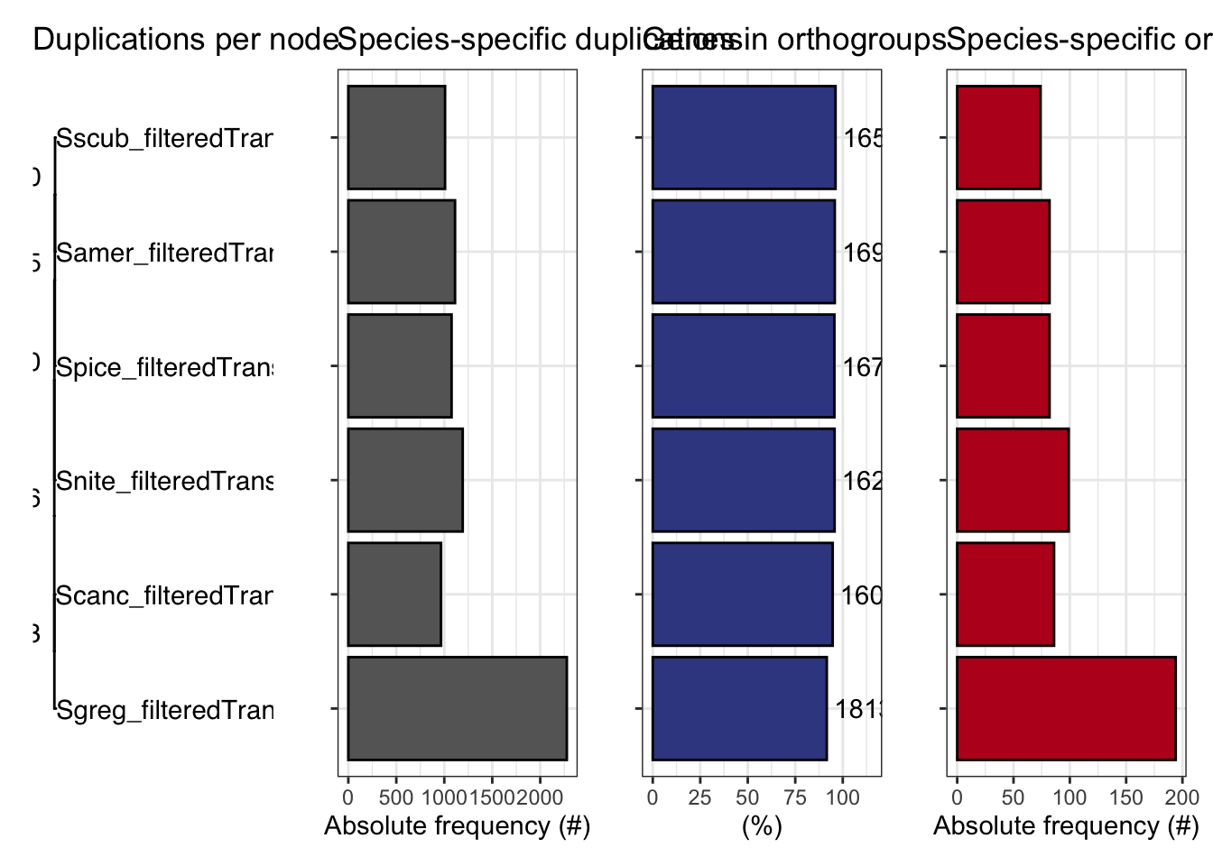
plot_duplications(ortho_stats)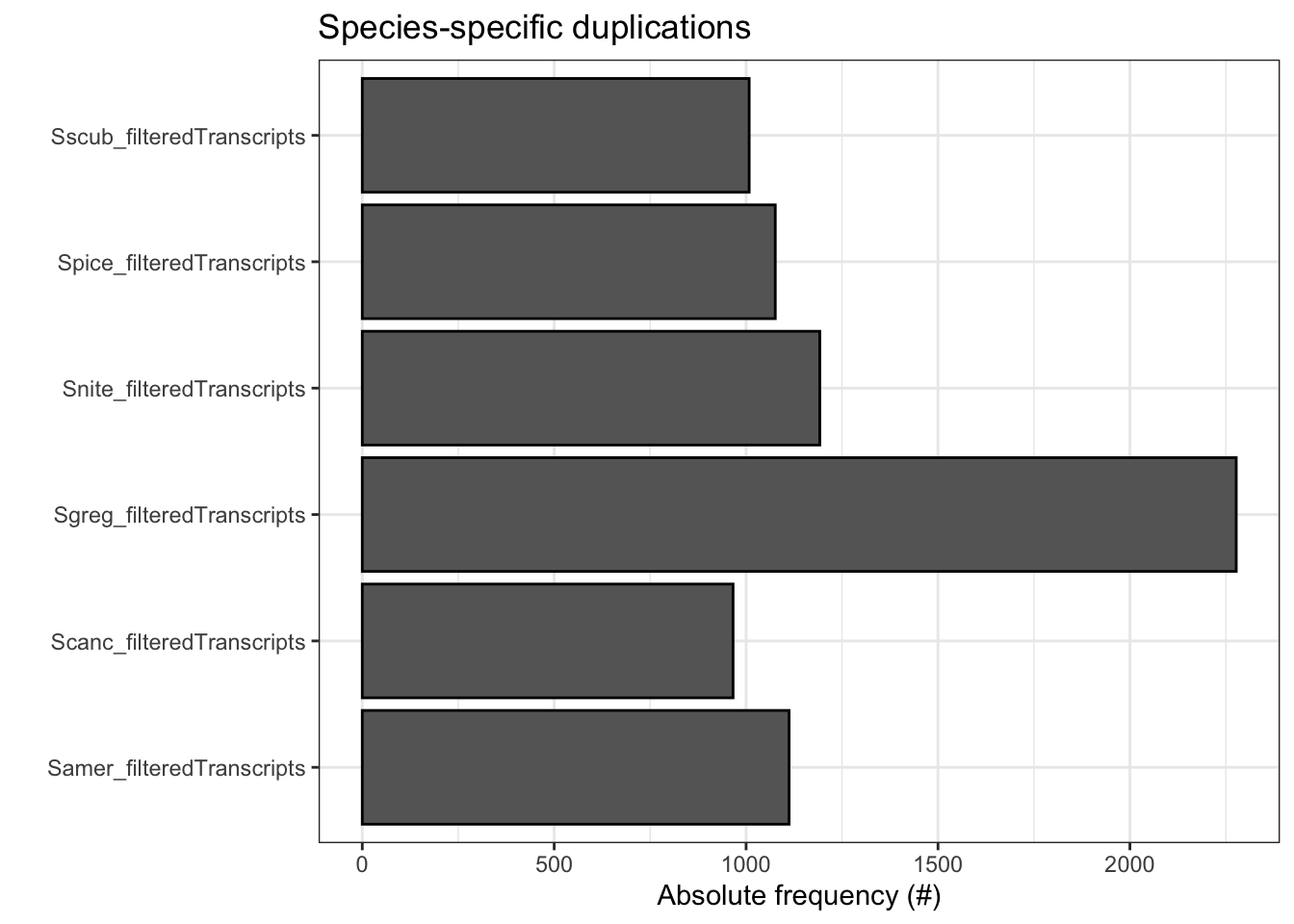
plot_genes_in_ogs(ortho_stats)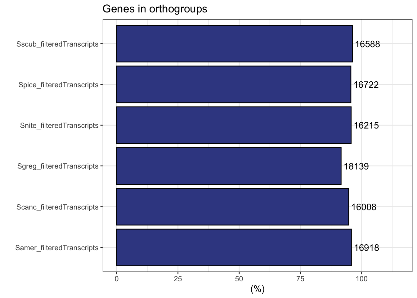
plot_species_specific_ogs(ortho_stats)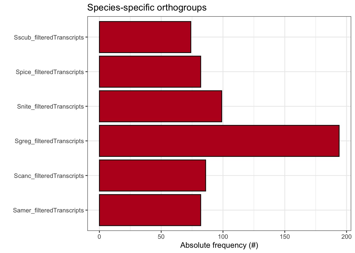
plot_orthofinder_stats(
tree = tree,
xlim = c(-0.1, 2),
stats_list = ortho_stats
)
plot_og_overlap(ortho_stats)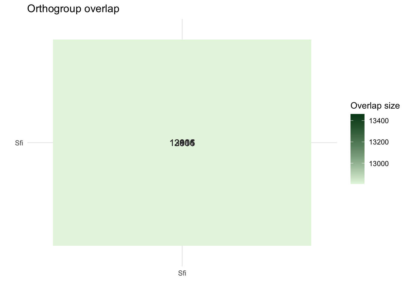
plot_og_sizes(orthogroups)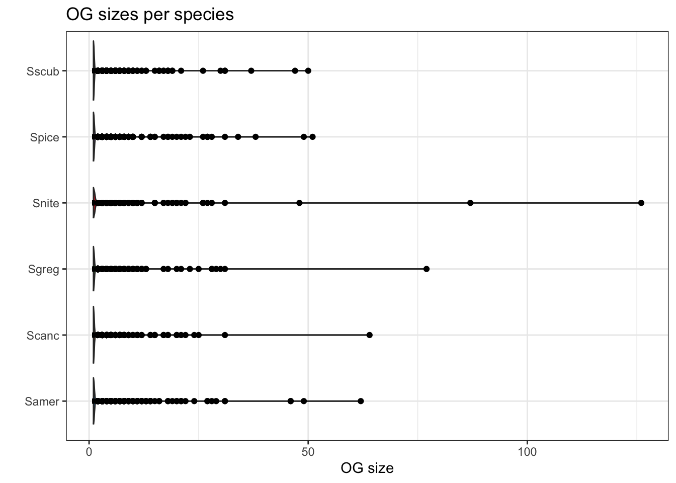
plot_og_sizes(orthogroups, log = TRUE) 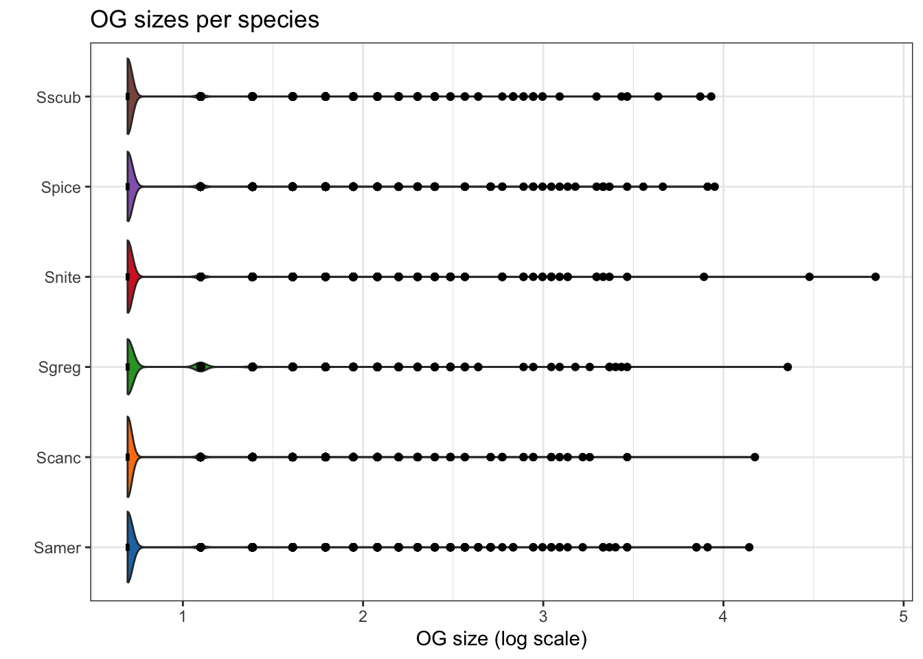
library(ggplot2)
library(dplyr)
library(tidyr)
library(stringr)
library(tibble)
# Set the base directory for your Orthofinder results
ortho_dir <- "/Users/maevatecher/Documents/GitHub/locust-comparative-genomics/data/orthofinder/Schistocerca/Results_I2/"
dResults <- paste0(ortho_dir, "Comparative_Genomics_Statistics/")
files <- c(
"OrthologuesStats_one-to-one.tsv",
"OrthologuesStats_one-to-many.tsv",
"OrthologuesStats_many-to-one.tsv",
"OrthologuesStats_many-to-many.tsv"
)
# === Function to Read and Process Data ===
read_data_matrix <- function(file_path) {
data <- read.delim(file_path, check.names = FALSE, row.names = 1)
return(as.matrix(data))
}
# === Load Data from Files ===
d11 <- read_data_matrix(paste0(dResults, files[1]))
d1m <- read_data_matrix(paste0(dResults, files[2]))
dm1 <- read_data_matrix(paste0(dResults, files[3]))
dmm <- read_data_matrix(paste0(dResults, files[4]))
# === Schistocerca Species Selection and Order ===
species <- c(
"Sscub_filteredTranscripts", # cubense
"Samer_filteredTranscripts", # americana
"Spice_filteredTranscripts", # piceifrons
"Scanc_filteredTranscripts", # cancellata
"Snite_filteredTranscripts", # nitens
"Sgreg_filteredTranscripts" # gregaria
)
# === Map Species to Readable Labels ===
species_labels <- c(
"Sscub_filteredTranscripts" = "cubense",
"Samer_filteredTranscripts" = "americana",
"Spice_filteredTranscripts" = "piceifrons",
"Scanc_filteredTranscripts" = "cancellata",
"Snite_filteredTranscripts" = "nitens",
"Sgreg_filteredTranscripts" = "gregaria"
)
# === Update Row Names ===
rownames(d11) <- species
rownames(d1m) <- species
rownames(dm1) <- species
rownames(dmm) <- species
# === Function to Prepare Data (Self-Comparison Blank) ===
combine_data <- function(d11, d1m, dm1, dmm, species, species_to_plot) {
isp <- which(species == species_to_plot)
dtot <- d11 + d1m + dm1 + dmm
data <- data.frame(
Species = species,
`1:1` = ifelse(species == species_to_plot, 0, d11[isp, ] / dtot[isp, ] * 100),
`1:many` = ifelse(species == species_to_plot, 0, d1m[isp, ] / dtot[isp, ] * 100),
`many:1` = ifelse(species == species_to_plot, 0, dm1[isp, ] / dtot[isp, ] * 100),
`many:many` = ifelse(species == species_to_plot, 0, dmm[isp, ] / dtot[isp, ] * 100)
)
return(data)
}
# === Function to Create and Save Stacked Bar Plot (Vertical) ===
create_plot <- function(data, species_to_plot, output_dir = ortho_dir) {
data_long <- data %>%
pivot_longer(
cols = -Species,
names_to = "Relationship",
values_to = "Proportion"
)
# Rename relationships to match expected levels
data_long$Relationship <- str_replace_all(data_long$Relationship, c(
"X1.1" = "1:1",
"X1.many" = "1:many",
"many.1" = "many:1",
"many.many" = "many:many"
))
# Ensure Relationship column is a factor with consistent levels
data_long$Relationship <- factor(
data_long$Relationship,
levels = c("1:1", "1:many", "many:1", "many:many")
)
# Set Custom Species Order
data_long$Species <- factor(data_long$Species, levels = species, labels = species_labels)
# Generate the Plot
plot <- ggplot(data_long, aes(x = Species, y = Proportion, fill = Relationship)) +
geom_bar(stat = "identity", position = "stack") +
scale_fill_manual(
values = c(
`1:1` = "forestgreen",
`1:many` = "orange",
`many:1` = "purple",
`many:many` = "black"
)
) +
labs(
title = paste("Orthologue multiplicty vs", species_labels[species_to_plot]),
x = "Species",
y = "Proportion (%)",
fill = "Relationship Type"
) +
theme_minimal() +
theme(
axis.text.x = element_text(angle = 45, hjust = 1),
axis.title.x = element_text(size = 12),
axis.title.y = element_text(size = 12)
)+
coord_flip()
# Save the Plot
output_file <- paste0(output_dir, "VerticalStackedBar_", species_labels[species_to_plot], ".pdf")
ggsave(output_file, plot = plot, width = 10, height = 6)
cat("Plot saved as:", output_file, "\n")
}
# === Generate Vertical Plots for Each Schistocerca Species ===
output_dir <- paste0(ortho_dir, "Plots_Schistocerca/") # Specify output directory
dir.create(output_dir, showWarnings = FALSE)
for (species_to_plot in species) {
data <- combine_data(d11, d1m, dm1, dmm, species, species_to_plot)
create_plot(data, species_to_plot, output_dir)
}Plot saved as: /Users/maevatecher/Documents/GitHub/locust-comparative-genomics/data/orthofinder/Schistocerca/Results_I2/Plots_Schistocerca/VerticalStackedBar_cubense.pdf Plot saved as: /Users/maevatecher/Documents/GitHub/locust-comparative-genomics/data/orthofinder/Schistocerca/Results_I2/Plots_Schistocerca/VerticalStackedBar_americana.pdf Plot saved as: /Users/maevatecher/Documents/GitHub/locust-comparative-genomics/data/orthofinder/Schistocerca/Results_I2/Plots_Schistocerca/VerticalStackedBar_piceifrons.pdf Plot saved as: /Users/maevatecher/Documents/GitHub/locust-comparative-genomics/data/orthofinder/Schistocerca/Results_I2/Plots_Schistocerca/VerticalStackedBar_cancellata.pdf Plot saved as: /Users/maevatecher/Documents/GitHub/locust-comparative-genomics/data/orthofinder/Schistocerca/Results_I2/Plots_Schistocerca/VerticalStackedBar_nitens.pdf Plot saved as: /Users/maevatecher/Documents/GitHub/locust-comparative-genomics/data/orthofinder/Schistocerca/Results_I2/Plots_Schistocerca/VerticalStackedBar_gregaria.pdf library(readr)
# rename for future merging
names(orthogroups)[names(orthogroups) == "Gene"] <- "protein_id"
orthogroups <- orthogroups %>%
mutate(protein_id = str_remove(protein_id, "_p[1-7]$"))
# Optional if you did not rename fasta sequence before
orthogroups$Species <- gsub("_filteredproteome", "", orthogroups$SpeciesID)
# Export the table to tab-separated text file (you can change the delimiter if needed)
output_file <- file.path(ortho_dir, "Orthogroups_Schistocerca_Jan2025.txt")
# Write the transformed data to the file
write.table(orthogroups,
file = output_file,
sep = "\t",
quote = FALSE,
row.names = FALSE)
proteingene_path <- file.path(ortho_dir, "../../../list/allspecies_protein2geneid.tsv")
proteingeneid <- read_tsv(proteingene_path, col_names = TRUE )
head(proteingeneid)# A tibble: 6 × 4
protein_id GeneID Description Species
<chr> <chr> <chr> <chr>
1 XP_047114676.1 LOC124794980 piggyBac transposable element-derived pro… Spice
2 XP_047114773.1 LOC124795035 piggyBac transposable element-derived pro… Spice
3 XP_047117829.1 LOC124798450 uncharacterized protein LOC124798450 Spice
4 XP_047118606.1 LOC124799109 RNA-binding protein 25-like Spice
5 XP_047118853.1 LOC124799306 molybdenum cofactor biosynthesis protein … Spice
6 XP_047118904.1 LOC124799809 molybdenum cofactor biosynthesis protein … Spice biotype_path <- file.path(ortho_dir, "../../../list/13polyneoptera_geneid_ncbi.csv")
biotypeid <- read_csv(biotype_path, col_names = TRUE )
head(biotypeid)# A tibble: 6 × 10
Accession Begin End Description Symbol GeneID GeneType Transcripts_accession
<chr> <dbl> <dbl> <chr> <chr> <chr> <chr> <chr>
1 NC_06468… 1 66 tRNA-Ile trnI LOC73… tRNA <NA>
2 NC_06468… 70 138 tRNA-Gln trnQ LOC73… tRNA <NA>
3 NC_06468… 138 206 tRNA-Met trnM LOC73… tRNA <NA>
4 NC_06468… 207 1227 NADH dehyd… ND2 LOC73… protein… <NA>
5 NC_06468… 1228 1295 tRNA-Trp trnW LOC73… tRNA <NA>
6 NC_06468… 1288 1350 tRNA-Cys trnC LOC73… tRNA <NA>
# ℹ 2 more variables: protein_id <chr>, Species <chr>#################
# Load Orthogroups for all genes
og_df <- read_tsv(file.path(ortho_dir, "Orthogroups/Orthogroups_reprocessed.tsv")) %>%
pivot_longer(cols = -Orthogroup, names_to = "SpeciesID", values_to = "GeneList") %>%
separate_rows(GeneList, sep = ", ") %>%
rename(GeneID = GeneList) %>%
mutate(GeneID = str_remove(GeneID, "_p[1-7]$"))
# Load list of single-copy orthogroups
single_copy_og <- read_lines(file.path(ortho_dir, "Orthogroups/Orthogroups_SingleCopyOrthologues.txt"))
og_df <- og_df %>%
mutate(
Orthogroup_Type = case_when(
Orthogroup %in% single_copy_og ~ "Single_copy",
TRUE ~ "Multi_copy"
)
)
# Load unassigned genes
unassigned_path <- file.path(ortho_dir, "Orthogroups/Orthogroups_UnassignedGenes_reprocessed.tsv")
unassigned_df <- read_tsv(unassigned_path) %>%
pivot_longer(cols = -Orthogroup, names_to = "SpeciesID", values_to = "GeneID") %>%
filter(!is.na(GeneID) & GeneID != "") %>%
mutate(Orthogroup_Type = "Unassigned")
# === Combine all three types ===
orthogroup_types_df <- bind_rows(og_df, unassigned_df) %>%
distinct(GeneID, SpeciesID, .keep_all = TRUE) %>%
rename(protein_id = GeneID) %>%
mutate(protein_id = str_remove(protein_id, "_p[1-7]$"))
# === Join with your final annotated table ===
proteinorthotable <- left_join(orthogroup_types_df, proteingeneid, by = "protein_id")
annotated_table <- left_join(proteinorthotable, biotypeid[, c("GeneID","GeneType", "Accession", "Begin", "End")], by = "GeneID")
# === Optional: keep only Schistocerca species ===
schisto_species <- c(
"Schistocerca gregaria", "Schistocerca piceifrons", "Schistocerca americana",
"Schistocerca cancellata", "Schistocerca serialis cubense", "Schistocerca nitens"
)
annotated_table <- annotated_table %>%
filter(Species %in% schisto_species)
# === Export final annotated table ===
write_csv(annotated_table, file.path(ortho_dir, "Orthogroups_genesproteinbiotype_Schistocerca_annotated_May2025.csv"))There we have it, the final table with all the corresponding IDs. This table is too big and have all species in it, so we want to reduce to only single copy orthologs and remove entries with other species than Schistocerca for now.
Polyneoptera
library(cogeqc)
library(ggtree)
library(treeio)
library(dplyr)
library(ggplot2)
library(stringr)
# Set the base directory for your Orthofinder results
#ortho_dir <- "/Users/maevatecher/Documents/GitHub/locust-comparative-genomics/data/orthofinder/Polyneoptera/Results_I2_withDaust/"
ortho_dir <- "/Users/maevatecher/Documents/GitHub/locust-comparative-genomics/data/orthofinder/Polyneoptera/Results_I2_iqtree/"
#ortho_dir <- "/Users/maevatecher/Documents/GitHub/locust-comparative-genomics/data/orthofinder/Polyneoptera/Results_I2_iqtree/"
# Load the orthogroup file
orthogroups <- read_orthogroups(file.path(ortho_dir, "Orthogroups/Orthogroups_reprocessed.tsv"))
# Remove "_filteredTranscripts" from the Species column
orthogroups <- orthogroups %>%
mutate(SpeciesID = str_replace(Species, "_filteredTranscripts", "")) %>% # Clean Species name
select(Orthogroup, SpeciesID, Gene) # Rename and keep relevant columns
# Load the directory with the actual stats from the Orthofinder run
ortho_stats <- read_orthofinder_stats(file.path(ortho_dir, "Comparative_Genomics_Statistics"))
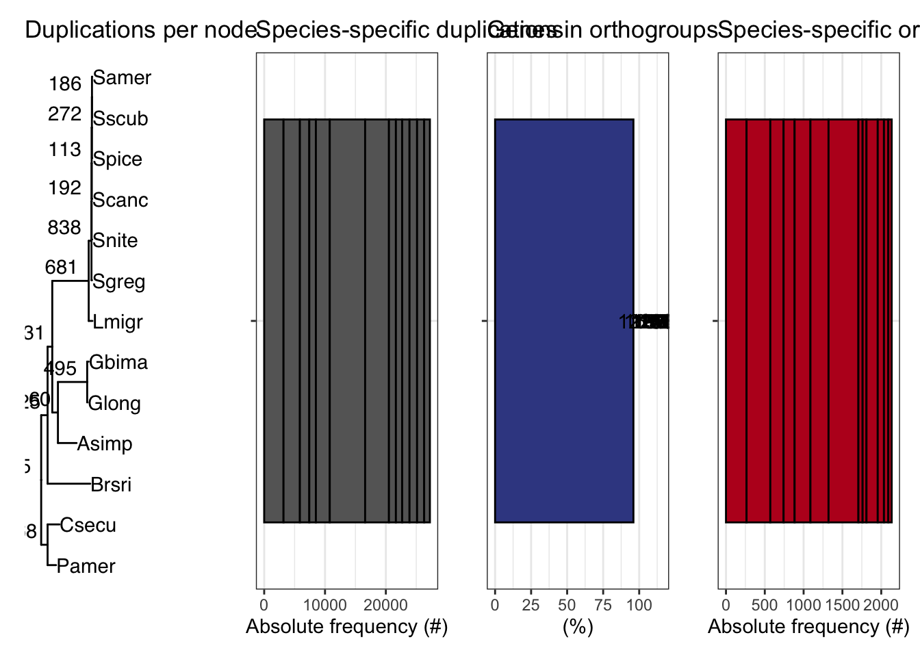
ortho_stats$stats Species N_genes N_genes_in_OGs Perc_genes_in_OGs N_ssOGs
1 Asimp_filteredTranscripts 14865 14265 96.0 265
2 Brsri_filteredTranscripts 14447 12980 89.8 306
3 Csecu_filteredTranscripts 13169 12629 95.9 171
4 Gbima_filteredTranscripts 15112 12260 81.1 142
5 Glong_filteredTranscripts 14729 13575 92.2 204
6 Lmigr_filteredTranscripts 21542 19646 91.2 233
7 Pamer_filteredTranscripts 16749 15898 94.9 385
8 Samer_filteredTranscripts 17661 17035 96.5 54
9 Scanc_filteredTranscripts 16906 16122 95.4 50
10 Sgreg_filteredTranscripts 19798 16930 85.5 145
11 Snite_filteredTranscripts 16935 16263 96.0 80
12 Spice_filteredTranscripts 17489 16783 96.0 56
13 Sscub_filteredTranscripts 17236 16656 96.6 44
N_genes_in_ssOGs Perc_genes_in_ssOGs Dups
1 1490 10.0 3178
2 1595 11.0 2689
3 800 6.1 1549
4 414 2.7 1080
5 1042 7.1 2282
6 950 4.4 5815
7 2590 15.5 3916
8 327 1.9 1142
9 172 1.0 1038
10 507 2.6 1202
11 475 2.8 1244
12 291 1.7 1165
13 240 1.4 944tree <- treeio::read.tree(file.path(ortho_dir, "Species_Tree/SpeciesTree_rooted_node_labels.txt"))
#tree$tip.label
#custom plot_species
plot_species_tree <- function(tree = NULL, xlim = c(0, 2), stats_list = NULL, custom_labels = NULL) {
# Basic tree plot with customized theme
p <- ggtree(tree) +
xlim(xlim) +
theme_tree() + # Use a clean theme
ggtitle("Species Tree with Duplications") + # Set a title
theme(plot.title = element_text(hjust = 0.5)) # Center the title
# Customize tip labels if provided
if (!is.null(custom_labels)) {
# Ensure length of custom_labels matches the number of tree tips
if (length(custom_labels) == length(tree$tip.label)) {
p <- p + geom_tiplab(aes(label = custom_labels), size = 4, fontface = "bold.italic", color = "darkblue")
} else {
stop("Length of custom_labels must match the number of tip labels in the tree.")
}
} else {
# Default tip labels if no custom labels are provided
p <- p + geom_tiplab(size = 4, fontface = "bold.italic", color = "darkblue")
}
if (!is.null(stats_list)) {
# Extract duplications
dups <- stats_list$duplications
dups <- dups[dups$Node %in% tree$tip.label, ] # Filter for relevant nodes
names(dups) <- c("label", "dups")
# Check for matching nodes
if (nrow(dups) > 0) {
p$data <- merge(p$data, dups, by.x = "label", by.y = "label", all.x = TRUE)
# Add duplications to the plot with larger text
p <- p +
ggtree::geom_text2(
aes(label = .data$dups),
hjust = 1.3, vjust = -0.5,
size = 5, color = "red" # Customize size and color of duplication labels
) +
labs(subtitle = "Number of Duplications per Node") # Subtitle for clarity
} else {
message("No matching nodes found for duplications.")
}
}
# Add circles around the nodes
p <- p + geom_point(size = 2, shape = 21, color = "black", fill = "black") # Circle around nodes
return(p)
}
# Call the custom plot function with your species tree, stats, and custom labels
p<- plot_species_tree(tree, xlim = c(0, 1.5), stats_list = ortho_stats)
plot_duplications(ortho_stats)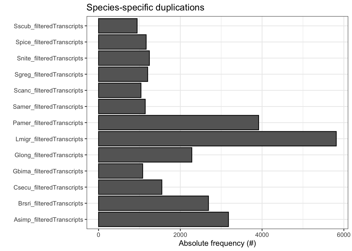
plot_genes_in_ogs(ortho_stats)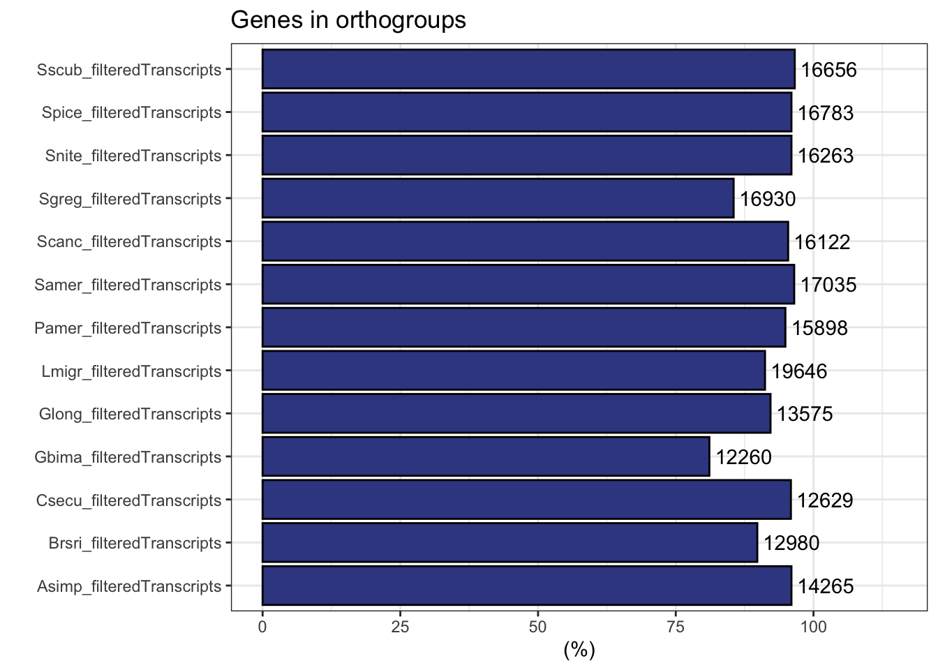
plot_species_specific_ogs(ortho_stats)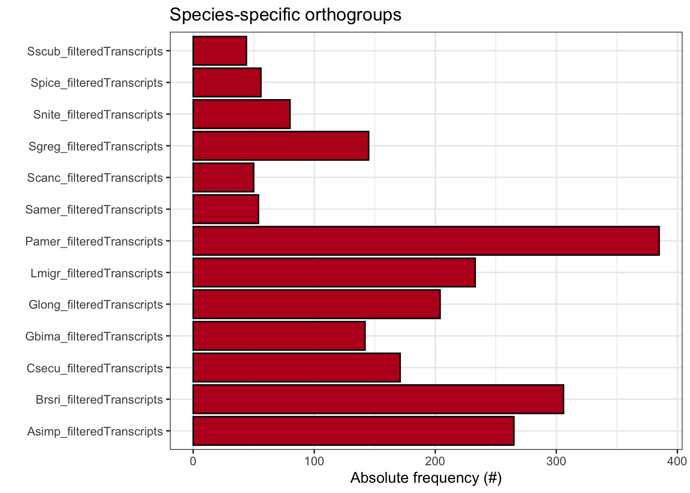
plot_orthofinder_stats(
  tree = tree,
  xlim = c(-0.1, 2),
  stats_list = ortho_stats
)
plot_og_overlap(ortho_stats)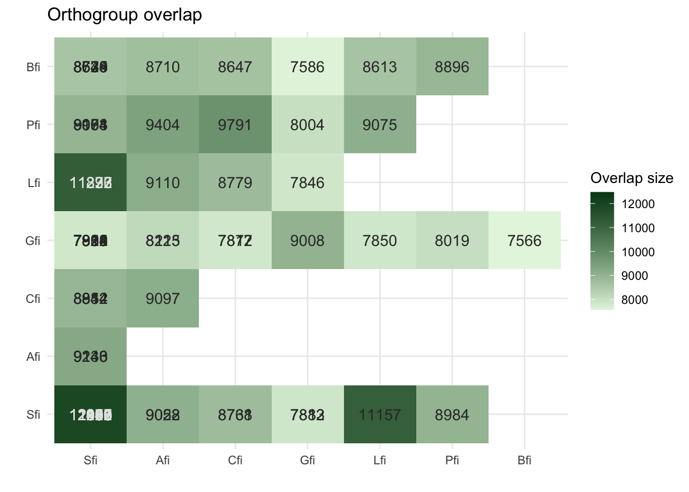
plot_og_sizes(orthogroups)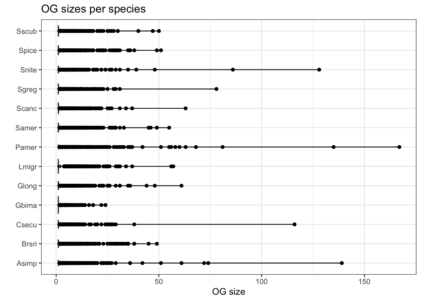
plot_og_sizes(orthogroups, log = TRUE) 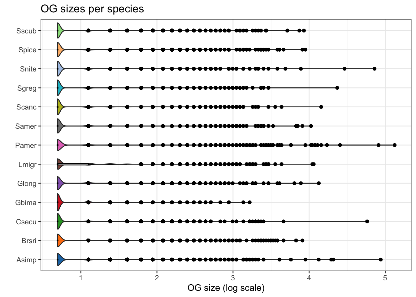
# Set the base directory for your Orthofinder results
#ortho_dir <- "/Users/maevatecher/Documents/GitHub/locust-comparative-genomics/data/orthofinder/Polyneoptera/Results_I2_withDaust/"
ortho_dir <- "/Users/maevatecher/Documents/GitHub/locust-comparative-genomics/data/orthofinder/Polyneoptera/Results_I2_iqtree/"
#ortho_dir <- "/Users/maevatecher/Documents/GitHub/locust-comparative-genomics/data/orthofinder/Polyneoptera/Results_I2_iqtree/"

dResults <- paste0(ortho_dir, "Comparative_Genomics_Statistics/")
files <- c(
  "OrthologuesStats_one-to-one.tsv",
  "OrthologuesStats_one-to-many.tsv",
  "OrthologuesStats_many-to-one.tsv",
  "OrthologuesStats_many-to-many.tsv"
)

# === Function to Read and Process Data ===
read_data_matrix <- function(file_path) {
  data <- read.delim(file_path, check.names = FALSE, row.names = 1)
  return(as.matrix(data))
}

# === Load Data from Files ===
d11 <- read_data_matrix(paste0(dResults, files[1]))
d1m <- read_data_matrix(paste0(dResults, files[2]))
dm1 <- read_data_matrix(paste0(dResults, files[3]))
dmm <- read_data_matrix(paste0(dResults, files[4]))

# === Schistocerca Species Selection and Order ===
species <- c(
  "Pamer_filteredTranscripts",
  "Csecu_filteredTranscripts",
  "Brsri_filteredTranscripts",
  "Glong_filteredTranscripts",
  "Gbima_filteredTranscripts",
  "Asimp_filteredTranscripts",
  "Sscub_filteredTranscripts",
  "Samer_filteredTranscripts",
  "Spice_filteredTranscripts",
  "Scanc_filteredTranscripts",
  "Snite_filteredTranscripts",
  "Sgreg_filteredTranscripts",
  "Lmigr_filteredTranscripts"
)

# === Map Species to Readable Labels ===
species_labels <- c(
  "Pamer_filteredTranscripts" = "P. americana",
  "Csecu_filteredTranscripts" = "C. secundus",
  "Brsri_filteredTranscripts" = "B. rossius",
  "Glong_filteredTranscripts" = "G. longicornis",
  "Gbima_filteredTranscripts" = "G. bimaculatus",
  "Asimp_filteredTranscripts" = "A. simplex",
  "Sscub_filteredTranscripts" = "cubense",
  "Samer_filteredTranscripts" = "americana",
  "Spice_filteredTranscripts" = "piceifrons",
  "Scanc_filteredTranscripts" = "cancellata",
  "Snite_filteredTranscripts" = "nitens",
  "Sgreg_filteredTranscripts" = "gregaria",
  "Lmigr_filteredTranscripts" = "L. migratoria"
)

# === Update Row Names ===
rownames(d11) <- species
rownames(d1m) <- species
rownames(dm1) <- species
rownames(dmm) <- species

# === Function to Prepare Data (Self-Comparison Blank) ===
combine_data <- function(d11, d1m, dm1, dmm, species, species_to_plot) {
  isp <- which(species == species_to_plot)
  dtot <- d11 + d1m + dm1 + dmm

  data <- data.frame(
    Species = species,
    `1:1` = ifelse(species == species_to_plot, 0, d11[isp, ] / dtot[isp, ] * 100),
    `1:many` = ifelse(species == species_to_plot, 0, d1m[isp, ] / dtot[isp, ] * 100),
    `many:1` = ifelse(species == species_to_plot, 0, dm1[isp, ] / dtot[isp, ] * 100),
    `many:many` = ifelse(species == species_to_plot, 0, dmm[isp, ] / dtot[isp, ] * 100)
  )

  return(data)
}

# === Function to Create and Save Stacked Bar Plot (Vertical) ===
create_plot <- function(data, species_to_plot, output_dir = ortho_dir) {
  data_long <- data %>%
    pivot_longer(
      cols = -Species,
      names_to = "Relationship",
      values_to = "Proportion"
    )

  # Rename relationships to match expected levels
  data_long$Relationship <- str_replace_all(data_long$Relationship, c(
    "X1.1" = "1:1",
    "X1.many" = "1:many",
    "many.1" = "many:1",
    "many.many" = "many:many"
  ))

  # Ensure Relationship column is a factor with consistent levels
  data_long$Relationship <- factor(
    data_long$Relationship,
    levels = c("1:1", "1:many", "many:1", "many:many")
  )

  # Set Custom Species Order
  data_long$Species <- factor(data_long$Species, levels = species, labels = species_labels)

  # Generate the Plot
  plot <- ggplot(data_long, aes(x = Species, y = Proportion, fill = Relationship)) +
    geom_bar(stat = "identity", position = "stack") +
    scale_fill_manual(
      values = c(
        `1:1` = "forestgreen",
        `1:many` = "orange",
        `many:1` = "purple",
        `many:many` = "black"
      )
    ) +
    labs(
      title = paste("Orthologue multiplicty vs", species_labels[species_to_plot]),
      x = "Species",
      y = "Proportion (%)",
      fill = "Relationship Type"
    ) +
    theme_minimal() +
    theme(
      axis.text.x = element_text(angle = 45, hjust = 1),
      axis.title.x = element_text(size = 12),
      axis.title.y = element_text(size = 12)
    )+
    coord_flip()

  # Save the Plot
  output_file <- paste0(output_dir, "VerticalStackedBar_", species_labels[species_to_plot], ".pdf")
  ggsave(output_file, plot = plot, width = 10, height = 6)
  cat("Plot saved as:", output_file, "\n")
}

# === Generate Vertical Plots for Each Schistocerca Species ===
output_dir <- paste0(ortho_dir, "Plots_Polyneoptera/")  # Specify output directory
dir.create(output_dir, showWarnings = FALSE)

for (species_to_plot in species) {
  data <- combine_data(d11, d1m, dm1, dmm, species, species_to_plot)
  create_plot(data, species_to_plot, output_dir)
}
Plot saved as: /Users/maevatecher/Documents/GitHub/locust-comparative-genomics/data/orthofinder/Polyneoptera/Results_I2_iqtree/Plots_Polyneoptera/VerticalStackedBar_P. americana.pdf Plot saved as: /Users/maevatecher/Documents/GitHub/locust-comparative-genomics/data/orthofinder/Polyneoptera/Results_I2_iqtree/Plots_Polyneoptera/VerticalStackedBar_C. secundus.pdf Plot saved as: /Users/maevatecher/Documents/GitHub/locust-comparative-genomics/data/orthofinder/Polyneoptera/Results_I2_iqtree/Plots_Polyneoptera/VerticalStackedBar_B. rossius.pdf Plot saved as: /Users/maevatecher/Documents/GitHub/locust-comparative-genomics/data/orthofinder/Polyneoptera/Results_I2_iqtree/Plots_Polyneoptera/VerticalStackedBar_G. longicornis.pdf Plot saved as: /Users/maevatecher/Documents/GitHub/locust-comparative-genomics/data/orthofinder/Polyneoptera/Results_I2_iqtree/Plots_Polyneoptera/VerticalStackedBar_G. bimaculatus.pdf Plot saved as: /Users/maevatecher/Documents/GitHub/locust-comparative-genomics/data/orthofinder/Polyneoptera/Results_I2_iqtree/Plots_Polyneoptera/VerticalStackedBar_A. simplex.pdf Plot saved as: /Users/maevatecher/Documents/GitHub/locust-comparative-genomics/data/orthofinder/Polyneoptera/Results_I2_iqtree/Plots_Polyneoptera/VerticalStackedBar_cubense.pdf Plot saved as: /Users/maevatecher/Documents/GitHub/locust-comparative-genomics/data/orthofinder/Polyneoptera/Results_I2_iqtree/Plots_Polyneoptera/VerticalStackedBar_americana.pdf Plot saved as: /Users/maevatecher/Documents/GitHub/locust-comparative-genomics/data/orthofinder/Polyneoptera/Results_I2_iqtree/Plots_Polyneoptera/VerticalStackedBar_piceifrons.pdf Plot saved as: /Users/maevatecher/Documents/GitHub/locust-comparative-genomics/data/orthofinder/Polyneoptera/Results_I2_iqtree/Plots_Polyneoptera/VerticalStackedBar_cancellata.pdf Plot saved as: /Users/maevatecher/Documents/GitHub/locust-comparative-genomics/data/orthofinder/Polyneoptera/Results_I2_iqtree/Plots_Polyneoptera/VerticalStackedBar_nitens.pdf Plot saved as: /Users/maevatecher/Documents/GitHub/locust-comparative-genomics/data/orthofinder/Polyneoptera/Results_I2_iqtree/Plots_Polyneoptera/VerticalStackedBar_gregaria.pdf Plot saved as: /Users/maevatecher/Documents/GitHub/locust-comparative-genomics/data/orthofinder/Polyneoptera/Results_I2_iqtree/Plots_Polyneoptera/VerticalStackedBar_L. migratoria.pdf library(readr)
# rename for future merging
names(orthogroups)[names(orthogroups) == "Gene"] <- "protein_id"
orthogroups <- orthogroups %>%
mutate(protein_id = str_remove(protein_id, "_p[1-7]$"))
# Optional if you did not rename fasta sequence before
orthogroups$Species <- gsub("_filteredproteome", "", orthogroups$Species)
# Export the table to tab-separated text file (you can change the delimiter if needed)
output_file <- file.path(ortho_dir, "Orthogroups_13species_May2025.txt")
# Write the transformed data to the file
write.table(orthogroups,
file = output_file,
sep = "\t",
quote = FALSE,
row.names = FALSE)
proteingene_path <- file.path(ortho_dir, "../../../list/allspecies_protein2geneid.tsv")
proteingeneid <- read_tsv(proteingene_path, col_names = TRUE )
head(proteingeneid)# A tibble: 6 × 4
protein_id GeneID Description Species
<chr> <chr> <chr> <chr>
1 XP_047114676.1 LOC124794980 piggyBac transposable element-derived pro… Spice
2 XP_047114773.1 LOC124795035 piggyBac transposable element-derived pro… Spice
3 XP_047117829.1 LOC124798450 uncharacterized protein LOC124798450 Spice
4 XP_047118606.1 LOC124799109 RNA-binding protein 25-like Spice
5 XP_047118853.1 LOC124799306 molybdenum cofactor biosynthesis protein … Spice
6 XP_047118904.1 LOC124799809 molybdenum cofactor biosynthesis protein … Spice biotype_path <- file.path(ortho_dir, "../../../list/13polyneoptera_geneid_ncbi.csv")
biotypeid <- read_csv(biotype_path, col_names = TRUE )
head(biotypeid)# A tibble: 6 × 10
Accession Begin End Description Symbol GeneID GeneType Transcripts_accession
<chr> <dbl> <dbl> <chr> <chr> <chr> <chr> <chr>
1 NC_06468… 1 66 tRNA-Ile trnI LOC73… tRNA <NA>
2 NC_06468… 70 138 tRNA-Gln trnQ LOC73… tRNA <NA>
3 NC_06468… 138 206 tRNA-Met trnM LOC73… tRNA <NA>
4 NC_06468… 207 1227 NADH dehyd… ND2 LOC73… protein… <NA>
5 NC_06468… 1228 1295 tRNA-Trp trnW LOC73… tRNA <NA>
6 NC_06468… 1288 1350 tRNA-Cys trnC LOC73… tRNA <NA>
# ℹ 2 more variables: protein_id <chr>, Species <chr>#################
# Load Orthogroups for all genes
og_df <- read_tsv(file.path(ortho_dir, "Orthogroups/Orthogroups_reprocessed.tsv")) %>%
pivot_longer(cols = -Orthogroup, names_to = "SpeciesID", values_to = "GeneList") %>%
separate_rows(GeneList, sep = ", ") %>%
rename(GeneID = GeneList) %>%
mutate(GeneID = str_remove(GeneID, "_p[1-7]$"))
# Load list of single-copy orthogroups
single_copy_og <- read_lines(file.path(ortho_dir, "Orthogroups/Orthogroups_SingleCopyOrthologues.txt"))
og_df <- og_df %>%
mutate(
Orthogroup_Type = case_when(
Orthogroup %in% single_copy_og ~ "Single_copy",
TRUE ~ "Multi_copy"
)
)
# Load unassigned genes
unassigned_path <- file.path(ortho_dir, "Orthogroups/Orthogroups_UnassignedGenes_reprocessed.tsv")
unassigned_df <- read_tsv(unassigned_path) %>%
pivot_longer(cols = -Orthogroup, names_to = "SpeciesID", values_to = "GeneID") %>%
filter(!is.na(GeneID) & GeneID != "") %>%
mutate(Orthogroup_Type = "Unassigned")
# === Combine all three types ===
orthogroup_types_df <- bind_rows(og_df, unassigned_df) %>%
distinct(GeneID, SpeciesID, .keep_all = TRUE) %>%
rename(protein_id = GeneID) %>%
mutate(protein_id = str_remove(protein_id, "_p[1-7]$"))
# === Join with your final annotated table ===
proteinorthotable <- left_join(orthogroup_types_df, proteingeneid, by = "protein_id")
annotated_table <- left_join(proteinorthotable, biotypeid[, c("GeneID","GeneType", "Accession", "Begin", "End")], by = "GeneID")
# === Export final annotated table ===
write_csv(annotated_table, file.path(ortho_dir, "Orthogroups_genesproteinbiotype_13species_annotated_May2025.csv"))I also create a file that is now assigning the orthogroups that originated at a clade so I can make a barplot of Schistocerca-lineage genes, Polyneoptera and so on:
library(tidyverse)

# Load and clean the GeneCounts table
gene_path <- file.path(ortho_dir, "Orthogroups/Orthogroups.GeneCount.tsv")
gene_counts <- read_tsv(gene_path) %>%
  rename_with(~ str_remove(., "_filteredTranscripts"))

# Define species per group
schistocerca <- c("Sgreg", "Snite", "Scanc", "Spice", "Sscub", "Samer")
caelifera <- c("Lmigr", schistocerca)
ensifera <- c("Asimp", "Gbima", "Glong")
outgroup <- c("Csecu", "Pamer", "Brsri")
orthoptera <- c(caelifera, ensifera)
polyneoptera <- c(orthoptera, outgroup)

# Create logical presence matrix
presence <- gene_counts %>%
  select(-Orthogroup, -Total) %>%
  mutate_all(~ . > 0)

# Count in how many species present
species_counts <- rowSums(presence)

# Count in how many species per group
in_schistocerca <- rowSums(select(presence, all_of(schistocerca))) > 0
in_caelifera <- rowSums(select(presence, all_of(caelifera))) > 0
in_ensifera <- rowSums(select(presence, all_of(ensifera))) > 0
in_outgroup <- rowSums(select(presence, all_of(outgroup))) > 0

# Count how many groups the OG spans
group_counts <- rowSums(cbind(in_schistocerca, in_caelifera & !in_schistocerca, in_ensifera, in_outgroup))

# Assign clades
gene_counts <- gene_counts %>%
  mutate(
    Species_count = species_counts,
    Assigned_Clade = case_when(
      Species_count == 1 ~ "Species_specific",
      in_schistocerca & !in_caelifera & !in_ensifera & !in_outgroup ~ "Schistocerca",
      in_caelifera & !in_ensifera & !in_outgroup ~ "Caelifera",
      in_ensifera & !in_caelifera & !in_outgroup ~ "Ensifera",
      in_caelifera & in_ensifera & !in_outgroup ~ "Orthoptera",
      in_caelifera & in_ensifera & in_outgroup ~ "Polyneoptera",
      TRUE ~ "Mixed"
    )
  )

write_tsv(gene_counts, file.path(ortho_dir, "Orthogroups/Orthogroups_CladeAssignment.tsv"))
Now we will produce a heatmap that shows the copy number variation per species using orthogroups inspired by this study on Lepidoptera gene evolution
We cleaned a bit beforehand the assignment by clade and reload the file:
library(tidyverse)
library(ComplexHeatmap)
library(circlize)
library(heatmaply)

# Schistocerca species
schisto_species <- c("Sgreg", "Snite", "Scanc", "Spice", "Samer", "Sscub")

# Load full gene counts table
gene_path <- file.path(ortho_dir, "Orthogroups/Orthogroups_CladeAssignment_cleaned.txt")
gene_counts_clade <- read_table(gene_path)

# Filter for Schistocerca and select only relevant species
df_schisto <- gene_counts_clade %>%
  filter(Assigned_Clade == "Schistocerca") %>%
  select(Orthogroup, all_of(schisto_species))

# Replace NA with 0 just in case
df_schisto[is.na(df_schisto)] <- 0

# ✅ Drop orthogroups where all values are 0
df_schisto_filtered <- df_schisto %>%
  filter(rowSums(select(., all_of(schisto_species))) > 0)

# Transpose to matrix
mat <- df_schisto_filtered %>%
  column_to_rownames("Orthogroup") %>%
  as.matrix() %>%
  t()

# Cap values at 10
mat[mat > 10] <- 10

# Sort orthogroups by total & presence
og_rank <- data.frame(
  Orthogroup = colnames(mat),
  presence = colSums(mat > 0),
  total = colSums(mat)
)

# 2. Sort: first by number of species (descending), then by total copy number (descending)
sorted_ogs <- og_rank %>%
  arrange(desc(presence), desc(total)) %>%
  pull(Orthogroup)

# 3. Reorder matrix accordingly
mat_sorted <- mat[, sorted_ogs, drop = FALSE]

# ✅ Color mapping: exact 0–10 mapping
col_fun <- structure(
  .Data = c(
    "white",       # 0
    "#CAF0F8",     # 1 - soft blue
    "#90E0EF",     # 2 - light blue
    "#00B4D8",     # 3 - turquoise
    "#0077B6",     # 4 - cyan blue
    "#03045E",     # 5 - navy
    "#7209B7",     # 6 - violet
    "#B5179E",     # 7 - magenta
    "#F72585",     # 8 - pink/red
    "#F94144",     # 9 - red
    "#D00000"      # 10 - deep red
  ),
  names = as.character(0:10)
)

# ✅ Annotation: how many species express each orthogroup
top_anno <- HeatmapAnnotation(
  Species_Present = anno_barplot(
    colSums(mat_sorted > 0),
    border = FALSE,
    gp = gpar(fill = "black"),
    height = unit(2, "cm")
  )
)

# ✅ Correct display using reordered matrix content
Heatmap(
  mat_sorted,
  name = "Copy Number",
  col = col_fun,
  cluster_rows = FALSE,
  cluster_columns = FALSE,
  top_annotation = top_anno,
  column_title = "Orthogroups (Sorted by Total Copy Number)",
  row_title = "Schistocerca Species",
  heatmap_legend_param = list(
    title = "Copy Number",
    at = 0:10,
    labels = as.character(0:10),
    color_bar = "discrete"
  )
)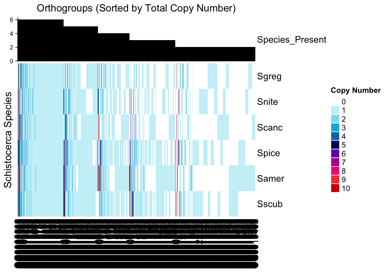
| Version | Author | Date |
|---|---|---|
| 3e696d6 | Maeva TECHER | 2025-06-05 |
# Reuse your color palette
my_colors <- c(
  "white",       # 0
  "#CAF0F8",     # 1
  "#90E0EF",     # 2
  "#00B4D8",     # 3
  "#0077B6",     # 4
  "#03045E",     # 5
  "#7209B7",     # 6
  "#B5179E",     # 7
  "#F72585",     # 8
  "#F94144",     # 9
  "#D00000"      # 10
)

# Match values 0–10 to colors
col_fun <- colorRampPalette(my_colors)(11)  # 11 breaks from 0 to 10

# Create the heatmap
heatmaply(
  mat_sorted,
  scale = "none",
  colors = col_fun,
  xlab = "Orthogroups",
  ylab = "Species",
  main = "Interactive Orthogroup Copy Number - Schistocerca",
  dendrogram = "none",
  Colv = FALSE,
  Rowv = FALSE,
  showticklabels = c(TRUE, TRUE),
  cellnote = NULL,
  hide_colorbar = FALSE,
  fontsize_row = 10,
  fontsize_col = 8
)
# Define species order
locust_species <- c("Lmigr", "Sgreg", "Snite", "Scanc", "Spice", "Samer", "Sscub")
species_order <- locust_species
# Filter orthogroups
heatmap_data <- gene_counts_clade %>%
filter(Assigned_Clade %in% c("Schistocerca", "Caelifera")) %>%
select(Orthogroup, all_of(species_order), Assigned_Clade)
# Prepare matrix
mat <- heatmap_data %>%
column_to_rownames("Orthogroup") %>%
select(-Assigned_Clade) %>%
t()
# Cap values at 10
mat[mat > 10] <- 10
# Assign clade labels
assigned_clade <- heatmap_data$Assigned_Clade
names(assigned_clade) <- heatmap_data$Orthogroup
# Separate columns by clade
schisto_cols <- names(assigned_clade[assigned_clade == "Schistocerca"])
caelifera_cols <- names(assigned_clade[assigned_clade == "Caelifera"])
# Ranking function
rank_and_sort <- function(cols) {
submat <- mat[, cols, drop = FALSE]
ranks <- data.frame(
Orthogroup = colnames(submat),
presence = colSums(submat > 0),
total = colSums(submat)
)
ordered <- ranks %>%
arrange(desc(presence), desc(total)) %>%
pull(Orthogroup)
submat[, ordered, drop = FALSE]
}
# Sort both clades
mat_schisto <- rank_and_sort(schisto_cols)
mat_caelifera <- rank_and_sort(caelifera_cols)
# Combine with Schistocerca on the right
mat_sorted <- cbind(mat_caelifera, mat_schisto)
# Annotation
annotation_col_sorted <- data.frame(
Clade = assigned_clade[colnames(mat_sorted)]
)
rownames(annotation_col_sorted) <- colnames(mat_sorted)
# Annotation colors
ann_colors <- list(
Clade = c(Schistocerca = "green", Caelifera = "skyblue2")
)
# Plot
pheatmap(
mat_sorted,
cluster_rows = FALSE,
cluster_cols = FALSE,
color = colorRampPalette(c("white", "black"))(11),
annotation_col = annotation_col_sorted,
annotation_colors = ann_colors,
fontsize_row = 10,
main = "Orthogroup Copy Number: Caelifera (left) vs Schistocerca (right)",
# cellwidth = 2, # adjust to get square cells (width)
# cellheight = 2, # adjust to get square cells (height)
gaps_row = cumsum(rep(1, length(species_order))) # creates tiny gaps between species
)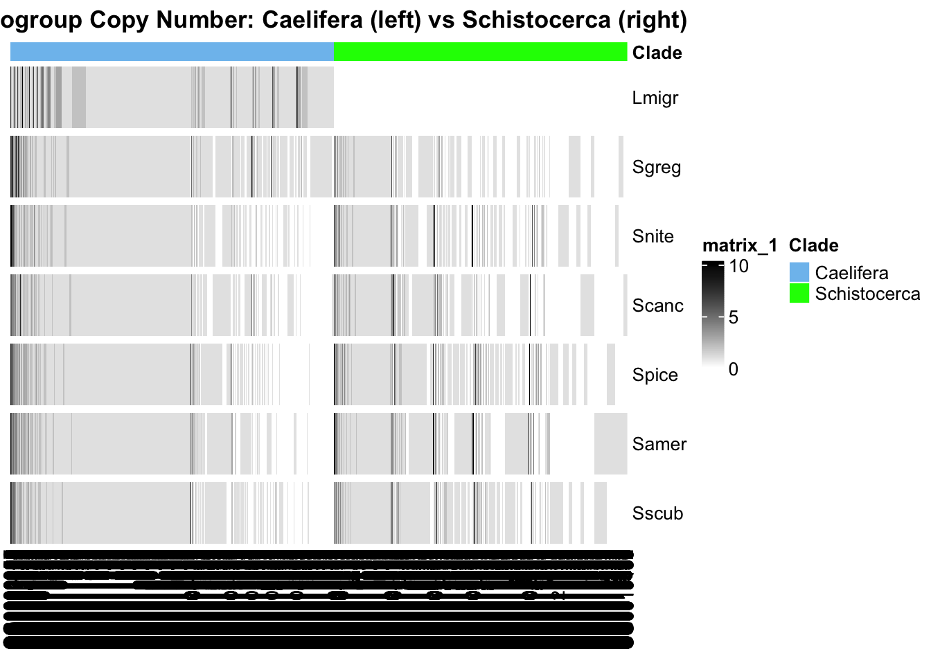
| Version | Author | Date |
|---|---|---|
| 3e696d6 | Maeva TECHER | 2025-06-05 |
References
If you use this script, and orthologr please cite:
Drost et al. 2015. Evidence for Active Maintenance of Phylotranscriptomic Hourglass Patterns in Animal and Plant Embryogenesis. Mol. Biol. Evol. 32 (5): 1221-1231. doi:10.1093/molbev/msv012
If you use Transdecoder, please cite it as:
Haas, B., and A. Papanicolaou. “TransDecoder.” (2017).
If you use Orthofinder, please cite it:
OrthoFinder’s orthogroup and ortholog inference are described here:
Emms, D.M., Kelly, S. OrthoFinder: solving fundamental biases in whole genome comparisons dramatically improves orthogroup inference accuracy. Genome Biol 16, 157 (2015).
Emms, D.M., Kelly, S. OrthoFinder: phylogenetic orthology inference for comparative genomics. Genome Biol 20, 238 (2019).
If you use the OrthoFinder species tree then also cite:
Emms D.M. & Kelly S. STRIDE: Species Tree Root Inference from Gene Duplication Events (2017), Mol Biol Evol 34(12): 3267-3278.
Emms D.M. & Kelly S. STAG: Species Tree Inference from All Genes (2018), bioRxiv https://doi.org/10.1101/267914.
Please also cite MAFFT:
K. Katoh, K. Misawa, K. Kuma, and T. Miyata. 2002. MAFFT: a novel method for rapid multiple sequence alignment based on fast Fourier transform. Nucleic Acids Res. 30(14): 3059-3066.
sessionInfo()R version 4.4.2 (2024-10-31)
Platform: aarch64-apple-darwin20
Running under: macOS Sequoia 15.5
Matrix products: default
BLAS: /Library/Frameworks/R.framework/Versions/4.4-arm64/Resources/lib/libRblas.0.dylib
LAPACK: /Library/Frameworks/R.framework/Versions/4.4-arm64/Resources/lib/libRlapack.dylib; LAPACK version 3.12.0
locale:
[1] en_US.UTF-8/en_US.UTF-8/en_US.UTF-8/C/en_US.UTF-8/en_US.UTF-8
time zone: Asia/Tokyo
tzcode source: internal
attached base packages:
[1] grid stats graphics grDevices utils datasets methods
[8] base
other attached packages:
[1] heatmaply_1.5.0 viridis_0.6.5 viridisLite_0.4.2
[4] plotly_4.10.4 circlize_0.4.16 ComplexHeatmap_2.22.0
[7] lubridate_1.9.4 forcats_1.0.0 purrr_1.0.4
[10] tidyverse_2.0.0 readr_2.1.5 tibble_3.2.1
[13] tidyr_1.3.1 stringr_1.5.1 ggplot2_3.5.2
[16] dplyr_1.1.4 treeio_1.30.0 ggtree_3.14.0
[19] cogeqc_1.10.0 kableExtra_1.4.0 knitr_1.49
[22] workflowr_1.7.1
loaded via a namespace (and not attached):
[1] RColorBrewer_1.1-3 rstudioapi_0.17.1 jsonlite_1.9.1
[4] shape_1.4.6.1 magrittr_2.0.3 magick_2.8.5
[7] ggbeeswarm_0.7.2 farver_2.1.2 rmarkdown_2.29
[10] GlobalOptions_0.1.2 fs_1.6.5 zlibbioc_1.52.0
[13] ragg_1.3.3 vctrs_0.6.5 Cairo_1.6-2
[16] webshot_0.5.5 htmltools_0.5.8.1 gridGraphics_0.5-1
[19] sass_0.4.9 bslib_0.9.0 htmlwidgets_1.6.4
[22] plyr_1.8.9 cachem_1.1.0 whisker_0.4.1
[25] igraph_2.1.4 lifecycle_1.0.4 iterators_1.0.14
[28] pkgconfig_2.0.3 R6_2.6.1 fastmap_1.2.0
[31] GenomeInfoDbData_1.2.13 clue_0.3-66 digest_0.6.37
[34] aplot_0.2.5 colorspace_2.1-1 patchwork_1.3.0
[37] S4Vectors_0.44.0 ps_1.9.0 rprojroot_2.0.4
[40] crosstalk_1.2.1 textshaping_1.0.0 seriation_1.5.7
[43] labeling_0.4.3 timechange_0.3.0 httr_1.4.7
[46] compiler_4.4.2 bit64_4.6.0-1 withr_3.0.2
[49] doParallel_1.0.17 dendextend_1.19.0 rjson_0.2.23
[52] tools_4.4.2 vipor_0.4.7 beeswarm_0.4.0
[55] ape_5.8-1 httpuv_1.6.15 glue_1.8.0
[58] callr_3.7.6 nlme_3.1-167 promises_1.3.2
[61] getPass_0.2-4 cluster_2.1.8 reshape2_1.4.4
[64] generics_0.1.3 gtable_0.3.6 tzdb_0.4.0
[67] ca_0.71.1 data.table_1.17.0 hms_1.1.3
[70] xml2_1.3.7 utf8_1.2.4 XVector_0.46.0
[73] BiocGenerics_0.52.0 foreach_1.5.2 pillar_1.10.2
[76] yulab.utils_0.2.0 vroom_1.6.5 later_1.4.1
[79] lattice_0.22-6 bit_4.5.0.1 tidyselect_1.2.1
[82] registry_0.5-1 Biostrings_2.74.1 git2r_0.35.0
[85] gridExtra_2.3 IRanges_2.40.1 svglite_2.1.3
[88] stats4_4.4.2 xfun_0.51 matrixStats_1.5.0
[91] stringi_1.8.4 UCSC.utils_1.2.0 lazyeval_0.2.2
[94] ggfun_0.1.8 yaml_2.3.10 evaluate_1.0.3
[97] codetools_0.2-20 ggplotify_0.1.2 cli_3.6.5
[100] systemfonts_1.2.1 processx_3.8.6 jquerylib_0.1.4
[103] dichromat_2.0-0.1 Rcpp_1.0.14 GenomeInfoDb_1.42.3
[106] png_0.1-8 parallel_4.4.2 assertthat_0.2.1
[109] tidytree_0.4.6 scales_1.4.0 crayon_1.5.3
[112] GetoptLong_1.0.5 rlang_1.1.6 TSP_1.2-5