Cortisol Concentration Values, Test4
Paloma Contreras
2025-04-24
Last updated: 2025-04-24
Checks: 6 1
Knit directory:
HairCort-Evaluation-Nist2020/
This reproducible R Markdown analysis was created with workflowr (version 1.7.1). The Checks tab describes the reproducibility checks that were applied when the results were created. The Past versions tab lists the development history.
The R Markdown file has unstaged changes. To know which version of
the R Markdown file created these results, you’ll want to first commit
it to the Git repo. If you’re still working on the analysis, you can
ignore this warning. When you’re finished, you can run
wflow_publish to commit the R Markdown file and build the
HTML.
Great job! The global environment was empty. Objects defined in the global environment can affect the analysis in your R Markdown file in unknown ways. For reproduciblity it’s best to always run the code in an empty environment.
The command set.seed(20241016) was run prior to running
the code in the R Markdown file. Setting a seed ensures that any results
that rely on randomness, e.g. subsampling or permutations, are
reproducible.
Great job! Recording the operating system, R version, and package versions is critical for reproducibility.
Nice! There were no cached chunks for this analysis, so you can be confident that you successfully produced the results during this run.
Great job! Using relative paths to the files within your workflowr project makes it easier to run your code on other machines.
Great! You are using Git for version control. Tracking code development and connecting the code version to the results is critical for reproducibility.
The results in this page were generated with repository version dd200fc. See the Past versions tab to see a history of the changes made to the R Markdown and HTML files.
Note that you need to be careful to ensure that all relevant files for
the analysis have been committed to Git prior to generating the results
(you can use wflow_publish or
wflow_git_commit). workflowr only checks the R Markdown
file, but you know if there are other scripts or data files that it
depends on. Below is the status of the Git repository when the results
were generated:
Ignored files:
    Ignored:    .DS_Store
    Ignored:    .RData
    Ignored:    .Rhistory
    Ignored:    analysis/.DS_Store
    Ignored:    analysis/.Rhistory
    Ignored:    data/.DS_Store
    Ignored:    data/Test3/.DS_Store
    Ignored:    data/Test4/.DS_Store

Unstaged changes:
    Modified:   analysis/ELISA_Analysis_FinalVals_test4.Rmd
    Modified:   analysis/ELISA_Calc_FinalVals_test4.Rmd
    Modified:   data/Test4/Data_Cortisol_Processed.csv
    Modified:   data/Test4/Data_QC_flagged.csv
    Modified:   data/Test4/Data_cort_values_methodB.csv
    Modified:   data/Test4/Data_cort_values_methodC.csv
    Modified:   data/Test4/Data_cort_values_method_ALL.csv
Note that any generated files, e.g. HTML, png, CSS, etc., are not included in this status report because it is ok for generated content to have uncommitted changes.
These are the previous versions of the repository in which changes were
made to the R Markdown
(analysis/ELISA_Calc_FinalVals_test4.Rmd) and HTML
(docs/ELISA_Calc_FinalVals_test4.html) files. If you’ve
configured a remote Git repository (see ?wflow_git_remote),
click on the hyperlinks in the table below to view the files as they
were in that past version.
| File | Version | Author | Date | Message |
|---|---|---|---|---|
| Rmd | dd200fc | Paloma | 2025-04-23 | corrected figures |
| html | dd200fc | Paloma | 2025-04-23 | corrected figures |
| Rmd | 7240d2e | Paloma | 2025-04-22 | organized files |
| html | 7240d2e | Paloma | 2025-04-22 | organized files |
| Rmd | 82ad928 | Paloma | 2025-04-17 | upd |
| html | 82ad928 | Paloma | 2025-04-17 | upd |
| Rmd | 16ce91c | Paloma | 2025-04-10 | recalc_evaluations |
| html | 16ce91c | Paloma | 2025-04-10 | recalc_evaluations |
| html | bbb70a9 | Paloma | 2025-04-09 | comparing methods |
| Rmd | ccad031 | Paloma | 2025-04-09 | new_calc |
| html | ccad031 | Paloma | 2025-04-09 | new_calc |
| html | 77c2ab5 | Paloma | 2025-04-08 | cleaning test3 |
| Rmd | ced6eed | Paloma | 2025-04-03 | upd |
| html | ced6eed | Paloma | 2025-04-03 | upd |
| Rmd | ca6c804 | Paloma | 2025-04-03 | new calc final vals |
| html | ca6c804 | Paloma | 2025-04-03 | new calc final vals |
| Rmd | 528855b | Paloma | 2025-04-03 | new_calc |
| html | 528855b | Paloma | 2025-04-03 | new_calc |
Summary
Cortisol value calculations (includes bad quality samples, n = 41)
| Min. | 1st Qu. | Median | Mean | 3rd Qu. | Max. | NA’s | |
|---|---|---|---|---|---|---|---|
| A) Standard Method (mult. by sample dilution) | 17.13 | 29.01 | 32.27 | 35.28 | 39.47 | 82.94 | 4 |
| B) Spike-Corrected Method (Nist 2020) | -45.870 | -35.833 | -5.960 | -3.488 | 23.109 | 50.963 | 4 |
| C) Spike-Corrected (Sam’s Method) | 7.472 | 18.533 | 24.559 | 27.009 | 31.196 | 80.804 | 4 |
Cortisol value calculations (removed bad quality samples)
| Min. | 1st Qu. | Median | Mean | 3rd Qu. | Max. | |
|---|---|---|---|---|---|---|
| A) Standard Method (mult. by sample dilution) | 18.27 | 29.27 | 31.54 | 34.13 | 37.73 | 69.17 |
| B) Spike-Corrected Method (Nist 2020) | -39.371 | -34.855 | -20.577 | -14.325 | -6.825 | 40.400 |
| C) Spike-Corrected (Sam’s Method) | ** 11.80** | 18.45 | 24.09 | 24.05 | 30.32 | 40.40 |
Results:
Intra-assay CV: 14.5%
Intra-assay CV after removing low quality samples: 10%
Inter-assay CV: 21% (Bindings for 20mg sample diluted in 250 uL, no spike: 64.8% and 48% in test3 and test4, respectively)
Conclusions:
Concerns: Overall quality of the plate is not great, but serial dilusions show clear parallelism and standards have values within the expected
Explanation of each variable used in calculations
Ave_Conc_pg/ml: average ELISA reading per sample in pg/mL
Weight_mg: hair weight in mg
Buffer_nl: assay buffer volume in nL → we convert to mL
Spike: binary indicator (1 = spiked sample)
SpikeVol_uL: volume of spike added in µL
Dilution: dilution factor (already present)
Vol_in_well.tube_uL: total volume in well/tube in µL (for spike correction)
std: standard reading value
extraction: methanol volume ratio = vol added / vol recovered (e.g. 1/0.75 ml)
Cortisol concentration calculations
#practice
Ave_Conc_pg.ml <- 4617
Spike_contribution <- 0
Weight_mg <- 50
Extraction_ratio <- 1.3/1
Buffer_ml <- 0.25

((Ave_Conc_pg.ml - Spike_contribution) /  # (A - spike)
       Weight_mg) *                                    # / B *
     Extraction_ratio *                               # C / D *
      Buffer_ml
[1] 30.0105# 31.19476
Ave_Conc_pg.ml / Weight_mg * Extraction_ratio * Buffer_ml [1] 30.0105# 31.19476((A/B) * (C/D) * E * 10,000 * SLd) = F
Parameters and unit transformations:
# Volume of methanol used for cortisol extraction varies, so it is included in file
# as Extraction_ratio (vol added / vol recovered) in mL

# Reading of spike standard and conversion to ug/dl
std <- (3191 + 3228) / 2 # test 4 backfit
std.r <- std / 10000 # std in ul/dl

# Creating variables in indicated units
df$Buffer_ml <- c(df$Buffer_nl/1000) # dilution (buffer)
df$Ave_Conc_ug.dl <- c(df$Ave_Conc_pg.ml/10000) # Transform to μg/dl from assay output
Identify and flag bad quality samples
        ABOVE 80% binding                   HIGH CV HIGH CV;ABOVE 80% binding
                        4                         2                         7
HIGH CV;UNDER 20% binding                        OK         UNDER 20% binding
                        1                        60                         8
(A) Standard Calculation
Formula:
((A/B) * (C/D) * E * 10,000) = F
- A = μg/dl from assay output;
- B = weight (in mg) of hair subjected to extraction;
- C = vol. (in ml) of methanol added to the powdered hair;
- D = vol. (in ml) of methanol recovered from the extract and subsequently dried down;
- E = vol. (in ml) of assay buffer used to reconstitute the dried extract;
- F = final value of hair CORT Concentration in pg/mg
##################################
##### Calculate final values #####
##################################

data$Final_pg.mg_A <- c(
    ((data$Ave_Conc_ug.dl) / data$Weight_mg) *             # A/B *
      data$Extraction_ratio *                              # C/D  *
      data$Buffer_ml * 10000)       # E * 10000
Summary of all samples (n = 37 ): Min. 1st Qu. Median Mean 3rd Qu. Max.
0.4198 1.9653 7.6554 16.0868 30.5653 69.1712 Summary for good quality samples only (n = 18 ): Min. 1st Qu. Median Mean 3rd Qu. Max.
2.077 4.696 7.861 16.287 17.877 69.171 (B) Accounting for Spike
We followed the procedure described in Nist et al. 2020:
“Thus, after pipetting 25μL of standards and samples into the appropriate wells of the 96-well assay plate, we added 25μL of the 0.333ug/dL standard to all samples, resulting in a 1:2 dilution of samples. The remainder of the manufacturer’s protocol was unchanged. We analyzed the assay plate in a Powerwave plate reader (BioTek, Winooski, VT) at 450nm and subtracted background values from all assay wells. In the calculations, we subtracted the 0.333ug/dL standard reading from the sample readings. Samples that resulted in a negative number were considered nondetectable. We converted cortisol levels from ug/dL, as measured by the assay, to pg/mg—based on the mass of hair collected and analyzed using the following formula:
A/B * C/D * E * 10,000 * 2 = F
where
- A = μg/dl from assay output;
- B = weight (in mg) of collected hair;
- C = vol. (in ml) of methanol added to the powdered hair;
- D = vol. (in ml) of methanol recovered from the extract and subsequently dried down;
- E = vol. (in ml) of assay buffer used to reconstitute the dried extract; 10,000 accounts for changes in metrics; 2 accounts for the dilution factor after addition of the spike; and
- F = final value of hair cortisol concentration in pg/mg”
- SPd = sample dilution factor (if serially diluted)
##################################
##### Calculate final values #####
##################################

# spike is already divided by 10000 (unit is ug/dL)
data$Final_pg.mg_B <-
  ifelse(
    data$Spike == 1,                                         ## Only spiked samples
      ((data$Ave_Conc_ug.dl - (std.r)) /                     # (A-spike)
        data$Weight_mg)                                      # / B
        * data$Extraction_ratio *                            # C / D
        data$Buffer_ml * 10000 * 2,   # E * 10000 * 2
        data$Final_pg.mg_A
    )
Summary all samples: Min. 1st Qu. Median Mean 3rd Qu. Max.
-45.870 -35.833 -5.960 -10.952 7.547 31.196 Summary good quality samples only: Min. 1st Qu. Median Mean 3rd Qu. Max.
-39.371 -34.855 -20.577 -19.549 -6.825 7.655 (C) Sam’s calculation
Simplifies unnecessary unit transformations and accounts for spike considering dilution of both sample and the spike
- Step 1: Calculate contribution of the spike
- Step 2: Substract spike from plate reading values and calculate final values accounting for dilution of the sample, weight, and reconstitution
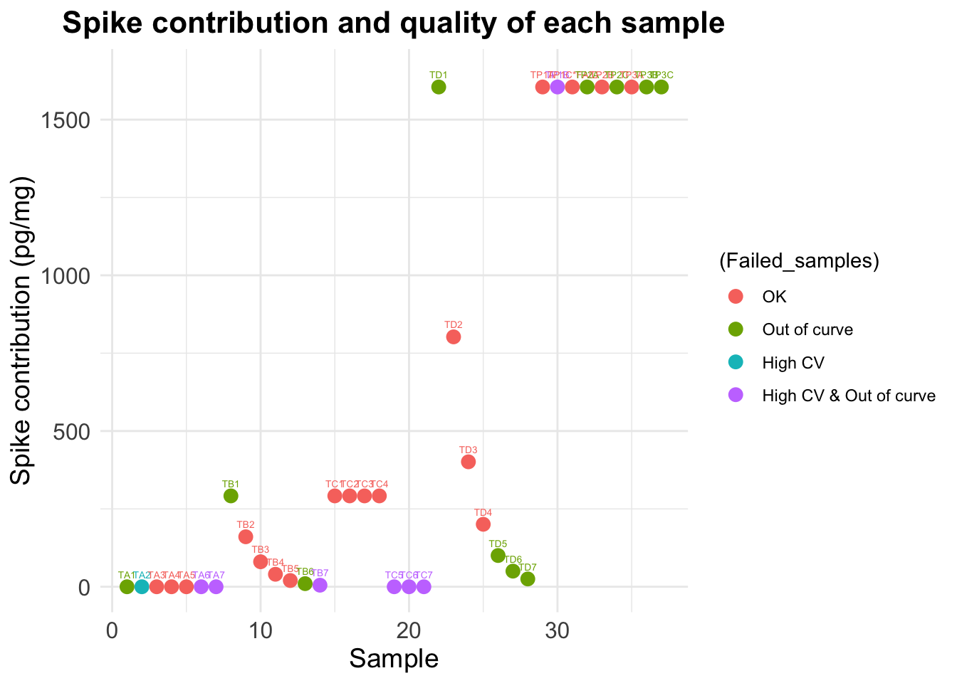
Step 1: Calculate contribution of spike
X * Y / Z / SPd = SP
- SP = final value of spike contribution in pg/mL
- X = volume of spike added (mL)
- Y = concentration of the spike added (pg/mL)
- SPd = if serially diluted, dilution factor for the spike (i.e: 1, 2, 4, 8, etc.)
- Z = total volume (mL) in the well or tube, if spike is added before loading the plate (sample + spike)
# Transforming units
data$SpikeVol_ml <- data$SpikeVol_ul/1000                 # X to mL
data$Vol_in_well.tube_ml <- data$Vol_in_well.tube_ul/1000 # Z to mL

# Calculate spike contribution to each sample
      ##  ( Spike vol. x Spike Conc.)
      ##   ------------------------  / dilution = Spike contribution
      ##        Total vol.

# Calculate cort contribution of spike to each sample
data$Spike_contribution <- ((data$SpikeVol_ml * std  /     # X * Y
                            data$Vol_in_well.tube_ml) /  # Z /
                              data$Dilution_spike)       # SP
The reading for standard 1 in this plate is 3209.5The total contribution of the Spike to each sample is can be any of the following numbers (in pg/ml) [1] 0.000000 291.772727 160.475000 80.237500 40.118750 20.059375
[7] 10.029688 5.014844 1604.750000 802.375000 401.187500 200.593750
[13] 100.296875 50.148438 25.074219 1604.750000Step 2 : Substract spike and calculate final values
((A - SP)/B) * (C/D) * E * SLd = F
- A = pg/ml from assay output;
- SP = spike contribution (in pg/ml)
- B = weight (in mg) of hair subjected to extraction;
- C = vol. (in ml) of methanol added to the powdered hair;
- D = vol. (in ml) of methanol recovered from the extract and subsequently dried down;
- E = vol. (in ml) of assay buffer used to reconstitute the dried extract;
- F = final value of hair CORT Concentration in pg/mg.
##################################
##### Calculate final values #####
##################################

data$Final_pg.mg_C <-
     (((data$Ave_Conc_pg.ml - data$Spike_contribution)) /  # (A - spike)
      data$Weight_mg) *                                    # / B *
     data$Extraction_ratio *                               # C / D *
      data$Buffer_ml                                       # E
head(data)
Wells Sample Category Binding.Perc Ave_Conc_ug.dl Ave_Conc_pg.ml Weight_mg
1 C3 TA1 A 14.0 0.46170 4617.0 50
2 E3 TA2 A 22.4 0.29210 2921.0 50
3 G3 TA3 A 44.3 0.11330 1133.0 50
4 A4 TA4 A 55.2 0.07474 747.4 50
5 C4 TA5 A 74.1 0.03524 352.4 50
6 E4 TA6 A 84.2 0.02260 226.0 50
Buffer_ml Spike SpikeVol_ul Dilution_sample Dilution_spike Extraction_ratio
1 0.25 0 0 1 1 1.351351
2 0.25 0 0 2 1 1.351351
3 0.25 0 0 4 1 1.351351
4 0.25 0 0 8 1 1.351351
5 0.25 0 0 16 1 1.351351
6 0.25 0 0 32 1 1.351351
Vol_in_well.tube_ul Failed_samples Final_pg.mg_A Final_pg.mg_B
1 50 Out of curve 31.195946 31.195946
2 50 High CV 19.736486 19.736486
3 50 OK 7.655405 7.655405
4 50 OK 5.050000 5.050000
5 50 OK 2.381081 2.381081
6 50 High CV & Out of curve 1.527027 1.527027
SpikeVol_ml Vol_in_well.tube_ml Spike_contribution Final_pg.mg_C
1 0 0.05 0 31.195946
2 0 0.05 0 19.736486
3 0 0.05 0 7.655405
4 0 0.05 0 5.050000
5 0 0.05 0 2.381081
6 0 0.05 0 1.527027Summary for all samples: Min. 1st Qu. Median Mean 3rd Qu. Max.
0.2335 1.5270 6.7184 10.3434 18.0378 32.2815 Summary for good quality samples only: Min. 1st Qu. Median Mean 3rd Qu. Max.
1.943 3.461 7.069 9.283 13.188 29.414 | Sample | Final_pg.mg_A | Final_pg.mg_B | Final_pg.mg_C | Spike_contribution | Binding.Perc | SpikeVol_ul | Dilution_sample | Dilution_spike | Extraction_ratio | |
|---|---|---|---|---|---|---|---|---|---|---|
| 32 | TP2A | 33.71556 | 10.373333 | 19.45111 | 1604.75 | 17.3 | 25 | 1 | 1 | 1.333333 |
| 33 | TP2B | 27.56444 | -1.928889 | 13.30000 | 1604.75 | 21.1 | 25 | 1 | 1 | 1.333333 |
| 34 | TP2C | 32.30222 | 7.546667 | 18.03778 | 1604.75 | 18.1 | 25 | 1 | 1 | 1.333333 |
| 35 | TP3A | 69.17117 | -20.686937 | 29.41385 | 1604.75 | 23.2 | 25 | 1 | 1 | 1.351351 |
| 36 | TP3B | 28.06667 | 13.340000 | 17.36833 | 1604.75 | 15.5 | 25 | 1 | 1 | 1.333333 |
| 37 | TP3C | 31.07333 | 19.353333 | 20.37500 | 1604.75 | 13.9 | 25 | 1 | 1 | 1.333333 |
Plots
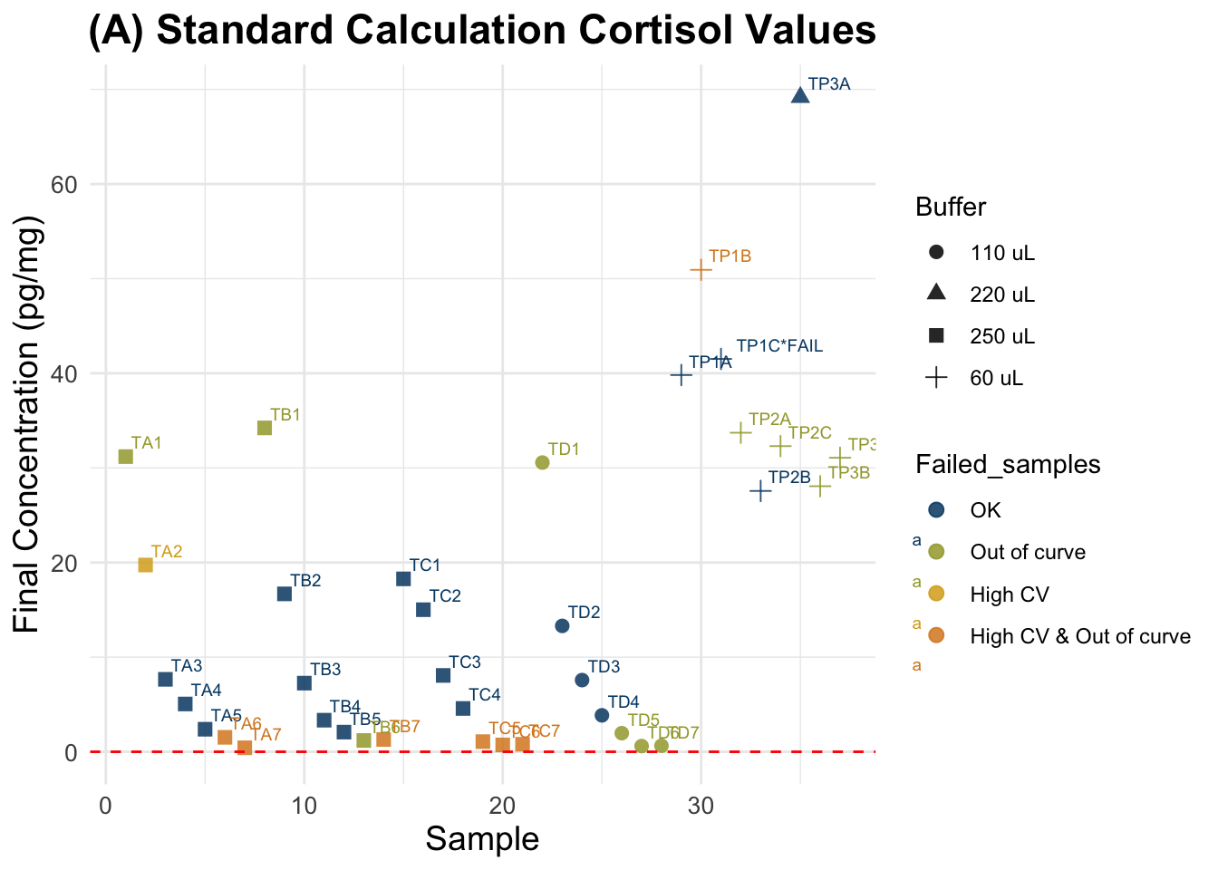
(A) Standard Calculation
Final cortisol concentrations not accounting for spike. Tags are sample numbers.
Expected results: a straight horizontal line showing that I obtained same cortisol concentration value in the Y axis, across different sample weights.
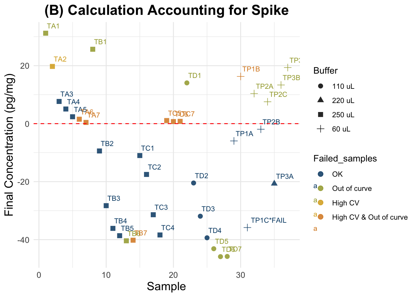
(B) Accounting for Spike
Final cortisol concentrations accounting for Spike as instructed in Nist et al. 2020.
Expected results: lower values than in the previous plot for the spiked samples, but not as low as negative samples (for all of them). Spiked and non-spiked samples should be aligned (same concentration across different weights)
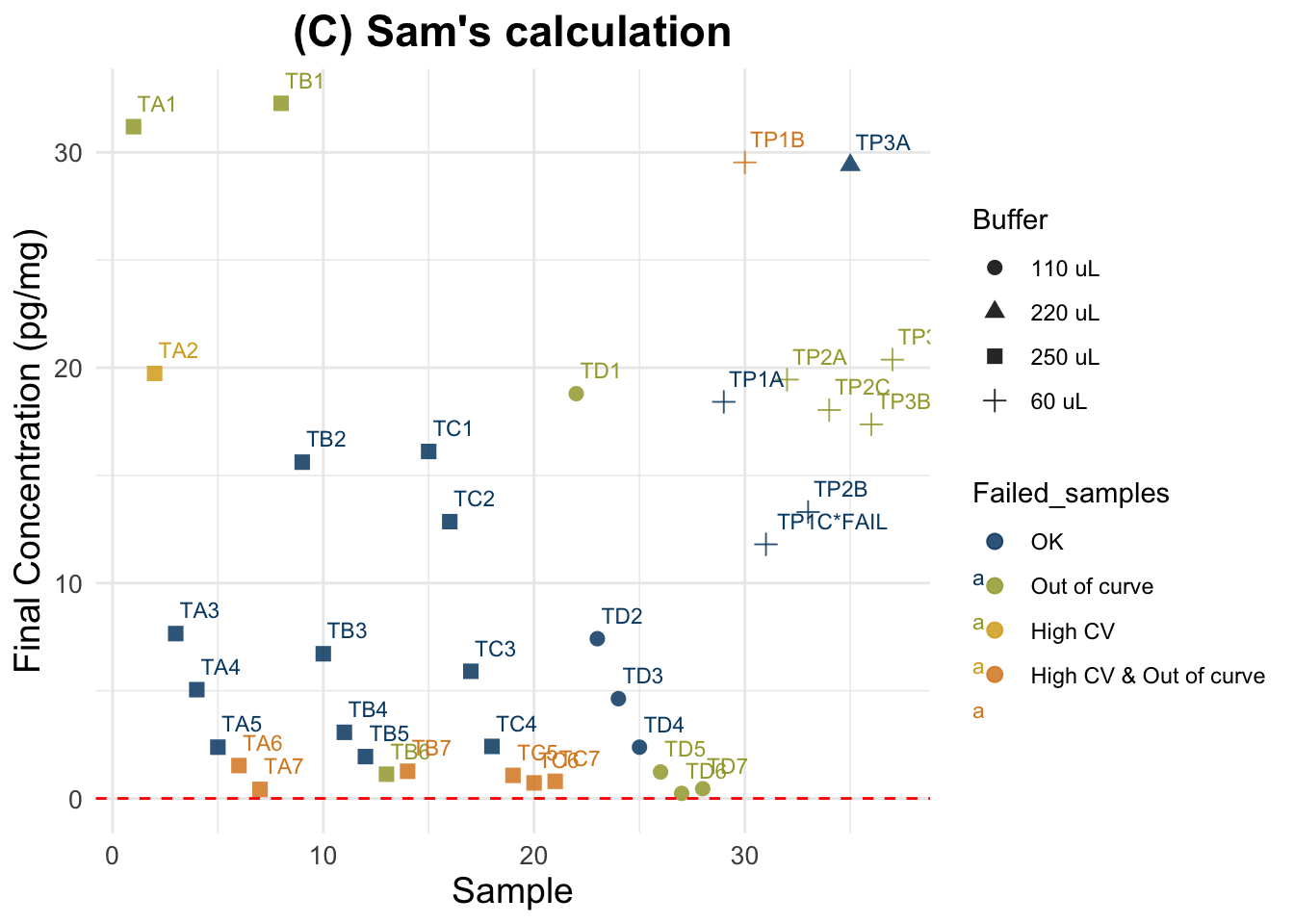
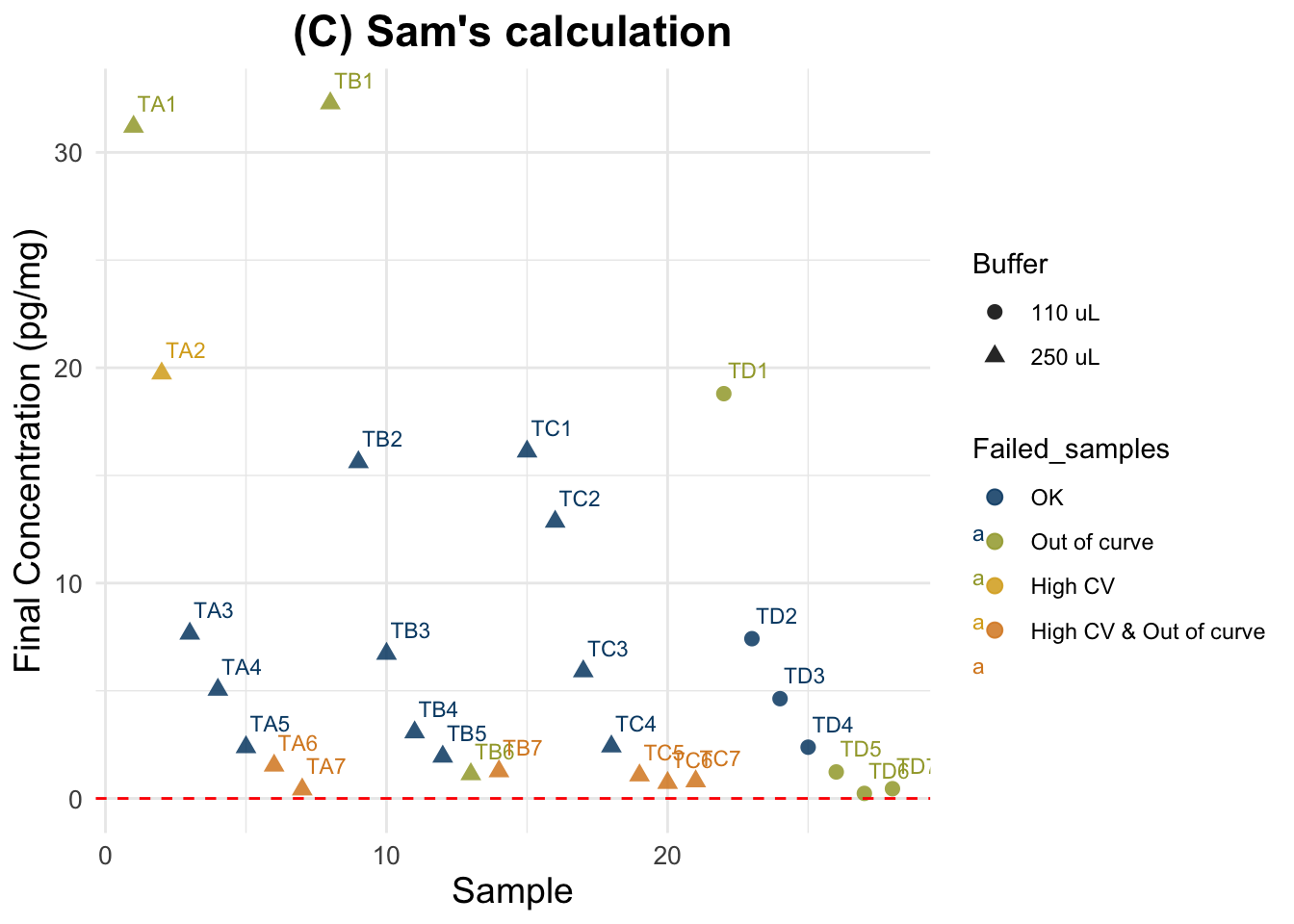
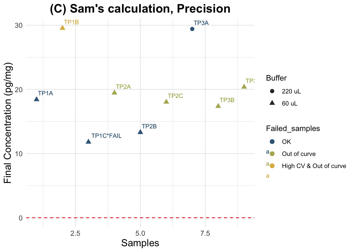
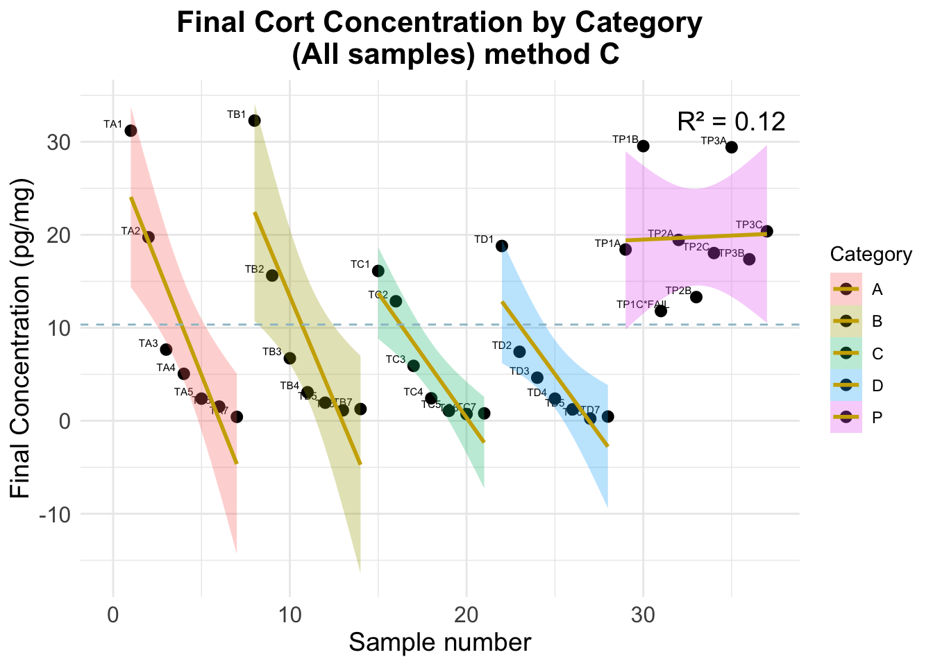
(C) Sam’s calculation
Final cortisol concentration values using new method.
Expected results: one unique horizontal line, regardless of the spiking status and dilution.
Evaluation using C
          1           2           3           4           5           6
 23.7864361  12.3269767   0.2458956  -2.3595098  -5.0284287  -5.8824828
          7           8           9          10          11          12
 -6.9897125  24.8720053   8.2073235  -0.6910931  -4.3396348  -5.4665723
         13          14          15          16          17          18
 -6.2837077  -6.1469421   8.7032848   5.4440255  -1.5041226  -4.9930115
         19          20          21          22          23          24
 -6.3391394  -6.6873617  -6.6132135   5.7631276  -5.6154558  -8.4007474
         25          26          27          28          29          30
-10.6543266 -11.8042162 -12.8005343 -12.5818967   2.7578472  13.8778472
         31          32          33          34          35          36
 -3.8578935   4.3547446  -1.7963665   2.9414113  14.8799378   2.8344198
         37
  5.8410864
8 9 10 11 12 13 14
24.561297 7.896615 -1.001802 -4.650343 -5.777281 -6.594416 -6.457651
15 16 17 18 22 23 24
8.392576 5.133317 -1.814831 -5.303720 5.703641 -5.674942 -8.460234
25 26 27 28 29 30 31
-10.713813 -11.863702 -12.860021 -12.641383 2.815598 13.935598 -3.800143
32 33 34 35 36 37
4.387373 -1.763738 2.974040 14.887444 2.841926 5.848593 1 2 3 4 5 6 7
24.1404901 12.6810307 0.5999496 -2.0054558 -4.6743747 -5.5284288 -6.6356585
19 20 21
-5.9850854 -6.3333077 -6.2591595 Warning: Removed 15 rows containing missing values or values outside the scale range
(`geom_smooth()`).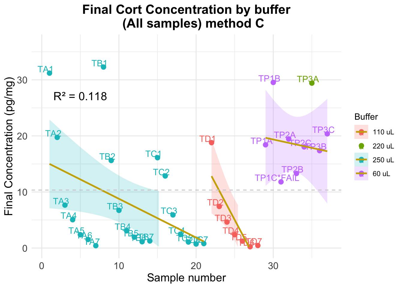
| Version | Author | Date |
|---|---|---|
| dd200fc | Paloma | 2025-04-23 |
| Version | Author | Date |
|---|---|---|
| dd200fc | Paloma | 2025-04-23 |
Optimal dilution (using method C results)
Error using spiked samples only
Mean Absolute Error (MAE) ALL: 7.361 Standard Deviation of Residuals ALL: 9.123 Error using non-spiked samples only
Mean Absolute Error (MAE) ALL: 7.484 Standard Deviation of Residuals ALL: 10.325 Error using all samples
Mean Absolute Error (MAE) ALL: 7.397 Standard Deviation of Residuals ALL: 9.318
sessionInfo()R version 4.5.0 (2025-04-11)
Platform: aarch64-apple-darwin20
Running under: macOS Sequoia 15.4.1
Matrix products: default
BLAS: /Library/Frameworks/R.framework/Versions/4.5-arm64/Resources/lib/libRblas.0.dylib
LAPACK: /Library/Frameworks/R.framework/Versions/4.5-arm64/Resources/lib/libRlapack.dylib; LAPACK version 3.12.1
locale:
[1] en_US.UTF-8/en_US.UTF-8/en_US.UTF-8/C/en_US.UTF-8/en_US.UTF-8
time zone: America/Detroit
tzcode source: internal
attached base packages:
[1] stats graphics grDevices utils datasets methods base
other attached packages:
[1] dplyr_1.1.4 paletteer_1.6.0 broom_1.0.8 ggplot2_3.5.2
[5] knitr_1.50
loaded via a namespace (and not attached):
[1] sass_0.4.10 generics_0.1.3 tidyr_1.3.1 prismatic_1.1.2
[5] lattice_0.22-6 stringi_1.8.7 digest_0.6.37 magrittr_2.0.3
[9] evaluate_1.0.3 grid_4.5.0 fastmap_1.2.0 Matrix_1.7-3
[13] rprojroot_2.0.4 workflowr_1.7.1 jsonlite_2.0.0 whisker_0.4.1
[17] backports_1.5.0 rematch2_2.1.2 promises_1.3.2 mgcv_1.9-1
[21] purrr_1.0.4 scales_1.3.0 jquerylib_0.1.4 cli_3.6.4
[25] rlang_1.1.6 splines_4.5.0 munsell_0.5.1 withr_3.0.2
[29] cachem_1.1.0 yaml_2.3.10 tools_4.5.0 colorspace_2.1-1
[33] httpuv_1.6.16 vctrs_0.6.5 R6_2.6.1 lifecycle_1.0.4
[37] git2r_0.36.2 stringr_1.5.1 fs_1.6.6 pkgconfig_2.0.3
[41] pillar_1.10.2 bslib_0.9.0 later_1.4.2 gtable_0.3.6
[45] glue_1.8.0 Rcpp_1.0.14 xfun_0.52 tibble_3.2.1
[49] tidyselect_1.2.1 rstudioapi_0.17.1 farver_2.1.2 nlme_3.1-168
[53] htmltools_0.5.8.1 rmarkdown_2.29 labeling_0.4.3 compiler_4.5.0