Last updated: 2021-03-24
Checks: 5 1
Knit directory:
thesis/analysis/
This reproducible R Markdown analysis was created with workflowr (version 1.6.2). The Checks tab describes the reproducibility checks that were applied when the results were created. The Past versions tab lists the development history.
Great job! The global environment was empty. Objects defined in the global environment can affect the analysis in your R Markdown file in unknown ways. For reproduciblity it’s best to always run the code in an empty environment.
The command set.seed(20210321) was run prior to running the code in the R Markdown file.
Setting a seed ensures that any results that rely on randomness,
e.g. subsampling or permutations, are reproducible.
Great job! Recording the operating system, R version, and package versions is critical for reproducibility.
Nice! There were no cached chunks for this analysis, so you can be confident that you successfully produced the results during this run.
Great job! Using relative paths to the files within your workflowr project makes it easier to run your code on other machines.
Tracking code development and connecting the code version to the results is
critical for reproducibility. To start using Git, open the Terminal and type
git init in your project directory.
This project is not being versioned with Git. To obtain the full
reproducibility benefits of using workflowr, please see
?wflow_start.
1 Appendix
var_iter = c("**cb**", "**sb**", "**ns**", "**os**")
unit_iter = c("*adm*", "*bas*")
combi = expand.grid(unit_iter, var_iter)
names_unit = combi$Var1
names_var = combi$Var2
Density Plots of Predicted Conflict Probability
files <- list.files("../output/acc/", pattern = ".rds", full.names = T)

data <- lapply(files, function(x){
  out = vars_detect(x)
  tmp = readRDS(x)

  thres_df = readRDS(
    paste0(
      "../output/test-results/test-results-",
      paste(out$type, out$unit, out$var, sep = "-"),
      ".rds")
  )
  if(out$var == "all"){
    for(i in 1:length(tmp)){
      tmp[[i]]$df$var = "cb"
      out$var = "cb"
    }
  }
  thres_df %>%
    filter(name == "f2", month == 0) %>%
    filter(score == max(score, na.rm = T)) %>%
    pull(rep) -> rep

  thres_df %>%
    filter(name == "threshold", rep == !!rep) %>%
    pull(score) -> threshold

  list(unit = out$unit, type = out$type, var = out$var, thres = threshold, df = tmp[[rep]]$df)
})

units <- unlist(lapply(data, `[[`, 1))
types <- unlist(lapply(data, `[[`, 2))
vars <- unlist(lapply(data, `[[`, 3))
dfs <-  lapply(data, `[[`, 4)


var_iter = c("cb", "sb", "ns", "os")
unit_iter = c("states", "basins")
type_iter = c("baseline", "structural", "environmental")


for(var in var_iter){
  tmp1 = data[vars == var]
  for(unit in unit_iter){
    unit_lab = if_else(unit == "states", "adm", "bas")
    units =  unlist(lapply(tmp1, `[[`, 1))
    tmp2 = tmp1[units == unit]
    types =  unlist(lapply(tmp2, `[[`, 2))
    thresholds = unlist(lapply(tmp2, `[[`, 4))
    thresholds = data.frame(type = factor(types,
                                          levels = c("baseline", "structural", "environmental"),
                                          labels = c("CH", "SV", "EV")),
                            thresholds = thresholds)

    df = do.call(rbind, lapply(tmp2, `[[`, 5))
    opts_current$set(label = paste("dens", unit,var, sep = "-")) # setting label
    df %>%
      mutate(type = factor(type,
                           levels = c("baseline", "structural", "environmental"),
                           labels = c("CH", "SV", "EV")),
             unit = factor(unit,
                           levels = c("states", "basins"),
                           labels = c("adm", "bas")),
             obsv = factor(obsv,
                           levels = c("peace", "conflict"),
                           labels = c("Peace", "Conflict"))) %>%
      ggplot() +
      geom_density(aes(x=pred, fill = obsv), alpha = .4) +
      geom_vline(data = thresholds, aes(xintercept=thresholds), linetype=2) +
      xlim(0,1) +
      labs(fill = "", x = "Predicted Probability", y = "Density",
           subtitle = paste0("Unit: *", unit_lab, "*      Variable: **",var,"**")) +
      scale_fill_brewer(palette="Dark2") +
      facet_wrap(~type, scales = "free_y")+
      my_theme +
      theme(plot.subtitle =  element_markdown(size = 10)) -> plt_out
    print(plt_out)
  }
}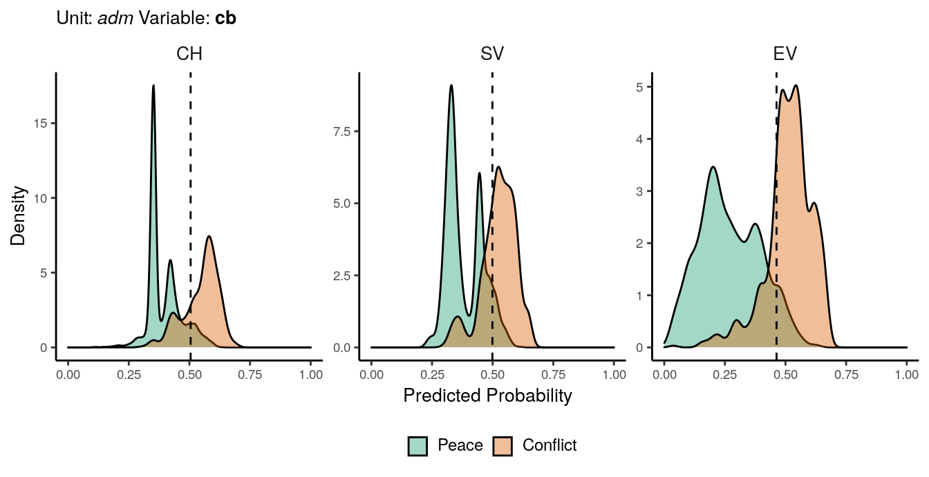
Figure 1.1: Predicted probability of cb conflicts for adm districts. Note that in order to increase visibility the scale on the y-axis differs from one facet to another.
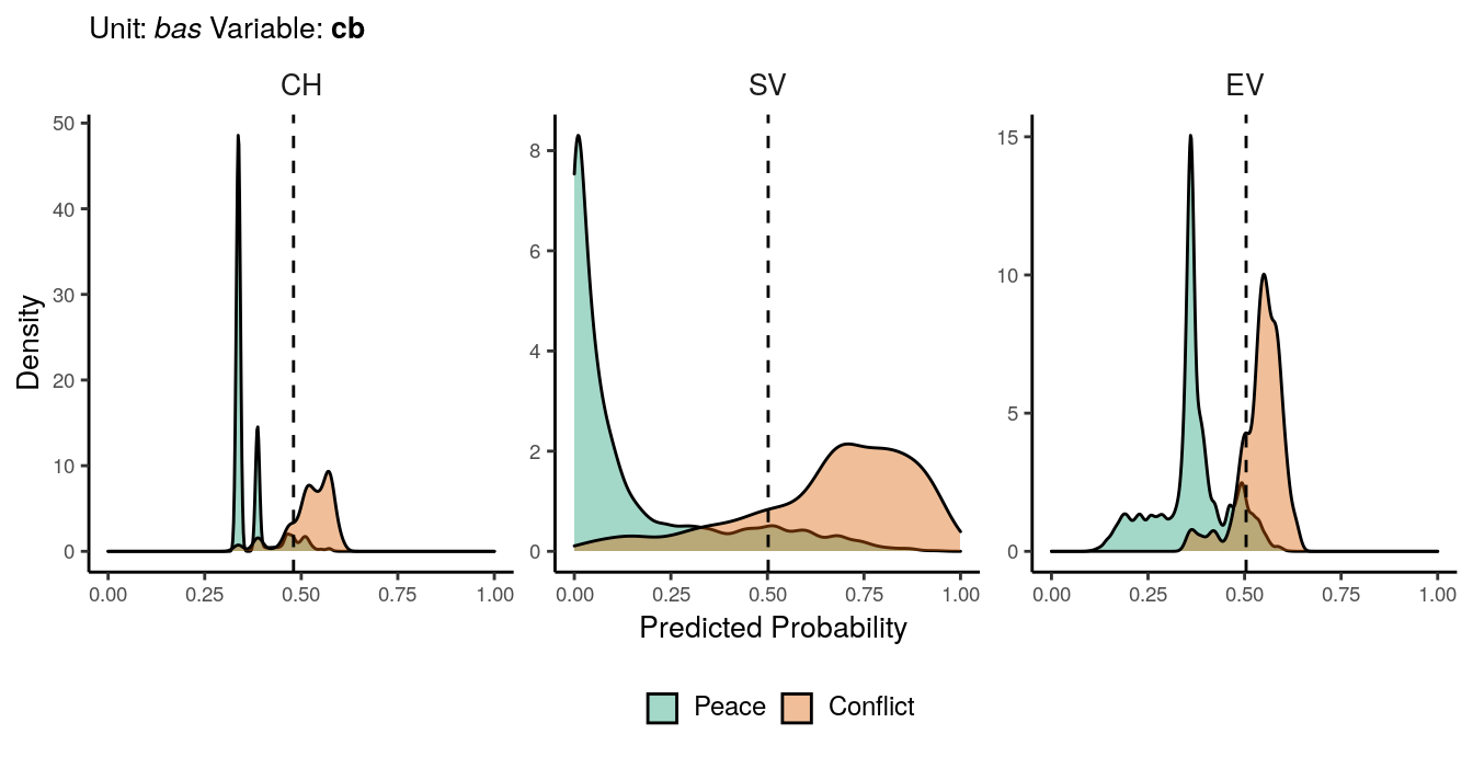
Figure 1.2: Predicted probability of cb conflicts for bas districts. Note that in order to increase visibility the scale on the y-axis differs from one facet to another.
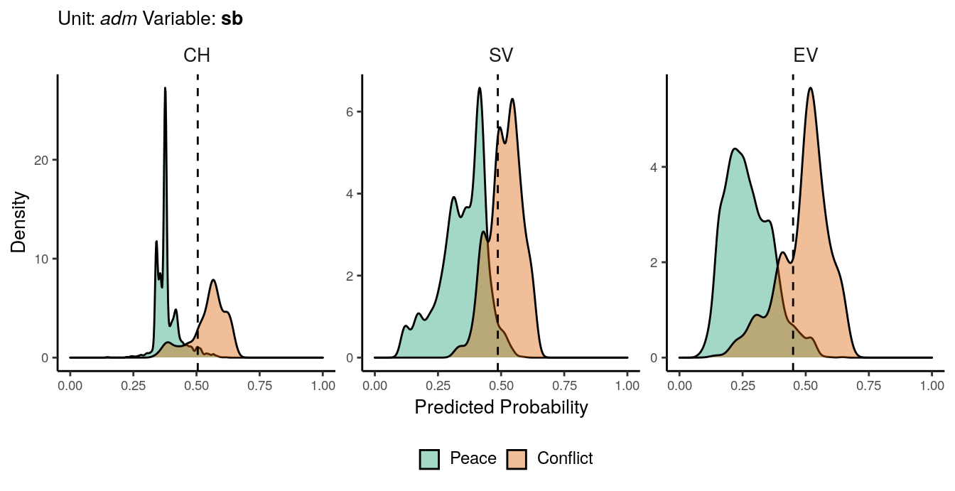
Figure 1.3: Predicted probability of sb conflicts for adm districts. Note that in order to increase visibility the scale on the y-axis differs from one facet to another.
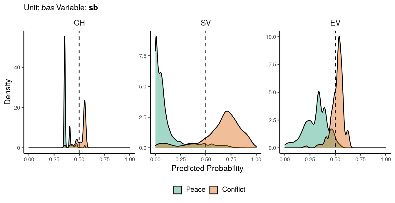
Figure 1.4: Predicted probability of sb conflicts for bas districts. Note that in order to increase visibility the scale on the y-axis differs from one facet to another.
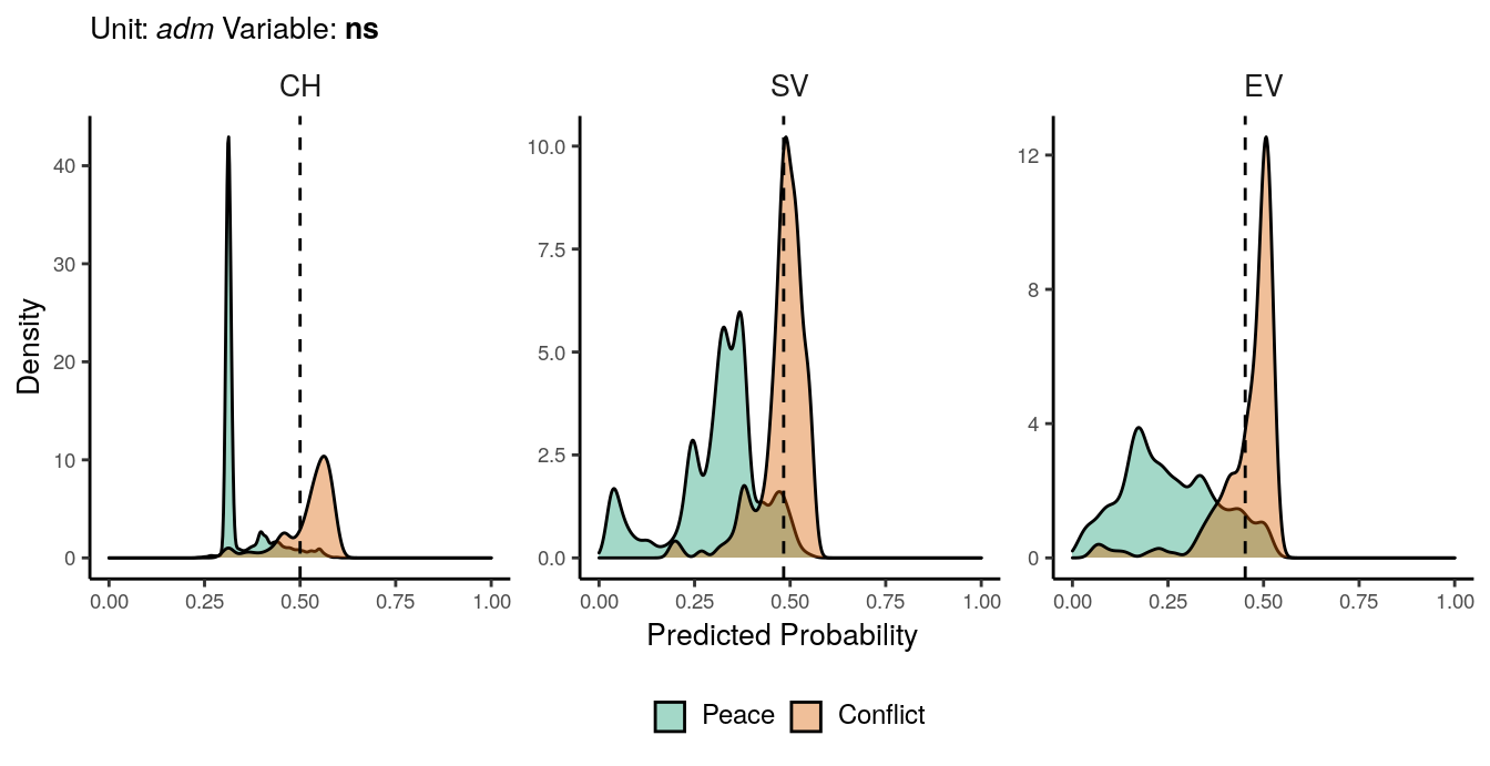
Figure 1.5: Predicted probability of ns conflicts for adm districts. Note that in order to increase visibility the scale on the y-axis differs from one facet to another.
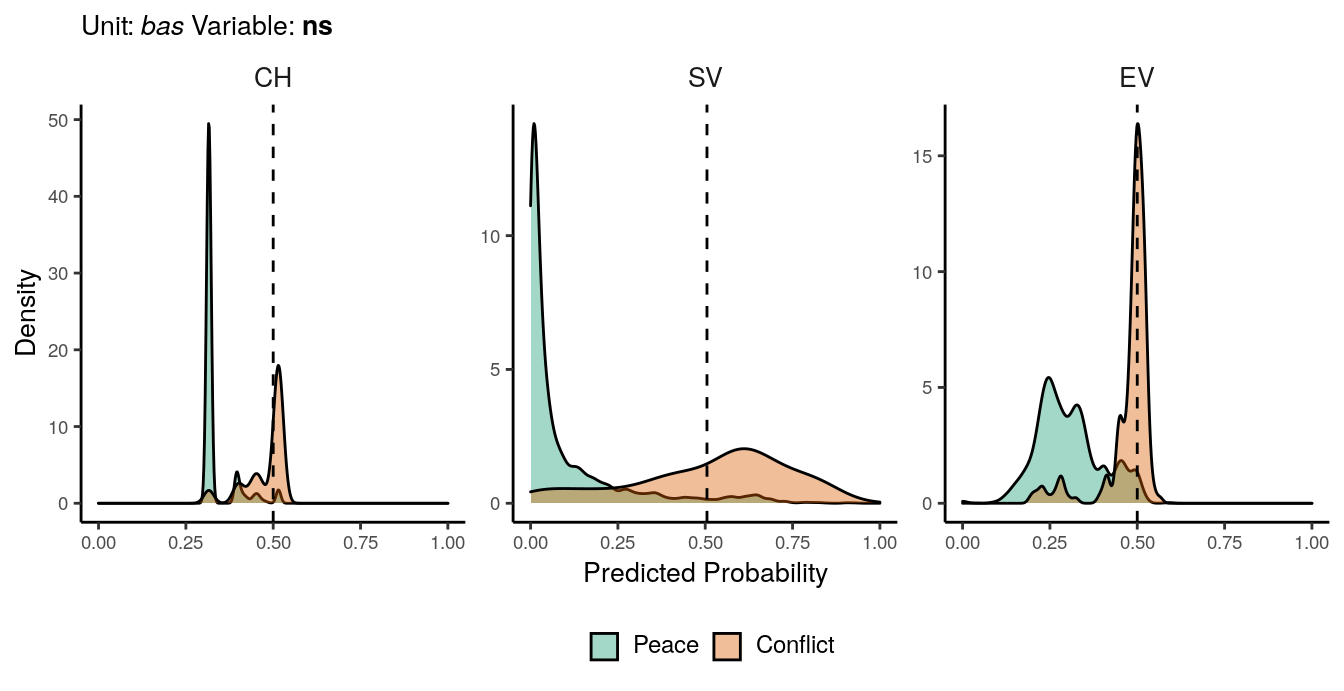
Figure 1.6: Predicted probability of ns conflicts for bas districts. Note that in order to increase visibility the scale on the y-axis differs from one facet to another.
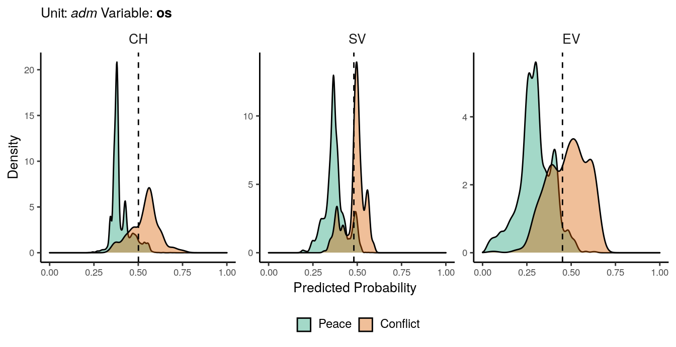
Figure 1.7: Predicted probability of os conflicts for adm districts. Note that in order to increase visibility the scale on the y-axis differs from one facet to another.
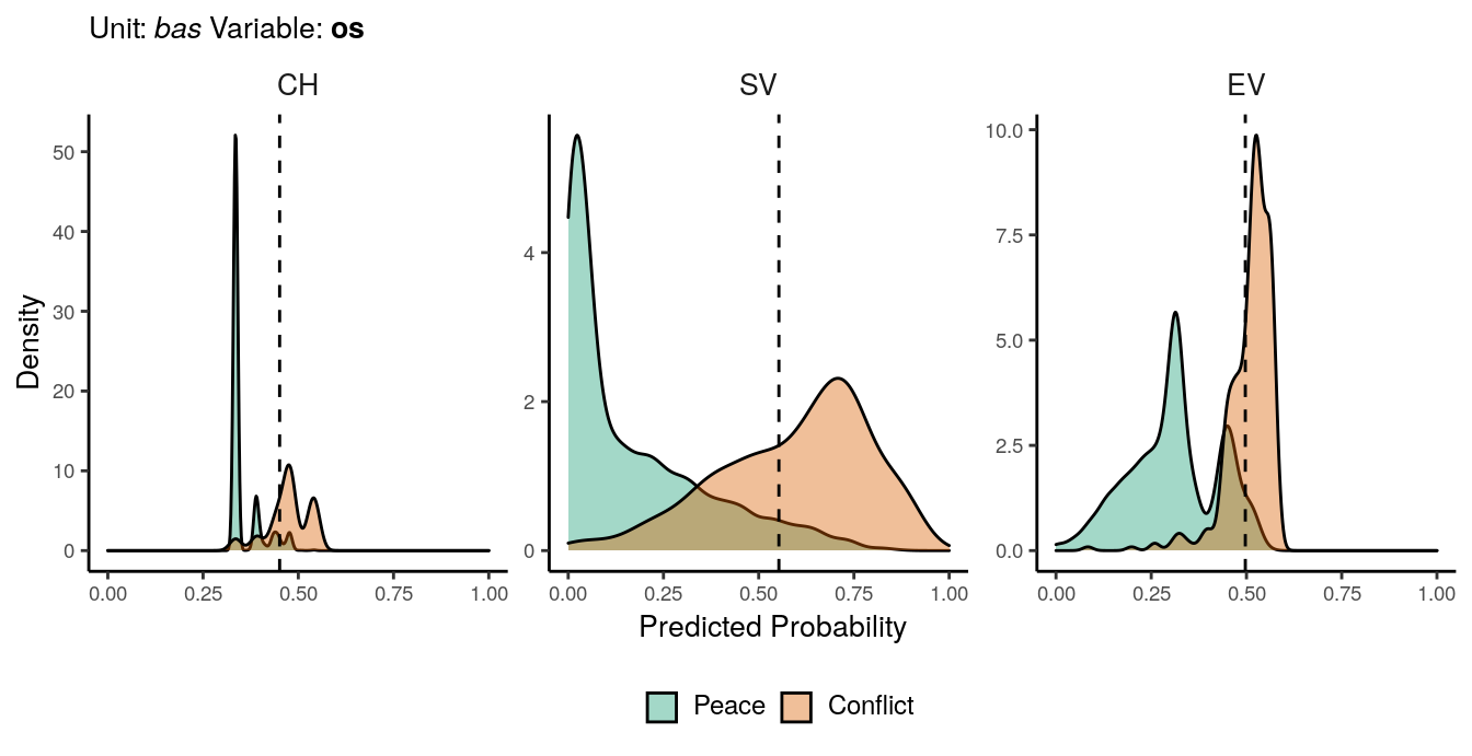
Figure 1.8: Predicted probability of os conflicts for bas districts. Note that in order to increase visibility the scale on the y-axis differs from one facet to another.
Additional Global Performance Metrics
#files <- list.files("../output/acc/", pattern = ".rds", full.names = T)
files <- list.files("../output/test-results/", pattern = "test-results", full.names = T)
# files <- files[-grep("test-results-regression-basins", files)]
acc_data <- lapply(files, function(x){
  out <- vars_detect(x)
  tmp = readRDS(x)
  tmp %>%
    filter(month == 0) %>%
    group_by(name) %>%
    summarise(mean = mean(score, na.rm = T),
              median = median(score, na.rm = TRUE),
              sd = sd(score, na.rm = T),
              type = out$type,
              unit = out$unit,
              var = out$var) %>%
    ungroup()
})
acc_data = do.call(rbind, acc_data)

acc_data %<>%
  mutate(var = factor(var,
                      levels = c("all", "sb", "ns", "os"),
                      labels = c("cb", "sb", "ns", "os")),
         type = factor(type,
                       labels = c("LR", "CH", "SV", "EV"),
                       levels = c("regression", "baseline", "structural", "environmental")),
         unit = if_else(unit == "basins", "bas", "adm"),
         unit = factor(unit, levels = c("adm", "bas"), labels = c("adm", "bas")))

pd <- position_dodge(0.1)
score = "median"
labs.unit = c("_adm_", "_bas_")
names(labs.unit) = c("adm", "bas")
labs.name = c("", "")
names(labs.name) = c("AUC", "AUC")
plt_auc = acc_data %>%
dplyr::filter(name == "auc") %>%
dplyr::select(type, unit, var, name, score = !!score, sd) %>%
ggplot(aes(color=var, x=type, shape=var)) +
geom_point(aes(y=score), position = position_dodge2(width = .5)) +
geom_errorbar(aes(ymin=score-sd, ymax=score+sd, x=type), width=.5, position = position_dodge2(width = .5)) +
scale_color_brewer(palette = "Dark2") +
labs(x="", y = "AUC", color = "Conflict Class", shape = "Conflict Class") +
ylim(0,1) +
facet_wrap(~unit+name, labeller = labeller(unit = labs.unit, name = labs.name)) +
guides(color=guide_legend(ncol=4)) +
my_theme
plt_spec = acc_data %>%
filter(name == "specificity") %>%
dplyr::select(type, unit, var, name, score = !!score, sd) %>%
ggplot(aes(color=var, x=type, shape=var)) +
geom_point(aes(y=score), position = position_dodge2(width = .5)) +
geom_errorbar(aes(ymin=score-sd, ymax=score+sd, x=type), width=.5, position = position_dodge2(width = .5)) +
scale_color_brewer(palette = "Dark2") +
labs(x="Model type", y = "Specificity", color = "Conflict Class", shape = "Conflict Class") +
ylim(0,1) +
facet_wrap(~unit+name, labeller = labeller(unit = labs.unit, name = labs.name)) +
guides(color=guide_legend(ncol=4)) +
my_theme
if(knitr::is_latex_output()){
ggarrange(plt_auc, plt_spec, ncol = 1, common.legend = T, legend = "bottom")
} else {
require(plotly)
subplot(plt_auc, plt_spec, nrows = 2) %>%
layout(legend = list(orientation = "h",
xanchor = "center",
x = 0.5, y = -.1))
}Figure 1.9: Global performance of the AUC metric (top) and pecificity (bottom).
Additional Temporal Performance Metrics
#files <- list.files("../output/acc/", pattern = ".rds", full.names = T)
files <- list.files("../output/test-results/", pattern = "test-results", full.names = T)
# files <- files[-grep("test-results-regression-basins", files)]
acc_data <- lapply(files, function(x){
  out <- vars_detect(x)
  tmp = readRDS(x)
  tmp$type = out$type

  tmp %>%
    filter(month != 0)
})
acc_data = do.call(rbind, acc_data)

acc_data %<>%
  mutate(var = factor(var, labels = c("all", "sb", "ns", "os"),
                      levels = c("all", "sb", "ns", "os")),
         type = factor(type,
                       labels = c("LR", "CH", "SV", "EV"),
                       levels = c("regression", "baseline", "structural", "environmental")),
         unit = if_else(unit == "basins", "bas", "adm"),
         unit = factor(unit, levels = c("adm", "bas"), labels = c("adm", "bas")))

labs.unit = c("_adm_", "_bas_")
names(labs.unit) = c("adm", "bas")
labs.var = c("__cb__", "__sb__", "__ns__", "__os__")
names(labs.var) = c("all", "sb", "ns", "os")
acc_data %>%
filter(name == "auc") %>%
dplyr::select(name, score, month, var, unit, type) %>%
ggplot(aes(x=month, y=score, color=type, linetype=type))+
stat_smooth(geom='line', alpha=.4, size=.5, se=FALSE, lwd=1)+
facet_grid(unit~var, labeller = labeller(unit = labs.unit, var = labs.var)) +
scale_x_continuous(breaks=c(1:12)) +
ylim(0,1) +
theme_classic() +
scale_color_brewer(palette="Dark2") +
labs(subtitle = "AUC", x = "Prediction window (in months)", y = "Score", color = "Model", linetype = "Model") +
guides(color=guide_legend(ncol=4)) +
my_theme -> plt_out
plot_output(plt_out)Figure 1.10: Time dependent performance of the AUC metric.
acc_data %>%
  filter(name == "specificity") %>%
  dplyr::select(name, score, month, var, unit, type) %>%
  ggplot(aes(x=month, y=score, color=type, linetype=type))+
  stat_smooth(geom='line', alpha=.4, size=.5, se=FALSE, lwd=1)+
  facet_grid(unit~var, labeller = labeller(unit = labs.unit, var = labs.var)) +
  scale_x_continuous(breaks=c(1:12)) +
  ylim(0,1) +
  theme_classic() +
  scale_color_brewer(palette="Dark2") +
  labs(subtitle = "Specificity", x = "Prediction window (in months)", y = "Score", color = "Model", linetype="Model") +
  guides(color=guide_legend(ncol=4)) +
  my_theme -> plt_out
plot_output(plt_out)
Figure 1.11: Time dependent performance of specificity.
ROC Curves
files <- list.files("../output/acc/", pattern = ".rds", full.names = T)

auc_data <- lapply(files, function(x){
  out <- vars_detect(x)
  tmp = readRDS(x)

  df_auc <- lapply(1:length(tmp), function(i){
    rep = tmp[[i]]$rep
    FPR = tmp[[i]]$auc$curve[,1]
    recall = tmp[[i]]$auc$curve[,2]
    FPR = FPR[ c(rep(FALSE, 3), TRUE)] # reduce to every 4th entry to reduce file size
    recall = recall[ c(rep(FALSE, 3), TRUE)] # reduce to every 4th entry to reduce file size

    auc <- tibble(type = out$type,
                  unit = out$unit,
                  var = out$var,
                  rep = rep,
                  FPR = FPR,
                  recall = recall)
  })
  df_auc = do.call(rbind, df_auc)
})

auc_data <- do.call(rbind, auc_data)

auc_data %<>%
  mutate(var = factor(var,
                      labels = c("__cb__", "__sb__", "__ns__", "__os__"),
                      levels = c("all", "sb", "ns", "os")),
         type = factor(type,
                       labels = c("CH", "SV", "EV"),
                       levels = c("baseline", "structural", "environmental")),
         unit = factor(unit, levels = c("states", "basins"), labels = c("adm", "bas")))
auc_data %>%
filter(unit == "adm") %>%
mutate(group = paste(type,var,rep,sep="-")) %>%
ggplot(aes(x=FPR, y=recall,color=type,linetype=type)) +
geom_line(aes(group=group), size=.1, alpha = .5) +
geom_smooth(alpha=1, size=.5, se=FALSE) +
scale_color_manual(values = RColorBrewer::brewer.pal(n=4, name = "Dark2")[2:4]) +
facet_wrap(~var, ncol = 2) +
labs(color = "Model", linetype="Model", y = "Sensitivity", x = "FPR", subtitle = "adm") +
guides(color=guide_legend(override.aes = list(alpha = 1, ncol = 3))) +
my_theme +
theme(
plot.subtitle = element_markdown(size = 10, face = "italic")
) 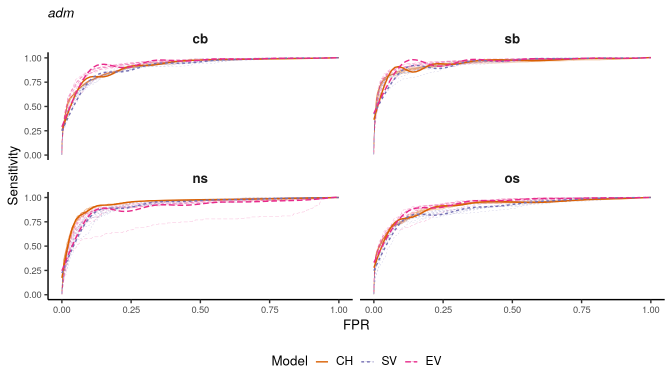
Figure 1.12: ROC curves for adm district models.
auc_data %>%
  filter(unit == "bas") %>%
  mutate(group = paste(type,var,rep,sep="-")) %>%
  ggplot(aes(x=FPR, y=recall,color=type,linetype=type)) +
  geom_line(aes(group=group), size=.1, alpha = .5) +
  geom_smooth(alpha=1, size=.5, se=FALSE) +
  scale_color_manual(values = RColorBrewer::brewer.pal(n=4, name  = "Dark2")[2:4]) +
  facet_wrap(~var, ncol = 2) +
  labs(color = "Model", linetype="Model", y = "Sensitivity", x = "FPR", subtitle = "bas") +
  guides(color=guide_legend(override.aes = list(alpha = 1, ncol = 3))) +
  my_theme +
  theme(
    plot.subtitle =  element_markdown(size = 10, face =  "italic")
  )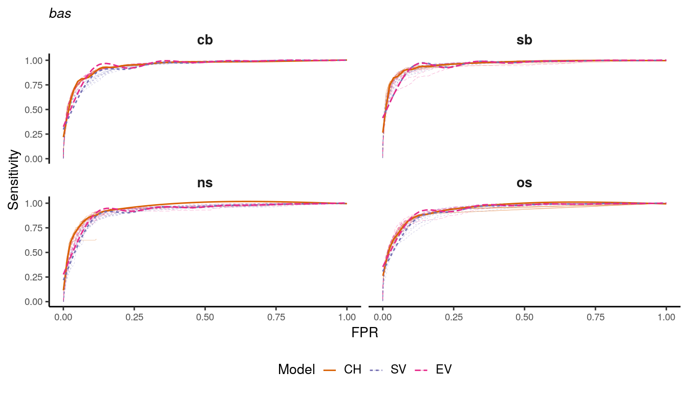
Figure 1.13: ROC curves for bas district models.
adm <- st_read("../data/vector/states_mask.gpkg", quiet = T)
adm <- select(adm, geom)
adm <- st_make_valid(adm)
bas <- st_read("../data/vector/basins_simple.gpkg", quiet = T)
bas <- select(bas, geom)
bas <- st_make_valid(bas)
crs <- st_crs("EPSG:3857")
adm <- st_transform(adm, crs)
adm <- st_simplify(adm, dTolerance = 1500, preserveTopology = T)
bas <- st_transform(bas, crs)
bas <- st_simplify(bas, dTolerance = 1000, preserveTopology = T)


files = list.files("../output/test-results/", pattern ="cnfrisk", full.names = T)

map_data = lapply(files, function(x){
  out = vars_detect(x)
  tmp = st_read(x, quiet = T)
  tmp = st_drop_geometry(tmp)
  tmp$unit = out$unit
  tmp$type = out$type
  tmp$var = out$var
  tmp %<>%
    select(unit,type,var,mean,obsv)
  if(out$unit == "basins") {
    st_as_sf(bind_cols(bas, tmp))
  } else {
    st_as_sf(bind_cols(adm, tmp))
  }
})

map_data = do.call(rbind, map_data)
map_data %>%
filter(unit == "states", var == "sb") -> plt_data
breaks = seq(0,1,0.1)
plt_data %>%
filter(type == "baseline") %>%
dplyr::select(obsv) %>%
mutate(obsv = ifelse(obsv > 0, obsv, NA)) -> obsv_data
obsv_data %>%
tm_shape() +
tm_polygons("obsv",
palette = "PuBu",
lwd=.01,
border.col = "grey90",
breaks = 0:12,
style = "fixed",
title = "Conflict Months",
showNA = FALSE,
legend.hist = TRUE,
labels = as.character(1:12)) +
tm_legend(stack = "horizontal") +
tm_layout(title = "Observation",
title.position = c("right", "top"),
title.size = 0.7,
legend.title.size = 0.7,
legend.text.size = 0.45,
legend.position = c("left", "bottom"),
legend.outside.position = "bottom",
legend.bg.color = "white",
legend.bg.alpha = 0,
legend.outside = TRUE,
legend.hist.width = 1,
legend.hist.height = .8,
legend.hist.size = .5) -> map_obsv
plt_data %>%
filter(type == "baseline") %>%
tm_shape() +
tm_polygons("mean",
palette = "PuBu",
lwd=.01,
border.col = "grey90",
title = "Probability of conflict",
breaks = breaks,
style = "fixed",
legend.hist = TRUE) +
tm_legend(stack = "horizontal") +
tm_layout(title = "Conflict History (CH)",
title.position = c("right", "top"),
title.size = 0.7,
legend.title.size = 0.7,
legend.text.size = 0.45,
legend.position = c("left", "bottom"),
legend.outside.position = "bottom",
legend.bg.color = "white",
legend.bg.alpha = 0,
legend.outside = TRUE,
legend.hist.width = 1,
legend.hist.height = .8,
legend.hist.size = .5) -> map_bas
plt_data %>%
filter(type == "structural") %>%
tm_shape() +
tm_polygons("mean",
palette = "PuBu",
lwd=.01,
border.col = "grey90",
title = "Probability of conflict",
breaks = breaks,
style = "fixed",
legend.hist = TRUE) +
tm_legend(stack = "horizontal") +
tm_layout(title = "Structural Variables (SV)",
title.position = c("right", "top"),
title.size = 0.7,
legend.title.size = 0.7,
legend.text.size = 0.45,
legend.position = c("left", "bottom"),
legend.outside.position = "bottom",
legend.bg.color = "white",
legend.bg.alpha = 0,
legend.outside = TRUE,
legend.hist.width = 1,
legend.hist.height = .8,
legend.hist.size = .5) -> map_str
plt_data %>%
filter(type == "environmental") %>%
tm_shape() +
tm_polygons("mean",
palette = "PuBu",
lwd=.01,
border.col = "grey90",
title = "Probability of conflict",
breaks = breaks,
style = "fixed",
legend.hist = TRUE) +
tm_legend(stack = "horizontal") +
tm_layout(title = "Environmental Variables (EV)",
title.position = c("right", "top"),
title.size = 0.7,
legend.title.size = 0.7,
legend.text.size = 0.45,
legend.position = c("left", "bottom"),
legend.outside.position = "bottom",
legend.bg.color = "white",
legend.bg.alpha = 0,
legend.outside = TRUE,
legend.hist.width = 1,
legend.hist.height = .8,
legend.hist.size = .5) -> map_env
tmap_arrange(map_obsv, map_bas, map_str, map_env, ncol = 2)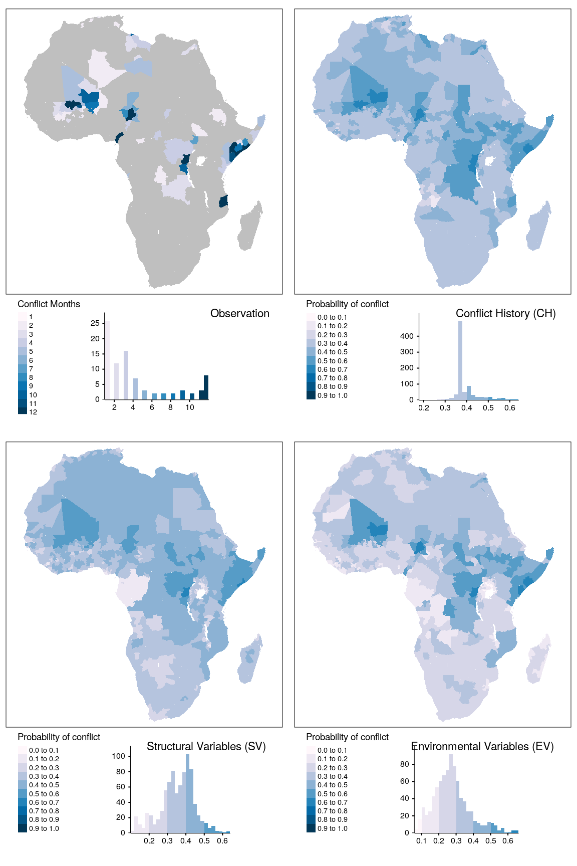
Figure 1.14: Spatial prediction of conflict class sb for adm districts.
map_data %>%
  filter(unit == "states", var == "ns") -> plt_data

breaks = seq(0,1,0.1)

plt_data %>%
  filter(type == "baseline") %>%
  dplyr::select(obsv) %>%
  mutate(obsv = ifelse(obsv > 0, obsv, NA)) -> obsv_data

obsv_data %>%
  tm_shape() +
  tm_polygons("obsv",
              palette = "PuBu",
              lwd=.01,
              border.col = "grey90",
              breaks = 0:12,
              style = "fixed",
              title = "Conflict Months",
              showNA = FALSE,
              legend.hist = TRUE,
              labels = as.character(1:12)) +
  tm_legend(stack = "horizontal") +
  tm_layout(title = "Observation",
            title.position = c("right", "top"),
            title.size = 0.7,
            legend.title.size = 0.7,
            legend.text.size = 0.45,
            legend.position = c("left", "bottom"),
            legend.outside.position = "bottom",
            legend.bg.color = "white",
            legend.bg.alpha = 0,
            legend.outside = TRUE,
            legend.hist.width = 1,
            legend.hist.height = .8,
            legend.hist.size = .5)   -> map_obsv

plt_data %>%
  filter(type == "baseline") %>%
  tm_shape() +
  tm_polygons("mean",
              palette = "PuBu",
              lwd=.01,
              border.col = "grey90",
              title = "Probability of conflict",
              breaks = breaks,
              style = "fixed",
              legend.hist = TRUE) +
  tm_legend(stack = "horizontal") +
  tm_layout(title = "Conflict History (CH)",
            title.position = c("right", "top"),
            title.size = 0.7,
            legend.title.size = 0.7,
            legend.text.size = 0.45,
            legend.position = c("left", "bottom"),
            legend.outside.position = "bottom",
            legend.bg.color = "white",
            legend.bg.alpha = 0,
            legend.outside = TRUE,
            legend.hist.width = 1,
            legend.hist.height = .8,
            legend.hist.size = .5)   -> map_bas

plt_data %>%
  filter(type == "structural") %>%
  tm_shape() +
  tm_polygons("mean",
              palette = "PuBu",
              lwd=.01,
              border.col = "grey90",
              title = "Probability of conflict",
              breaks = breaks,
              style = "fixed",
              legend.hist = TRUE)  +
  tm_legend(stack = "horizontal") +
  tm_layout(title = "Structural Variables (SV)",
            title.position = c("right", "top"),
            title.size = 0.7,
            legend.title.size = 0.7,
            legend.text.size = 0.45,
            legend.position = c("left", "bottom"),
            legend.outside.position = "bottom",
            legend.bg.color = "white",
            legend.bg.alpha = 0,
            legend.outside = TRUE,
            legend.hist.width = 1,
            legend.hist.height = .8,
            legend.hist.size = .5)  -> map_str

plt_data %>%
  filter(type == "environmental") %>%
  tm_shape() +
  tm_polygons("mean",
              palette = "PuBu",
              lwd=.01,
              border.col = "grey90",
              title = "Probability of conflict",
              breaks = breaks,
              style = "fixed",
              legend.hist = TRUE)  +
  tm_legend(stack = "horizontal") +
  tm_layout(title = "Environmental Variables (EV)",
            title.position = c("right", "top"),
            title.size = 0.7,
            legend.title.size = 0.7,
            legend.text.size = 0.45,
            legend.position = c("left", "bottom"),
            legend.outside.position = "bottom",
            legend.bg.color = "white",
            legend.bg.alpha = 0,
            legend.outside = TRUE,
            legend.hist.width = 1,
            legend.hist.height = .8,
            legend.hist.size = .5)  -> map_env

tmap_arrange(map_obsv, map_bas, map_str, map_env, ncol = 2)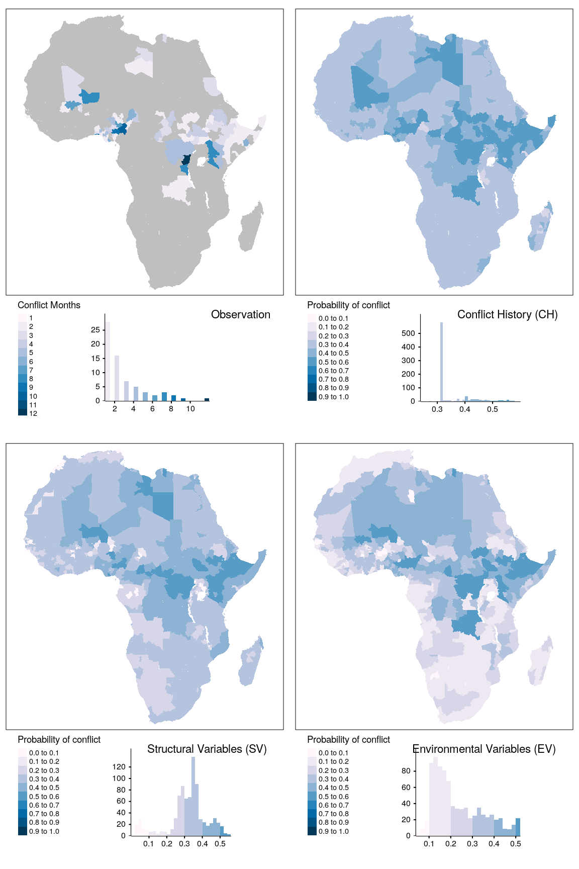
Figure 1.15: Spatial prediction of conflict class ns for adm districts.
map_data %>%
  filter(unit == "states", var == "os") -> plt_data

breaks = seq(0,1,0.1)

plt_data %>%
  filter(type == "baseline") %>%
  dplyr::select(obsv) %>%
  mutate(obsv = ifelse(obsv > 0, obsv, NA)) -> obsv_data

obsv_data %>%
  tm_shape() +
  tm_polygons("obsv",
              palette = "PuBu",
              lwd=.01,
              border.col = "grey90",
              breaks = 0:12,
              style = "fixed",
              title = "Conflict Months",
              showNA = FALSE,
              legend.hist = TRUE,
              labels = as.character(1:12)) +
  tm_legend(stack = "horizontal") +
  tm_layout(title = "Observation",
            title.position = c("right", "top"),
            title.size = 0.7,
            legend.title.size = 0.7,
            legend.text.size = 0.45,
            legend.position = c("left", "bottom"),
            legend.outside.position = "bottom",
            legend.bg.color = "white",
            legend.bg.alpha = 0,
            legend.outside = TRUE,
            legend.hist.width = 1,
            legend.hist.height = .8,
            legend.hist.size = .5)   -> map_obsv

plt_data %>%
  filter(type == "baseline") %>%
  tm_shape() +
  tm_polygons("mean",
              palette = "PuBu",
              lwd=.01,
              border.col = "grey90",
              title = "Probability of conflict",
              breaks = breaks,
              style = "fixed",
              legend.hist = TRUE) +
  tm_legend(stack = "horizontal") +
  tm_layout(title = "Conflict History (CH)",
            title.position = c("right", "top"),
            title.size = 0.7,
            legend.title.size = 0.7,
            legend.text.size = 0.45,
            legend.position = c("left", "bottom"),
            legend.outside.position = "bottom",
            legend.bg.color = "white",
            legend.bg.alpha = 0,
            legend.outside = TRUE,
            legend.hist.width = 1,
            legend.hist.height = .8,
            legend.hist.size = .5)   -> map_bas

plt_data %>%
  filter(type == "structural") %>%
  tm_shape() +
  tm_polygons("mean",
              palette = "PuBu",
              lwd=.01,
              border.col = "grey90",
              title = "Probability of conflict",
              breaks = breaks,
              style = "fixed",
              legend.hist = TRUE)  +
  tm_legend(stack = "horizontal") +
  tm_layout(title = "Structural Variables (SV)",
            title.position = c("right", "top"),
            title.size = 0.7,
            legend.title.size = 0.7,
            legend.text.size = 0.45,
            legend.position = c("left", "bottom"),
            legend.outside.position = "bottom",
            legend.bg.color = "white",
            legend.bg.alpha = 0,
            legend.outside = TRUE,
            legend.hist.width = 1,
            legend.hist.height = .8,
            legend.hist.size = .5)  -> map_str

plt_data %>%
  filter(type == "environmental") %>%
  tm_shape() +
  tm_polygons("mean",
              palette = "PuBu",
              lwd=.01,
              border.col = "grey90",
              title = "Probability of conflict",
              breaks = breaks,
              style = "fixed",
              legend.hist = TRUE)  +
  tm_legend(stack = "horizontal") +
  tm_layout(title = "Environmental Variables (EV)",
            title.position = c("right", "top"),
            title.size = 0.7,
            legend.title.size = 0.7,
            legend.text.size = 0.45,
            legend.position = c("left", "bottom"),
            legend.outside.position = "bottom",
            legend.bg.color = "white",
            legend.bg.alpha = 0,
            legend.outside = TRUE,
            legend.hist.width = 1,
            legend.hist.height = .8,
            legend.hist.size = .5)  -> map_env

tmap_arrange(map_obsv, map_bas, map_str, map_env, ncol = 2)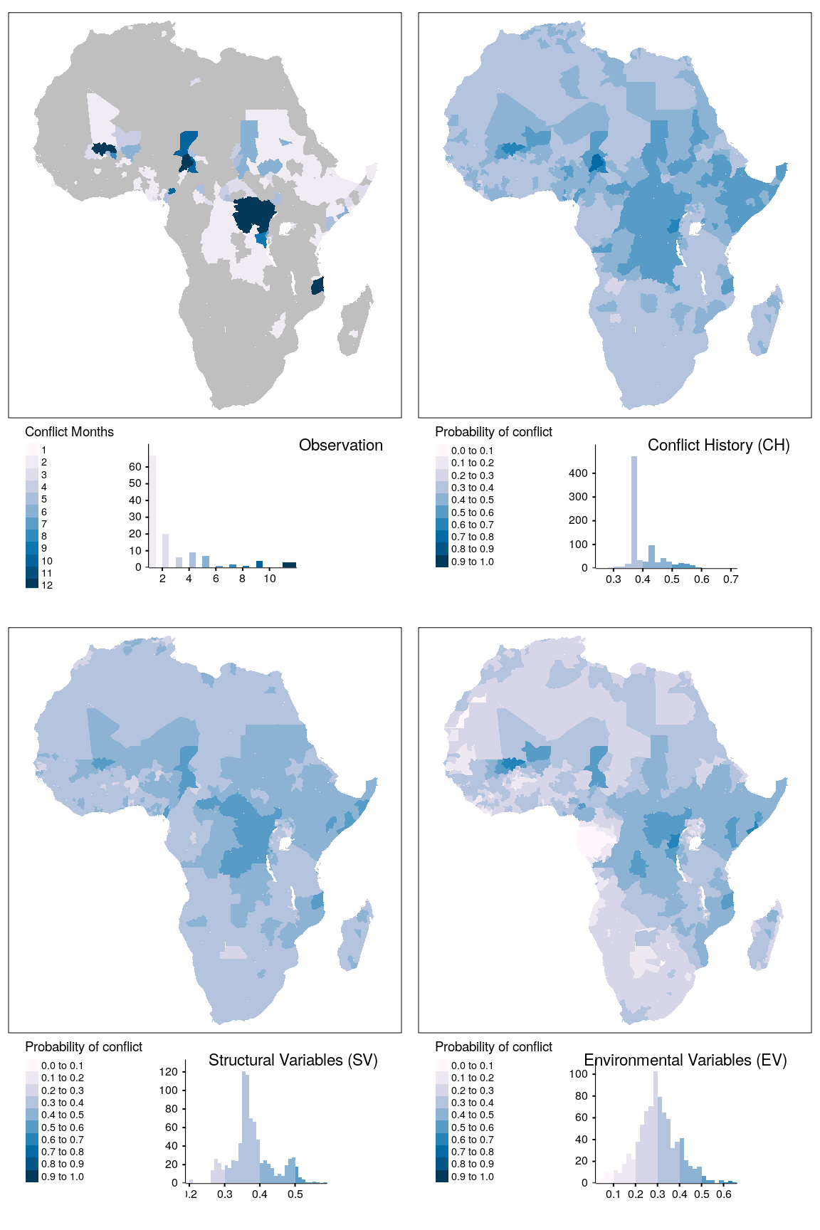
Figure 1.16: Spatial prediction of conflict class os for adm districts.
map_data %>%
  filter(unit == "basins", var == "sb") -> plt_data

breaks = seq(0,1,0.1)

plt_data %>%
  filter(type == "baseline") %>%
  dplyr::select(obsv) %>%
  mutate(obsv = ifelse(obsv > 0, obsv, NA)) -> obsv_data

obsv_data %>%
  tm_shape() +
  tm_polygons("obsv",
              palette = "PuBu",
              lwd=.01,
              border.col = "grey90",
              breaks = 0:12,
              style = "fixed",
              title = "Conflict Months",
              showNA = FALSE,
              legend.hist = TRUE,
              labels = as.character(1:12)) +
  tm_legend(stack = "horizontal") +
  tm_layout(title = "Observation",
            title.position = c("right", "top"),
            title.size = 0.7,
            legend.title.size = 0.7,
            legend.text.size = 0.45,
            legend.position = c("left", "bottom"),
            legend.outside.position = "bottom",
            legend.bg.color = "white",
            legend.bg.alpha = 0,
            legend.outside = TRUE,
            legend.hist.width = 1,
            legend.hist.height = .8,
            legend.hist.size = .5)   -> map_obsv

plt_data %>%
  filter(type == "baseline") %>%
  tm_shape() +
  tm_polygons("mean",
              palette = "PuBu",
              lwd=.01,
              border.col = "grey90",
              title = "Probability of conflict",
              breaks = breaks,
              style = "fixed",
              legend.hist = TRUE) +
  tm_legend(stack = "horizontal") +
  tm_layout(title = "Conflict History (CH)",
            title.position = c("right", "top"),
            title.size = 0.7,
            legend.title.size = 0.7,
            legend.text.size = 0.45,
            legend.position = c("left", "bottom"),
            legend.outside.position = "bottom",
            legend.bg.color = "white",
            legend.bg.alpha = 0,
            legend.outside = TRUE,
            legend.hist.width = 1,
            legend.hist.height = .8,
            legend.hist.size = .5)   -> map_bas

plt_data %>%
  filter(type == "structural") %>%
  tm_shape() +
  tm_polygons("mean",
              palette = "PuBu",
              lwd=.01,
              border.col = "grey90",
              title = "Probability of conflict",
              breaks = breaks,
              style = "fixed",
              legend.hist = TRUE)  +
  tm_legend(stack = "horizontal") +
  tm_layout(title = "Structural Variables (SV)",
            title.position = c("right", "top"),
            title.size = 0.7,
            legend.title.size = 0.7,
            legend.text.size = 0.45,
            legend.position = c("left", "bottom"),
            legend.outside.position = "bottom",
            legend.bg.color = "white",
            legend.bg.alpha = 0,
            legend.outside = TRUE,
            legend.hist.width = 1,
            legend.hist.height = .8,
            legend.hist.size = .5)  -> map_str

plt_data %>%
  filter(type == "environmental") %>%
  tm_shape() +
  tm_polygons("mean",
              palette = "PuBu",
              lwd=.01,
              border.col = "grey90",
              title = "Probability of conflict",
              breaks = breaks,
              style = "fixed",
              legend.hist = TRUE)  +
  tm_legend(stack = "horizontal") +
  tm_layout(title = "Environmental Variables (EV)",
            title.position = c("right", "top"),
            title.size = 0.7,
            legend.title.size = 0.7,
            legend.text.size = 0.45,
            legend.position = c("left", "bottom"),
            legend.outside.position = "bottom",
            legend.bg.color = "white",
            legend.bg.alpha = 0,
            legend.outside = TRUE,
            legend.hist.width = 1,
            legend.hist.height = .8,
            legend.hist.size = .5)  -> map_env

tmap_arrange(map_obsv, map_bas, map_str, map_env, ncol = 2)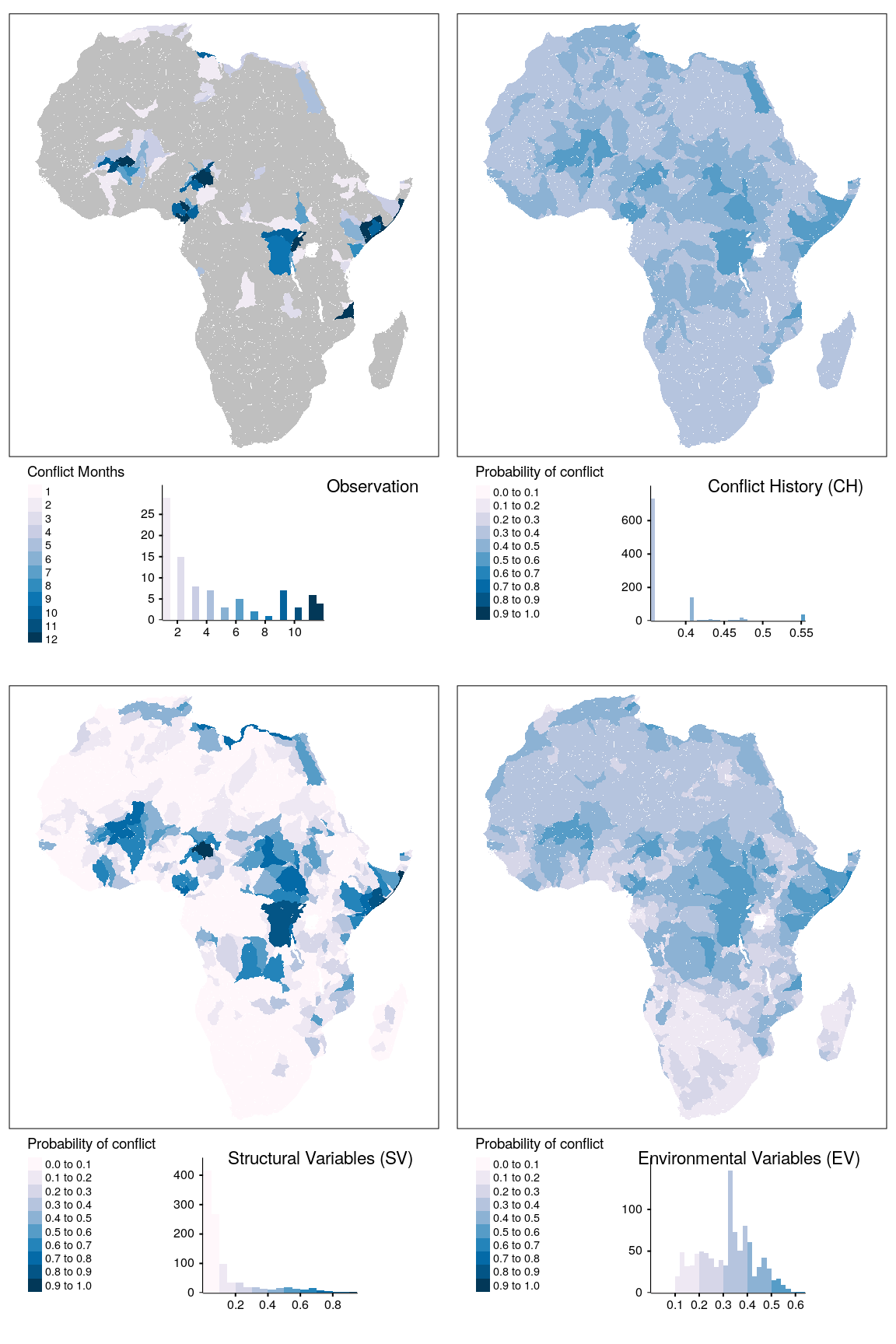
Figure 1.17: Spatial prediction of conflict class sb for bas districts.
map_data %>%
  filter(unit == "basins", var == "ns") -> plt_data

breaks = seq(0,1,0.1)

plt_data %>%
  filter(type == "baseline") %>%
  dplyr::select(obsv) %>%
  mutate(obsv = ifelse(obsv > 0, obsv, NA)) -> obsv_data

obsv_data %>%
  tm_shape() +
  tm_polygons("obsv",
              palette = "PuBu",
              lwd=.01,
              border.col = "grey90",
              breaks = 0:12,
              style = "fixed",
              title = "Conflict Months",
              showNA = FALSE,
              legend.hist = TRUE,
              labels = as.character(1:12)) +
  tm_legend(stack = "horizontal") +
  tm_layout(title = "Observation",
            title.position = c("right", "top"),
            title.size = 0.7,
            legend.title.size = 0.7,
            legend.text.size = 0.45,
            legend.position = c("left", "bottom"),
            legend.outside.position = "bottom",
            legend.bg.color = "white",
            legend.bg.alpha = 0,
            legend.outside = TRUE,
            legend.hist.width = 1,
            legend.hist.height = .8,
            legend.hist.size = .5)   -> map_obsv

plt_data %>%
  filter(type == "baseline") %>%
  tm_shape() +
  tm_polygons("mean",
              palette = "PuBu",
              lwd=.01,
              border.col = "grey90",
              title = "Probability of conflict",
              breaks = breaks,
              style = "fixed",
              legend.hist = TRUE) +
  tm_legend(stack = "horizontal") +
  tm_layout(title = "Conflict History (CH)",
            title.position = c("right", "top"),
            title.size = 0.7,
            legend.title.size = 0.7,
            legend.text.size = 0.45,
            legend.position = c("left", "bottom"),
            legend.outside.position = "bottom",
            legend.bg.color = "white",
            legend.bg.alpha = 0,
            legend.outside = TRUE,
            legend.hist.width = 1,
            legend.hist.height = .8,
            legend.hist.size = .5)   -> map_bas

plt_data %>%
  filter(type == "structural") %>%
  tm_shape() +
  tm_polygons("mean",
              palette = "PuBu",
              lwd=.01,
              border.col = "grey90",
              title = "Probability of conflict",
              breaks = breaks,
              style = "fixed",
              legend.hist = TRUE)  +
  tm_legend(stack = "horizontal") +
  tm_layout(title = "Structural Variables (SV)",
            title.position = c("right", "top"),
            title.size = 0.7,
            legend.title.size = 0.7,
            legend.text.size = 0.45,
            legend.position = c("left", "bottom"),
            legend.outside.position = "bottom",
            legend.bg.color = "white",
            legend.bg.alpha = 0,
            legend.outside = TRUE,
            legend.hist.width = 1,
            legend.hist.height = .8,
            legend.hist.size = .5)  -> map_str

plt_data %>%
  filter(type == "environmental") %>%
  tm_shape() +
  tm_polygons("mean",
              palette = "PuBu",
              lwd=.01,
              border.col = "grey90",
              title = "Probability of conflict",
              breaks = breaks,
              style = "fixed",
              legend.hist = TRUE)  +
  tm_legend(stack = "horizontal") +
  tm_layout(title = "Environmental Variables (EV)",
            title.position = c("right", "top"),
            title.size = 0.7,
            legend.title.size = 0.7,
            legend.text.size = 0.45,
            legend.position = c("left", "bottom"),
            legend.outside.position = "bottom",
            legend.bg.color = "white",
            legend.bg.alpha = 0,
            legend.outside = TRUE,
            legend.hist.width = 1,
            legend.hist.height = .8,
            legend.hist.size = .5)  -> map_env

tmap_arrange(map_obsv, map_bas, map_str, map_env, ncol = 2)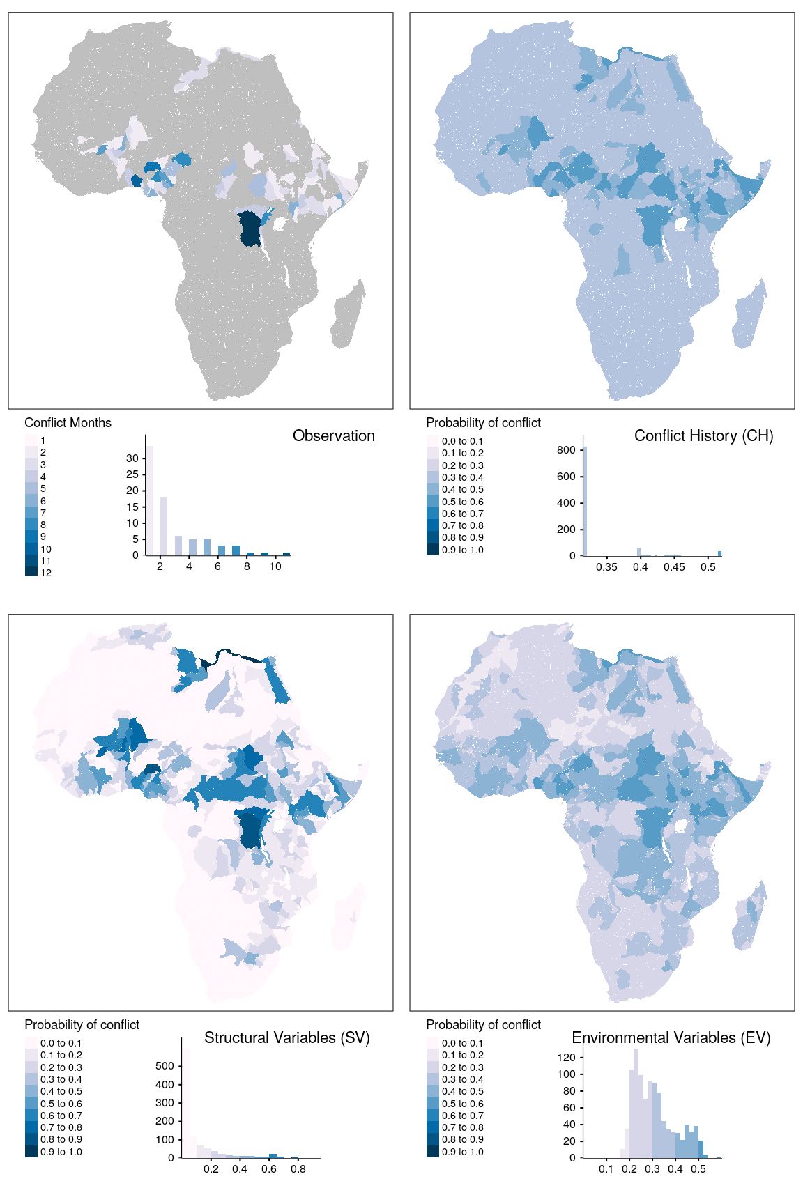
Figure 1.18: Spatial prediction of conflict class ns for bas districts.
map_data %>%
  filter(unit == "basins", var == "os") -> plt_data

breaks = seq(0,1,0.1)

plt_data %>%
  filter(type == "baseline") %>%
  dplyr::select(obsv) %>%
  mutate(obsv = ifelse(obsv > 0, obsv, NA)) -> obsv_data

obsv_data %>%
  tm_shape() +
  tm_polygons("obsv",
              palette = "PuBu",
              lwd=.01,
              border.col = "grey90",
              breaks = 0:12,
              style = "fixed",
              title = "Conflict Months",
              showNA = FALSE,
              legend.hist = TRUE,
              labels = as.character(1:12)) +
  tm_legend(stack = "horizontal") +
  tm_layout(title = "Observation",
            title.position = c("right", "top"),
            title.size = 0.7,
            legend.title.size = 0.7,
            legend.text.size = 0.45,
            legend.position = c("left", "bottom"),
            legend.outside.position = "bottom",
            legend.bg.color = "white",
            legend.bg.alpha = 0,
            legend.outside = TRUE,
            legend.hist.width = 1,
            legend.hist.height = .8,
            legend.hist.size = .5)   -> map_obsv

plt_data %>%
  filter(type == "baseline") %>%
  tm_shape() +
  tm_polygons("mean",
              palette = "PuBu",
              lwd=.01,
              border.col = "grey90",
              title = "Probability of conflict",
              breaks = breaks,
              style = "fixed",
              legend.hist = TRUE) +
  tm_legend(stack = "horizontal") +
  tm_layout(title = "Conflict History (CH)",
            title.position = c("right", "top"),
            title.size = 0.7,
            legend.title.size = 0.7,
            legend.text.size = 0.45,
            legend.position = c("left", "bottom"),
            legend.outside.position = "bottom",
            legend.bg.color = "white",
            legend.bg.alpha = 0,
            legend.outside = TRUE,
            legend.hist.width = 1,
            legend.hist.height = .8,
            legend.hist.size = .5)   -> map_bas

plt_data %>%
  filter(type == "structural") %>%
  tm_shape() +
  tm_polygons("mean",
              palette = "PuBu",
              lwd=.01,
              border.col = "grey90",
              title = "Probability of conflict",
              breaks = breaks,
              style = "fixed",
              legend.hist = TRUE)  +
  tm_legend(stack = "horizontal") +
  tm_layout(title = "Structural Variables (SV)",
            title.position = c("right", "top"),
            title.size = 0.7,
            legend.title.size = 0.7,
            legend.text.size = 0.45,
            legend.position = c("left", "bottom"),
            legend.outside.position = "bottom",
            legend.bg.color = "white",
            legend.bg.alpha = 0,
            legend.outside = TRUE,
            legend.hist.width = 1,
            legend.hist.height = .8,
            legend.hist.size = .5)  -> map_str

plt_data %>%
  filter(type == "environmental") %>%
  tm_shape() +
  tm_polygons("mean",
              palette = "PuBu",
              lwd=.01,
              border.col = "grey90",
              title = "Probability of conflict",
              breaks = breaks,
              style = "fixed",
              legend.hist = TRUE)  +
  tm_legend(stack = "horizontal") +
  tm_layout(title = "Environmental Variables (EV)",
            title.position = c("right", "top"),
            title.size = 0.7,
            legend.title.size = 0.7,
            legend.text.size = 0.45,
            legend.position = c("left", "bottom"),
            legend.outside.position = "bottom",
            legend.bg.color = "white",
            legend.bg.alpha = 0,
            legend.outside = TRUE,
            legend.hist.width = 1,
            legend.hist.height = .8,
            legend.hist.size = .5)  -> map_env

tmap_arrange(map_obsv, map_bas, map_str, map_env, ncol = 2)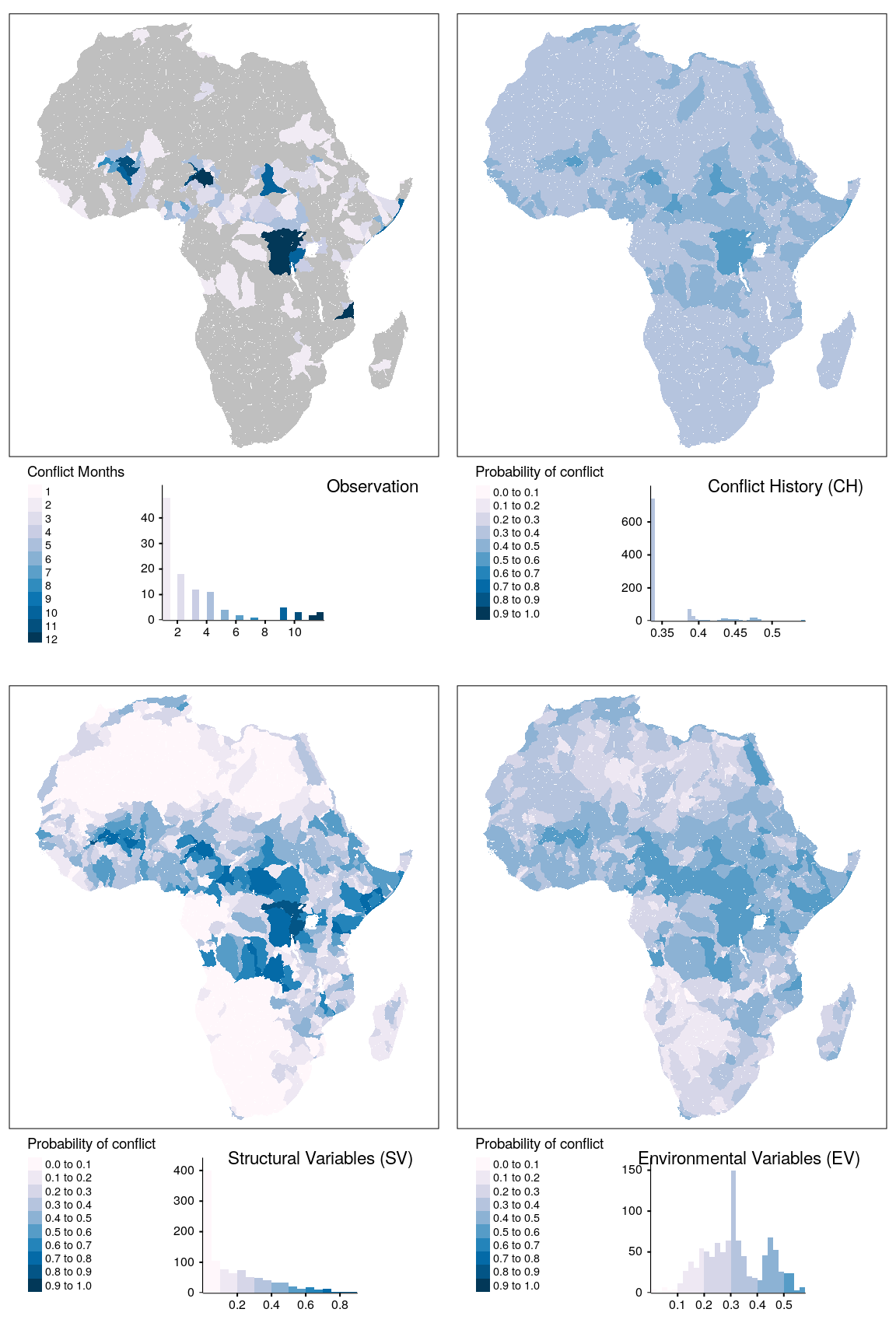
Figure 1.19: Spatial prediction of conflict class os for bas districts.
\end{tiny}
QQ-Plots and Residual Plots of Interaction Model
files <- list.files("../output/test-results/", pattern = "test-results", full.names = T)
acc_data <- lapply(files, function(x){
  out <- vars_detect(x)
  tmp = readRDS(x)
  tmp %<>%
    filter(name == "f2",
           month == 0)
  tmp$type = out$type
  tmp
})

acc_data = do.call(rbind, acc_data)
acc_data %<>%
  mutate(type = factor(type,
                       levels = c("regression", "baseline", "structural", "environmental"),
                       labels = c("LR", "CH", "SV", "EV")),
         var = factor(var,
                      levels = c("all", "sb", "ns", "os"),
                      labels = c("cb", "sb", "ns", "os")),
         unit = factor(unit,
                       levels = c("states", "basins"),
                       labels = c("adm", "bas")))

acc_data %>%
  # filter(type != "LR") %>%
  group_by(var) %>%
  nest() %>%
  mutate(model = map(data, ~lm(score ~ unit*type, data = .x)),
         model = map(model, ~augment(.x)),
         plots_resid= map(model,
                          ~ggplot(data = .x, aes(x=.fitted, y =.resid, shape = unit, color = type)) +
                            geom_point(alpha = .5) +
                            xlim(0.15,.7) +
                            labs(x="Fitted values",
                                 y = "Residuals",
                                 color = "Aggregation unit",
                                 shape = "Predictor set",
                                 subtitle = var) +
                            scale_color_brewer(palette = "Dark2") +
                            guides(colour = guide_legend(override.aes = list(alpha = 1)),
                                   shape = guide_legend(override.aes = list(alpha = 1))) +
                            theme_classic() +
                            theme(
                              plot.subtitle=element_markdown(face = "bold", hjust = .5),
                              plot.title = element_markdown(size = 10),
                              plot.caption = element_markdown(size = 10),
                              plot.tag = element_markdown(size = 10),
                              strip.background = element_blank(),
                              strip.text = element_markdown(size = 10),
                              strip.text.x = element_markdown(size = 10),
                              strip.text.y = element_markdown(size = 10),
                              legend.position = "bottom",
                              legend.key.size = unit(0.4, "cm"),
                              legend.text = element_markdown(size = 9),
                              legend.title = element_markdown(size=10),
                              axis.text = element_markdown(size = 7),
                              axis.title=element_markdown(size=10)
                            )),
         plots_qq = map(model,
                        ~ggplot(data = .x, aes(sample = score, shape = unit, color = type)) +
                          stat_qq(alpha = .55) +
                          ylim(0.05, 0.85) +
                          labs(x="Theoretical quantiles",
                               y = "Sample quantiles",
                               color = "Aggregation unit",
                               shape = "Predictor set",
                               subtitle = var) +
                          scale_color_brewer(palette = "Dark2") +
                          guides(colour = guide_legend(override.aes = list(alpha = 1)),
                                 shape = guide_legend(override.aes = list(alpha = 1))) +
                          theme_classic() +
                          theme(
                            plot.subtitle=element_markdown(face = "bold", hjust = .5),
                            plot.title = element_markdown(size = 10),
                            plot.caption = element_markdown(size = 10),
                            plot.tag = element_markdown(size = 10),
                            strip.background = element_blank(),
                            strip.text = element_markdown(size = 10),
                            strip.text.x = element_markdown(size = 10),
                            strip.text.y = element_markdown(size = 10),
                            legend.position = "bottom",
                            legend.key.size = unit(0.4, "cm"),
                            legend.text = element_markdown(size = 9),
                            legend.title = element_markdown(size=10),
                            axis.text = element_markdown(size = 7),
                            axis.title=element_markdown(size=10)
                          )
         )
  ) -> lm_plots
qqplots = lm_plots$plots_qq
if(knitr::is_latex_output()){
ggarrange(qqplots[[1]] +
theme(axis.title.x = element_blank(),
axis.text.x = element_blank(),
axis.ticks.x = element_blank(),
axis.line.x = element_blank()),
qqplots[[4]]+
theme(axis.title.x = element_blank(),
axis.text.x = element_blank(),
axis.ticks.x = element_blank(),
axis.line.x = element_blank(),
axis.title.y = element_blank(),
axis.text.y = element_blank(),
axis.ticks.y = element_blank(),
axis.line.y = element_blank()),
qqplots[[2]],
qqplots[[3]] +
theme(axis.title.y = element_blank(),
axis.text.y = element_blank(),
axis.ticks.y = element_blank(),
axis.line.y = element_blank()),
ncol = 2, nrow = 2, common.legend = TRUE, legend="bottom")
} else {
for (i in 1:length(qqplots)){
var = as.character(qqplots[[i]]$labels$subtitle)
require(plotly)
ggplotly(qqplots[[i]] + ggtitle(var) + theme(plot.title = element_markdown(face = "bold"))) %>%
layout(legend = list(orientation = "h",
xanchor = "center",
x = 0.5, y = -.2)) -> plt_out
print(plt_out)
}
}residplots = lm_plots$plots_resid
if(knitr::is_latex_output()){
ggarrange(residplots[[1]] +
theme(axis.title.x = element_blank(),
axis.text.x = element_blank(),
axis.ticks.x = element_blank(),
axis.line.x = element_blank()),
residplots[[4]]+
theme(axis.title.x = element_blank(),
axis.text.x = element_blank(),
axis.ticks.x = element_blank(),
axis.line.x = element_blank(),
axis.title.y = element_blank(),
axis.text.y = element_blank(),
axis.ticks.y = element_blank(),
axis.line.y = element_blank()),
residplots[[2]],
residplots[[3]] +
theme(axis.title.y = element_blank(),
axis.text.y = element_blank(),
axis.ticks.y = element_blank(),
axis.line.y = element_blank()),
ncol = 2, nrow = 2, common.legend = TRUE, legend="bottom")
} else {
for (i in 1:length(residplots)){
var = as.character(residplots[[i]]$labels$subtitle)
require(plotly)
ggplotly(residplots[[i]] + ggtitle(var) + theme(plot.title = element_markdown(face = "bold"))) %>%
layout(legend = list(orientation = "h",
xanchor = "center",
x = 0.5, y = -.2)) -> plt_out
print(plt_out)
}
}Descriptive Statistics of Interaction Variables with Agricultural Mask
predictors = readRDS("../data/vector/predictor_cube.rds")
vars = c("AGRET", "AGRGPP", "AGRLST", "AGRPREC", "AGRANOM", "AGRSPI1", "AGRSPI3", "AGRSPI6", "AGRSPI12", "AGRSPEI1", "AGRSPEI3", "AGRSPEI6", "AGRSPEI12")
predictors %>%
  filter(var %in% vars) %>%
  as_tibble() %>%
  mutate(var = factor(var,
                      labels = vars,
                      levels = vars)) %>%
  dplyr::select(id, unit, var, value) %>%
  filter(!(unit == "states" & id > 847)) %>%
  group_by(unit, var) %>%
  summarise("Min." = round(min(value, na.rm = T),3),
            "1st Qu." = round(quantile(value, 0.25, na.rm = T),3),
            "Median" = round(median(value, na.rm = T),3),
            "Mean" = round(mean(value, na.rm = T),3),
            "3rd Qu." = round(quantile(value, 0.75, na.rm = T),3),
            "Max." = round(max(value, na.rm = T),3),
            "NA's" = round(sum(is.na(value)),3)) %>%
  ungroup() %>%
  mutate(unit = if_else(unit == "basins","*bas*", "*adm*")) %>%
  mutate(unit = factor(unit, levels = c("*adm*", "*bas*"),
                       labels = c("*adm*", "*bas*"))) %>%
  arrange(var, unit) %>%
  dplyr::select(-var) %>%
  rename("Spatial Unit" = unit) %>%
  thesis_kable(escape = FALSE,
               caption = "Descriptive statistics of agricultural interaction variables. (Unit of measurment: AGRET - kg/m²; AGRGPP - kg C/m²; AGRLST - K; AGRPREC - mm AGRANOM - mm; others - dimensionless)",
               caption.short = "Descriptive statistics of agricultural interaction variables.",
               linesep = c("", "\\addlinespace"),
               longtable = T) %>%
  kable_styling(latex_options = c("HOLD_position", "repeat_header")) %>%
  group_rows("AGRET", 1, 2) %>%
  group_rows("AGRGPP", 3, 4) %>%
  group_rows("AGRLST", 5, 6) %>%
  group_rows("AGRPREC", 7, 8) %>%
  group_rows("AGRANOM", 9, 10) %>%
  group_rows("AGRSPI1", 11, 12) %>%
  group_rows("AGRSPI3", 13, 14) %>%
  group_rows("AGRSPI6", 15, 16) %>%
  group_rows("AGRSPI12", 17, 18) %>%
  group_rows("AGRSPEI1", 19, 20) %>%
  group_rows("AGRSPEI3", 21, 22) %>%
  group_rows("AGRSPEI6", 23, 24) %>%
group_rows("AGRSPEI12", 25, 26)| Spatial Unit | Min. | 1st Qu. | Median | Mean | 3rd Qu. | Max. | NA’s |
|---|---|---|---|---|---|---|---|
| AGRET | |||||||
| adm | 0.000 | 0.253 | 9.996 | 118.725 | 138.828 | 1273.573 | 643 |
| bas | 0.000 | 0.000 | 0.647 | 28.715 | 12.693 | 973.495 | 39358 |
| AGRGPP | |||||||
| adm | 0.000 | 0.491 | 20.158 | 232.349 | 272.386 | 6251.350 | 478 |
| bas | 0.000 | 0.000 | 1.337 | 55.510 | 27.987 | 2465.299 | 38957 |
| AGRLST | |||||||
| adm | 0.000 | 0.137 | 8.428 | 60.278 | 104.179 | 312.276 | 0 |
| bas | 0.000 | 0.000 | 0.066 | 18.272 | 7.486 | 279.603 | 0 |
| AGRPREC | |||||||
| adm | 0.000 | 0.003 | 0.526 | 17.237 | 13.174 | 429.346 | 0 |
| bas | 0.000 | 0.000 | 0.001 | 4.473 | 0.500 | 304.854 | 0 |
| AGRANOM | |||||||
| adm | -154.115 | -0.148 | 0.000 | 0.535 | 0.050 | 265.607 | 0 |
| bas | -138.119 | -0.001 | 0.000 | 0.082 | 0.000 | 125.800 | 0 |
| AGRSPI1 | |||||||
| adm | -3.554 | -0.006 | 0.000 | 0.011 | 0.004 | 5.854 | 1100 |
| bas | -3.471 | 0.000 | 0.000 | 0.003 | 0.000 | 4.494 | 2571 |
| AGRSPI3 | |||||||
| adm | -4.829 | -0.004 | 0.000 | 0.012 | 0.007 | 5.773 | 2654 |
| bas | -2.411 | 0.000 | 0.000 | 0.003 | 0.000 | 3.517 | 3331 |
| AGRSPI6 | |||||||
| adm | -3.935 | -0.003 | 0.000 | 0.012 | 0.008 | 4.157 | 5180 |
| bas | -2.596 | 0.000 | 0.000 | 0.003 | 0.000 | 3.035 | 6005 |
| AGRSPI12 | |||||||
| adm | -4.750 | -0.003 | 0.000 | 0.012 | 0.008 | 3.555 | 10233 |
| bas | -2.481 | 0.000 | 0.000 | 0.003 | 0.000 | 2.726 | 12059 |
| AGRSPEI1 | |||||||
| adm | -4.126 | -0.005 | 0.000 | 0.007 | 0.006 | 3.306 | 973 |
| bas | -2.446 | 0.000 | 0.000 | 0.002 | 0.000 | 2.427 | 2230 |
| AGRSPEI3 | |||||||
| adm | -2.740 | -0.005 | 0.000 | 0.008 | 0.006 | 5.006 | 2651 |
| bas | -1.819 | 0.000 | 0.000 | 0.002 | 0.000 | 2.636 | 3310 |
| AGRSPEI6 | |||||||
| adm | -2.423 | -0.004 | 0.000 | 0.008 | 0.007 | 4.259 | 5183 |
| bas | -1.856 | 0.000 | 0.000 | 0.002 | 0.000 | 2.730 | 6005 |
| AGRSPEI12 | |||||||
| adm | -3.134 | -0.004 | 0.000 | 0.007 | 0.007 | 3.558 | 10246 |
| bas | -2.689 | 0.000 | 0.000 | 0.002 | 0.000 | 2.668 | 12059 |
Table of Global Performance Metrics
#files <- list.files("../output/acc/", pattern = ".rds", full.names = T)
files <- list.files("../output/test-results/", pattern = "test-results", full.names = T)
# files <- files[-grep("test-results-regression-basins", files)]
acc_data <- lapply(files, function(x){
  out <- vars_detect(x)
  tmp = readRDS(x)
  tmp %>%
    filter(month == 0) %>%
    group_by(name) %>%
    summarise(target = mean(score, na.rm = T),
              sd = sd(score, na.rm = T),
              type = out$type,
              unit = out$unit,
              var = out$var) %>%
    ungroup()
})
acc_data = do.call(rbind, acc_data)

acc_data %<>%
  mutate(var = factor(var, labels = c("**cb**", "**sb**", "**ns**", "**os**"),
                      levels = c("all", "sb", "ns", "os")),
         type = factor(type, labels = c("LR", "CH", "SV", "EV"),
                       levels = c("regression", "baseline", "structural", "environmental")),
         unit = if_else(unit == "basins", "bas", "adm"),
         unit = factor(unit, levels = c("adm", "bas"), labels = c("\\emph{adm}", "\\emph{bas}")))

acc_data %>%
  filter(name %in% c("f2", "auc", "aucpr", "sensitivity", "specificity", "precision")) %>%
  mutate(
    sd = paste0("(", as.character(round(sd,3)), ")"),
    score = paste0(round(target,3), " +/- ", sd)) %>%
  dplyr::select(type, unit, var, name, score, target) %>%
  group_by(name, var) %>%
  mutate(score = if_else(target == max(target), paste0("**", score, "**"), score )) %>%
  dplyr::select(-target) %>%
  ungroup() %>%
  pivot_wider(names_from = name, values_from = c(score),
              id_cols = c(type, unit, var)) %>%
  arrange(type, unit, var) %>%
  rename("F2" = f2, "AUC" = auc, "AUPR" = aucpr, "Precision" = precision, "Sensitivity" = sensitivity, "Specificity" = specificity) %>%
  rename(Theme = type, Unit = "unit", Variable = var) %>%
  relocate(Theme, Unit, Variable, F2, AUC, AUPR, Precision, Sensitivity, Specificity) %>%
  ungroup %>%
  thesis_kable(escape = F,
               align = "ccccccccc",
               longtable = T,
               linesep = c("", "", "","\\addlinespace"),
               caption.short = "Global performance metrics for all model configurations.",
               caption = "Global performance metrics for all models configurations. Bold number indicate the best performance of the respective performance metric per conflict class. Standard deviation is given in brackets.") %>%
kable_styling(latex_options = c("HOLD_position", "repeat_header"))| Theme | Unit | Variable | F2 | AUC | AUPR | Precision | Sensitivity | Specificity |
|---|---|---|---|---|---|---|---|---|
| LR | cb | 0.325 +/- (0.001) | 0.671 +/- (0.001) | 0.128 +/- (0.001) | 0.11 +/- (0.002) | 0.668 +/- (0.007) | 0.598 +/- (0.007) | |
| LR | sb | 0.242 +/- (0.003) | 0.703 +/- (0.003) | 0.084 +/- (0.002) | 0.08 +/- (0.002) | 0.541 +/- (0.02) | 0.751 +/- (0.014) | |
| LR | ns | 0.183 +/- (0.002) | 0.739 +/- (0.002) | 0.049 +/- (0.001) | 0.055 +/- (0.002) | 0.468 +/- (0.032) | 0.842 +/- (0.019) | |
| LR | os | 0.226 +/- (0.002) | 0.681 +/- (0.002) | 0.072 +/- (0.001) | 0.075 +/- (0.001) | 0.494 +/- (0.02) | 0.777 +/- (0.014) | |
| LR | cb | 0.389 +/- (0.001) | 0.758 +/- (0.001) | 0.168 +/- (0.001) | 0.141 +/- (0.003) | 0.708 +/- (0.016) | 0.687 +/- (0.014) | |
| LR | sb | 0.302 +/- (0.002) | 0.775 +/- (0.003) | 0.121 +/- (0.002) | 0.105 +/- (0.003) | 0.592 +/- (0.019) | 0.8 +/- (0.012) | |
| LR | ns | 0.216 +/- (0.002) | 0.779 +/- (0.003) | 0.069 +/- (0.002) | 0.073 +/- (0.003) | 0.477 +/- (0.022) | 0.867 +/- (0.013) | |
| LR | os | 0.287 +/- (0.003) | 0.774 +/- (0.003) | 0.105 +/- (0.002) | 0.1 +/- (0.002) | 0.549 +/- (0.012) | 0.83 +/- (0.007) | |
| CH | cb | 0.59 +/- (0.027) | 0.918 +/- (0.002) | 0.6 +/- (0.008) | 0.283 +/- (0.046) | 0.824 +/- (0.041) | 0.845 +/- (0.045) | |
| CH | sb | 0.604 +/- (0.045) | 0.943 +/- (0.006) | 0.634 +/- (0.019) | 0.297 +/- (0.069) | 0.832 +/- (0.022) | 0.923 +/- (0.023) | |
| CH | ns | 0.467 +/- (0.044) | 0.943 +/- (0.003) | 0.359 +/- (0.024) | 0.178 +/- (0.043) | 0.828 +/- (0.073) | 0.922 +/- (0.029) | |
| CH | os | 0.486 +/- (0.022) | 0.909 +/- (0.003) | 0.472 +/- (0.01) | 0.207 +/- (0.027) | 0.743 +/- (0.031) | 0.902 +/- (0.021) | |
| CH | cb | 0.664 +/- (0.014) | 0.942 +/- (0.013) | 0.573 +/- (0.107) | 0.395 +/- (0.084) | 0.822 +/- (0.073) | 0.916 +/- (0.034) | |
| CH | sb | 0.607 +/- (0.087) | 0.954 +/- (0.003) | 0.518 +/- (0.048) | 0.552 +/- (0.08) | 0.635 +/- (0.125) | 0.982 +/- (0.01) | |
| CH | ns | 0.375 +/- (0.107) | 0.92 +/- (0.047) | 0.266 +/- (0.04) | 0.335 +/- (0.054) | 0.404 +/- (0.151) | 0.986 +/- (0.007) | |
| CH | os | 0.5 +/- (0.039) | 0.925 +/- (0.006) | 0.42 +/- (0.05) | 0.295 +/- (0.114) | 0.683 +/- (0.151) | 0.937 +/- (0.048) | |
| SV | cb | 0.616 +/- (0.009) | 0.92 +/- (0.007) | 0.599 +/- (0.011) | 0.402 +/- (0.036) | 0.715 +/- (0.037) | 0.923 +/- (0.015) | |
| SV | sb | 0.633 +/- (0.022) | 0.947 +/- (0.006) | 0.613 +/- (0.022) | 0.455 +/- (0.044) | 0.706 +/- (0.044) | 0.968 +/- (0.008) | |
| SV | ns | 0.398 +/- (0.085) | 0.933 +/- (0.006) | 0.322 +/- (0.021) | 0.345 +/- (0.09) | 0.45 +/- (0.155) | 0.98 +/- (0.014) | |
| SV | os | 0.493 +/- (0.026) | 0.906 +/- (0.01) | 0.426 +/- (0.016) | 0.275 +/- (0.048) | 0.638 +/- (0.1) | 0.94 +/- (0.023) | |
| SV | cb | 0.649 +/- (0.014) | 0.948 +/- (0.003) | 0.625 +/- (0.011) | 0.32 +/- (0.021) | 0.876 +/- (0.016) | 0.886 +/- (0.013) | |
| SV | sb | 0.671 +/- (0.026) | 0.963 +/- (0.004) | 0.617 +/- (0.028) | 0.356 +/- (0.036) | 0.865 +/- (0.025) | 0.948 +/- (0.01) | |
| SV | ns | 0.452 +/- (0.02) | 0.94 +/- (0.005) | 0.275 +/- (0.026) | 0.191 +/- (0.022) | 0.696 +/- (0.046) | 0.95 +/- (0.009) | |
| SV | os | 0.518 +/- (0.033) | 0.941 +/- (0.006) | 0.48 +/- (0.026) | 0.241 +/- (0.041) | 0.747 +/- (0.074) | 0.928 +/- (0.031) | |
| EV | cb | 0.618 +/- (0.009) | 0.924 +/- (0.003) | 0.609 +/- (0.007) | 0.401 +/- (0.044) | 0.72 +/- (0.048) | 0.922 +/- (0.02) | |
| EV | sb | 0.647 +/- (0.026) | 0.947 +/- (0.005) | 0.65 +/- (0.012) | 0.394 +/- (0.072) | 0.783 +/- (0.039) | 0.953 +/- (0.015) | |
| EV | ns | 0.438 +/- (0.038) | 0.936 +/- (0.007) | 0.298 +/- (0.058) | 0.275 +/- (0.091) | 0.565 +/- (0.144) | 0.967 +/- (0.018) | |
| EV | os | 0.508 +/- (0.012) | 0.903 +/- (0.008) | 0.431 +/- (0.02) | 0.237 +/- (0.027) | 0.719 +/- (0.042) | 0.921 +/- (0.016) | |
| EV | cb | 0.689 +/- (0.006) | 0.951 +/- (0.003) | 0.639 +/- (0.021) | 0.418 +/- (0.026) | 0.824 +/- (0.017) | 0.93 +/- (0.009) | |
| EV | sb | 0.67 +/- (0.021) | 0.963 +/- (0.003) | 0.616 +/- (0.021) | 0.42 +/- (0.036) | 0.791 +/- (0.038) | 0.964 +/- (0.007) | |
| EV | ns | 0.487 +/- (0.016) | 0.947 +/- (0.004) | 0.305 +/- (0.025) | 0.249 +/- (0.028) | 0.647 +/- (0.051) | 0.967 +/- (0.007) | |
| EV | os | 0.553 +/- (0.014) | 0.944 +/- (0.003) | 0.5 +/- (0.011) | 0.308 +/- (0.035) | 0.697 +/- (0.04) | 0.954 +/- (0.01) |
sessionInfo()R version 3.6.3 (2020-02-29)
Platform: x86_64-pc-linux-gnu (64-bit)
Running under: Debian GNU/Linux 10 (buster)
Matrix products: default
BLAS/LAPACK: /usr/lib/x86_64-linux-gnu/libopenblasp-r0.3.5.so
locale:
[1] LC_CTYPE=en_US.UTF-8 LC_NUMERIC=C
[3] LC_TIME=en_US.UTF-8 LC_COLLATE=en_US.UTF-8
[5] LC_MONETARY=en_US.UTF-8 LC_MESSAGES=C
[7] LC_PAPER=en_US.UTF-8 LC_NAME=C
[9] LC_ADDRESS=C LC_TELEPHONE=C
[11] LC_MEASUREMENT=en_US.UTF-8 LC_IDENTIFICATION=C
attached base packages:
[1] stats graphics grDevices utils datasets methods base
other attached packages:
[1] plotly_4.9.2.1 lubridate_1.7.9.2 rgdal_1.5-18 countrycode_1.2.0
[5] welchADF_0.3.2 rstatix_0.6.0 ggpubr_0.4.0 scales_1.1.1
[9] RColorBrewer_1.1-2 latex2exp_0.4.0 cubelyr_1.0.0 gridExtra_2.3
[13] ggtext_0.1.1 magrittr_2.0.1 tmap_3.2 sf_0.9-7
[17] raster_3.4-5 sp_1.4-4 forcats_0.5.0 stringr_1.4.0
[21] purrr_0.3.4 readr_1.4.0 tidyr_1.1.2 tibble_3.0.6
[25] tidyverse_1.3.0 huwiwidown_0.0.1 kableExtra_1.3.1 knitr_1.31
[29] rmarkdown_2.7.3 bookdown_0.21 ggplot2_3.3.3 dplyr_1.0.2
[33] devtools_2.3.2 usethis_2.0.0
loaded via a namespace (and not attached):
[1] readxl_1.3.1 backports_1.2.0 workflowr_1.6.2
[4] lwgeom_0.2-5 lazyeval_0.2.2 splines_3.6.3
[7] crosstalk_1.1.0.1 leaflet_2.0.3 digest_0.6.27
[10] htmltools_0.5.1.1 memoise_1.1.0 openxlsx_4.2.3
[13] remotes_2.2.0 modelr_0.1.8 prettyunits_1.1.1
[16] colorspace_2.0-0 rvest_0.3.6 haven_2.3.1
[19] xfun_0.21 leafem_0.1.3 callr_3.5.1
[22] crayon_1.4.0 jsonlite_1.7.2 lme4_1.1-26
[25] glue_1.4.2 stars_0.4-3 gtable_0.3.0
[28] webshot_0.5.2 car_3.0-10 pkgbuild_1.2.0
[31] abind_1.4-5 DBI_1.1.0 Rcpp_1.0.5
[34] viridisLite_0.3.0 gridtext_0.1.4 units_0.6-7
[37] foreign_0.8-71 htmlwidgets_1.5.3 httr_1.4.2
[40] ellipsis_0.3.1 farver_2.0.3 pkgconfig_2.0.3
[43] XML_3.99-0.3 dbplyr_2.0.0 labeling_0.4.2
[46] tidyselect_1.1.0 rlang_0.4.10 later_1.1.0.1
[49] tmaptools_3.1 munsell_0.5.0 cellranger_1.1.0
[52] tools_3.6.3 cli_2.3.0 generics_0.1.0
[55] broom_0.7.2 evaluate_0.14 yaml_2.2.1
[58] processx_3.4.5 leafsync_0.1.0 fs_1.5.0
[61] zip_2.1.1 nlme_3.1-150 xml2_1.3.2
[64] compiler_3.6.3 rstudioapi_0.13 curl_4.3
[67] png_0.1-7 e1071_1.7-4 testthat_3.0.1
[70] ggsignif_0.6.0 reprex_0.3.0 statmod_1.4.35
[73] stringi_1.5.3 highr_0.8 ps_1.5.0
[76] desc_1.2.0 lattice_0.20-41 Matrix_1.2-18
[79] markdown_1.1 nloptr_1.2.2.2 classInt_0.4-3
[82] vctrs_0.3.6 pillar_1.4.7 lifecycle_0.2.0
[85] data.table_1.13.2 httpuv_1.5.5 R6_2.5.0
[88] promises_1.1.1 KernSmooth_2.23-18 rio_0.5.16
[91] sessioninfo_1.1.1 codetools_0.2-16 dichromat_2.0-0
[94] boot_1.3-25 MASS_7.3-53 assertthat_0.2.1
[97] pkgload_1.1.0 rprojroot_2.0.2 withr_2.4.1
[100] mgcv_1.8-33 parallel_3.6.3 hms_1.0.0
[103] grid_3.6.3 minqa_1.2.4 class_7.3-17
[106] carData_3.0-4 git2r_0.27.1 base64enc_0.1-3