Last updated: 2021-03-24
Checks: 5 1
Knit directory:
thesis/analysis/
This reproducible R Markdown analysis was created with workflowr (version 1.6.2). The Checks tab describes the reproducibility checks that were applied when the results were created. The Past versions tab lists the development history.
Great job! The global environment was empty. Objects defined in the global environment can affect the analysis in your R Markdown file in unknown ways. For reproduciblity it’s best to always run the code in an empty environment.
The command set.seed(20210321) was run prior to running the code in the R Markdown file.
Setting a seed ensures that any results that rely on randomness,
e.g. subsampling or permutations, are reproducible.
Great job! Recording the operating system, R version, and package versions is critical for reproducibility.
Nice! There were no cached chunks for this analysis, so you can be confident that you successfully produced the results during this run.
Great job! Using relative paths to the files within your workflowr project makes it easier to run your code on other machines.
Tracking code development and connecting the code version to the results is
critical for reproducibility. To start using Git, open the Terminal and type
git init in your project directory.
This project is not being versioned with Git. To obtain the full
reproducibility benefits of using workflowr, please see
?wflow_start.
1 Results and Discussion
1.1 Hyperparameter Tuning
The results of the BO process are reported in Table 1.1. For each of the predictor sets, an optimization was conducted for both the adm and bas units. Except for the SV-bas model, a double-layered CNN was found to deliver the best results. Concerning the activation function \(a_{cnn}\), the picture is less clear, but softmax was selected in \(\frac{8}{24}\) of the cases followed by the hard_sigmoid activation function (\(\frac{7}{24}\)). The kernel numbers \(k_{cnn}\) are selected only twice above a value of 120, approximating the maximum possible value of 128. The size of the network generally seems sufficient to capture the data structure. The selected kernel widths \(\beta_{cnn}\) for the CH-bas model are at the maximum of 24 months for both the 50 and 100 km branch, suggesting that for this variable configuration, there could be a performance improvement with bigger kernel widths. For the remaining configurations, the kernel widths are mainly between five to 22 months. For parameter \(pool_1\), in about half the cases maximum pooling is selected with \(pool\_size\) between 3 and 24 and only in \(\frac{6}{24}\) cases the pool size is below 12. Generally, information beyond a period of 12 months seems to represent the signal for conflicts better. As pooling operation \(pool_2\), maximum pooling is selected in \(\frac{17}{24}\) cases, indicating that maximizing the values through the time series is beneficial for the conflict prediction task. It is of interest that average pooling was only chosen for 100 and 200 km inputs. The signal from these inputs seems to be better represented by an average layer.
For most variable configurations, the selection of two LSTM-layers yielded the best results, except for the CH-bas and EV-adm configurations. Similar to the CNN part of the model, the results suggest that the sizes of \(n_{1:3}\) generally seem to be sufficient for the data complexity. Only in \(\frac{7}{72}\) cases more than 120 neurons are selected for a LSTM layer. Instead, the number of neurons is frequently below 100, indicating that smaller network sizes are able to learn a pattern from the data. There is no clear pattern concerning the number of neurons across variable configurations or between layers. Also, dropout rates \(d_{1:3}\) vary substantially, with the lowest rate of 1 % to the highest of 50 % dropout. As the activation function \(a_{dense}\) for the fully connected model, softplus and relu both are selected twice. The number of neurons \(n_{dense}\) is between 21 and 97 neurons. The maximum of 128 is not approximated by any of the model configurations.
files <- list.files("../output/bayes/", ".rds$", full.names = T)

results <- lapply(files, function(x){
  data <- readRDS(x)
  if(str_detect(x, "baseline")) type <- "baseline"
  if(str_detect(x, "structural")) type <- "structural"
  if(str_detect(x, "environmental")) type <- "environmental"
  if(str_detect(x, "basins")) unit <- "bas"
  if(str_detect(x, "states")) unit <- "adm"
  data[str_detect(data, "average")] = "avg."
  paras <- tibble(
    '$double\\_cnn$' = NA,
    '$a_{cnn}$' = NA,
    '$k_{cnn}$' = NA,
    '$\\beta_{cnn}$' = NA,
    "$pool_1$" = NA,
    "$pool\\_size$" = NA,
    '$pool_2$' = NA,
    '$lstm\\_layers$' = NA,
    '$n_1$' = NA,
    '$d_1$' = NA,
    '$n_2$' = NA,
    '$d_2$' = NA,
    '$n_3$' = NA,
    '$d_3$' = NA,
    '$a_{dense}$' = NA,
    '$n_{dense}$' = NA,
    '$a_{out}$' = NA,
    '$\\pi$' = NA,
    '$\\alpha$' = NA,
    '$\\gamma$' = NA,
    '$opti$' = NA,
    '$lr$' = NA)

  double_cnns = data[rep(grep("double_cnn", names(data)),4)]
  paras[,1] = paste(if_else(double_cnns == TRUE, "$Yes$", "$No$"), collapse = "/")
  paras[,2] = paste(data[grep("cnn_activation", names(data))], collapse = "/")
  paras[,3] = paste(data[grep("cnn_filters", names(data))], collapse = "/")
  paras[,4] = paste(data[grep("cnn_kernel", names(data))], collapse = "/")
  paras[,5] = paste(data[grep("cnn_pooling", names(data))], collapse = "/")
  paras[,6] = paste(data[grep("pool_size", names(data))], collapse = "/")
  paras[,7] = paste(data[grep("global_pooling", names(data))], collapse = "/")
  paras[,8] = paste(rep(data[grep("lstm_layers", names(data))], 4), collapse = "/")

  paras[,9] = paste(data[grep("lstm_neurons_1", names(data))], collapse = "/")
  paras[,10] = paste(round(unlist(data[grep("lstm_dropout_1", names(data))]), 2), collapse = "/")

  inputs = c("inputUnit", "inputB50", "inputB100", "inputB200")

  neurons_2 = unlist(lapply(inputs, function(i){
    tmp = unlist(data[paste0(i,"_lstm_neurons_2")])
    if(is.null(tmp)) return("-")
    tmp
  }))
  neurons_2 = paste(neurons_2, collapse = "/")

  dropout_2 = unlist(lapply(inputs, function(i){
    tmp = unlist(data[paste0(i,"_lstm_dropout_2")])
    if(is.null(tmp)) return("-")
    round(tmp,2)
  }))
  dropout_2 = paste(dropout_2, collapse = "/")
  paras[,11] = neurons_2
  paras[,12] = dropout_2

  neurons_3 = unlist(lapply(inputs, function(i){
    tmp = unlist(data[paste0(i,"_lstm_neurons_3")])
    if(is.null(tmp)) return("-")
    tmp
  }))
  neurons_3 = paste(neurons_3, collapse = "/")

  dropout_3 = unlist(lapply(inputs, function(i){
    tmp = unlist(data[paste0(i,"_lstm_dropout_3")])
    if(is.null(tmp)) return("-")
    round(tmp,3)
  }))
  dropout_3 = paste(dropout_3, collapse = "/")
  paras[,13] = neurons_3
  paras[,14] = dropout_3

  paras[,15] = data$dense_activation
  paras[,16] = data$dense_units
  paras[,17] = data$out_activation
  paras[,18] = round(data$pi, 4)
  paras[,19] = round(data$alpha, 4)
  paras[,20] = round(data$gamma, 4)
  paras[,21] = data$optimizer
  paras[,22] = round(data$lr, 4)

  paras$unit = unit
  paras$type = type
  paras
})

results = do.call(rbind, results)
results$unit = factor(results$unit,
                      levels = c("adm", "bas"),
                      labels = c("$_adm_$", "$_bas_$"))
results$type = factor(results$type,
                      levels = c("baseline", "structural", "environmental"),
                      labels = c("Conflict History", "Structural Variables", "Environmental Variables"))


results["$a_{cnn}$"] = paste("$",sub("(/.*?)/(.*)", "\\1\\\\\\\\\\2", unlist(results["$a_{cnn}$"])), "$", sep = "")
results["$a_{cnn}$"] = str_replace_all(unlist(results["$a_{cnn}$"]), "_", "\\\\_")
results["$pool_1$"] = paste("$",unlist(results["$pool_1$"]), "$", sep = "")
results["$pool_2$"] = paste("$",unlist(results["$pool_2$"]), "$", sep = "")
results["$a_{dense}$"] = paste("$",str_replace(unlist(results["$a_{dense}$"]), "_", "\\\\_"), "$", sep = "")
results["$a_{out}$"] =  paste("$",str_replace(unlist(results["$a_{out}$"]), "_", "\\\\_"), "$", sep = "")
results["$opti$"] =  paste("$",str_replace(unlist(results["$opti$"]), "_", "\\\\_"), "$", sep = "")

results %>%
  arrange(type, unit) %>%
  mutate_all(as.character) %>%
  #mutate('$double\\_cnn$' = str_replace( .[,2],pattern = "TRUE", "$Yes$")) %>%
  pivot_longer(cols = 1:22, names_to = "Parameter") %>%
  pivot_wider(id_cols = c(Parameter), names_from = c(type, unit)) %>%
  # slice(1:17) %>%
  thesis_kable(
    align = c("lcccccc"),
    col.names = NULL,
    linesep = c(""),
    escape = F,
    caption = c("Results of the Bayesian hyperparameter optimization.")
  ) %>%
  kable_styling(latex_options = "HOLD_position", font_size = 8)   %>%
  add_header_above(c(" ", "adm" = 1, "bas" = 1, "adm" = 1, "bas"= 1, "adm" = 1, "bas" = 1), italic = T) %>%
  add_header_above(c(" ", "Conflict History (CH)" = 2, "Structural Variables (SV)" = 2, "Environmental Variables (EV)" = 2), bold = T) %>%
  footnote(general = "Multiple values indicate the results for the input branch of buffer size 0/50/100/200 km, respecitvley.",
           threeparttable = T,
           escape = FALSE,
           general_title = "General:",
footnote_as_chunk = T)| \(double\_cnn\) | \(Yes\)/\(Yes\)/\(Yes\)/\(Yes\) | \(Yes\)/\(Yes\)/\(Yes\)/\(Yes\) | \(Yes\)/\(Yes\)/\(Yes\)/\(Yes\) | \(No\)/\(No\)/\(No\)/\(No\) | \(Yes\)/\(Yes\)/\(Yes\)/\(Yes\) | \(Yes\)/\(Yes\)/\(Yes\)/\(Yes\) |
| \(a_{cnn}\) | \(softsign/hard\_sigmoid\\softsign/softmax\) | \(softsign/hard\_sigmoid\\sigmoid/softsign\) | \(softmax/softmax\\hard\_sigmoid/softmax\) | \(sigmoid/softplus\\softplus/softmax\) | \(hard\_sigmoid/softmax\\hard\_sigmoid/hard\_sigmoid\) | \(softmax/softmax\\hard\_sigmoid/softmax\) |
| \(k_{cnn}\) | 106/125/45/78 | 86/99/39/128 | 95/70/63/42 | 41/102/67/43 | 19/41/94/99 | 92/76/66/42 |
| \(\beta_{cnn}\) | 5/10/22/8 | 19/24/24/6 | 10/9/9/16 | 22/12/14/5 | 12/6/13/14 | 8/10/10/17 |
| \(pool_1\) | \(max/max/avg./max\) | \(avg./max/max/max\) | \(max/avg./avg./max\) | \(avg./max/avg./avg.\) | \(max/avg./max/avg.\) | \(max/avg./avg./max\) |
| \(pool\_size\) | 15/23/3/14 | 24/19/10/21 | 12/18/17/18 | 16/6/10/9 | 12/16/9/22 | 12/18/17/16 |
| \(pool_2\) | \(max/max/max/avg.\) | \(max/max/avg./avg.\) | \(max/max/max/avg.\) | \(max/max/avg./max\) | \(max/max/max/avg.\) | \(max/max/max/avg.\) |
| \(lstm\_layers\) | 2/2/2/2 | 3/3/3/3 | 2/2/2/2 | 2/2/2/2 | 3/3/3/3 | 2/2/2/2 |
| \(n_1\) | 114/83/114/106 | 97/12/12/78 | 109/128/43/23 | 23/59/38/92 | 88/28/85/122 | 107/127/38/18 |
| \(d_1\) | 0.22/0.08/0.14/0.49 | 0.23/0.2/0.38/0.25 | 0.02/0.09/0.07/0.06 | 0.22/0.14/0.02/0.2 | 0.2/0.1/0.09/0.31 | 0.02/0.07/0.05/0.06 |
| \(n_2\) | 79/53/62/123 | 128/34/84/65 | 83/82/128/21 | 37/114/83/56 | 111/19/13/104 | 76/80/128/21 |
| \(d_2\) | 0.05/0.28/0.37/0.08 | 0.5/0.24/0.05/0.16 | 0.34/0.03/0/0.29 | 0.26/0.12/0.46/0.47 | 0.23/0.04/0.09/0.49 | 0.34/0.02/0.01/0.31 |
| \(n_3\) | -/-/-/- | 85/92/96/57 | -/-/-/- | -/-/-/- | 54/109/106/13 | -/-/-/- |
| \(d_3\) | -/-/-/- | 0.437/0.231/0.255/0.172 | -/-/-/- | -/-/-/- | 0.202/0.477/0.284/0.285 | -/-/-/- |
| \(a_{dense}\) | \(softplus\) | \(elu\) | \(relu\) | \(softplus\) | \(selu\) | \(relu\) |
| \(n_{dense}\) | 21 | 97 | 32 | 38 | 95 | 29 |
| \(a_{out}\) | \(sigmoid\) | \(sigmoid\) | \(sigmoid\) | \(sigmoid\) | \(sigmoid\) | \(hard\_sigmoid\) |
| \(\pi\) | 0.4529 | 0.6534 | 0.2404 | 0.3856 | 0.5697 | 0.275 |
| \(\alpha\) | 0.9245 | 0.7928 | 0.8056 | 0.9087 | 0.722 | 0.8544 |
| \(\gamma\) | 6.2896 | 5.8844 | 7.8011 | 1.1974 | 4.8053 | 8.1588 |
| \(opti\) | \(adagrad\) | \(adam\) | \(adamax\) | \(adagrad\) | \(adamax\) | \(adamax\) |
| \(lr\) | 0.0244 | 0.0116 | 0.0246 | 0.0258 | 0.0117 | 0.0226 |
| General: Multiple values indicate the results for the input branch of buffer size 0/50/100/200 km, respecitvley. |
For the output layer activation \(a_{out}\), sigmoid is selected in \(\frac{5}{6}\) cases, hard_sigmoid is selected only once. This can be expected since sigmoid is usually the choice for probabilistic model output whereas hard_sigmoid is faster to compute but also less accurate. The results of the bias initialization show that the lowest initialization value selected is \(\pi = 0.2404\). This result seems to be counter-intuitive since the high class imbalance in the data set the layer should be initialized with relatively small values (Lin et al., 2018). However, during training, the cut-off threshold to differentiate between conflict and peace district-months was held constant at a value of 0.5, thus \(\frac{4}{6}\) models are still initialized with a bias towards the background class. The weight factor \(\alpha\) is comparable between model configurations between 0.722 to 0.925, close to the highest possible value of 1. It thus effectively downweighs the contribution of the frequent peace observations during the calculation of the focal loss. The parameter \(\gamma\) takes comparable values between 4.8053 and 8.1588 except for the variable configuration SV-bas. Here, with \(\gamma = 1.1974\), an exceptionally low value is selected, leading to higher contributions of correctly identified observations to the overall loss compared to the other models. As an optimizer, adam or derivation of it are selected. In \(\frac{3}{6}\) cases, it is the adamax optimizer. This indicates that optimizers that adapt the learning rate during a training process and keep information on prior gradient calculations, called momentum, are beneficial for the problem at hand. Initiating the learning rate between values of 0.0116 to 0.0258 delivers the best results across all model configurations. Overall, BO seems to be able to determine well performing model configurations for different representations of the data. It should be kept in mind that there are some limitations in the selected approach because BO was only conducted once on the outcome variable cb. However, especially the parameters of the focal loss function that substantially influence a model’s ability to learn from the data are expected to be sensitive to the specific class distribution per outcome class. It can be expected that repeating the BO for each outcome class would lead to better performance.
BO and hyper-parameter tuning in general are not frequently conducted in conflict prediction studies. The main reason is that linear models seldom require hyper-parameters to be tuned. But even for more complex model algorithms, tuning is often omitted. Hegre et al. (2019) do not optimize the hyper-parameters of their Random Forest models but hold them static at values found empirically that produce accurate predictions. This is also true for the model of Kuzma et al. (2020), where the selection of hyper-parameters for their Random Forest model was guided by manual search. Schellens and Belyazid (2020) report for both their neural network and the Random Forest model that hyper-parameters were delineated using “rules-of-thumb” (Schellens and Belyazid, 2020, p. 4), i.e., the parameters were set in advance based on the size of the training data set, and no search was implemented. For Random Forest, the tuneable parameters are only a few, comprising the number of trees and the number of variables to be considered at node splits (Breiman, 2001). It should be noted that Random Forest can deliver robust results with low sensitivity to its hyper-parameters and that e.g., increasing the number of trees is not always beneficial, especially for classification tasks (Probst and Boulesteix, 2018). For DL models, the number of tuneable parameters is substantially higher. Experimental studies from other domains have shown that model performance is very sensitive to their initialization rendering hyper-parameter optimization a necessity (Cooney et al., 2020; Zhang and Wallace, 2016).
1.2 Global Performance
The following considerations are focused on the \(F_2\)-score, the AUPR metric, precision and sensitivity for reasons of brevity. Visualizations of additional accuracy metrics as well as a comprehensive table comparing these metrics for model specifications are listed in the Appendix (Figure ?? and Table ??). The \(F_2\)-score serves as the primary performance metric in this thesis. From Figure 1.1, it becomes evident that framing the detection problem as a time series and applying a DL framework substantially increases the \(F_2\)-score compared to the LR baseline. However, the LR baseline based on the bas districts achieves higher scores for all conflict classes compared to adm-LR, showing that aggregation on the basis bas of districts is beneficial for the prediction. The score gains from the LR baseline to the CH theme are considerable for both aggregation units. For the outcome classes sb and ns, both aggregation units show an increased variance for the 10 repeats in the CH set, but for bas districts this variance is substantially larger compared to the adm districts. The results suggest that the history of recent conflicts as the sole predictor already is able to achieve better performance compared to the fully specified LR baseline. However, the performance seems not to be very stable but dependent on the random initialization of model parameters, especially for bas models. The performance on the outcome classes cb and sb increases with more complex predictor sets for both aggregation units. In general, the absolute gains in performance between the DL models are only marginal. For the outcome class cb the \(F_2\)-score raises from 0.590 (0.664) with the CH predictor set, to 0.616 (0.649) with the SV set to to 0.618 (0.689) with the EV predictor set for the adm (bas) districts, resulting in an absolute gain of 0.028 (0.025) points (Table ??).
#files <- list.files("../output/acc/", pattern = ".rds", full.names = T)
files <- list.files("../output/test-results/", pattern = "test-results", full.names = T)
# files <- files[-grep("test-results-regression-basins", files)]
acc_data <- lapply(files, function(x){
  out <- vars_detect(x)
  tmp = readRDS(x)
  tmp %>%
    filter(month == 0) %>%
    group_by(name) %>%
    summarise(mean = mean(score, na.rm = T),
              median = median(score, na.rm = TRUE),
              sd = sd(score, na.rm = T),
              type = out$type,
              unit = out$unit,
              var = out$var) %>%
    ungroup()
})
acc_data = do.call(rbind, acc_data)

acc_data %<>%
  mutate(var = factor(var,
                      levels = c("all", "sb", "ns", "os"),
                      labels = c("cb", "sb", "ns", "os")),
         type = factor(type,
                       labels = c("LR", "CH", "SV", "EV"),
                       levels = c("regression", "baseline", "structural", "environmental")),
         unit = if_else(unit == "basins", "bas", "adm"),
         unit = factor(unit, levels = c("adm", "bas"), labels = c("adm", "bas")))

pd <- position_dodge(0.1)
score = "median"
labs.unit = c("_adm_", "_bas_")
names(labs.unit) = c("adm", "bas")
labs.name = c("", "")
names(labs.name) = c("f2", "f2")
plt_f2 = acc_data %>%
dplyr::filter(name == "f2") %>%
dplyr::select(type, unit, var, name, score = !!score, sd) %>%
ggplot(aes(color=var, x=type, shape=var)) +
geom_point(aes(y=score), position = position_dodge2(width = .5)) +
geom_errorbar(aes(ymin=score-sd, ymax=score+sd, x=type), width=.5, position = position_dodge2(width = .5)) +
scale_color_brewer(palette = "Dark2") +
labs(x="", y = expression(paste(F[2],"-score")), color = "Conflict Class", shape = "Conflict Class") +
ylim(0,1) +
facet_wrap(~unit+name, labeller = labeller(unit = labs.unit, name = labs.name)) +
guides(color=guide_legend(ncol=4)) +
my_theme
plt_aucpr = acc_data %>%
filter(name == "aucpr") %>%
dplyr::select(type, unit, var, name, score = !!score, sd) %>%
ggplot(aes(color=var, x=type, shape=var)) +
geom_point(aes(y=score), position = position_dodge2(width = .5)) +
geom_errorbar(aes(ymin=score-sd, ymax=score+sd, x=type), width=.5, position = position_dodge2(width = .5)) +
scale_color_brewer(palette = "Dark2") +
labs(x="Model type", y = "AUCPR", color = "Conflict Class", shape = "Conflict Class") +
ylim(0,1) +
facet_wrap(~unit+name, labeller = labeller(unit = labs.unit, name = labs.name)) +
guides(color=guide_legend(ncol=4)) +
my_theme
if(knitr::is_latex_output()){
ggarrange(plt_f2, plt_aucpr, ncol = 1, common.legend = T, legend = "bottom")
} else {
require(plotly)
subplot(plt_f2, plt_aucpr, nrows = 2) %>%
layout(legend = list(orientation = "h",
xanchor = "center",
x = 0.5, y = -.1))
}Figure 1.1: Global performance of the F2-score (top) and AUCPR metric (bottom). (LR: Logistic Regression, CH: Conflict History, SV: Structural Variables, EV: Environmental Variables)
For the two other conflict classes, ns and os, the picture is quite different. The first observation is that the absolute scores achieved for these classes are substantially lower. Partly, this can be explained with the lower occurrence of these classes in the data set (Table ??). As a second observation, there is evidence that for bas districts for both classes the performance is improving with more complex predictors (Figure 1.1). Considering the ns class, the \(F_2\)-score raises about 0.112 points from the CH to the EV theme. For the os conflict class, the increase is less pronounced with 0.053 points. In comparison, the performance for adm districts is decreasing with more complex predictor sets for outcome class ns. The difference between the CH and EV set is -0.029. For the os outcome variable, there is an increase in the \(F_2\)-score. With an absolute gain of 0.022 points from the CH to EV theme, this gain is only about half the size observed with bas units. These findings indicate that for the ns and os conflict classes, environmental variables based on bas districts play a major role in improving the predictive performance of the DL networks. An attempt to explain this could be the nature of these conflicts. Conflicts between non-state actors might include two groups with clashing socio-economic interests contesting over the available (natural) resources (Sundberg et al., 2012) while os events of violence often are associated with singular terrorist acts against the state or civilians (Eck and Hultman, 2007). Both types of conflict come with high opportunity costs for the actors inducing the violence. In contrast, state-based violence in an already conflict-prone area shows lower opportunity costs for the state actor. In its own logic, a state has to defend itself against rebels or insurgencies to maintain its legitimate power position (Collier, 1998). Also, the availability of resources to engage in warfare is usually higher for the state than for other combating actors, further reducing opportunity costs. Thus, ns and os conflict classes might show a stronger relationship to natural resources. Changes in resource availability substantially reduce the opportunity costs for deprived individuals to get involved in violent actions when their livelihoods are seriously endangered.
Considering the AUPR values, the finding that DL models substantially increase performance over the LR baseline is confirmed (Figure 1.1). The larger variance of the CH-bas model becomes even more evident compared to the results of the \(F_2\)-score. Also, the tendency for bas districts to achieve higher performances with more complex predictor sets is more pronounced for all outcome variables. On the other hand, decreasing or stable AUPR values are observed for adm districts. For both, ns and os conflict classes, a substantial decline from the CH set to the EV set is observed, accounting for -0.064 and -0.041 points, respectively. In contrast, for bas districts and the os outcome class, the increase in AUPR from the CH to the EV theme amounts to 0.08 points. For the ns class, an increase of 0.039 points is observed. The increases for the cb and sb class are even more substantial (0.066 and 0.098, respectively). This underlines the finding that more complex predictor sets do not substantially benefit the performance of DL models when combined with adm districts. The selected predictors, however, do increase the performance in combination with bas districts, indicating that the environmental processes happening on the ground are better captured at the sub-basin watershed level.
Comparing the performance to other conflict prediction studies is complicated because (i) some studies do not directly report selected metrics, and (ii) the data sets and definitions used to identify conflicts can be different. For example, the \(F_2\)-score is seldom reported, but it can be directly calculated for cases where the sensitivity and precision metrics are given. It should be noted that differences in the definition of conflict classes can not be accounted for directly. Hegre et al. (2019) reach an \(F_2\)-score of about 0.86 for the sb outcome variable on the African continent based on a country-month analysis which is substantially higher than the maximum \(F_2\)-score of 0.67 for the sb class achieved by the SV-adm model in the present analysis. They also model conflict on a regular grid with a cell size of 0.5 x 0.5 decimal degrees. For this representation, the \(F_2\)-score only reaches about 0.36, underlining the rigorous impact different aggregation units have on model performance. The \(F_2\)-scores in this study lie in between the values achieved by Hegre et al. (2019) on large and small-scale aggregation units but deliver greater spatial detail than their country-month analysis. The comparison reveals a trade-off between predictive performance and spatial detail, which needs to be considered when evaluating conflict prediction models.
Kuzma et al. (2020), on the other hand, use adm districts across Africa and Asia for their prediction model. They use a subtle difference in their definition of conflict by applying a moving-window of 12 months into the future and setting a threshold of 10 or more casualties to consider a given district-month as conflict. This way, they are able to obtain a \(F_2\)-score of 0.70 for African districts (0.74 overall). Given that the cb outcome class achieves a maximum \(F_2\)-score of 0.69 and that similar aggregation districts were used, the present study’s overall performance is comparable. Halkia et al. (2020) are able to achieve an \(F_2\)-score of 0.79 based on a global country-month data set, indicating that higher performances can be achieved with simple linear regression models for a loss in spatial detail. They also use a slightly different definition of conflict by combining different types of conflicts into two classes representing sub-national conflicts and national power conflicts. While they do not report AUPR values, they are able to achieve AUC values of 0.94 for both classes. This performance is consistent with the models presented here, where AUC values between 0.944 and 0.963 are achieved for different conflict classes (Table ??). Overall AUPR scores for the complete study domain are reported by Kuzma et al. (2020) accounting for a score of 0.42. Hegre et al. (2019) report an AUPR score of 0.869 for sb conflicts based on country-months and of 0.277 based on the grid representation. In the current study, for the sb outcome class, a maximum AUPR score of 0.65 is achieved, while for the cb, the score is 0.639. In terms of AUPR, this study achieves better performances compared to Kuzma et al. (2020) who use similar aggregation units. In comparison to Hegre et al. (2019), the results are again in between the different aggregation units used in their study, indicating losses in performance for increased spatial detail.
plt_prec = acc_data %>%
  filter(name == "precision") %>%
  dplyr::select(type, unit, var, name, score = !!score, sd) %>%
  ggplot(aes(color=var, x=type, shape=var)) +
  geom_point(aes(y=score), position = position_dodge2(width = .5)) +
  geom_errorbar(aes(ymin=score-sd, ymax=score+sd, x=type), width=.5, position = position_dodge2(width = .5)) +
  scale_color_brewer(palette = "Dark2") +
  labs(x="", y = "Precision", color = "Conflict Class", shape = "Conflict Class") +
  ylim(0,1) +
  facet_wrap(~unit+name, labeller = labeller(unit = labs.unit, name = labs.name)) +
  guides(color=guide_legend(ncol=4)) +
  my_theme

plt_sens = acc_data %>%
  filter(name == "sensitivity") %>%
  dplyr::select(type, unit, var, name, score = !!score, sd) %>%
  ggplot(aes(color=var, x=type, shape=var)) +
  geom_point(aes(y=score), position = position_dodge2(width = .5)) +
  geom_errorbar(aes(ymin=score-sd, ymax=score+sd, x=type), width=.5, position = position_dodge2(width = .5)) +
  scale_color_brewer(palette = "Dark2") +
  labs(x="Model type", y = "Sensitivity", color = "Conflict Class", shape = "Conflict Class") +
  ylim(0,1) +
  facet_wrap(~unit+name, labeller = labeller(unit = labs.unit, name = labs.name)) +
  guides(color=guide_legend(ncol=4)) +
  my_theme

if(knitr::is_latex_output()){
  ggarrange(plt_f2, plt_aucpr, ncol = 1, common.legend = T, legend = "bottom")
} else {
  require(plotly)
  subplot(plt_f2, plt_aucpr, nrows = 2) %>%
    layout(legend = list(orientation = "h",
                         xanchor = "center",
                         x = 0.5, y = -.1))
}
Figure 1.2: Global performance of precision (top) and sensitivity (bottom). (LR: Logistic Regression, CH: Conflict History, SV: Structural Variables, EV: Environmental Variables)
Both of the performance metrics previously discussed are a combination of precision and sensitivity into a single metric. The \(F_2\)-score puts more weight on sensitivity while AUPR provides a more balanced assessment. As presented in Section ??, precision and sensitivity behave in a fragile balance to each other. Given a specific prediction model with fitted parameters, increases in precision will decrease sensitivity and vice versa. In Figure 1.2 both of these metrics are presented. For adm districts, there is a substantial increase in precision from the CH to SV set. Simultaneously, this increase is associated with a decrease in sensitivity most pronounced for the ns outcome class. Moving to the EV set, precision is slightly reduced, and some moderate sensitivity gains are observed. This behavior indicates the EV set achieves a more balanced distribution compared to other predictor sets compromising between precision and sensitivity. In general, one would expect a simultaneous increase of both performance metrics for a model with greater predictive ability. This is not found in the data at hand, rather more complex predictor sets achieve a more sensible balance between the metrics. The same observation holds for bas districts, except that the relation between sensitivity and precision is reversed. Moving from the CH to the SV set, sensitivity is increased at the cost of precision. The EV set again seems to settle on a sensible balance with slight increases in precision and decreases in precision compared to the SV set. Comparing the EV set for both aggregation units reveals that while the precision is comparable, bas districts are associated with higher sensitivity values compared to adm districts except for outcome variable os. This indicates that on the basis of a comparable precision rate, the models based on bas districts are more able to flag observed conflict district-months. Concerning the standard deviation, for adm districts the variance is merely decreased with more complex predictor sets. However, bas models seem capable to substantially reduce the variance with more complex predictor sets. The increased stability of prediction performance for bas districts indicates that the influence of the random initialization of the neural network’s parameters does not effect the predictive performance for these models to the same degree, overall increasing the credibility of the predictions based on bas units.
In general, a precision greater 0.5 is only achieved once across all model configurations. This indicates that most combinations are characterized by a high false-positive rate well above 50 %. Concerning sensitivity, most models achieve performances close to a value of 0.75, indicating that about 75 % of observed conflict district-months are detected. The maximum value of 0.876 is achieved for the combination of structural variables with bas units for the outcome class cb associated with a comparatively low precision value of 0.32. Concerning the ability of a model to correctly identify peaceful district-months, the specificity, for almost all outcome variables, maximum values \(>0.93\) are achieved (not reported here - see Table ?? in Appendix).
Hegre et al. (2019) do not report sensitivity and precision specifically in their main article. However, for the sb conflict class, these metrics are given in the Supplementary Materials of their article. The final ensemble model achieves a precision (sensitivity) of 0.608 (0.963) for the country-month representation and 0.214 (0.443) for the grid-based aggregation. Considering the EV predictor set, for the adm representation a precision (sensitivity) of 0.39 (0.78) is achieved, and for the bas representation, it is 0.42 (0.79). From the comparison, it becomes evident that both metrics achieve substantially lower performance than the country-month theme by Hegre et al. (2019). However, while the losses compared to the country-month analysis amount to approximately 1/3, the performance is nearly doubled compared to the grid representation. In the following the cb outcome variable’s performance is considered because it most closely matches the distinct conflict definitions. In the present study precision (sensitivity) of 0.40 (0.72) is achieved for the adm districts, while for bas districts 0.42 (0.82) is achieved. Kuzma et al. (2020) report precision (sensitivity) values of 0.40 (0.85) for the African continent using similar aggregation units. While the precision is comparable, the performance of adm districts measured by sensitivity is substantially lower. However, for bas districts, the achieved performance is comparable to the results of Kuzma et al. (2020), indicating that with the selected predictor variables the bas representation more closely achieves comparable performance to related studies. Halkia et al. (2020) are able to achieve values of 0.577 (0.866) based on country-months. While their sensitivity is comparable to the one achieved by bas districts, precision is substantially higher. The comparison reveals that overall in terms of precision, the current model configurations require improvement in relation to other studies.
files <- list.files("../output/acc/", pattern = ".rds", full.names = T)

pr_data <- lapply(files, function(x){
  out <- vars_detect(x)
  tmp = readRDS(x)

  df_pr <- lapply(1:length(tmp), function(i){
    rep = tmp[[i]]$rep
    recall = tmp[[i]]$aucpr$curve[,1]
    precision = tmp[[i]]$aucpr$curve[,2]
    recall = recall[ c(rep(FALSE, 3), TRUE)] # reduce to every 4th entry to reduce file size
    precision = precision[ c(rep(FALSE, 3), TRUE)] # reduce to every 4th entry to reduce file size

    pr <- tibble(type = out$type,
                 unit = out$unit,
                 var = out$var,
                 rep = rep,
                 recall = recall,
                 precision = precision)
  })
  df_pr = do.call(rbind, df_pr)
})

pr_data <- do.call(rbind, pr_data)

pr_data %<>%
  mutate(var = factor(var,
                      labels = c("__cb__", "__sb__", "__ns__", "__os__"),
                      levels = c("all", "sb", "ns", "os")),
         type = factor(type,
                       labels = c("CH", "SV", "EV"),
                       levels = c("baseline", "structural", "environmental")),
         unit = factor(unit, levels = c("states", "basins"), labels = c("adm", "bas")))
Precision-Recall curves (PR-cureves) are used to compare the performances of distinct models for varying values of precision and sensitivity more directly. For reasons of brevity, the discussion will focus on the PR-curves, but ROC curves are found in the Appendix (Figures ?? and ??). Figure 1.4 depicts the PR-curves for the adm representation. Note that the bold lines indicate the averaged performance across 10 repeats, while faint lines represent the curves of individual models. LR baseline is not included because of the different training process which made it mandatory to train one model for each month in the prediction horizon. For the conflict class cb, it becomes evident that CH and SV predictor sets can maintain a higher precision for sensitivity values up to 0.3. However, with the EV predictor set, higher precision values are obtained for sensitivity above 0.6. This shows that the EV set is superior to the other predictor sets in the range of high sensitivity values. A similar pattern emerges for the sb conflict class, where the EV predictor set firstly achieves lower sensitivity values at high precision rates. When sensitivity increases over a value of 0.75, the EV set is able to maintain higher precision values.
pr_data %>%
  filter(unit == "adm") %>%
  mutate(group = paste(type,var,rep,sep="-")) %>%
  select(-unit) %>%
  arrange(type,var,rep) %>%
  ggplot(aes(x=recall, y=precision, linetype=type, color=type)) +
  geom_smooth(aes(), alpha=1, size=.5, se=FALSE) +
  geom_line(aes(group=group), size=.1, alpha = .5) +
  scale_color_manual(values = RColorBrewer::brewer.pal(n=4, name  = "Dark2")[2:4]) +
  facet_wrap(~var, ncol = 2) +
  labs(color = "Model", y = "Precision", x = "Sensitivity", linetype = "Model", subtitle = "adm") +
  guides(color=guide_legend(ncol=3, alpha=1)) +
  my_theme +
  theme(
    plot.subtitle =  element_markdown(size = 10, face =  "italic")
) 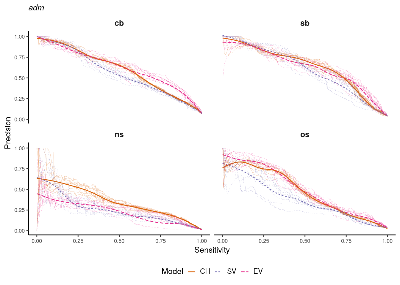
Figure 1.3: Precision-recall curves for adm district models. Bold lines indicate smoothed curves over 10 repeats. Faded lines indicate single repeats.
Concerning the ns class, the picture is quite different. The CH set outperforms both of the other sets almost over the complete value range. The EV set shows the lowest precision values at high rates of sensitivity, indicating that for this outcome class SV and EV predictors do not improve model performance. For the os class, the CH and EV sets almost perform identically. However, the EV set constantly achieves slightly higher precision values when sensitivity is above 0.5. The SV set performs substantially worse than the other predictor sets for sensitivity values between 0 and 0.7. Considering the bas representation for the outcome variable cb, CH and EV virtually show an identical performance (Figure 1.3). The SV predictor set obtains lower precision values for sensitivities between 0.3 to 0.9. Concerning the sb outcome variable, SV achieves higher precision than the other sets for low sensitivity values. Towards higher sensitivity, the CH set can maintain the highest precision while only slight differences exist between the SV and EV sets. Concerning the ns outcome variable, the pattern is similar to the one found for adm districts, indicating that the prediction of the ns outcome class does not benefit from more complex predictor sets. For os conflicts, similar to the adm representation, the EV set outperforms the other two sets almost over the complete value range. However, the difference to the CH set is only marginal, while SV achieves the lowest precision for increasing sensitivity values.
pr_data %>%
  filter(unit == "bas") %>%
  mutate(group = paste(type,var,rep,sep="-")) %>%
  select(-unit) %>%
  arrange(type,var,rep) %>%
  ggplot(aes(x=recall, y=precision, linetype=type, color=type)) +
  geom_smooth(aes(), alpha=1, size=.5, se=FALSE) +
  geom_line(aes(group=group), size=.1, alpha = .5) +
  scale_color_manual(values = RColorBrewer::brewer.pal(n=4, name  = "Dark2")[2:4]) +
  facet_wrap(~var, ncol = 2) +
  theme_classic() +
  labs(color = "Model", linetype = "Model", y = "Precision", x = "Sensitivity", subtitle = "bas") +
  guides(color=guide_legend(ncol=3, alpha=1)) +
  my_theme +
  theme(
    plot.subtitle =  element_markdown(size = 10, face =  "italic")
) 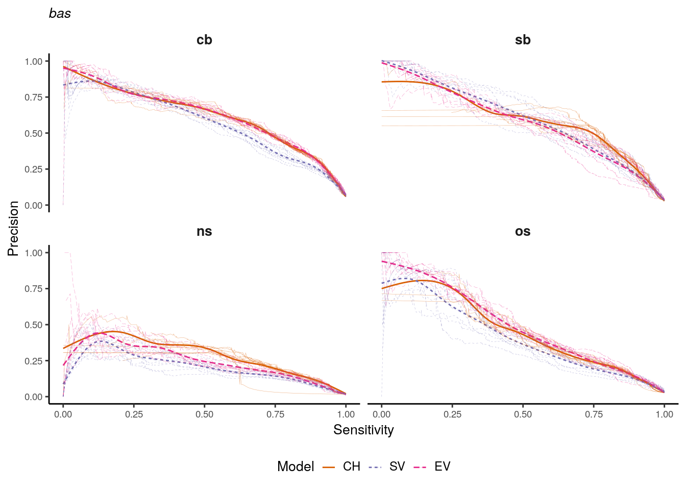
Figure 1.4: Precision-recall curves for bas district models. Bold lines indicate smoothed curves over 10 repeats. Faded lines indicate single repeats.
To summarize these findings, the EV set outperforms other model configurations for adm units for cb, sb, and os conflict classes. For the ns class, irrespective of the aggregation units, the CH set outperforms the other model configurations. Concerning the bas units, the EV set shows slightly better performance for the os class, but similar or worse performance to the CH set for all other classes. These findings do not support previous findings of a systematically increased performance of conflict prediction when environmental variables are included. The difference to models based only on conflict history is marginal, and the most simple model frequently outperforms complex variable configurations. However, the specific conflict class seems to play a role in how structural and environmental variables change conflict prediction performance. Specifically, the EV seems to improve the performance on the os outcome class as well as on cb and sb outcome classes for adm districts. It should be noted that the smoothed PR-curves do not represent the performance of a specific model, but the general tendency of a predictor set’s performance. The variance between the 10 repeats of training, however, can be quite high as indicated with previous results.
Despite their capability to easily compare different model configurations, PR-curves are not reported very often in related studies. Halkia et al. (2020) report distinct PR-curves for their 10-fold cross-validation strategy. Their results indicate that their model is more capable of achieving relatively high precision scores for increasing sensitivity which is in agreement with previous findings on the global performance. It underlines that the presented DL methods show weaker performance in terms of precision compared to related studies. The desirable feature of a model to maintain precision while increasing sensitivity is not observed at an equal level. Partly, this can be explained by the aggregation to country-months and differences in the definition of the conflict classes. However, comparing to existing conflict prediction tools reveals that it is possible to achieve a better balance between precision and sensitivity. Based on the selected predictor variables in this study, the models ability to reduce the False Positive Rate is limited compared to other studies. The deliberate exclusion of predictor variables delivering more context on the political and cultural compilation of a district could be a reason for the evident reduced performance in terms of precision of the proposed method. The results also illustrate the complexities in the field of conflict prediction. The focus of a machine learning procedure on one metric can adversely affect other performance metrics. It is essential to carefully select a metric for optimization, which represents the overall goal of the prediction task most closely. Because the costs associated with missing out on a conflict district-month are expected to be higher as the costs of wrongly predicting a conflict for a given district-month, the focus on the \(F_2\)-score mirrors this assumption. Optimizing towards it means putting more value on sensitivity which explains the reduced performance in terms of precision from a methodological point of view.
1.3 Temporal Performance
#files <- list.files("../output/acc/", pattern = ".rds", full.names = T)
files <- list.files("../output/test-results/", pattern = "test-results", full.names = T)
# files <- files[-grep("test-results-regression-basins", files)]
acc_data <- lapply(files, function(x){
  out <- vars_detect(x)
  tmp = readRDS(x)
  tmp$type = out$type

  tmp %>%
    filter(month != 0)
})
acc_data = do.call(rbind, acc_data)

acc_data %<>%
  mutate(var = factor(var, labels = c("all", "sb", "ns", "os"),
                      levels = c("all", "sb", "ns", "os")),
         type = factor(type,
                       labels = c("LR", "CH", "SV", "EV"),
                       levels = c("regression", "baseline", "structural", "environmental")),
         unit = if_else(unit == "basins", "bas", "adm"),
         unit = factor(unit, levels = c("adm", "bas"), labels = c("adm", "bas")))

labs.unit = c("_adm_", "_bas_")
names(labs.unit) = c("adm", "bas")
labs.var = c("__cb__", "__sb__", "__ns__", "__os__")
names(labs.var) = c("all", "sb", "ns", "os")
The occurrence of conflict is predicted 12 months into the future using a single threshold. Indications for the performance of different model configurations to distinguish between conflict and peace district-months irrespective of the time-dimension are given as density plots in the Appendix (Figures ?? to ??). Despite using a single cut-off value, the performance of the evaluated model is different along the months in the prediction horizon. Figure 1.5 depicts the obtained \(F_2\)-scores for both aggregation units considering each month in the prediction horizon individually. In general, the performance is relatively stable for most model configurations. Variations over time remain mostly subtle, but changes in both directions towards lower and higher scores are observed for the DL frameworks. The performance of the LR baseline deteriorates with an increasing prediction horizon for almost all conflict classes and is substantially lower compared to the DL models. For the outcome variable cb, a better performance of the SV and EV sets compared to the CH theme is observed for adm districts, though they almost perform identically. For bas districts, EV slightly outperforms all other themes over the entire horizon, but SV shows lower performance than CH. Better performances of the more complex predictor sets compared to the CH theme become more evident for the sb conflict class.
acc_data %>%
  filter(name == "f2") %>%
  dplyr::select(name, score, month, var, unit, type) %>%
  ggplot(aes(x=month, y=score, color=type, linetype=type))+
  stat_smooth(geom='line', alpha=.6, size=.5, se=FALSE, lwd=1)+
  facet_grid(unit~var, labeller = labeller(unit = labs.unit, var = labs.var)) +
  scale_x_continuous(breaks=c(1:12)) +
  ylim(0,1) +
  theme_classic() +
  scale_color_brewer(palette="Dark2") +
  labs(subtitle = "F2-score", x = "Prediction window (in months)", y = "Score", color = "Model", linetype = "Model") +
  guides(color=guide_legend(ncol=4)) +
  my_theme -> plt_out
plot_output(plt_out)
Figure 1.5: Time dependent performance of the F2-score for adm (top) and bas (bottom) districts. Single lines are obtained by smoothing over the individual scores obtained for 10 repeats.
For both aggregation units, the difference to the CH theme is more substantial over the complete prediction horizon. The pattern of the SV and EV theme over the prediction horizon is very similar and they perform equally well. Differences between adm and bas districts become evident for the ns class. Here the bas models almost show a monotonic increase in prediction performance over the horizon. The EV set overall achieves higher scores, especially after five months into the horizon. For adm districts, the CH theme outperforms the other predictor sets over the first half and towards the end of the horizon. Only for eight and nine months into the future, SV and EV achieve higher \(F_2\)-scores and then experience a substantial decrease in performance. For the os outcome class, the DL models perform equally well for the adm representation with a slightly better performance of the EV set. For bas districts, the increased performance of the EV is more pronounced, but towards the end of the horizon the difference compared to the SV set is reduced.
acc_data %>%
  filter(name == "aucpr") %>%
  dplyr::select(name, score, month, var, unit, type) %>%
  ggplot(aes(x=month, y=score, color=type, linetype=type))+
  stat_smooth(geom='line', alpha=.6, size=.5, se=FALSE, lwd=1)+
  facet_grid(unit~var, labeller = labeller(unit = labs.unit, var = labs.var)) +
  scale_x_continuous(breaks=c(1:12)) +
  ylim(0,1) +
  theme_classic() +
  scale_color_brewer(palette="Dark2") +
  labs(subtitle = "F2-score", x = "Prediction window (in months)", y = "Score", color = "Model", linetype = "Model") +
  guides(color=guide_legend(ncol=4)) +
  my_theme -> plt_out
plot_output(plt_out)
Figure 1.6: Time dependent performance of the AUPR metric. Single lines are obtained by smoothing over the individual scores obtained for 10 repeats.
In general, for the adm representation, the differences between the SV and EV sets are only marginal for all conflict class except ns, suggesting that environmental variables do not further increase the prediction performance. For the ns class, CH clearly shows some advantages over the other predictor sets for the most part of the prediction horizon, which is in agreement with previous findings. Considering the bas representation, EV outperforms other predictor sets except of the sb outcome class where the difference to the SV set is marginal. In contrast to adm districts, the performance compared to the CH theme is substantial, except for outcome class cb, suggesting that the selected predictor variables have a greater effect on prediction performance when they are aggregated on the bas districts.
acc_data %>%
  filter(name == "sensitivity") %>%
  dplyr::select(name, score, month, var, unit, type) %>%
  ggplot(aes(x=month, y=score, color=type, linetype=type))+
  stat_smooth(geom='line', alpha=.6, size=.5, se=FALSE, lwd=1)+
  facet_grid(unit~var, labeller = labeller(unit = labs.unit, var = labs.var)) +
  scale_x_continuous(breaks=c(1:12)) +
  ylim(0,1) +
  theme_classic() +
  scale_color_brewer(palette="Dark2") +
  labs(subtitle = "F2-score", x = "Prediction window (in months)", y = "Score", color = "Model", linetype = "Model") +
  guides(color=guide_legend(ncol=4)) +
  my_theme -> plt_out
plot_output(plt_out)
Figure 1.7: Time dependent performance of sensitivity. Single lines are obtained by smoothing over the individual scores obtained for 10 repeats.
Concerning the temporal performance measured by the AUPR, the general pattern is comparable to the one found for the \(F_2\)-score (Figure 1.5). We observe almost identical patterns for adm districts and outcome variables cb and sb. For outcome variables ns and os the higher performance of the CH is even more pronounced. Concerning the bas districts, the pattern is reversed and the differences of the SV and EV sets to the CH set is more strongly evident. For outcome variables cb and os, the EV set shows slightly higher performances than the SV set for the complete prediction horizon. The monotonic increase in performance of the ns outcome variable is not as clear, reaching a plateau after five months for the CH set and after eight months for the SV and EV sets.
Directly comparing model performances in terms of precision and sensitivity delivers an imperfect picture of the comparative performances between different model configurations. Rather than the absolute precision or sensitivity values, the balance between these metrics as expressed in the \(F_2\)-score or the AUPR better captures information on their mutual dependency. An alternative perspective to compare model performance in terms of precision and sensitivity is to analyze the “cost” a gain in one metric is associated with a loss in the other. An insightful distinction between adm and bas districts is found in this regard (Figure 1.7 & Figure 1.8). While the CH set initially delivers comparatively high values of sensitivity for adm districts, it is associated with higher precision values for bas districts. Increasing the complexity of the predictor variables with the SV set leads to a substantial decrease in sensitivity for adm districts but simultaneously increases the precision. For bas districts, moving to the SV set has the opposite effect of increasing the sensitivity but decreasing precision. Finally, the EV set achieves sensitivity and precision rates in between the CH and SV sets. These findings are in agreement with the results of the global performances. The EV theme is better capable of mediating between precision and recall for both aggregation districts. A distinction between the aggregation units is the direction from which this balance is achieved. Solely based on the CH set, adm districts seem beneficial to reach high sensitivity values. However, the predictions are associated with a high rate of false alarms because the precision is low. Using bas districts, CH delivers relatively high precision values, but the rate observed conflicts are detected remains low. This contrasting behavior could be harnessed to build early-warning systems with a specialized focus on precision or sensitivity. Some applications might emphasize the importance of detecting all future conflict district-months over the precision to only select relevant cases. The results suggest that such a case would benefit from a focus on adm districts. For cases where high precision is more relevant than selecting all future conflicts, a model based on bas districts could prove a valuable choice.
Concerning related studies, only Hegre et al. (2019) report time-dependent performance of their models. The prediction window differs from the one presented here, as they predict the occurrence of conflict for up to 36 months into the future. Additionally, they restrict their time-dependent performance analysis to the AUC and AUPR metrics. For the first 12 months, similar to the results presented here, the AUPR metric shows great stability for the country-month representation but with values above 0.90. For the grid representation, there is less stability and values as low as 0.35 are observed. Consistent with previous findings, the country-month data set can achieve substantially higher scores than the presented DL models. However, because the prediction window in this study has been set to 12 months only, the long-term performance can not be compared.
acc_data %>%
  filter(name == "precision") %>%
  dplyr::select(name, score, month, var, unit, type) %>%
  ggplot(aes(x=month, y=score, color=type, linetype=type))+
  stat_smooth(geom='line', alpha=.6, size=.5, se=FALSE, lwd=1)+
  facet_grid(unit~var, labeller = labeller(unit = labs.unit, var = labs.var)) +
  scale_x_continuous(breaks=c(1:12)) +
  ylim(0,1) +
  theme_classic() +
  scale_color_brewer(palette="Dark2") +
  labs(subtitle = "F2-score", x = "Prediction window (in months)", y = "Score", color = "Model", linetype = "Model") +
  guides(color=guide_legend(ncol=4)) +
  my_theme -> plt_out
plot_output(plt_out)
Figure 1.8: Time dependent performance of precision. Single lines are obtained by smoothing over the individual scores obtained for 10 repeats.
1.4 Spatial Performance
adm <- st_read("../data/vector/states_mask.gpkg", quiet = T)
adm <- select(adm, geom)
adm <- st_make_valid(adm)
bas <- st_read("../data/vector/basins_simple.gpkg", quiet = T)
bas <- select(bas, geom)
bas <- st_make_valid(bas)
crs <- st_crs("EPSG:3857")
adm <- st_transform(adm, crs)
adm <- st_simplify(adm, dTolerance = 1500, preserveTopology = T)
bas <- st_transform(bas, crs)
bas <- st_simplify(bas, dTolerance = 1000, preserveTopology = T)


files = list.files("../output/test-results/", pattern ="cnfrisk", full.names = T)

map_data = lapply(files, function(x){
  out = vars_detect(x)
  tmp = st_read(x, quiet = T)
  tmp = st_drop_geometry(tmp)
  tmp$unit = out$unit
  tmp$type = out$type
  tmp$var = out$var
  tmp %<>%
    select(unit,type,var,mean,obsv)
  if(out$unit == "basins") {
    st_as_sf(bind_cols(bas, tmp))
  } else {
    st_as_sf(bind_cols(adm, tmp))
  }
})

map_data = do.call(rbind, map_data)
The spatial dimension of the detection task is depicted for the outcome variable cb in Figures 1.9 and 1.10 for adm and bas districts, respectively. Additional maps for other outcome variables are found in the Appendix (Figures ?? to ??). In the upper left, the number of observed conflict months within the validation period from January to December 2019 is indicated. The other maps represent the averaged probability of conflict risk for the CH, SV, and EV theme, respectively. The most prominent patterns of high numbers of conflict occur in Mali, the cross border region of Lake Chad, within large parts of the Democratic Republic of Kongo (D.R. Kongo), the Southern part of Somalia, and the province of Cabo Delgado in Mozambique. Lower occurrences of conflict are observed in Libya, some regions in Algeria, Tunisia, Egypt, and larger areas in Sudan, South Sudan, and Ethiopia. Considering the distribution of the observed number of conflict months reveals that for both the adm and bas districts low numbers of conflict are more frequently observed. The number of districts experiencing 10 or more months of conflicts are increasing for both aggregation units. These observations indicate a general distinction between districts on the African continent. Some of them are characterized by intense and prolonged conflicts, such as Mali, D.R. Kongo or Somalia. Districts in their spatial neighborhood are characterized by relatively low numbers of conflicts so that a pattern of spatial clusters emerges. The majority of the continent does not show conflict events occurring at all within the testing year 2019.
The averaged probability of conflict reveals an interesting distinction between adm and bas districts. Considering the distribution of predicted probabilities, for adm districts, we can observe an increasing separation between peace and conflict district-months. For the CH theme, the probabilities are evenly distributed over the value range from 0.3 to 0.6 with a very high number of districts with a predicted conflict risk of approximately 0.35. Here, most districts without a recent conflict history have been labeled with this value. Districts with a prolonged conflict history are found towards the end of the value range. Moving to the SV theme, this separation becomes more evident, with a clear distinction of districts with a probability of conflict below and above 0.4. Here, virtually all districts within the Sahara and areas recently experiencing high-intensity conflicts such as Mali, the Kongo basin, and the region from Sudan to Somalia are characterized by higher conflict risks than the South and West African districts. Moving to the EV theme, the distinction between districts with a low probability of conflict becomes more pronounced.
map_data %>%
  filter(unit == "states", var == "all") -> plt_data

breaks = seq(0,1,0.1)

plt_data %>%
  filter(type == "baseline") %>%
  dplyr::select(obsv) %>%
  mutate(obsv = ifelse(obsv > 0, obsv, NA)) -> obsv_data

obsv_data %>%
  tm_shape() +
  tm_polygons("obsv",
              palette = "PuBu",
              lwd=.01,
              border.col = "grey90",
              breaks = 0:12,
              style = "fixed",
              title = "Conflict Months",
              showNA = FALSE,
              legend.hist = TRUE,
              labels = as.character(1:12)) +
  tm_legend(stack = "horizontal") +
  tm_layout(title = "Observation",
            title.position = c("right", "top"),
            title.size = 0.7,
            legend.title.size = 0.7,
            legend.text.size = 0.45,
            legend.position = c("left", "bottom"),
            legend.outside.position = "bottom",
            legend.bg.color = "white",
            legend.bg.alpha = 0,
            legend.outside = TRUE,
            legend.hist.width = 1,
            legend.hist.height = .8,
            legend.hist.size = .5)   -> map_obsv

plt_data %>%
  filter(type == "baseline") %>%
  tm_shape() +
  tm_polygons("mean",
              palette = "PuBu",
              lwd=.01,
              border.col = "grey90",
              title = "Probability of conflict",
              breaks = breaks,
              style = "fixed",
              legend.hist = TRUE) +
  tm_legend(stack = "horizontal") +
  tm_layout(title = "Conflict History (CH)",
            title.position = c("right", "top"),
            title.size = 0.7,
            legend.title.size = 0.7,
            legend.text.size = 0.45,
            legend.position = c("left", "bottom"),
            legend.outside.position = "bottom",
            legend.bg.color = "white",
            legend.bg.alpha = 0,
            legend.outside = TRUE,
            legend.hist.width = 1,
            legend.hist.height = .8,
            legend.hist.size = .5)   -> map_bas

plt_data %>%
  filter(type == "structural") %>%
  tm_shape() +
  tm_polygons("mean",
              palette = "PuBu",
              lwd=.01,
              border.col = "grey90",
              title = "Probability of conflict",
              breaks = breaks,
              style = "fixed",
              legend.hist = TRUE)  +
  tm_legend(stack = "horizontal") +
  tm_layout(title = "Structural Variables (SV)",
            title.position = c("right", "top"),
            title.size = 0.7,
            legend.title.size = 0.7,
            legend.text.size = 0.45,
            legend.position = c("left", "bottom"),
            legend.outside.position = "bottom",
            legend.bg.color = "white",
            legend.bg.alpha = 0,
            legend.outside = TRUE,
            legend.hist.width = 1,
            legend.hist.height = .8,
            legend.hist.size = .5)  -> map_str

plt_data %>%
  filter(type == "environmental") %>%
  tm_shape() +
  tm_polygons("mean",
              palette = "PuBu",
              lwd=.01,
              border.col = "grey90",
              title = "Probability of conflict",
              breaks = breaks,
              style = "fixed",
              legend.hist = TRUE)  +
  tm_legend(stack = "horizontal") +
  tm_layout(title = "Environmental Variables (EV)",
            title.position = c("right", "top"),
            title.size = 0.7,
            legend.title.size = 0.7,
            legend.text.size = 0.45,
            legend.position = c("left", "bottom"),
            legend.outside.position = "bottom",
            legend.bg.color = "white",
            legend.bg.alpha = 0,
            legend.outside = TRUE,
            legend.hist.width = 1,
            legend.hist.height = .8,
            legend.hist.size = .5)  -> map_env

tmap_arrange(map_obsv, map_bas, map_str, map_env, ncol = 2)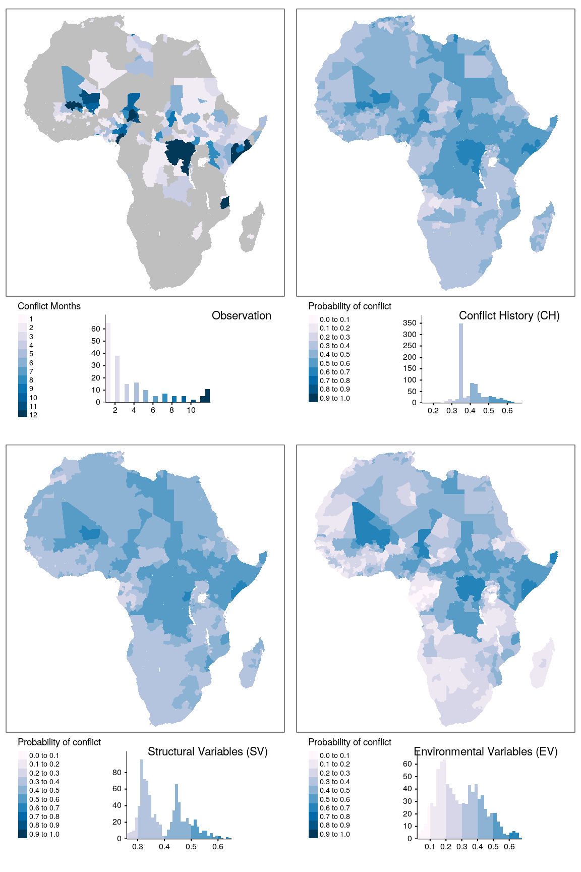
Figure 1.9: Spatial prediction of conflict class cb for adm districts. Observed conflict occurrences (upper left) and averaged probabilities of conflict. Grey polygons indicate zero occurrences of conflict.
For example, large parts of Namibia are attributed to a lower risk of conflict than districts in South Africa, Zambia, and Angola. This indicates that the model evaluates these regions differently, distinguishing between very low and slightly elevated conflict risks. For the other model configurations, these differences are not as apparent. On the other end of the value range, areas already experiencing ongoing conflicts are now more frequently associated with probability values above 0.6, rendering these very high conflict risk areas more distinguishable from the general elevated conflict risk in their neighborhood. For bas units, the pattern is strikingly different considering the SV theme. Here, the differentiation between low-risk districts and districts with an elevated risk is heavily pronounced. A similar pattern emerges when one considers the densitiy distribution of predicted conflict probability of peace versus conflict district months (Figures ?? to ??). The SV theme for bas districts seems to be very capable of distinguishing between districts with low and elevated conflict risk. The majority of districts are associated with predicted probabilities about 0.1, while the major conflict zones are associated with values of 0.4 and higher. This capability of the SV theme is a desirable property of a conflict prediction model. Unfortunately, this discriminatory power is not observed on the same level for the EV theme. Here, we can observe a similar pattern as with the adm districts distinguishing between districts with very low conflict risks and districts with slightly elevated conflict risk. However, the pattern for districts with more elevated risk is not as straightforward since most districts are associated with moderate probabilities between 0.3 and 0.4. The zones with a recent intense conflict history still show elevated conflict risks. However, their differentiation against their neighborhood is less pronounced compared to the SV theme.
Because their model is being used as an early-warning system, Hegre et al. (2019) present their conflict forecast as spatial maps based on a country basis and a grid indicating the risk of conflicts expressed as a percentage. They jointly use both prediction patterns first to identify countries at a high risk of conflict and then pinpoint areas with high conflict risk more accurately. While this approach seems reasonable to sequentially achieve higher spatial accuracy, it should be kept in mind that the grid-based performance is substantially lower and associated with high uncertainty. However, they do not spatially compare their prediction results to observed conflicts in a held-out validation set.
map_data %>%
  filter(unit == "basins", var == "all") -> plt_data

breaks = seq(0,1,0.1)

plt_data %>%
  filter(type == "baseline") %>%
  dplyr::select(obsv) %>%
  mutate(obsv = ifelse(obsv > 0, obsv, NA)) -> obsv_data

obsv_data %>%
  tm_shape() +
  tm_polygons("obsv",
              palette = "PuBu",
              lwd=.01,
              border.col = "grey90",
              breaks = 0:12,
              style = "fixed",
              title = "Conflict Months",
              showNA = FALSE,
              legend.hist = TRUE,
              labels = as.character(1:12)) +
  tm_legend(stack = "horizontal") +
  tm_layout(title = "Observation",
            title.position = c("right", "top"),
            title.size = 0.7,
            legend.title.size = 0.7,
            legend.text.size = 0.45,
            legend.position = c("left", "bottom"),
            legend.outside.position = "bottom",
            legend.bg.color = "white",
            legend.bg.alpha = 0,
            legend.outside = TRUE,
            legend.hist.width = 1,
            legend.hist.height = .8,
            legend.hist.size = .5)     -> map_obsv

plt_data %>%
  filter(type == "baseline") %>%
  tm_shape() +
  tm_polygons("mean",
              palette = "PuBu",
              lwd=.01,
              border.col = "grey90",
              title = "Probability of conflict",
              breaks = breaks,
              style = "fixed",
              legend.hist = TRUE) +
  tm_legend(stack = "horizontal") +
  tm_layout(title = "Conflict History (CH)",
            title.position = c("right", "top"),
            title.size = 0.7,
            legend.title.size = 0.7,
            legend.text.size = 0.45,
            legend.position = c("left", "bottom"),
            legend.outside.position = "bottom",
            legend.bg.color = "white",
            legend.bg.alpha = 0,
            legend.outside = TRUE,
            legend.hist.width = 1,
            legend.hist.height = .8,
            legend.hist.size = .5)   -> map_bas

plt_data %>%
  filter(type == "structural") %>%
  tm_shape() +
  tm_polygons("mean",
              palette = "PuBu",
              lwd=.01,
              border.col = "grey90",
              title = "Probability of conflict",
              breaks = breaks,
              style = "fixed",
              legend.hist = TRUE)  +
  tm_legend(stack = "horizontal") +
  tm_layout(title = "Structural Variables (SV)",
            title.position = c("right", "top"),
            title.size = 0.7,
            legend.title.size = 0.7,
            legend.text.size = 0.45,
            legend.position = c("left", "bottom"),
            legend.outside.position = "bottom",
            legend.bg.color = "white",
            legend.bg.alpha = 0,
            legend.outside = TRUE,
            legend.hist.width = 1,
            legend.hist.height = .8,
            legend.hist.size = .5)  -> map_str

plt_data %>%
  filter(type == "environmental") %>%
  tm_shape() +
  tm_polygons("mean",
              palette = "PuBu",
              lwd=.01,
              border.col = "grey90",
              title = "Probability of conflict",
              breaks = breaks,
              style = "fixed",
              legend.hist = TRUE)  +
  tm_legend(stack = "horizontal") +
  tm_layout(title = "Environmental Variables (EV)",
            title.position = c("right", "top"),
            title.size = 0.7,
            legend.title.size = 0.7,
            legend.text.size = 0.45,
            legend.position = c("left", "bottom"),
            legend.outside.position = "bottom",
            legend.bg.color = "white",
            legend.bg.alpha = 0,
            legend.outside = TRUE,
            legend.hist.width = 1,
            legend.hist.height = .8,
            legend.hist.size = .5)  -> map_env

tmap_arrange(map_obsv, map_bas, map_str, map_env, ncol = 2)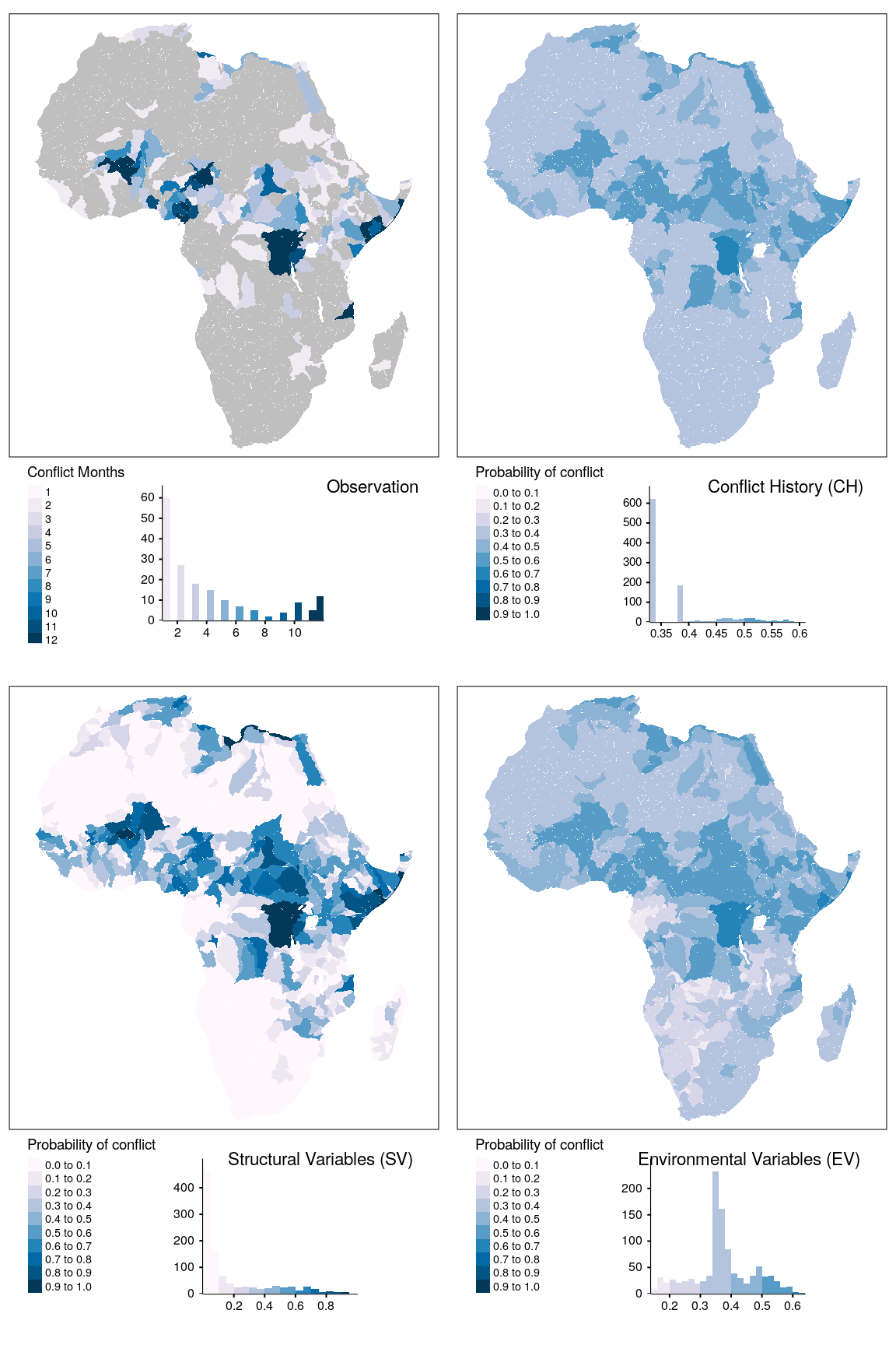
Figure 1.10: Spatial prediction of conflict class cb for bas districts. Observed conflict occurrences (upper left) and averaged probabilities of conflict. Grey polygons indicate zero occurrences of conflict.
A scientific publication analyzing the actual prediction for the year 2019 is still in the press as of the time of writing this thesis. Kuzma et al. (2020), although providing their prediction results as a map of conflict risk to the broader public (https://waterpeacesecurity.org/map), do not compare their prediction against actual observations in space. Halkia et al. (2020) deliver a map indicating the number of false positives and negatives between 1989 and 2013. Their results show a concentration of false negatives in East Africa as well as in parts of Southern Africa for subnational conflicts. For national power conflicts, these concentrations are found in East and West Africa. Overall, though most related studies serve the purpose of informing decision-makers on the potential spatiotemporal occurrence, the spatial dimension of these predictions is not thoroughly discussed in their respective scientific communication rendering more elaborated comparisons unfeasible.
1.5 Analysis of Variance
Since Leven’s test for the homogeneity of variance revealed a statistically significant difference in variance between groups violating the assumption for ANOVA. For this reason, both normal distribution and variance were visually cross-checked (Figures ?? & ??). While the assumption of normal distribution holds for the visual interpretation, differences in variance were observed, especially for the LR model versus the DL models. For that reason, the non-parametric Welch-James test was applied to the interaction term between aggregation unit and predictor set (Table 1.2).
files <- list.files("../output/test-results/", pattern = "test-results", full.names = T)
acc_data <- lapply(files, function(x){
  out <- vars_detect(x)
  tmp = readRDS(x)
  tmp %<>%
    filter(name == "f2",
           month == 0)
  tmp$type = out$type
  tmp
})

acc_data = do.call(rbind, acc_data)
acc_data %<>%
  mutate(type = factor(type,
                       levels = c("regression", "baseline", "structural", "environmental"),
                       labels = c("LR", "CH", "SV", "EV")),
         var = factor(var,
                      levels = c("all", "sb", "ns", "os"),
                      labels = c("cb", "sb", "ns", "os")),
         unit = factor(unit,
                       levels = c("states", "basins"),
                       labels = c("adm", "bas")))
#%>% filter(type != "LR")


# # boxplot
# ggboxplot(acc_data, y = "score", x = "type", color = "unit") +
#   facet_wrap(~var)
#
# # # check for outliers
# acc_data %>%
#   group_by(var) %>%
#   identify_outliers(score)
# # -> no extreme outliers detected
#
# # calculate linear models
# acc_data %>%
#   group_by(var) %>%
#   nest() %>%
#   mutate(model = map(data, ~lm(score ~ unit + type + unit*type, data = .x))) -> lm_models
#
# # check for normal distribution
# lm_models %>%
#   mutate(residuals = map(model, residuals)) %>%
#   select(var, residuals) %>%
#   mutate(shapiro = map(residuals, shapiro_test)) %>%
#   select(-residuals) %>%
#   unnest(shapiro)

# -> normality is slightly violated for some groups

# use levene test to check for homogenous variance
# acc_data %>%
#   group_by(var) %>%
#   levene_test(score ~ interaction(unit,type)) %>%
#   mutate(sig = if_else(p > 0.1, "No", "Yes"))
#
# acc_data %>%
#   group_by(var) %>%
#   levene_test(score ~ unit) %>%
#   mutate(sig = if_else(p > 0.1, "No", "Yes"))
#
# acc_data %>%
#   group_by(var) %>%
#   levene_test(score ~ type) %>%
#   mutate(sig = if_else(p > 0.1, "No", "Yes"))
# variance assumption does not hold

acc_data %>%
  group_by(var) %>%
  nest() %>%
  mutate(
    welch = map(data, ~welchADF.test(score ~ unit*type, data = .x)),
  ) %>%
  select(-data) -> test_results

welch_anova = do.call(rbind,lapply(1:nrow(test_results), function(i){
  tmp = test_results$welch[[i]]
  unit.p = tmp$unit$pval
  type.p = tmp$type$pval
  ut.p = tmp$`unit:type`$pval
  var = test_results$var[i]
  tibble(var = var, p = c(unit.p,type.p,ut.p), term = c("unit", "type", "unit:type"))
}))


welch_anova %>%
  mutate(
    sig = if_else(p>0.05, "", "*"),
    sig = if_else(p<0.01, "**", sig),
    sig = if_else(p<0.001, "***", sig),
    p = formatC(p, format = "e", digits = 2),
  ) %>%
  select(var, term, p, sig) %>%
  pivot_wider(id_cols = c(1,2), names_from = var, values_from = 3:4) %>%
  select(1,2,6,5,9,3,7,4,8) %>%
  thesis_kable(align = c(rep("l", 9)),
               linesep = c(""),
               escape = F,
               col.names = c("Term",rep(c("p", "Sig."), 4)),
               longtable = T,
               caption = c("Results of the Welch-James ANOVA.")
  ) %>%
  kable_styling(latex_options = "HOLD_position", font_size = 8) %>%
  add_header_above(c(" ", "cb" = 2, "sb" = 2, "ns" = 2, "os"= 2), bold = T) %>%
  footnote(general = "The significance level is indicated according to: *p\\\\textless0.05, **p\\\\textless0.01, ***p\\\\textless0.001",
           threeparttable = T,
           escape = FALSE,
           general_title = "General:",
footnote_as_chunk = T)| Term | p | Sig. | p | Sig. | p | Sig. | p | Sig. |
|---|---|---|---|---|---|---|---|---|
| unit | 0.00e+00 | *** | 1.77e-03 | ** | 3.65e-01 | 2.41e-08 | *** | |
| type | 0.00e+00 | *** | 0.00e+00 | *** | 0.00e+00 | *** | 0.00e+00 | *** |
| unit:type | 3.77e-05 | *** | 2.70e-03 | ** | 1.89e-02 |
|
6.70e-04 | *** |
| General: The significance level is indicated according to: p\textless0.05, p\textless0.01, p\textless0.001 |
From Table 1.2 it becomes evident that the interaction terms between aggregation unit and predictor set are highly significant on the for outcome variables cb, sb, and os. For ns we find significant differences in the group’s mean at the 95 % confidence interval. Because all interaction terms indicate a significant difference, in the following, a discussion of the main effects will be omitted. For reasons of brevity, only the interaction terms for the contrast of the EV predictor set against all over sets will be discussed as it is also the most relevant contrast to answer H1 and H2.
acc_data %>%
  mutate(inter = interaction(unit, type)) %>%
  group_by(var) %>%
  games_howell_test(score ~ inter) %>%
  mutate(type1 = str_sub(group1, 5,6),
         type2 = str_sub(group2, 5,6),
         unit1 = str_sub(group1, 1,3),
         unit2 = str_sub(group2, 1,3)) %>%
  filter(str_detect(group2, "EV")) %>%
  mutate(type1 = factor(type1,
                        levels = c("LR", "CH", "SV", "EV")),
         type2 = factor(type2,
                        levels = c("LR", "CH", "SV", "EV")),
         unit1 = factor(unit1,
                        levels = c("adm", "bas")),
         unit2 = factor(unit2,
                        levels = c("adm", "bas"))) %>%
  arrange(var, type1, unit2) %>%
  select(var, estimate, p = p.adj, type1, type2, unit1, unit2) %>%
  mutate(
    sig = if_else(p>0.05, "", "*"),
    sig = if_else(p<0.01, "**", sig),
    sig = if_else(p<0.001, "***", sig),
    estimate = round(estimate,5),
    contrast = paste(unit2,unit1,sep=":"),
    p = formatC(p, format = "e", digits = 1),
    sig = if_else(sig == "", p, paste0(p, sig))
  ) %>%
  select(var, unit2, unit1, type1, contrast, estimate, sig) %>%
  pivot_wider(id_cols = c(4:5), values_from = c(2:3,6:7), names_from = 1) %>%
  select(contrast,
         unit1_cb, unit2_cb,
         estimate_cb, sig_cb,
         estimate_sb, sig_sb,
         estimate_ns, sig_ns,
         estimate_os, sig_os
  ) -> table_data


table_data %>%
  select(-c(unit1_cb, unit2_cb)) %>%
  thesis_kable(align = c(rep("l", 13)),
               linesep = c(""),
               escape = F,
               col.names = c("Contrast",rep(c("Est.", "p"), 4)),
               longtable = T,
               style = list(latex_options = "HOLD_position", font_size = 8),
               caption = c('Results of the Games-Howell test for difference in mean values.')
  ) %>%
  group_rows("EV:LR", 1, 4) %>%
  group_rows("EV:CH", 5, 8) %>%
  group_rows("EV:SV", 9, 12) %>%
  group_rows("EV:EV", 13, 13) %>%
  add_header_above(c(" ", "cb" = 2, "sb" = 2, "ns" = 2, "os" = 2), bold = T) %>%
  footnote(general = 'Contrasts are indicated by ":" reading as the left-hand side compared to the right-hand side. Est. indicates the difference in mean, p indicates the p value with significance level according to: *p\\\\textless0.05, **p\\\\textless0.01, ***p\\\\textless0.001',
           threeparttable = T,
           escape = FALSE,
           general_title = "General:",
footnote_as_chunk = T)| Contrast | Est. | p | Est. | p | Est. | p | Est. | p |
|---|---|---|---|---|---|---|---|---|
| EV:LR | ||||||||
| adm:adm | 0.29299 | 2.4e-10*** | 0.40543 | 4.6e-10*** | 0.25543 | 7.1e-08*** | 0.28137 | 1.4e-10*** |
| adm:bas | 0.22865 | 3.1e-10*** | 0.34574 | 7.9e-10*** | 0.22216 | 3.0e-07*** | 0.22065 | 0.0e+00*** |
| bas:adm | 0.36458 | 9.9e-12*** | 0.42837 | 3.4e-10*** | 0.30397 | 3.7e-10*** | 0.32709 | 2.2e-10*** |
| bas:bas | 0.30024 | 9.4e-11*** | 0.36869 | 3.9e-10*** | 0.27070 | 3.1e-10*** | 0.26636 | 5.3e-11*** |
| EV:CH | ||||||||
| adm:adm | 0.02770 | 1.2e-01 | 0.04354 | 2.1e-01 | -0.02863 | 7.7e-01 | 0.02135 | 2.1e-01 |
| adm:bas | -0.04619 | 4.9e-06*** | 0.04032 | 8.4e-01 | 0.06320 | 6.6e-01 | 0.00803 | 1.0e+00 |
| bas:adm | 0.09929 | 7.8e-06*** | 0.06649 | 1.6e-02* | 0.01991 | 8.6e-01 | 0.06706 | 1.6e-05*** |
| bas:bas | 0.02540 | 3.0e-03** | 0.06327 | 4.1e-01 | 0.11175 | 1.1e-01 | 0.05374 | 2.5e-02* |
| EV:SV | ||||||||
| adm:adm | 0.00130 | 1.0e+00 | 0.01441 | 8.7e-01 | 0.04002 | 8.6e-01 | 0.01428 | 7.6e-01 |
| adm:bas | -0.03179 | 5.5e-04*** | -0.02382 | 4.8e-01 | -0.01401 | 9.6e-01 | -0.01023 | 9.8e-01 |
| bas:adm | 0.07289 | 2.0e-11*** | 0.03736 | 1.9e-02* | 0.08856 | 1.1e-01 | 0.06000 | 3.4e-04*** |
| bas:bas | 0.03980 | 5.9e-05*** | -0.00087 | 1.0e+00 | 0.03453 | 1.0e-02* | 0.03549 | 1.1e-01 |
| EV:EV | ||||||||
| bas:adm | 0.07159 | 3.4e-11*** | 0.02295 | 4.0e-01 | 0.04854 | 4.0e-02* | 0.04571 | 8.7e-06*** |
| General: Contrasts are indicated by “:” reading as the left-hand side compared to the right-hand side. Est. indicates the difference in mean, p indicates the p value with significance level according to: p\textless0.05, p\textless0.01, p\textless0.001 | ||||||||
First, the contrast between the EV to the LR models sets will be considered. Consistently for all outcome variables and aggregation units, the EV models achieve substantial higher \(F_2\)-scores between 0.221 and 0.428 at a highly significant level. The greatest differences are observed for the contrast between the bas districts compared to adm districts. Moving to the comparison between the EV and CH sets, there are no significant differences in the mean \(F_2\)-scores for contrasting adm districts across all outcome variables. This indicates that for adm districts, environmental predictors do not increase model performance compared to the models containing the conflict history alone. Also, for the cb outcome variable, the EV set for adm districts achieves a lower performance compared to the CH bas model. For the outcome classes cb and os, bas districts on average achieve 0.1 and 0.067 higher \(F_2\)-scores compared to adm districts, respectively. For the outcome variable sb, the difference in mean is comparable but less significant. For ns no significant differences are observed. Considering the contrast between bas models, only for cb and os we observe higher average \(F_2\)-scores on a significant level, indicating that for sb and os including environmental predictors does not improve model performance.
This finding is supported by the contrast between EV and SV predictor sets. Again, considering only adm districts, no significant differences are found and in comparison to bas districts they achieve lower \(F_2\)-scores on average. Higher averages are found for bas districts compared to adm districts for cb, sb, and os outcome classes on a significant level but not for ns. Considering the contrasts for bas districts, only for the cb outcome class we observe a higher score moving from the SV to the EV set in the amount of 0.04 points in \(F_2\)-score. For all other outcome variables, including environmental predictors does not further improve performance further. Comparing the EV sets for bas with adm districts reveals that except for outcome class sb significantly higher mean values are observed for bas districts.
The presented evidence in terms of the analysis of variance is consistent with the visualization in Figure 1.1, where bas districts are characterized with higher \(F_2\)-scores compared to adm districts. However, the variance of the CH set for bas districts is substantially larger for sb and ns outcome classes which explains the insignificant findings for these classes.
Based on these results, H1, which states that environmental variables significantly increase the model performance, can only be confirmed considering outcome variables cb in combination with bas districts where a significant difference of 0.025 points in \(F_2\)-score is observed between the CH and EV set. For all other outcome variables and especially for adm districts, no significant increases in mean moving from the CH to the SV and EV predictor sets were observed. Concerning H2, stating that bas districts can achieve better performance than adm districts, the results generally indicate a confirmation of the hypothesis except for the sb and ns outcome class where no significant differences in the mean are observed. Considering the cb outcome class, the differences are found to be between 0.072 and 0.099 on a significant level based on the EV comparison. For the outcome class os, slightly lower mean differences between 0.046 and 0.067 are found.
2 References
Breiman, L., 2001. Random forests. Machine learning 45, 5–32. https://doi.org/10.1023/A:1010933404324
Collier, P., 1998. On economic causes of civil war. Oxford Economic Papers 50, 563–573. https://doi.org/10.1093/oep/50.4.563
Cooney, C., Korik, A., Folli, R., Coyle, D., 2020. Evaluation of Hyperparameter Optimization in Machine and Deep Learning Methods for Decoding Imagined Speech EEG. Sensors 20, 4629. https://doi.org/10.3390/s20164629
Eck, K., Hultman, L., 2007. One-Sided Violence Against Civilians in War: Insights from New Fatality Data. Journal of Peace Research 44, 233–246. https://doi.org/10.1177/0022343307075124
Halkia, M., Ferri, S., Schellens, M.K., Papazoglou, M., Thomakos, D., 2020. The Global Conflict Risk Index: A quantitative tool for policy support on conflict prevention. Progress in Disaster Science 6, 100069. https://doi.org/10.1016/j.pdisas.2020.100069
Hegre, H., Allansson, M., Basedau, M., Colaresi, M., Croicu, M., Fjelde, H., Hoyles, F., Hultman, L., Högbladh, S., Jansen, R., Mouhleb, N., Muhammad, S.A., Nilsson, D., Nygård, H.M., Olafsdottir, G., Petrova, K., Randahl, D., Rød, E.G., Schneider, G., von Uexkull, N., Vestby, J., 2019. ViEWS: A political violence early-warning system. Journal of Peace Research 56, 155–174. https://doi.org/10.1177/0022343319823860
Kuzma, S., Kerins, P., Saccoccia, E., Whiteside, C., Roos, H., Iceland, C., 2020. Leveraging Water Data in a Machine Learning-Based Model for Forecasting Violent Conflict. Technical note. [WWW Document]. URL https://www.wri.org/publication/leveraging-water-data
Lin, T.-Y., Goyal, P., Girshick, R., He, K., Doll’ar, P., 2018. Focal Loss for Dense Object Detection. arXiv:1708.02002 [cs].
Probst, P., Boulesteix, A.-L., 2018. To Tune or Not to Tune the Number of Trees in Random Forest. Journal of Machine Learning Research 18.
Schellens, M.K., Belyazid, S., 2020. Revisiting the Contested Role of Natural Resources in Violent Conflict Risk through Machine Learning. Sustainability 12, 6574. https://doi.org/10.3390/su12166574
Sundberg, R., Eck, K., Kreutz, J., 2012. Introducing the UCDP Non-State Conflict Dataset. Journal of Peace Research 49, 351–362. https://doi.org/10.1177/0022343311431598
Zhang, Y., Wallace, B., 2016. A Sensitivity Analysis of (and Practitioners Guide to) Convolutional Neural Networks for Sentence Classification. arXiv:1510.03820 [cs].
sessionInfo()R version 3.6.3 (2020-02-29)
Platform: x86_64-pc-linux-gnu (64-bit)
Running under: Debian GNU/Linux 10 (buster)
Matrix products: default
BLAS/LAPACK: /usr/lib/x86_64-linux-gnu/libopenblasp-r0.3.5.so
locale:
[1] LC_CTYPE=en_US.UTF-8 LC_NUMERIC=C
[3] LC_TIME=en_US.UTF-8 LC_COLLATE=en_US.UTF-8
[5] LC_MONETARY=en_US.UTF-8 LC_MESSAGES=C
[7] LC_PAPER=en_US.UTF-8 LC_NAME=C
[9] LC_ADDRESS=C LC_TELEPHONE=C
[11] LC_MEASUREMENT=en_US.UTF-8 LC_IDENTIFICATION=C
attached base packages:
[1] stats graphics grDevices utils datasets methods base
other attached packages:
[1] plotly_4.9.2.1 lubridate_1.7.9.2 rgdal_1.5-18 countrycode_1.2.0
[5] welchADF_0.3.2 rstatix_0.6.0 ggpubr_0.4.0 scales_1.1.1
[9] RColorBrewer_1.1-2 latex2exp_0.4.0 cubelyr_1.0.0 gridExtra_2.3
[13] ggtext_0.1.1 magrittr_2.0.1 tmap_3.2 sf_0.9-7
[17] raster_3.4-5 sp_1.4-4 forcats_0.5.0 stringr_1.4.0
[21] purrr_0.3.4 readr_1.4.0 tidyr_1.1.2 tibble_3.0.6
[25] tidyverse_1.3.0 huwiwidown_0.0.1 kableExtra_1.3.1 knitr_1.31
[29] rmarkdown_2.7.3 bookdown_0.21 ggplot2_3.3.3 dplyr_1.0.2
[33] devtools_2.3.2 usethis_2.0.0
loaded via a namespace (and not attached):
[1] readxl_1.3.1 backports_1.2.0 workflowr_1.6.2
[4] lwgeom_0.2-5 lazyeval_0.2.2 splines_3.6.3
[7] crosstalk_1.1.0.1 leaflet_2.0.3 digest_0.6.27
[10] htmltools_0.5.1.1 memoise_1.1.0 openxlsx_4.2.3
[13] remotes_2.2.0 modelr_0.1.8 prettyunits_1.1.1
[16] colorspace_2.0-0 rvest_0.3.6 haven_2.3.1
[19] xfun_0.21 leafem_0.1.3 callr_3.5.1
[22] crayon_1.4.0 jsonlite_1.7.2 lme4_1.1-26
[25] glue_1.4.2 stars_0.4-3 gtable_0.3.0
[28] webshot_0.5.2 car_3.0-10 pkgbuild_1.2.0
[31] abind_1.4-5 DBI_1.1.0 Rcpp_1.0.5
[34] viridisLite_0.3.0 gridtext_0.1.4 units_0.6-7
[37] foreign_0.8-71 htmlwidgets_1.5.3 httr_1.4.2
[40] ellipsis_0.3.1 farver_2.0.3 pkgconfig_2.0.3
[43] XML_3.99-0.3 dbplyr_2.0.0 labeling_0.4.2
[46] tidyselect_1.1.0 rlang_0.4.10 later_1.1.0.1
[49] tmaptools_3.1 munsell_0.5.0 cellranger_1.1.0
[52] tools_3.6.3 cli_2.3.0 generics_0.1.0
[55] broom_0.7.2 evaluate_0.14 yaml_2.2.1
[58] processx_3.4.5 leafsync_0.1.0 fs_1.5.0
[61] zip_2.1.1 nlme_3.1-150 xml2_1.3.2
[64] compiler_3.6.3 rstudioapi_0.13 curl_4.3
[67] png_0.1-7 e1071_1.7-4 testthat_3.0.1
[70] ggsignif_0.6.0 reprex_0.3.0 statmod_1.4.35
[73] stringi_1.5.3 highr_0.8 ps_1.5.0
[76] desc_1.2.0 lattice_0.20-41 Matrix_1.2-18
[79] markdown_1.1 nloptr_1.2.2.2 classInt_0.4-3
[82] vctrs_0.3.6 pillar_1.4.7 lifecycle_0.2.0
[85] data.table_1.13.2 httpuv_1.5.5 R6_2.5.0
[88] promises_1.1.1 KernSmooth_2.23-18 rio_0.5.16
[91] sessioninfo_1.1.1 codetools_0.2-16 dichromat_2.0-0
[94] boot_1.3-25 MASS_7.3-53 assertthat_0.2.1
[97] pkgload_1.1.0 rprojroot_2.0.2 withr_2.4.1
[100] mgcv_1.8-33 parallel_3.6.3 hms_1.0.0
[103] grid_3.6.3 minqa_1.2.4 class_7.3-17
[106] carData_3.0-4 git2r_0.27.1 base64enc_0.1-3