Mapping
Jens Daniel Müller
21 August, 2020
Last updated: 2020-08-21
Checks: 7 0
Knit directory: Cant_eMLR/
This reproducible R Markdown analysis was created with workflowr (version 1.6.2). The Checks tab describes the reproducibility checks that were applied when the results were created. The Past versions tab lists the development history.
Great! Since the R Markdown file has been committed to the Git repository, you know the exact version of the code that produced these results.
Great job! The global environment was empty. Objects defined in the global environment can affect the analysis in your R Markdown file in unknown ways. For reproduciblity it’s best to always run the code in an empty environment.
The command set.seed(20200707) was run prior to running the code in the R Markdown file. Setting a seed ensures that any results that rely on randomness, e.g. subsampling or permutations, are reproducible.
Great job! Recording the operating system, R version, and package versions is critical for reproducibility.
Nice! There were no cached chunks for this analysis, so you can be confident that you successfully produced the results during this run.
Great job! Using relative paths to the files within your workflowr project makes it easier to run your code on other machines.
Great! You are using Git for version control. Tracking code development and connecting the code version to the results is critical for reproducibility.
The results in this page were generated with repository version 0026e0d. See the Past versions tab to see a history of the changes made to the R Markdown and HTML files.
Note that you need to be careful to ensure that all relevant files for the analysis have been committed to Git prior to generating the results (you can use wflow_publish or wflow_git_commit). workflowr only checks the R Markdown file, but you know if there are other scripts or data files that it depends on. Below is the status of the Git repository when the results were generated:
Ignored files:
    Ignored:    .Rproj.user/
    Ignored:    data/GLODAPv1_1/
    Ignored:    data/GLODAPv2_2016b_MappedClimatologies/
    Ignored:    data/GLODAPv2_2020/
    Ignored:    data/Gruber_2019/
    Ignored:    data/WOCE/
    Ignored:    data/World_Ocean_Atlas_2013_Clement/
    Ignored:    data/World_Ocean_Atlas_2018/
    Ignored:    data/eMLR/
    Ignored:    data/mapping/
    Ignored:    data/pCO2_atmosphere/
    Ignored:    dump/
    Ignored:    figure/
Note that any generated files, e.g. HTML, png, CSS, etc., are not included in this status report because it is ok for generated content to have uncommitted changes.
These are the previous versions of the repository in which changes were made to the R Markdown (analysis/mapping.Rmd) and HTML (docs/mapping.html) files. If you’ve configured a remote Git repository (see ?wflow_git_remote), click on the hyperlinks in the table below to view the files as they were in that past version.
| File | Version | Author | Date | Message |
|---|---|---|---|---|
| Rmd | 0026e0d | jens-daniel-mueller | 2020-08-21 | Switch back to WOA18 |
| html | af0bf7c | jens-daniel-mueller | 2020-08-21 | Build site. |
| Rmd | d4ffb66 | jens-daniel-mueller | 2020-08-21 | Switch back to WOA13 gamma from Clement |
| html | d514413 | jens-daniel-mueller | 2020-08-21 | Build site. |
| Rmd | 9a50b3b | jens-daniel-mueller | 2020-08-21 | require two GLODAP observation per grid cell |
| html | 078df6a | jens-daniel-mueller | 2020-08-21 | Build site. |
| Rmd | d61cc23 | jens-daniel-mueller | 2020-08-21 | gamma WOA18 calculated with pressure rather than depth, spatial boundaries applied to predictors |
| html | 81df443 | jens-daniel-mueller | 2020-08-20 | Build site. |
| Rmd | 381ddf7 | jens-daniel-mueller | 2020-08-20 | Applied spatial boundaries to predictors |
| html | 1ea972a | jens-daniel-mueller | 2020-08-20 | Build site. |
| Rmd | 1b9d302 | jens-daniel-mueller | 2020-08-20 | na.rm for model averaging included |
| html | 16006c3 | jens-daniel-mueller | 2020-08-20 | Build site. |
| Rmd | 66311d7 | jens-daniel-mueller | 2020-08-20 | Investigated origin of scatter in mean zonal gamma sections |
| html | 5ffe187 | jens-daniel-mueller | 2020-08-20 | Build site. |
| html | d3b7ee8 | jens-daniel-mueller | 2020-08-20 | Build site. |
| Rmd | 5c353c4 | jens-daniel-mueller | 2020-08-20 | switched to WOA with own gamma values |
| html | 6320d89 | jens-daniel-mueller | 2020-08-20 | Build site. |
| Rmd | 0c8e2e8 | jens-daniel-mueller | 2020-08-20 | moved WOA 13 Clement to separate Rmd |
| html | 09bfef6 | jens-daniel-mueller | 2020-08-19 | Build site. |
| Rmd | 0d31cf5 | jens-daniel-mueller | 2020-08-19 | isoneutral density lines added to section plots |
| html | 1064ef8 | jens-daniel-mueller | 2020-08-19 | Build site. |
| html | 3574489 | jens-daniel-mueller | 2020-08-18 | Build site. |
| Rmd | 1a4d1a8 | jens-daniel-mueller | 2020-08-18 | parameters included in mapping |
| html | d82f9a8 | jens-daniel-mueller | 2020-08-18 | Build site. |
| html | 1c37752 | jens-daniel-mueller | 2020-08-18 | Build site. |
| html | 29a537a | jens-daniel-mueller | 2020-08-18 | Build site. |
| Rmd | 7fb61d5 | jens-daniel-mueller | 2020-08-18 | rerun with all parameters in one file |
| html | a5a22d2 | jens-daniel-mueller | 2020-08-18 | Build site. |
| Rmd | b7eb28a | jens-daniel-mueller | 2020-08-18 | cant inventories calculated and plotted per era |
| html | f8c7edd | jens-daniel-mueller | 2020-08-18 | Build site. |
| Rmd | 3e903dd | jens-daniel-mueller | 2020-08-18 | cant inventories calculated and plotted per era |
| html | 80c1a52 | jens-daniel-mueller | 2020-08-18 | Build site. |
| Rmd | 2016e10 | jens-daniel-mueller | 2020-08-18 | coefficient selection based on rmse sum per two (not all) eras |
| html | 2c0a2c2 | jens-daniel-mueller | 2020-08-14 | Build site. |
| Rmd | f6a3179 | jens-daniel-mueller | 2020-08-14 | checked gamma calculation and sabine cant |
| html | a3b6b68 | jens-daniel-mueller | 2020-08-13 | Build site. |
| html | 00c2120 | jens-daniel-mueller | 2020-08-13 | Build site. |
| html | bf69270 | jens-daniel-mueller | 2020-08-13 | Build site. |
| html | 1176c9a | jens-daniel-mueller | 2020-08-12 | Build site. |
| Rmd | e58d075 | jens-daniel-mueller | 2020-08-12 | harmonized variable names, added analysis file |
| html | f094087 | jens-daniel-mueller | 2020-08-12 | Build site. |
| Rmd | fa43c80 | jens-daniel-mueller | 2020-08-12 | harmonized coordinates and plotting |
| html | f143b2d | jens-daniel-mueller | 2020-08-12 | Build site. |
| html | 2d179e7 | jens-daniel-mueller | 2020-08-12 | Build site. |
| Rmd | 525cb52 | jens-daniel-mueller | 2020-08-12 | WOA 18 gamma calculation, new lon values in mapping |
| html | 5d33341 | jens-daniel-mueller | 2020-08-11 | Build site. |
| html | 8a010ca | jens-daniel-mueller | 2020-08-11 | Build site. |
| html | a01041a | jens-daniel-mueller | 2020-08-11 | Build site. |
| html | e18e59a | jens-daniel-mueller | 2020-08-10 | Build site. |
| html | 58e0645 | jens-daniel-mueller | 2020-08-07 | Build site. |
| Rmd | e538145 | jens-daniel-mueller | 2020-08-07 | gamma calculation WOA18 from python code |
| html | 7d7900a | jens-daniel-mueller | 2020-08-07 | Build site. |
| Rmd | ceb438a | jens-daniel-mueller | 2020-08-07 | rebuild with Gruber Cant |
| html | 580d2c0 | jens-daniel-mueller | 2020-08-05 | Build site. |
| Rmd | 4031179 | jens-daniel-mueller | 2020-08-05 | cleaning, explanations, formating |
| html | 2d4d2d7 | jens-daniel-mueller | 2020-08-05 | Build site. |
| Rmd | 477a47d | jens-daniel-mueller | 2020-08-05 | cleaning, explanations, formating |
| html | 8fa4005 | jens-daniel-mueller | 2020-08-05 | Build site. |
| Rmd | ef5ef59 | jens-daniel-mueller | 2020-08-05 | Inventories without sign and formating |
| html | 68fc06a | jens-daniel-mueller | 2020-08-05 | Build site. |
| Rmd | 392f594 | jens-daniel-mueller | 2020-08-05 | included inventory maps |
| html | 55d928f | jens-daniel-mueller | 2020-08-05 | Build site. |
| Rmd | baee222 | jens-daniel-mueller | 2020-08-05 | Cant sd included and maps updated |
| html | 478024a | jens-daniel-mueller | 2020-08-04 | Build site. |
| Rmd | 1356e56 | jens-daniel-mueller | 2020-08-04 | Cant plots per basin |
| html | a95daf0 | jens-daniel-mueller | 2020-08-04 | Build site. |
| Rmd | 810fc7b | jens-daniel-mueller | 2020-08-04 | first completed Cant map |
| html | eb244fb | jens-daniel-mueller | 2020-08-04 | Build site. |
| Rmd | c834496 | jens-daniel-mueller | 2020-08-04 | formatting |
| html | e29d39d | jens-daniel-mueller | 2020-08-04 | Build site. |
| Rmd | 1443a30 | jens-daniel-mueller | 2020-08-04 | Included gamma values from Clement based on WOA13 |
| html | 9dc5d7f | jens-daniel-mueller | 2020-07-29 | Build site. |
| html | 21524b4 | jens-daniel-mueller | 2020-07-29 | Build site. |
| html | 4f80a27 | jens-daniel-mueller | 2020-07-28 | Build site. |
| Rmd | c63f537 | jens-daniel-mueller | 2020-07-28 | included model coeffcients in mapping |
| html | 4eebe14 | jens-daniel-mueller | 2020-07-24 | Build site. |
| Rmd | 12f9ef2 | jens-daniel-mueller | 2020-07-24 | started neutral density calculation |
| html | 2e08795 | jens-daniel-mueller | 2020-07-24 | Build site. |
| html | 64978a1 | jens-daniel-mueller | 2020-07-24 | Build site. |
| Rmd | 7cbc7ec | jens-daniel-mueller | 2020-07-24 | first publish |
library(tidyverse)
library(lubridate)
library(oce)
library(marelac)
library(metR)
library(reticulate)
basinmask <- read_csv(here::here("data/World_Ocean_Atlas_2018/_summarized_files",
"basin_mask_WOA18.csv"))
landmask <- read_csv(here::here("data/World_Ocean_Atlas_2018/_summarized_files",
"land_mask_WOA18.csv"))1 Required data
All required data sets were subsetted spatially in the read-in section Data base. Currently, following data sets are used for mapping:
1.1 GLODAPv2_2016b_MappedClimatologies
Following variables are currently used:
- Salinity
- Temperature
- Phosphate (+Phosphate*)
- Silicate
- Oxygen (+AOU)
variables <-
  c("oxygen", "PO4", "silicate")

for (i_variable in variables) {
  temp <- read_csv(
    here::here(
      "data/GLODAPv2_2016b_MappedClimatologies/_summarized_files",
      paste(i_variable, ".csv", sep = "")
    )
  )

  if (exists("GLODAP_predictors")) {
    GLODAP_predictors <- full_join(GLODAP_predictors, temp)
  }

  if (!exists("GLODAP_predictors")) {
    GLODAP_predictors <- temp
  }
}

rm(temp, i_variable, variables)

# removed na's attributable to slightly different coverage of predictor fields
GLODAP_predictors <- GLODAP_predictors %>%
  drop_na()

# GLODAP_predictors <- GLODAP_predictors %>%
#   rename(sal = salinity,
#          tem = temperature)
1.2 World Ocean Atlas 2018
- Neutral density
- Basin mask
WOA18_predictors <-
  read_csv(
    here::here(
      "data/World_Ocean_Atlas_2018/_summarized_files",
      "WOA18_predictors.csv"
    )
  )
1.3 eMLR models
all_lm <- read_csv(here::here("data/eMLR",
                              "all_lm.csv"))
1.4 WOA13
Neutral densities and the basin mask based on WOA13 and provided by Dominic Clement are currently not used.
WOA13 <-
  read_csv(
    here::here(
      "data/World_Ocean_Atlas_2013_Clement/_summarized_files",
      "WOA13_mask_gamma.csv"
    )
  )

WOA13_gamma <- WOA13 %>%
  select(-mask)

rm(WOA13)
2 Join predictor climatologies
CAVEAT: Coverage of GLODAP climatologies differs slightly for parameters (some are NA in some regions)
2.1 Control plots
Maps of number of observations per horizontal grid cell, which reflects the number of depth levels.
2.1.1 GLODAP climatology
GLODAP_n <- GLODAP_predictors %>%
  drop_na() %>%
  group_by(lat, lon) %>%
  summarise(n = n()) %>%
  ungroup()

GLODAP_n %>%
  ggplot(aes(lon, lat, fill = n)) +
  geom_raster() +
  scale_fill_viridis_c(direction = -1) +
  coord_quickmap(expand = 0) +
  theme(legend.position = "bottom")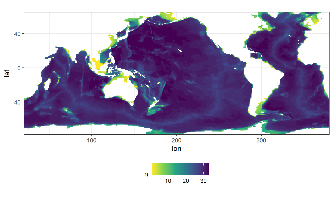
rm(GLODAP_n)2.1.2 WOA18 climatology
WOA18_predictors_n <- WOA18_predictors %>%
  drop_na() %>%
  group_by(lat, lon) %>%
  summarise(n = n()) %>%
  ungroup()

WOA18_predictors_n %>%
  ggplot(aes(lon, lat, fill = n)) +
  geom_raster() +
  scale_fill_viridis_c(direction = -1) +
  coord_quickmap(expand = 0) +
  theme(legend.position = "bottom")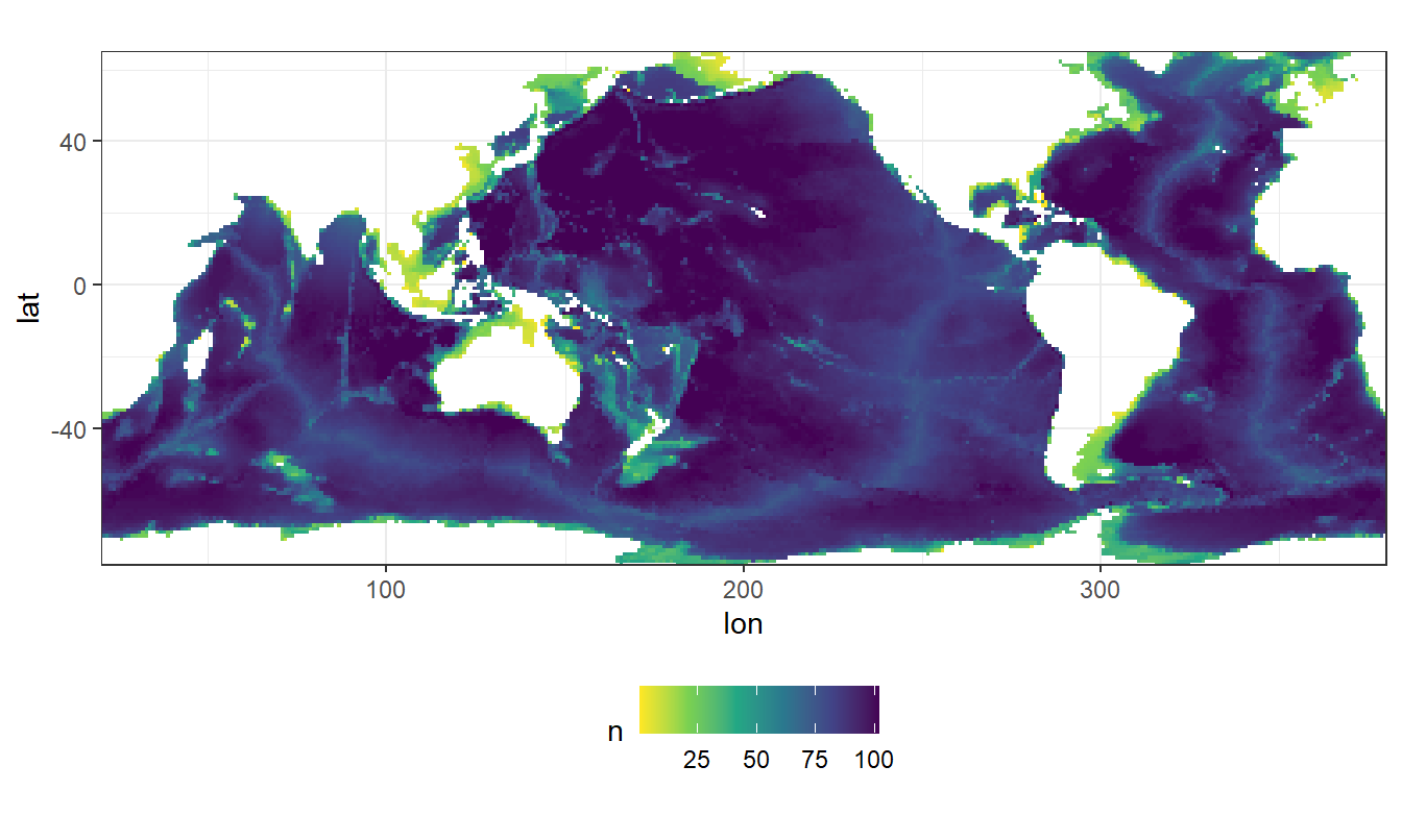
rm(WOA18_predictors_n)2.1.3 Neutral density zonal mean section
WOA18_predictors_zonal <- WOA18_predictors %>%
  group_by(lat, depth, basin) %>%
  summarise(gamma_mean = mean(gamma)) %>%
  ungroup()

WOA18_predictors_zonal_Atl <- WOA18_predictors_zonal %>%
  filter(basin == "Atlantic") %>%
  mutate(gamma_slab = cut(gamma_mean, parameters$slabs_Atl))

WOA18_predictors_zonal_Ind_Pac <- WOA18_predictors_zonal %>%
  filter(basin == "Indo-Pacific") %>%
  mutate(gamma_slab = cut(gamma_mean, parameters$slabs_Ind_Pac))

WOA18_predictors_zonal <- bind_rows(WOA18_predictors_zonal_Atl, WOA18_predictors_zonal_Ind_Pac)

rm(WOA18_predictors_zonal_Atl, WOA18_predictors_zonal_Ind_Pac)

slab_breaks <- c(parameters$slabs_Atl[1:12], Inf)

WOA18_predictors_zonal %>%
  filter(depth <= parameters$inventory_depth) %>%
  ggplot(aes(lat, depth, z = gamma_mean)) +
  geom_contour_filled(breaks = slab_breaks) +
  geom_contour(breaks = slab_breaks,
               col = "white") +
  geom_text_contour(breaks = slab_breaks,
                    col = "white",
                    skip = 1) +
  scale_fill_viridis_d(name = "Gamma",
                       direction = -1) +
  scale_y_reverse() +
  coord_cartesian(expand = 0) +
  guides(fill = guide_colorsteps(barheight = unit(10, "cm"))) +
  facet_grid(basin ~ .)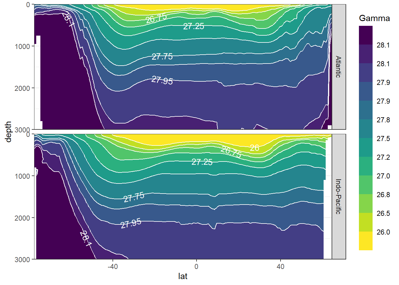
rm(WOA18_predictors_zonal, slab_breaks)2.2 WOA18 + GLODAP
WOA18 and GLODAP predictor climatologies are merged. Only horizontal grid cells with observations from both predictor fields are kept.
GLODAP_depths <- unique(GLODAP_predictors$depth)

predictors <- full_join(GLODAP_predictors, WOA18_predictors)
rm(GLODAP_predictors, WOA18_predictors)

predictors <- predictors %>%
  group_by(lat, lon) %>%
  mutate(n_PO4 = sum(!is.na(PO4)),
         n_sal = sum(!is.na(sal))) %>%
  ungroup()

predictors <- predictors %>%
  filter(n_PO4 > 1,
         n_sal > 1) %>%
  select(-c(n_PO4 , n_sal))
predictors <- predictors %>%
group_by(lat, lon) %>%
arrange(depth) %>%
mutate(tem = approxfun(depth, tem, rule = 2)(depth),
sal = approxfun(depth, sal, rule = 2)(depth),
gamma = approxfun(depth, gamma, rule = 2)(depth)) %>%
ungroup()
predictors <- predictors %>%
filter(depth %in% GLODAP_depths)
rm(GLODAP_depths)2.2.1 Spatial boundaries
Only observations were taken into consideration with:
- minimum sampling depth: 150m
- minimum bottom depth: 500m
- maximum latitude: 65°N
predictors <- predictors %>%
  filter(depth >= parameters$depth_min)

predictors <- predictors %>%
  filter(lat <= parameters$lat_max)

predictors_grid <- predictors %>%
  group_by(lat, lon) %>%
  summarise(bottomdepth = max(depth)) %>%
  ungroup()

predictors <- full_join(predictors, predictors_grid)

predictors <- predictors %>%
  filter(bottomdepth >= parameters$bottomdepth_min) %>%
  select(-bottomdepth)
2.2.2 Control plots
2.2.2.1 Maps
Three maps are generated to control successful merging of data sets.
map_climatology(predictors, "PO4")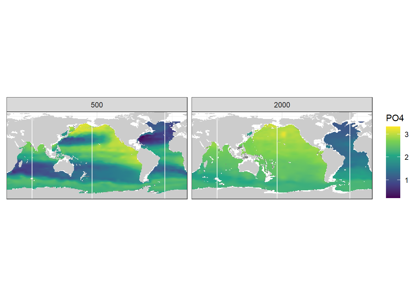
map_climatology(predictors, "tem")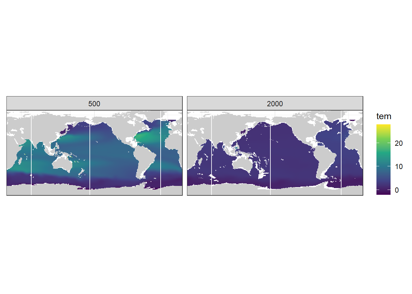
predictors %>%
  ggplot(aes(lon, lat)) +
  geom_bin2d(binwidth = c(1,1)) +
  scale_fill_viridis_c(direction = -1) +
  coord_quickmap(expand = 0) +
  theme(legend.position = "bottom")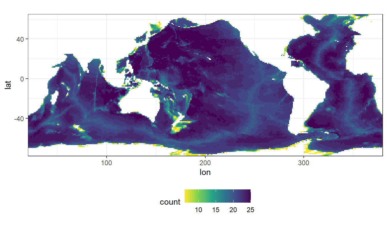
2.2.2.2 Predictor profiles
Likewise, predictor profiles for the North Atlantic are plotted to control successful merging of the data sets.
N_Atl <- predictors %>%
  filter(lat == parameters$lat_Atl_profile,
         lon == parameters$lon_Atl_section)

N_Atl <- N_Atl %>%
  select(-basin) %>%
  pivot_longer(oxygen:gamma, names_to = "parameter", values_to = "value")

N_Atl %>%
  ggplot(aes(value, depth)) +
  geom_path() +
  geom_point() +
  scale_y_reverse() +
  facet_wrap(~parameter,
             scales = "free_x",
             ncol = 2)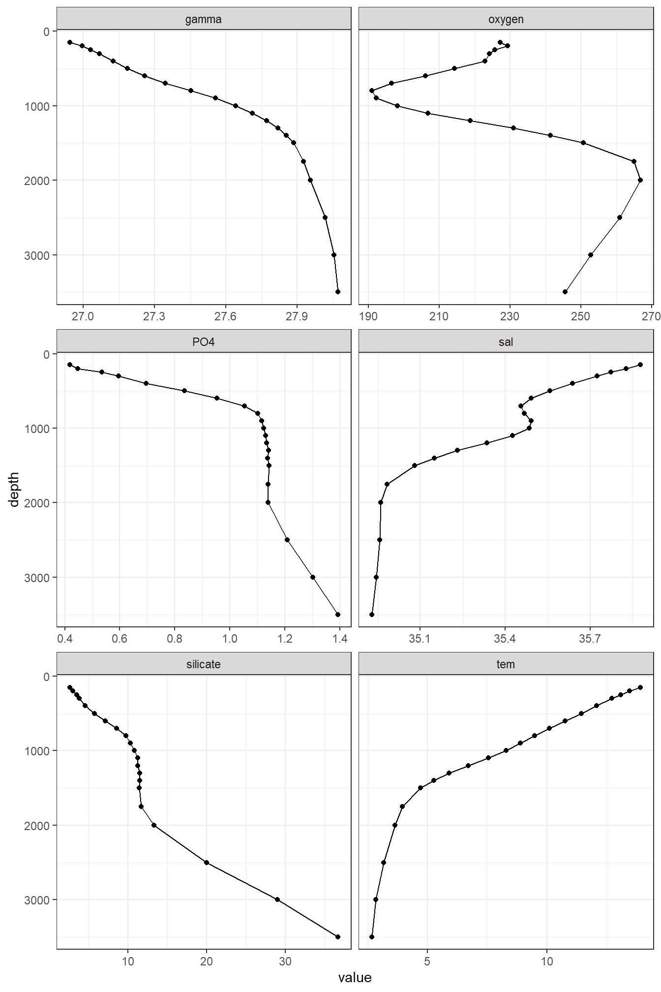
rm(N_Atl)2.2.2.3 Neutral density zonal mean section
predictors_zonal <- predictors %>%
  group_by(lat, depth, basin) %>%
  summarise(gamma_mean = mean(gamma)) %>%
  ungroup()

predictors_zonal_Atl <- predictors_zonal %>%
  filter(basin == "Atlantic") %>%
  mutate(gamma_slab = cut(gamma_mean, parameters$slabs_Atl))

predictors_zonal_Ind_Pac <- predictors_zonal %>%
  filter(basin == "Indo-Pacific") %>%
  mutate(gamma_slab = cut(gamma_mean, parameters$slabs_Ind_Pac))

predictors_zonal <- bind_rows(predictors_zonal_Atl, predictors_zonal_Ind_Pac)

rm(predictors_zonal_Atl, predictors_zonal_Ind_Pac)

slab_breaks <- c(parameters$slabs_Atl[1:12], Inf)

predictors_zonal %>%
  filter(depth <= parameters$inventory_depth) %>%
  ggplot(aes(lat, depth, z = gamma_mean)) +
  geom_contour_filled(breaks = slab_breaks) +
  geom_contour(breaks = slab_breaks,
               col = "white") +
  geom_text_contour(breaks = slab_breaks,
                    col = "white",
                    skip = 1) +
  scale_fill_viridis_d(name = "Gamma",
                       direction = -1) +
  scale_y_reverse() +
  coord_cartesian(expand = 0) +
  guides(fill = guide_colorsteps(barheight = unit(10, "cm"))) +
  facet_grid(basin ~ .)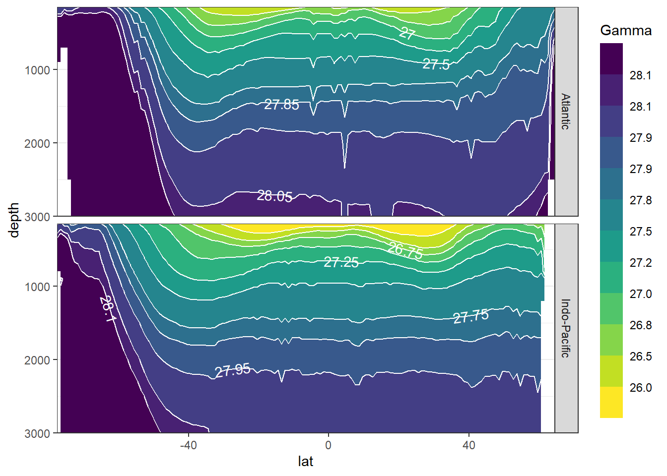
rm(predictors_zonal, slab_breaks)2.3 WOA13 + GLODAP
Currently not used.
predictors <- full_join(GLODAP_predictors, WOA13_gamma)
GLODAP_depths <- unique(GLODAP_predictors$depth)

rm(GLODAP_predictors, WOA13_gamma)

predictors <- predictors %>%
  group_by(lat, lon) %>%
  mutate(n_oxygen = sum(!is.na(oxygen)),
         n_PO4 = sum(!is.na(PO4)),
         n_silicate = sum(!is.na(silicate)),
         n_sal = sum(!is.na(sal)),
         n_tem = sum(!is.na(tem)),
         n_gamma = sum(!is.na(gamma))) %>%
  ungroup()

predictors <- predictors %>%
  filter(n_oxygen > 0,
         n_PO4 > 0,
         n_silicate > 0,
         n_sal > 0,
         n_tem > 0,
         n_gamma > 0) %>%
  select(-c(n_oxygen,
            n_PO4,
            n_silicate,
            n_sal,
            n_tem,
            n_gamma))

predictors <- predictors %>%
  drop_na()
3 Prepare predictor fields
3.1 PO4*
3.1.1 Calculation
Currently, the predictor PO4* is calculated according to Clement and Gruber (2018), ie based on oxygen rather than nitrate.
predictors <- predictors %>%
  rename(phosphate = PO4) %>%
  mutate(phosphate_star = phosphate + (oxygen / 170)  - 1.95)
3.1.2 Maps
map_climatology(predictors, "phosphate_star")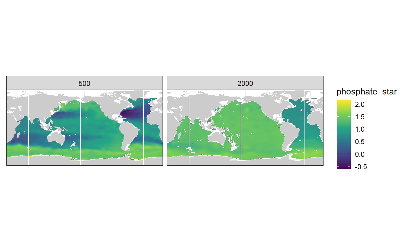
3.1.3 Sections
section_climatology(predictors, "phosphate_star")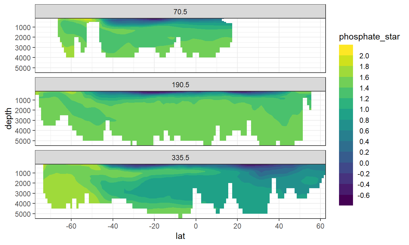
3.2 AOU
3.2.1 Calculation
AOU was calculated as the difference between saturation concentration and observed concentration.
CAVEAT: Algorithms used to calculate oxygen saturation concentration are not yet identical in GLODAP data set (fitting) and predictor climatologies (mapping).
predictors <- predictors %>%
  mutate(oxygen_sat = gas_satconc(S = sal,
                                  t = tem,
                                  P = 1.013253,
                                  species = "O2"),
         aou = oxygen_sat - oxygen) %>%
  select(-oxygen_sat)
3.2.2 Maps
map_climatology(predictors, "aou")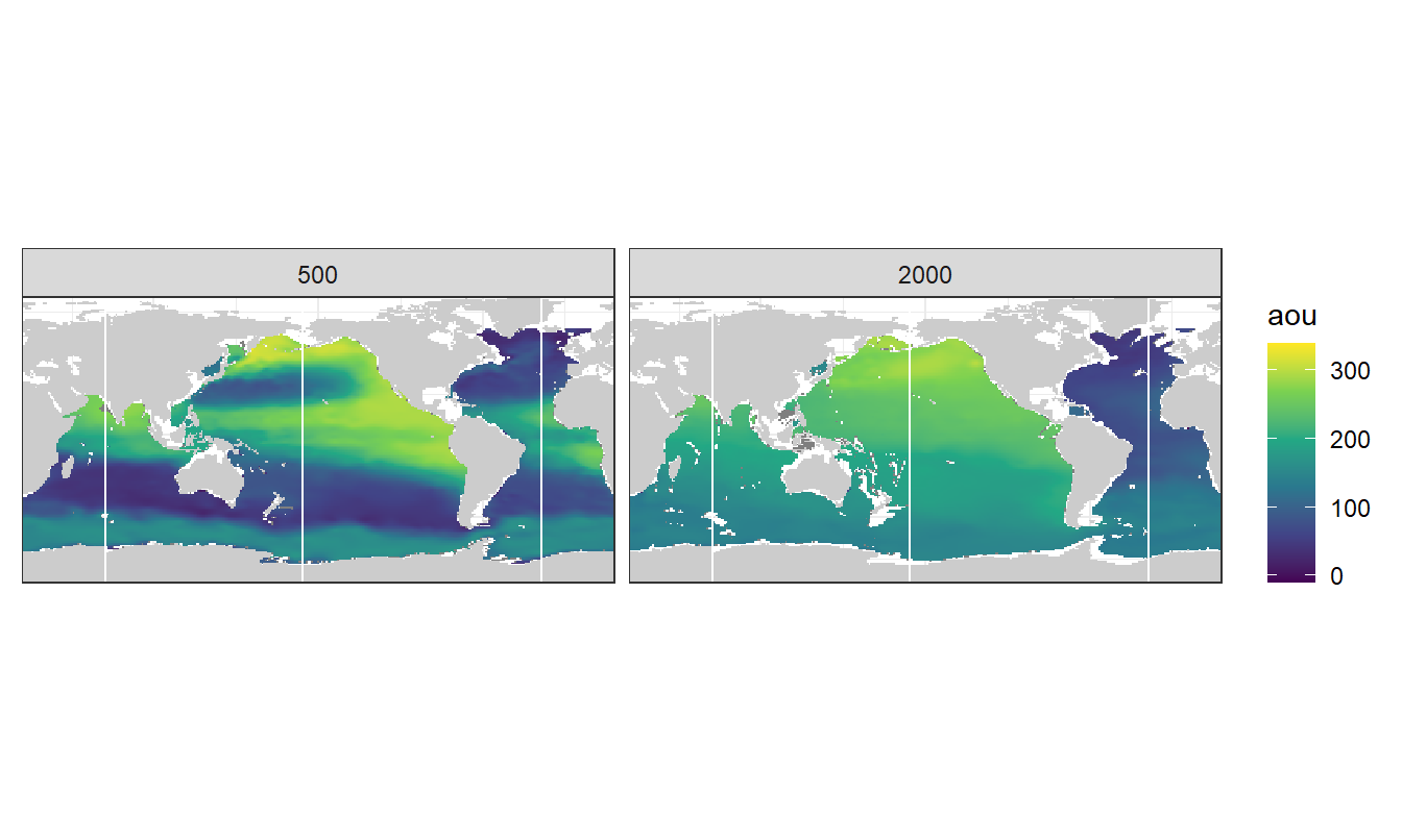
3.2.3 Sections
section_climatology(predictors, "aou")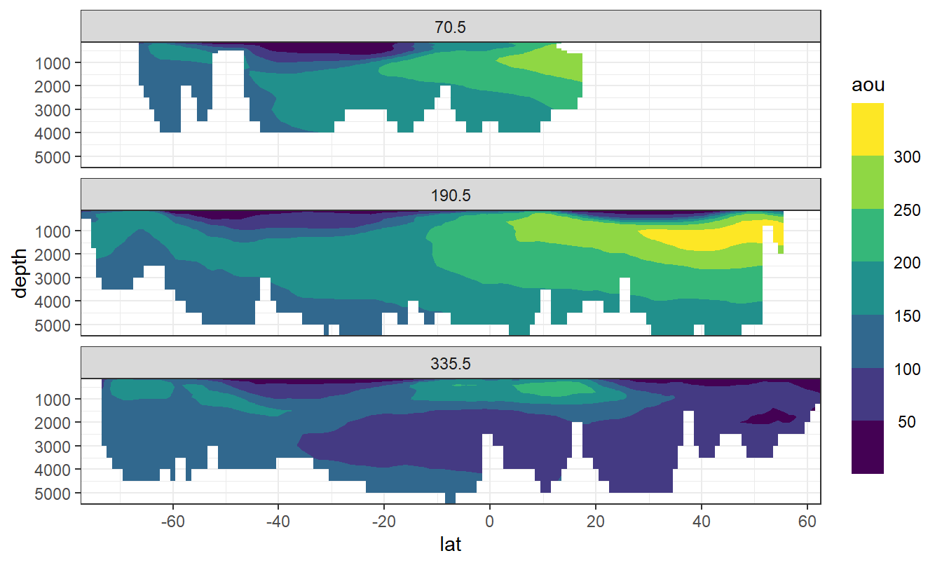
3.3 Isoneutral slabs
The following boundaries for isoneutral slabs were defined:
- Atlantic: -, 26, 26.5, 26.75, 27, 27.25, 27.5, 27.75, 27.85, 27.95, 28.05, 28.1, 28.15, 28.2,
- Indo-Pacific: -, 26, 26.5, 26.75, 27, 27.25, 27.5, 27.75, 27.85, 27.95, 28.05, 28.1,
Continuous neutral density (gamma) values based on WOA13 are grouped into isoneutral slabs.
predictors_Atl <- predictors %>%
  filter(basin == "Atlantic") %>%
  mutate(gamma_slab = cut(gamma, parameters$slabs_Atl))

predictors_Ind_Pac <- predictors %>%
  filter(basin == "Indo-Pacific") %>%
  mutate(gamma_slab = cut(gamma, parameters$slabs_Ind_Pac))

predictors <- bind_rows(predictors_Atl, predictors_Ind_Pac)

rm(predictors_Atl, predictors_Ind_Pac)
4 Prepare model coefficients
all_lm <- all_lm %>%
  select(term, estimate, basin, era, eras, gamma_slab, model)

all_lm <- all_lm %>%
  mutate(estimate = if_else(is.na(estimate), 0, estimate))

all_lm_wide <- all_lm %>%
  pivot_wider(names_from = era, values_from = estimate,
              names_prefix = "coeff_")

all_lm_wide <- all_lm_wide %>%
  mutate(JGOFS_GO = coeff_GO_SHIP - coeff_JGOFS_WOCE,
         GO_new = coeff_new_era - coeff_GO_SHIP) %>%
  select(-c(coeff_JGOFS_WOCE,
            coeff_GO_SHIP,
            coeff_new_era))

all_lm_long <- all_lm_wide %>%
  pivot_longer(JGOFS_GO:GO_new, names_to = "eras_fit", values_to = "delta_coeff")

all_lm_long <- all_lm_long %>%
  filter(eras == eras_fit) %>%
  select(-eras_fit)

all_lm_wide <- all_lm_long %>%
  pivot_wider(values_from = delta_coeff,
              names_from = term,
              names_prefix = "delta_coeff_",
              values_fill = 0)

rm(all_lm_long, all_lm)
4.1 Merge MLRs + climatology
Cant <- full_join(predictors, all_lm_wide)
rm(predictors, all_lm_wide)
5 Map Cant
5.1 Apply MLRs to predictor
Cant <- Cant %>%
  mutate(Cant = `delta_coeff_(Intercept)` +
           delta_coeff_aou * aou +
           delta_coeff_oxygen * oxygen +
           delta_coeff_phosphate * phosphate +
           delta_coeff_phosphate_star * phosphate_star +
           delta_coeff_silicate * silicate +
           delta_coeff_sal * sal +
           delta_coeff_tem * tem)
5.2 Mean Cant fields
Mean and sd are calculated for Cant in each grid cell (XYZ), basin and era combination. Calculations are performed for all Cant values vs positive values only. This averaging step summarizes the information derived from ten best fitting MLRs.
Cant <- Cant %>%
  select(lon, lat, depth, eras, basin, Cant, gamma)

# Cant_model_average <- Cant %>%
#   mutate(Cant_pos = if_else(Cant < 0, 0, Cant)) %>%
#   group_by(lon, lat, depth, eras, basin) %>%
#   summarise(across(c("Cant", "Cant_pos", "gamma"),
#                    list(
#                      mean = ~ mean(.x, na.rm = TRUE),
#                      sd = ~ sd(.x, na.rm = TRUE)
#                    ))) %>%
#   ungroup()

Cant_model_average <- Cant %>%
  mutate(Cant_pos = if_else(Cant < 0, 0, Cant)) %>%
  group_by(lon, lat, depth, eras, basin) %>%
  summarise(Cant_mean = mean(Cant, na.rm = TRUE),
            Cant_sd = sd(Cant, na.rm = TRUE),
            Cant_pos_mean = mean(Cant_pos, na.rm = TRUE),
            Cant_pos_sd = sd(Cant_pos, na.rm = TRUE),
            gamma_mean = mean(gamma, na.rm = TRUE),
            gamma_sd = sd(gamma, na.rm = TRUE)) %>%
  ungroup()

Cant_model_average_Atl <- Cant_model_average %>%
  filter(basin == "Atlantic") %>%
  mutate(gamma_slab = cut(gamma_mean, parameters$slabs_Atl))

Cant_model_average_Ind_Pac <- Cant_model_average %>%
  filter(basin == "Indo-Pacific") %>%
  mutate(gamma_slab = cut(gamma_mean, parameters$slabs_Ind_Pac))

Cant_model_average <- bind_rows(Cant_model_average_Atl, Cant_model_average_Ind_Pac)

rm(Cant_model_average_Atl, Cant_model_average_Ind_Pac)
5.3 Mean Cant sections
For each basin and era combination, the zonal mean Cant is calculated, again for all vs positive only values. Likewise, sd is calculated for the averaging of the mean basin fields.
Cant_model_average_zonal <- Cant_model_average %>%
  group_by(lat, depth, eras, basin) %>%
  summarise(across(
    c(
      "Cant_mean",
      "Cant_pos_mean",
      "Cant_sd",
      "Cant_pos_sd",
      "gamma_mean",
      "gamma_sd"
    ),
    list(mean = ~ mean(.x, na.rm = TRUE),
         sd = ~ sd(.x, na.rm = TRUE))
  )) %>%
  ungroup()


# Cant_model_average_zonal <- Cant_model_average %>%
#   group_by(lat, depth, eras, basin) %>%
#   summarise(Cant_mean_sd = sd(Cant_mean, na.rm = TRUE),
#             Cant_mean = mean(Cant_mean, na.rm = TRUE),
#             Cant_sd_mean = mean(Cant_sd, na.rm = TRUE),
#             Cant_pos_mean_sd = sd(Cant_pos_mean, na.rm = TRUE),
#             Cant_pos_mean = mean(Cant_pos_mean, na.rm = TRUE),
#             Cant_pos_sd_mean = mean(Cant_pos_sd, na.rm = TRUE),
#             gamma_mean = mean(gamma_mean)) %>%
#   ungroup()


Cant_model_average_zonal_Atl <- Cant_model_average_zonal %>%
  filter(basin == "Atlantic") %>%
  mutate(gamma_slab = cut(gamma_mean_mean, parameters$slabs_Atl))

Cant_model_average_zonal_Ind_Pac <- Cant_model_average_zonal %>%
  filter(basin == "Indo-Pacific") %>%
  mutate(gamma_slab = cut(gamma_mean_mean, parameters$slabs_Ind_Pac))

Cant_model_average_zonal <- bind_rows(Cant_model_average_zonal_Atl, Cant_model_average_zonal_Ind_Pac)

rm(Cant_model_average_zonal_Atl, Cant_model_average_zonal_Ind_Pac)
6 Neutral density section
6.1 Mean values
The mean zonal distribution of neutral densities was calculated. CAVEAT: Binning here does not include two highest isoneutral density slabs in the Atlantic, yet.
slab_breaks <- c(parameters$slabs_Atl[1:12],Inf)

Cant_model_average_zonal %>%
  filter(depth <= parameters$inventory_depth) %>%
  ggplot(aes(lat, depth, z = gamma_mean_mean)) +
  geom_contour_filled(breaks = slab_breaks) +
  geom_contour(breaks = slab_breaks,
               col = "white") +
  geom_text_contour(breaks = slab_breaks,
               col = "white",
               skip = 1) +
  scale_fill_viridis_d(name = "Gamma",
                       direction = -1) +
  scale_y_reverse() +
  coord_cartesian(expand = 0) +
  guides(fill = guide_colorsteps(barheight = unit(10, "cm"))) +
  facet_grid(basin~eras)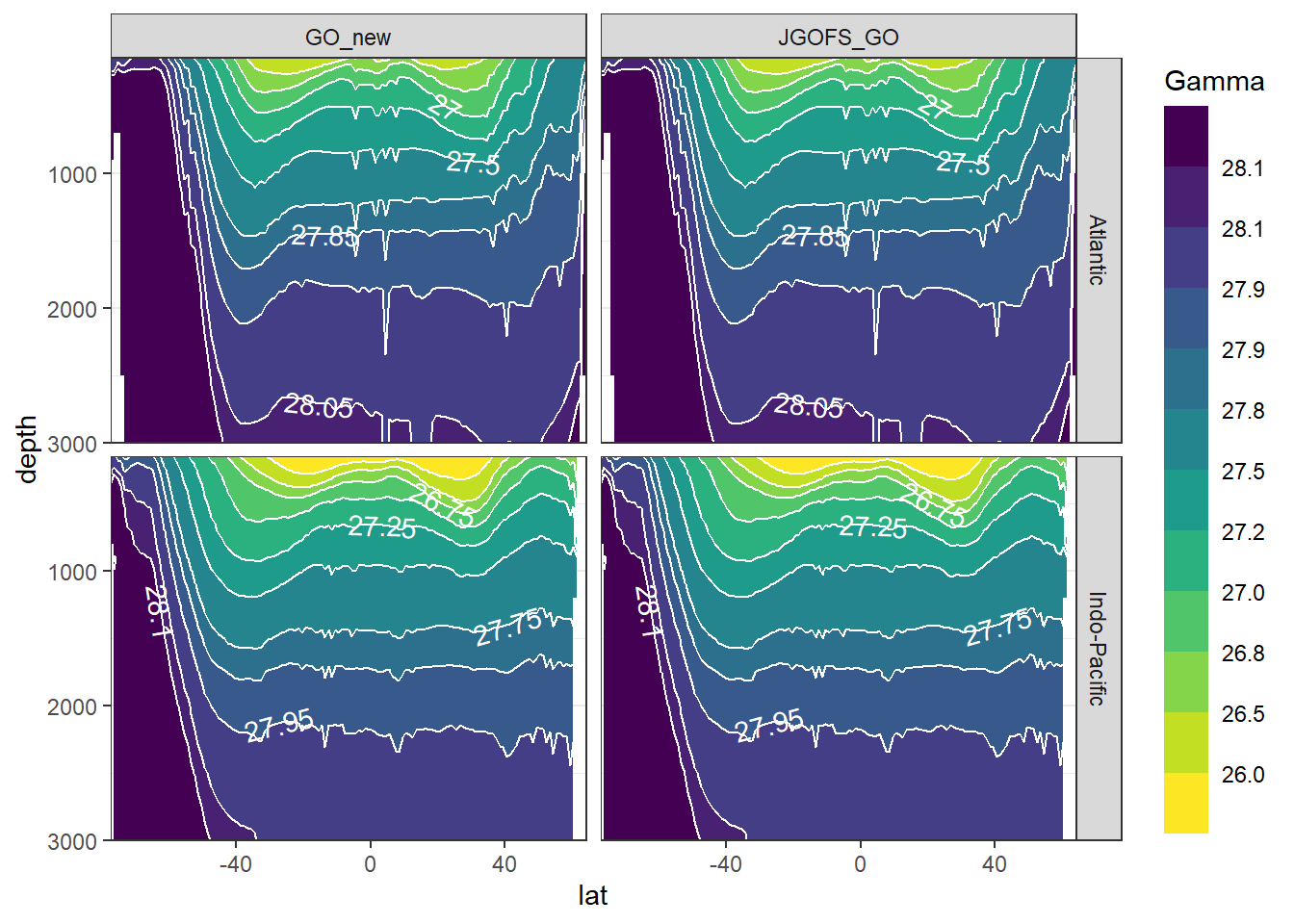
7 Cant sections
7.1 Mean values
Cant_model_average_zonal %>%
  filter(depth <= parameters$inventory_depth) %>%
  ggplot(aes(lat, depth, z = Cant_mean_mean)) +
  geom_contour_fill(breaks = MakeBreaks(5),
                    na.fill = TRUE) +
  scale_fill_divergent(guide = "colorstrip",
                       breaks = MakeBreaks(5),
                       name = "Cant") +
  geom_contour(aes(lat, depth, z = gamma_mean_mean),
               breaks = slab_breaks,
               col = "black") +
  geom_text_contour(
    aes(lat, depth, z = gamma_mean_mean),
    breaks = slab_breaks,
    col = "black",
    skip = 1
  ) +
  scale_y_reverse() +
  coord_cartesian(expand = 0) +
  guides(fill = guide_colorsteps(barheight = unit(10, "cm"))) +
  facet_grid(basin ~ eras)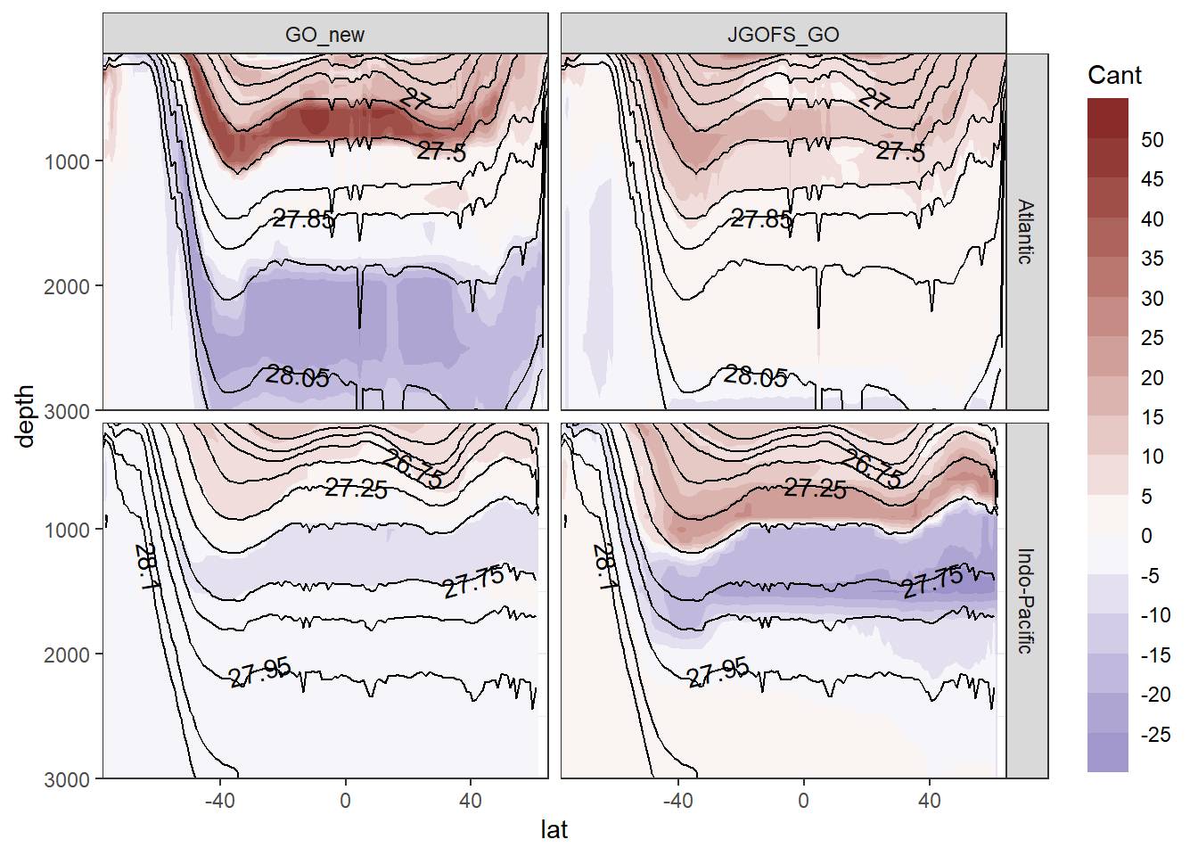
7.2 Mean zonal standard deviation across MLR models
Standard deviation across Cant from all MLR models was calculate for each grid cell (XYZ). The zonal mean of this standard deviation should reflect the uncertainty associated to the predictor selection within each slab and era.
Cant_model_average_zonal %>%
  filter(depth <= parameters$inventory_depth) %>%
  ggplot(aes(lat, depth, z = Cant_sd_mean)) +
  geom_contour_filled() +
  geom_contour(aes(lat, depth, z = gamma_mean_mean),
               breaks = slab_breaks,
               col = "white") +
  geom_text_contour(
    aes(lat, depth, z = gamma_mean_mean),
    breaks = slab_breaks,
    col = "white",
    skip = 1
  ) +
  scale_fill_viridis_d(name = "Cant") +
  scale_y_reverse() +
  coord_cartesian(expand = 0) +
  guides(fill = guide_colorsteps(barheight = unit(10, "cm"))) +
  facet_grid(basin ~ eras)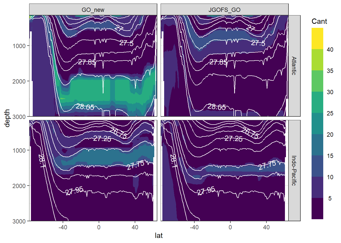
7.3 Zonal standard deviation of mean Cant estimates
Standard deviation of mean Cant values was calculate across all longitudes. This standard deviation should reflect the zonal variability of Cant within the basin and era.
Cant_model_average_zonal %>%
  filter(depth <= parameters$inventory_depth) %>%
  ggplot(aes(lat, depth, z = Cant_mean_sd)) +
  geom_contour_filled() +
  geom_contour(aes(lat, depth, z = gamma_mean_mean),
               breaks = slab_breaks,
               col = "white") +
  geom_text_contour(
    aes(lat, depth, z = gamma_mean_mean),
    breaks = slab_breaks,
    col = "white",
    skip = 1
  ) +
  scale_fill_viridis_d(name = "Cant") +
  scale_y_reverse() +
  coord_cartesian(expand = 0) +
  guides(fill = guide_colorsteps(barheight = unit(10, "cm"))) +
  facet_grid(basin~eras)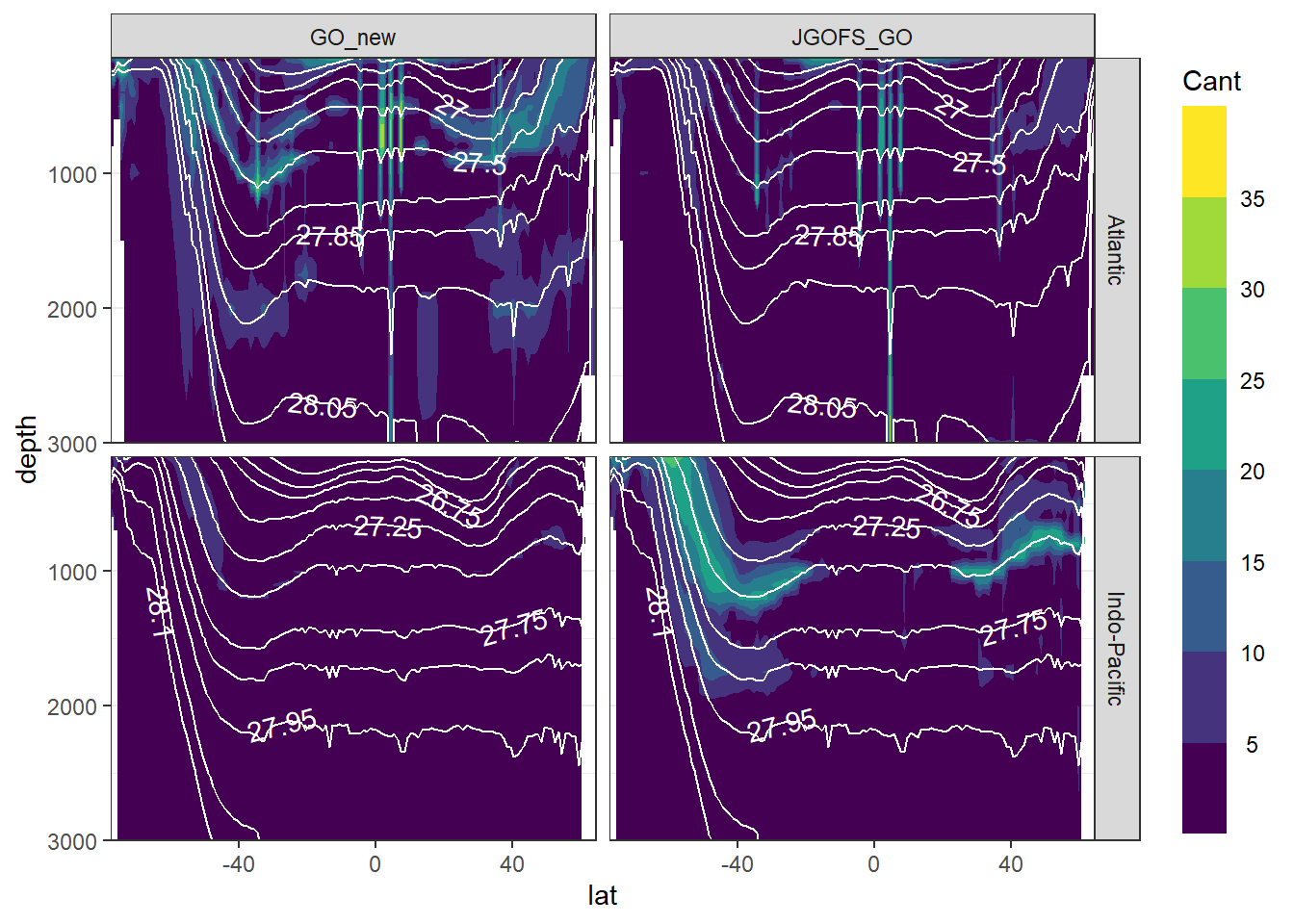
7.4 Mean positive values
Cant_model_average_zonal %>%
  filter(depth <= parameters$inventory_depth) %>%
  ggplot(aes(lat, depth, z = Cant_pos_mean_mean)) +
  geom_contour_filled() +
  geom_contour(aes(lat, depth, z = gamma_mean_mean),
               breaks = slab_breaks,
               col = "white") +
  geom_text_contour(
    aes(lat, depth, z = gamma_mean_mean),
    breaks = slab_breaks,
    col = "white",
    skip = 1
  ) +
  scale_fill_viridis_d(name = "Cant") +
  scale_y_reverse() +
  coord_cartesian(expand = 0) +
  guides(fill = guide_colorsteps(barheight = unit(10, "cm"))) +
  facet_grid(basin~eras)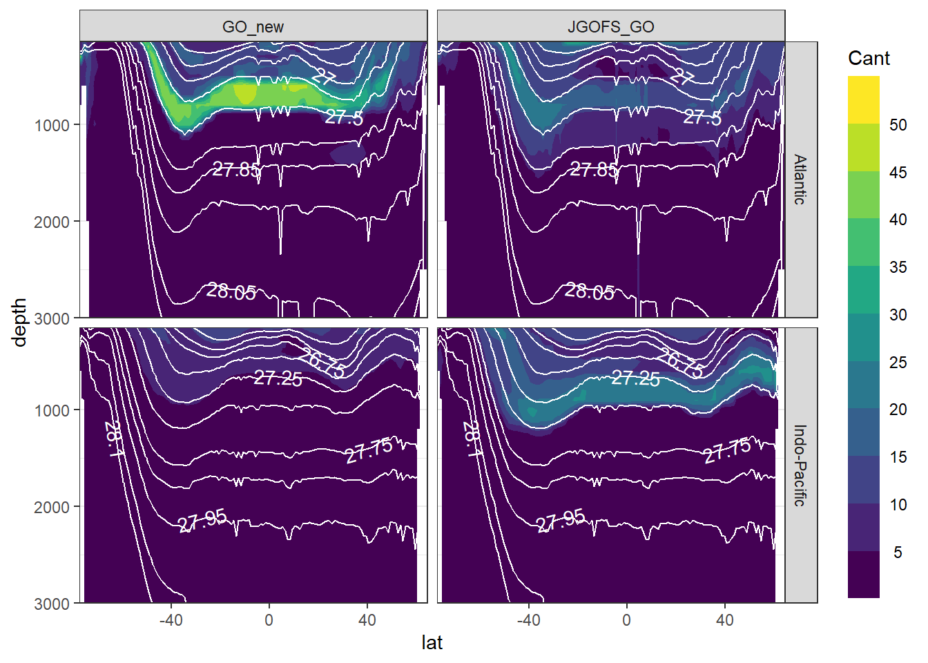
7.5 Sections
7.5.1 JGOFS_GO
section_climatology(Cant_model_average %>% filter(eras == "JGOFS_GO"),
                    "Cant_mean")
7.5.2 GO_new
section_climatology(Cant_model_average %>% filter(eras == "GO_new"),
                    "Cant_mean")
8 Cant maps
8.1 Depth layers
Cant concentration for selected depth levels at which mapping was performed.
Cant_model_average %>%
  filter(depth %in% c(150, 500, 1000, 3000)) %>%
  ggplot(aes(lon, lat, fill = Cant_mean)) +
  geom_raster() +
  scale_fill_divergent(guide = "colorstrip",
                       breaks = MakeBreaks(5),
                       name = "Cant") +
  guides(fill = guide_colorsteps(barheight = unit(10, "cm"))) +
  coord_quickmap(expand = 0) +
  facet_grid(depth~eras)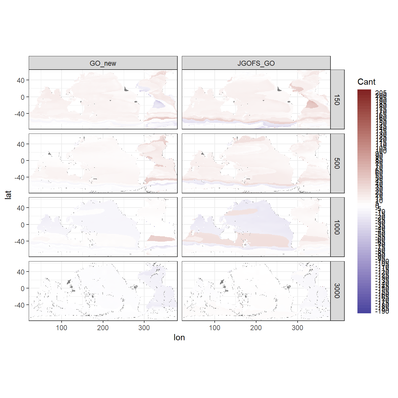
8.2 Inventory calculation
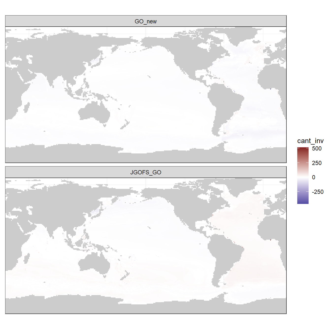
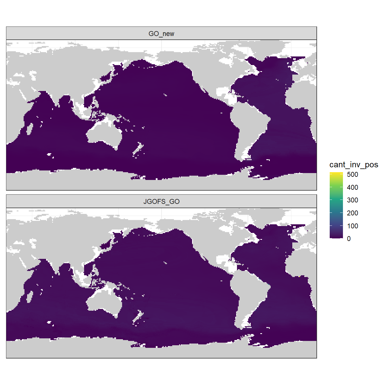
To calculate Cant column inventories, we:
- Multiple layer thickness with Cant concentration to get a layer inventory
- For each horizontal grid cell and era, sum Cant layer inventories from 150 - 3000 m
Step 2 is performed again for all Cant and positive Cant values only
depth_level_volume <- tibble(depth = unique(Cant_model_average$depth))

depth_level_volume <- depth_level_volume %>%
  mutate(
    layer_thickness_above = replace_na((depth - lag(depth)) / 2, 0),
    layer_thickness_below = replace_na((lead(depth) - depth) / 2, 0),
    layer_thickness = layer_thickness_above + layer_thickness_below
  ) %>%
  select(-c(layer_thickness_above,
            layer_thickness_below))

Cant_model_average <-
  full_join(Cant_model_average, depth_level_volume)

Cant_model_average <- Cant_model_average %>%
  mutate(layer_inv = Cant_mean * layer_thickness) %>%
  mutate(layer_inv_pos = if_else(layer_inv < 0, 0, layer_inv)) %>%
  select(-layer_thickness)

Cant_inv <- Cant_model_average %>%
  filter(depth <= parameters$inventory_depth) %>%
  group_by(lon, lat, basin, eras) %>%
  summarise(
    cant_inv_pos = sum(layer_inv_pos, na.rm = TRUE) / 1000,
    cant_inv     = sum(layer_inv, na.rm = TRUE) / 1000
  ) %>%
  ungroup()
8.3 Inventories
8.3.1 All Cant estimates
library(scales)

Cant_inv %>%
  ggplot() +
    geom_raster(data = landmask %>% filter(region == "land"),
                aes(lon, lat), fill = "grey80") +
    geom_raster(aes(lon, lat, fill = cant_inv)) +
    coord_quickmap(expand = 0) +
    scale_fill_gradient2(high = muted("red"),
                         mid = "white",
                         low = muted("blue"),
                         midpoint = 0,
                         space = "Lab",
                         na.value = "green") +
  facet_wrap(~eras, ncol = 1) +
    theme(
      axis.title = element_blank(),
      axis.text = element_blank(),
      axis.ticks = element_blank()
    )
8.3.2 Positive Cant estimates
Cant_inv %>%
  ggplot() +
    geom_raster(data = landmask %>% filter(region == "land"),
                aes(lon, lat), fill = "grey80") +
    geom_raster(aes(lon, lat, fill = cant_inv_pos)) +
    coord_quickmap(expand = 0) +
    scale_fill_viridis_c() +
  facet_wrap(~eras, ncol = 1) +
    theme(
      axis.title = element_blank(),
      axis.text = element_blank(),
      axis.ticks = element_blank()
    )
9 Write csv
Cant_model_average %>%
    write_csv(here::here("data/mapping/_summarized_files",
                         "Cant_2020.csv"))

Cant_inv %>%
    write_csv(here::here("data/mapping/_summarized_files",
                         "Cant_inv_2020.csv"))
10 Open tasks
- Check PO4* calculation
- Harmonize AOU calculation in fitting and mapping
- Plot Cant sections for individual MLR models
11 Open questions
sessionInfo()R version 4.0.2 (2020-06-22)
Platform: x86_64-w64-mingw32/x64 (64-bit)
Running under: Windows 10 x64 (build 18363)
Matrix products: default
locale:
[1] LC_COLLATE=English_Germany.1252 LC_CTYPE=English_Germany.1252
[3] LC_MONETARY=English_Germany.1252 LC_NUMERIC=C
[5] LC_TIME=English_Germany.1252
attached base packages:
[1] stats graphics grDevices utils datasets methods base
other attached packages:
[1] scales_1.1.1 reticulate_1.16 metR_0.7.0 marelac_2.1.10
[5] shape_1.4.4 oce_1.2-0 gsw_1.0-5 testthat_2.3.2
[9] lubridate_1.7.9 forcats_0.5.0 stringr_1.4.0 dplyr_1.0.0
[13] purrr_0.3.4 readr_1.3.1 tidyr_1.1.0 tibble_3.0.3
[17] ggplot2_3.3.2 tidyverse_1.3.0 workflowr_1.6.2
loaded via a namespace (and not attached):
[1] httr_1.4.2 jsonlite_1.7.0 viridisLite_0.3.0 here_0.1
[5] modelr_0.1.8 assertthat_0.2.1 sp_1.4-2 blob_1.2.1
[9] cellranger_1.1.0 yaml_2.2.1 pillar_1.4.6 backports_1.1.8
[13] lattice_0.20-41 glue_1.4.1 digest_0.6.25 promises_1.1.1
[17] checkmate_2.0.0 rvest_0.3.6 colorspace_1.4-1 plyr_1.8.6
[21] htmltools_0.5.0 httpuv_1.5.4 Matrix_1.2-18 pkgconfig_2.0.3
[25] broom_0.7.0 seacarb_3.2.13 haven_2.3.1 whisker_0.4
[29] later_1.1.0.1 git2r_0.27.1 generics_0.0.2 farver_2.0.3
[33] ellipsis_0.3.1 withr_2.2.0 cli_2.0.2 magrittr_1.5
[37] crayon_1.3.4 readxl_1.3.1 memoise_1.1.0 evaluate_0.14
[41] fs_1.4.2 fansi_0.4.1 xml2_1.3.2 tools_4.0.2
[45] data.table_1.13.0 hms_0.5.3 lifecycle_0.2.0 munsell_0.5.0
[49] reprex_0.3.0 isoband_0.2.2 compiler_4.0.2 rlang_0.4.7
[53] grid_4.0.2 rstudioapi_0.11 labeling_0.3 rmarkdown_2.3
[57] gtable_0.3.0 DBI_1.1.0 R6_2.4.1 knitr_1.29
[61] rprojroot_1.3-2 stringi_1.4.6 Rcpp_1.0.5 vctrs_0.3.2
[65] dbplyr_1.4.4 tidyselect_1.1.0 xfun_0.16