Last updated: 2026-03-17

Checks: 6 1

Knit directory: HonorsThesis/

This reproducible R Markdown analysis was created with workflowr (version 1.7.2). The Checks tab describes the reproducibility checks that were applied when the results were created. The Past versions tab lists the development history.


The R Markdown file has unstaged changes. To know which version of the R Markdown file created these results, you’ll want to first commit it to the Git repo. If you’re still working on the analysis, you can ignore this warning. When you’re finished, you can run wflow_publish to commit the R Markdown file and build the HTML.

Great job! The global environment was empty. Objects defined in the global environment can affect the analysis in your R Markdown file in unknown ways. For reproduciblity it’s best to always run the code in an empty environment.

The command set.seed(20260127) was run prior to running the code in the R Markdown file. Setting a seed ensures that any results that rely on randomness, e.g. subsampling or permutations, are reproducible.

Great job! Recording the operating system, R version, and package versions is critical for reproducibility.

Nice! There were no cached chunks for this analysis, so you can be confident that you successfully produced the results during this run.

Great job! Using relative paths to the files within your workflowr project makes it easier to run your code on other machines.

Great! You are using Git for version control. Tracking code development and connecting the code version to the results is critical for reproducibility.

The results in this page were generated with repository version 3216d85. See the Past versions tab to see a history of the changes made to the R Markdown and HTML files.

Note that you need to be careful to ensure that all relevant files for the analysis have been committed to Git prior to generating the results (you can use wflow_publish or wflow_git_commit). workflowr only checks the R Markdown file, but you know if there are other scripts or data files that it depends on. Below is the status of the Git repository when the results were generated:


Ignored files:
    Ignored:    .DS_Store
    Ignored:    .claude/
    Ignored:    renv/library/
    Ignored:    renv/staging/

Unstaged changes:
    Modified:   Data/period_dictionary.csv
    Modified:   analysis/cups_and_skulls_analysis.Rmd

Note that any generated files, e.g. HTML, png, CSS, etc., are not included in this status report because it is ok for generated content to have uncommitted changes.


These are the previous versions of the repository in which changes were made to the R Markdown (analysis/cups_and_skulls_analysis.Rmd) and HTML (docs/cups_and_skulls_analysis.html) files. If you’ve configured a remote Git repository (see ?wflow_git_remote), click on the hyperlinks in the table below to view the files as they were in that past version.

File Version Author Date Message
Rmd 3216d85 tinalasisi 2026-03-10 fixed the period name overlap
html 3216d85 tinalasisi 2026-03-10 fixed the period name overlap
Rmd 7857fa6 tinalasisi 2026-03-10 Added hair pin analyses + messed around with figure to make them prettier
html 7857fa6 tinalasisi 2026-03-10 Added hair pin analyses + messed around with figure to make them prettier
html 352636f tinalasisi 2026-02-17 Build site.
Rmd 27b3161 tinalasisi 2026-02-17 Add comprehensive guiding comments for student customization
html 01b0d46 tinalasisi 2026-02-17 Build site.
Rmd 2410c8d tinalasisi 2026-02-17 Add dictionary loading template and switch to grouped bar plots
html 8d3e1c7 tinalasisi 2026-02-17 Build site.
Rmd d689566 tinalasisi 2026-02-17 Add color customization and region-based faceted plots
html 2f9f6dc tinalasisi 2026-02-17 Build site.
Rmd c592bd3 tinalasisi 2026-02-17 Add data dictionary worksheet and chamber space analysis

Introduction

This document presents the quantitative analyses underlying the thesis. The dataset comprises funerary contexts from Laconia and Messenia spanning the Middle Helladic through Late Helladic periods (approximately 2000–1070 BCE). Each record corresponds to a single tomb or grave feature and includes information on tomb type, chronological attribution, burial practice, and the presence of drinking vessels, skeletal remains, and hair pins.

The analyses address four main questions: (1) how tomb types and burial practices are distributed across the two regions; (2) whether drinking vessels and skeletal remains co-occur in patterned ways; (3) whether hair pins cluster with particular burial practices, vessel assemblages, or tomb sizes; and (4) how these variables change over the course of the Bronze Age. All code is folded by default and can be expanded for inspection.

Load Libraries

knitr::opts_chunk$set(warning = FALSE, message = FALSE)
library(readr)
library(dplyr)
library(ggplot2)
library(tidyr)
library(stringr)
library(janitor)
library(knitr)
library(kableExtra)
library(broom)
library(ggrepel)

Visualization Settings

# Set your color palette here
colors <- list(
  laconia = "#1B9E77",      # Laconia color (default: teal/green)
  messenia = "#D95F02",     # Messenia color (default: orange)
  drinking_vessel = "#7570B3",  # Drinking vessels (default: purple)
  skulls = "#E7298A",        # Skulls (default: pink)
  pin = "#E6AB02",            # Hair pins (default: gold/amber)
  background = "#FFFFCC"     # Background/neutral (default: light yellow)
)

# These colors will be used throughout all plots
# Change the hex codes to your preferred colors

# Set global ggplot theme with larger text
theme_set(theme_minimal(base_size = 16))
theme_update(
  plot.title = element_text(size = 18, face = "bold"),
  plot.subtitle = element_text(size = 14),
  axis.title = element_text(size = 14),
  axis.text = element_text(size = 12),
  legend.text = element_text(size = 12),
  legend.title = element_text(size = 13),
  strip.text = element_text(size = 13)
)

Data Source

# Load the CSV data
data_path <- here::here("data", "laconia_messinia_cups_skulls_pins.csv")
cups_skulls <- read_csv(data_path)

# Display dimensions
cat("Dataset dimensions:", nrow(cups_skulls), "graves ×", ncol(cups_skulls), "columns\n")
Dataset dimensions: 296 graves × 15 columns
# Show column names
glimpse(cups_skulls)
Rows: 296
Columns: 15
$ `Grave ID`                  <chr> "vapheio_tholos", "arkynes_tholos_A", "ark…
$ site                        <chr> "Vapheio", "Arkynes", "Arkynes", "Arkynes"…
$ type                        <chr> "tholos", "tholos", "tholos", "tholos", "t…
$ period                      <chr> "LHIIA-LHIIIA1", "LHIIIA- LHIIIB", "LHIII"…
$ secondary                   <chr> "absent", "absent", "absent", "present", "…
$ primary                     <chr> "absent", "absent", "present", "absent", "…
$ dimensions                  <chr> "83.28m^2. dromos: L 29.8m x w3.18-3.45, s…
$ orientation                 <chr> "NE-SW", "SE-NW", NA, NA, "E-W", "N-S", "W…
$ `drinking vessel`           <chr> "yes", "no", "no", "no", "no", "no", "no",…
$ remains                     <chr> "yes", "yes", "yes", "yes", "yes", "no", "…
$ `drinking vessel number`    <dbl> 6, NA, NA, NA, NA, NA, NA, 4, NA, NA, 5, N…
$ `skulls number`             <dbl> NA, NA, NA, NA, NA, NA, NA, NA, NA, NA, NA…
$ `area of chamber estimated` <dbl> 84.130, 17.350, NA, 28.274, 7.793, NA, 18.…
$ region                      <chr> "laconia", "laconia", "laconia", "laconia"…
$ `hair pin`                  <chr> "yes", "no", "no", "yes", "no", "no", "no"…

Data Preparation

Variable Coding

Raw text fields were recoded into analysis-ready variables. Drinking vessel presence, skeletal remains, and hair pin presence were each recorded as binary yes/no fields in the spreadsheet and converted to logical values (TRUE/FALSE); entries that could not be classified were retained as NA and excluded from relevant calculations. Primary and secondary burial were coded from “present”/“absent” fields in the same way.

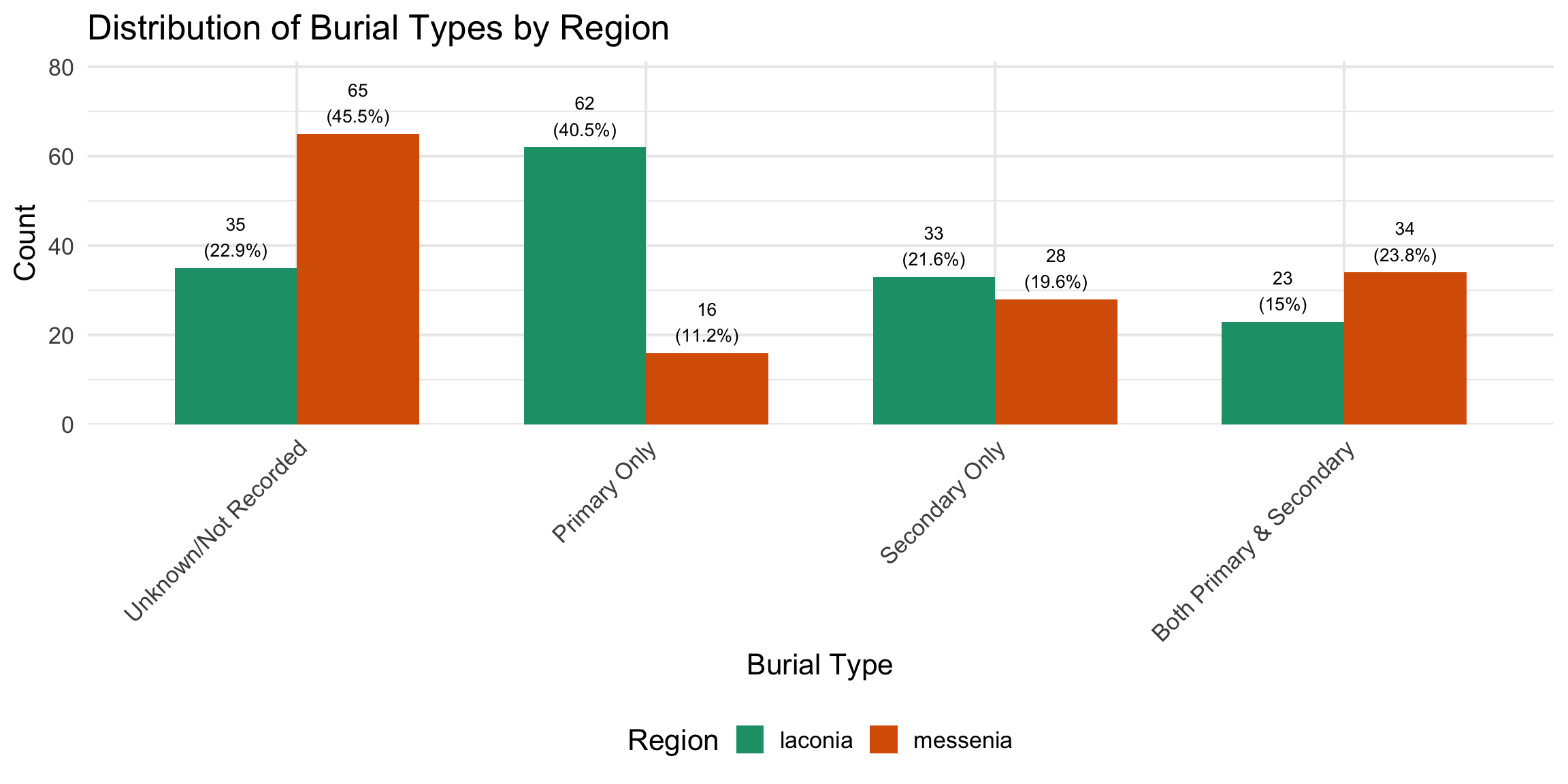
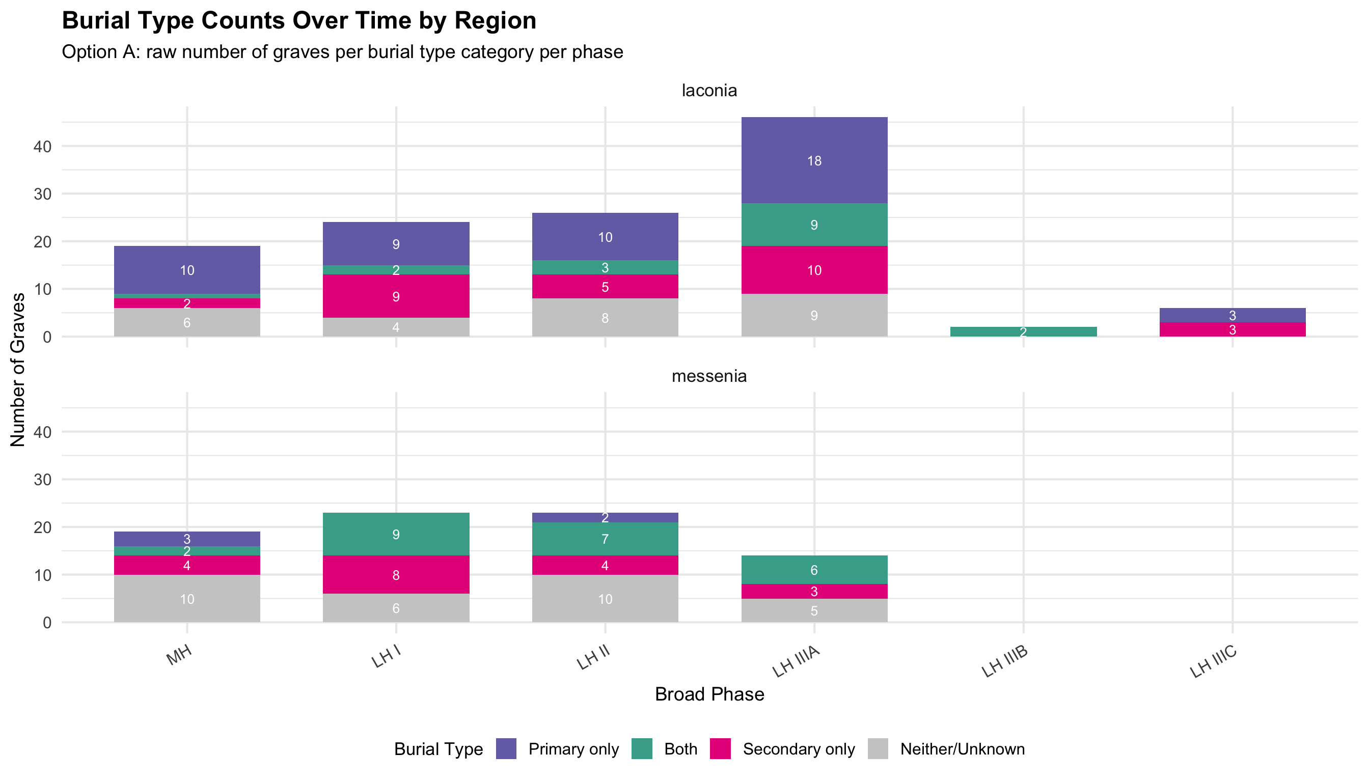
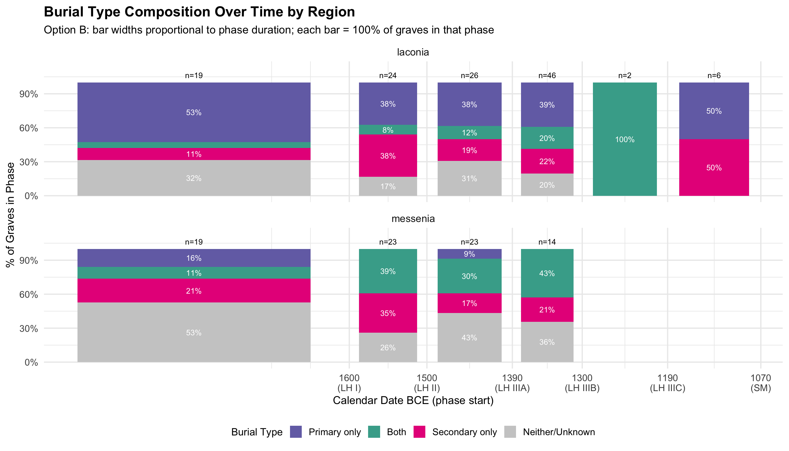
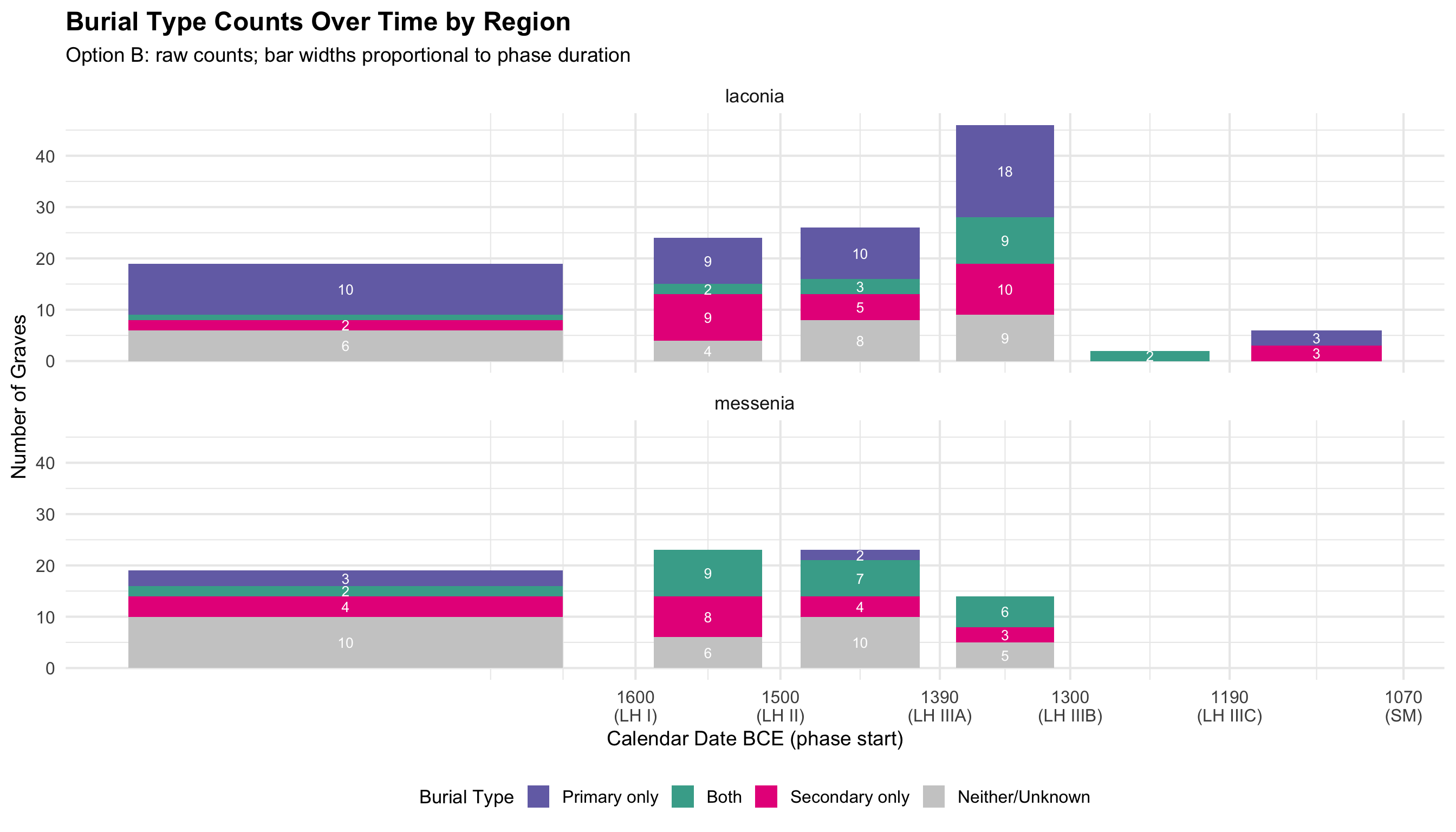
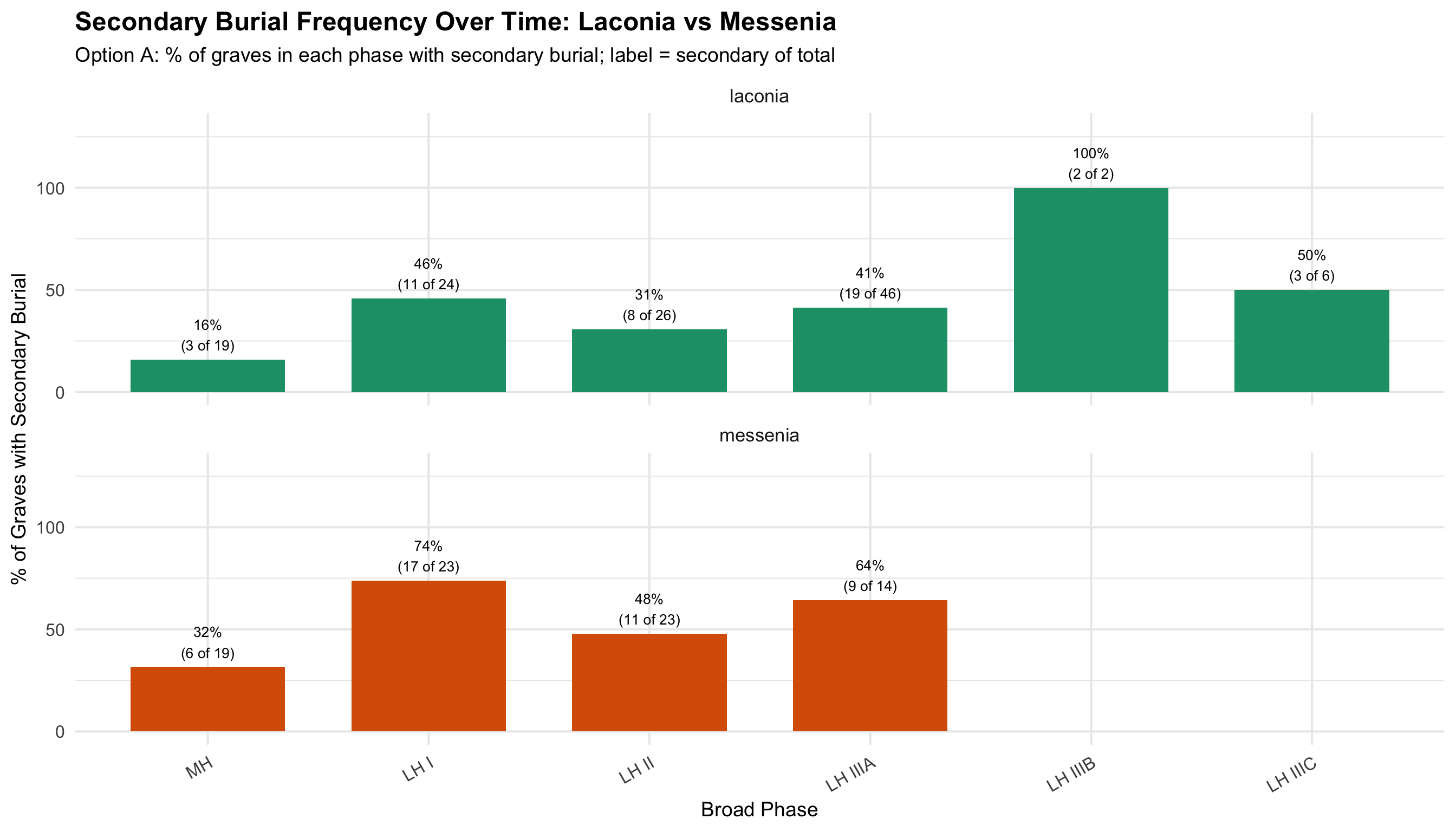
Burial contexts were then classified into four mutually exclusive categories based on the combination of primary and secondary burial evidence: Primary Only, Secondary Only, Both Primary and Secondary, and Unknown/Not Recorded. Tomb 
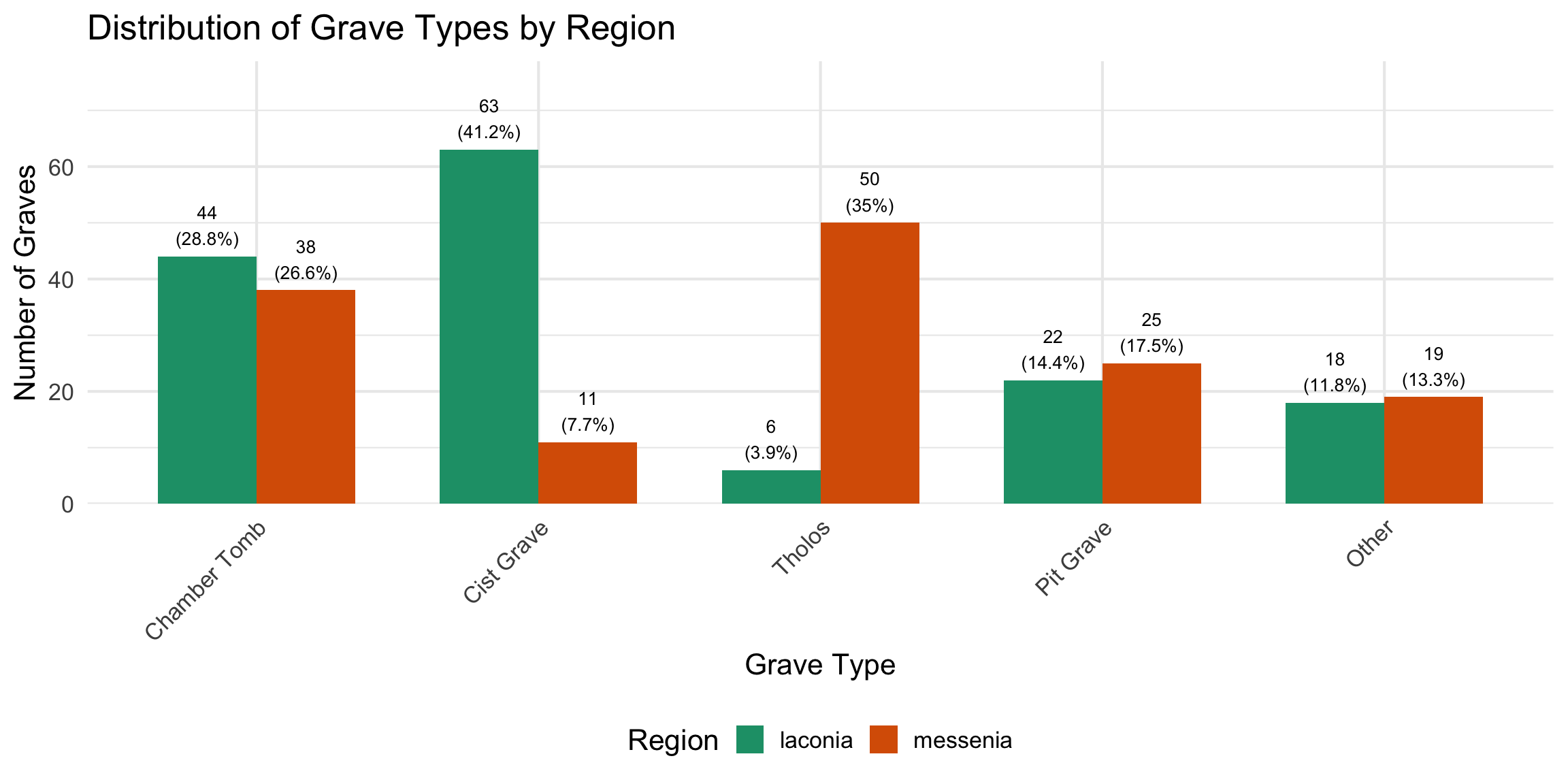
types were simplified from their original descriptive labels into five structural categories — Tholos, Chamber Tomb, Cist Grave, Pit Grave, and Dromos Only — to allow comparison across sites where nomenclature varies.

cups_skulls_clean <- cups_skulls %>%
  # Clean column names
  janitor::clean_names() %>%

  # Trim whitespace from character columns
  mutate(across(where(is.character), str_trim)) %>%

  # Standardize yes/no values in drinking vessel column
  mutate(
    has_drinking_vessel = case_when(
      tolower(drinking_vessel) == "yes" ~ TRUE,
      tolower(drinking_vessel) == "no" ~ FALSE,
      TRUE ~ NA
    ),
    has_remains = case_when(
      tolower(remains) == "yes" ~ TRUE,
      tolower(remains) == "no" ~ FALSE,
      TRUE ~ NA
    ),
    primary_burial = case_when(
      tolower(primary) == "present" ~ TRUE,
      tolower(primary) == "absent" ~ FALSE,
      TRUE ~ NA
    ),
    secondary_burial = case_when(
      tolower(secondary) == "present" ~ TRUE,
      tolower(secondary) == "absent" ~ FALSE,
      TRUE ~ NA
    ),
    has_pin = case_when(
      tolower(hair_pin) == "yes" ~ TRUE,
      tolower(hair_pin) == "no" ~ FALSE,
      TRUE ~ NA
    )
  ) %>%

  # Create burial category
  mutate(
    burial_category = case_when(
      primary_burial & secondary_burial ~ "Both Primary & Secondary",
      primary_burial & !secondary_burial ~ "Primary Only",
      !primary_burial & secondary_burial ~ "Secondary Only",
      TRUE ~ "Unknown/Not Recorded"
    )
  ) %>%

  # Simplify grave type
  # ** YOU CAN CUSTOMIZE THIS SECTION **
  # If you want different groupings, edit the patterns here
  # Current grouping is based on archaeological complexity
  mutate(
    grave_type_simple = case_when(
      str_detect(tolower(type), "tholos") ~ "Tholos",
      str_detect(tolower(type), "chamber") ~ "Chamber Tomb",
      str_detect(tolower(type), "cist") ~ "Cist Grave",
      str_detect(tolower(type), "pit") ~ "Pit Grave",
      str_detect(tolower(type), "dromos") ~ "Dromos Only",
      TRUE ~ "Other"
    )
  )

# Show cleaned data structure
glimpse(cups_skulls_clean)
Rows: 296
Columns: 22
$ grave_id                  <chr> "vapheio_tholos", "arkynes_tholos_A", "arkyn…
$ site                      <chr> "Vapheio", "Arkynes", "Arkynes", "Arkynes", …
$ type                      <chr> "tholos", "tholos", "tholos", "tholos", "tho…
$ period                    <chr> "LHIIA-LHIIIA1", "LHIIIA- LHIIIB", "LHIII", …
$ secondary                 <chr> "absent", "absent", "absent", "present", "pr…
$ primary                   <chr> "absent", "absent", "present", "absent", "pr…
$ dimensions                <chr> "83.28m^2. dromos: L 29.8m x w3.18-3.45, sto…
$ orientation               <chr> "NE-SW", "SE-NW", NA, NA, "E-W", "N-S", "W-E…
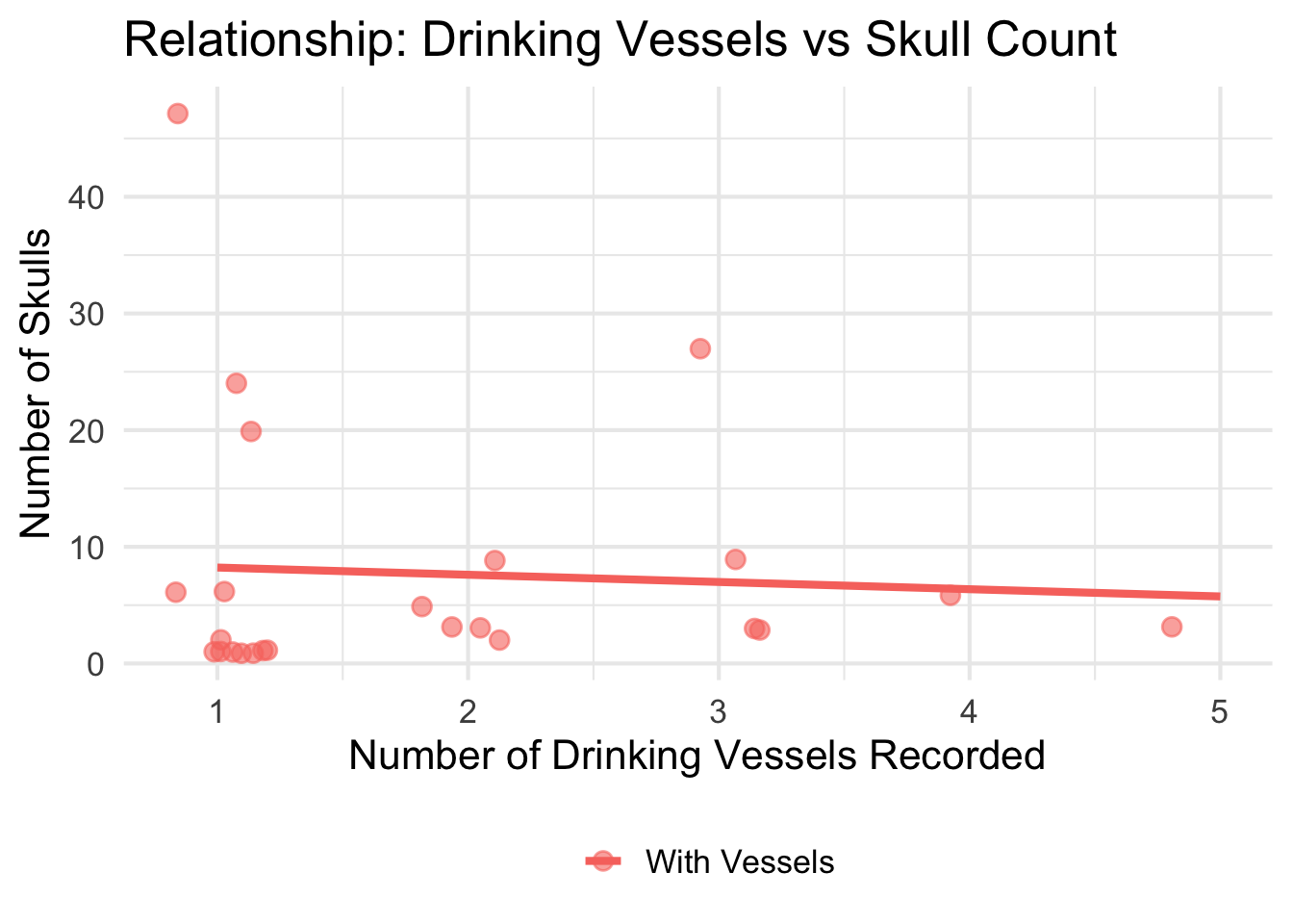
$ drinking_vessel           <chr> "yes", "no", "no", "no", "no", "no", "no", "…
$ remains                   <chr> "yes", "yes", "yes", "yes", "yes", "no", "no…
$ drinking_vessel_number    <dbl> 6, NA, NA, NA, NA, NA, NA, 4, NA, NA, 5, NA,…
$ skulls_number             <dbl> NA, NA, NA, NA, NA, NA, NA, NA, NA, NA, NA, …
$ area_of_chamber_estimated <dbl> 84.130, 17.350, NA, 28.274, 7.793, NA, 18.32…
$ region                    <chr> "laconia", "laconia", "laconia", "laconia", …
$ hair_pin                  <chr> "yes", "no", "no", "yes", "no", "no", "no", …
$ has_drinking_vessel       <lgl> TRUE, FALSE, FALSE, FALSE, FALSE, FALSE, FAL…
$ has_remains               <lgl> TRUE, TRUE, TRUE, TRUE, TRUE, FALSE, FALSE, …
$ primary_burial            <lgl> FALSE, FALSE, TRUE, FALSE, TRUE, FALSE, FALS…
$ secondary_burial          <lgl> FALSE, FALSE, FALSE, TRUE, TRUE, FALSE, FALS…
$ has_pin                   <lgl> TRUE, FALSE, FALSE, TRUE, FALSE, FALSE, FALS…
$ burial_category           <chr> "Unknown/Not Recorded", "Unknown/Not Recorde…
$ grave_type_simple         <chr> "Tholos", "Tholos", "Tholos", "Tholos", "Tho…

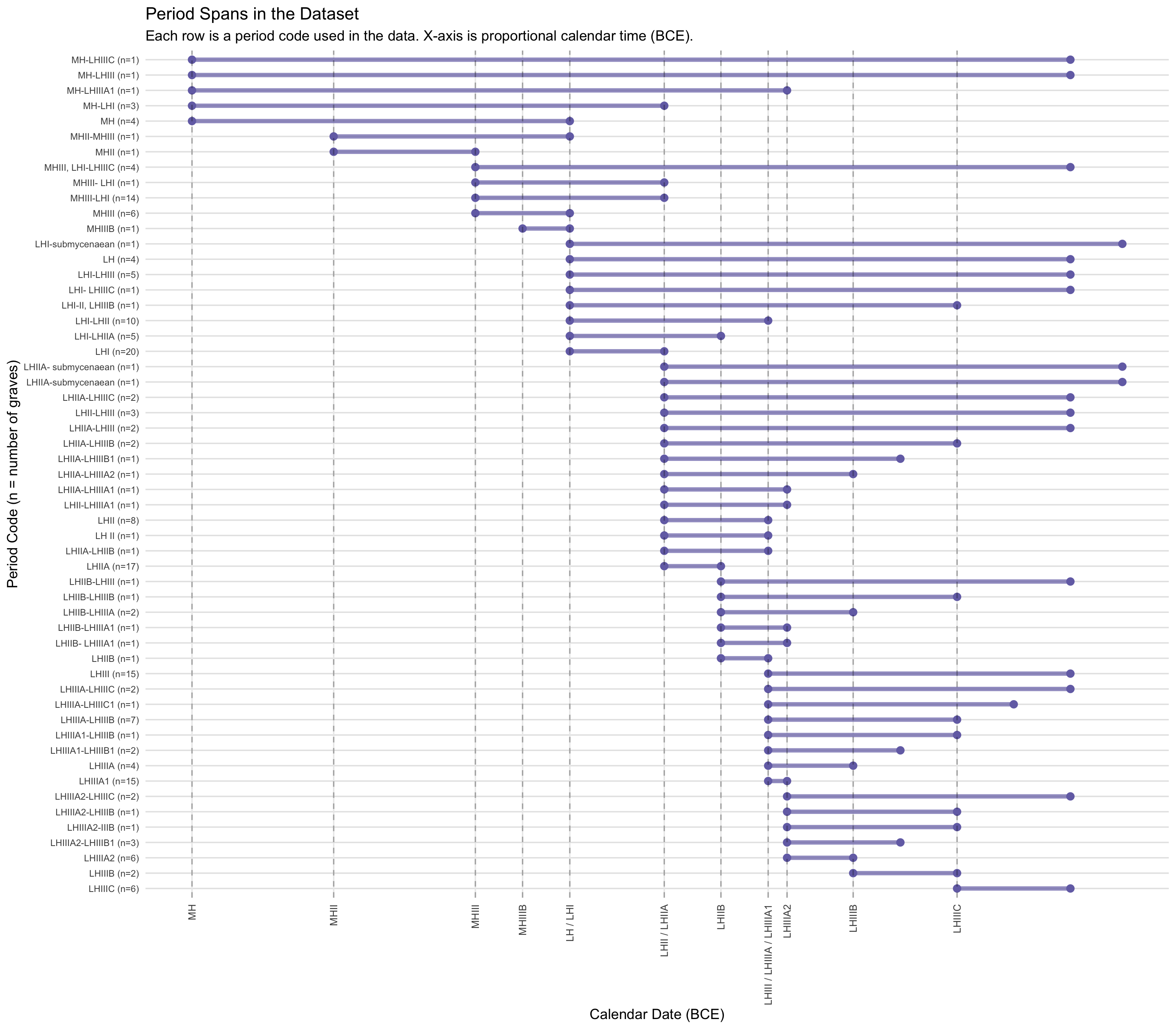
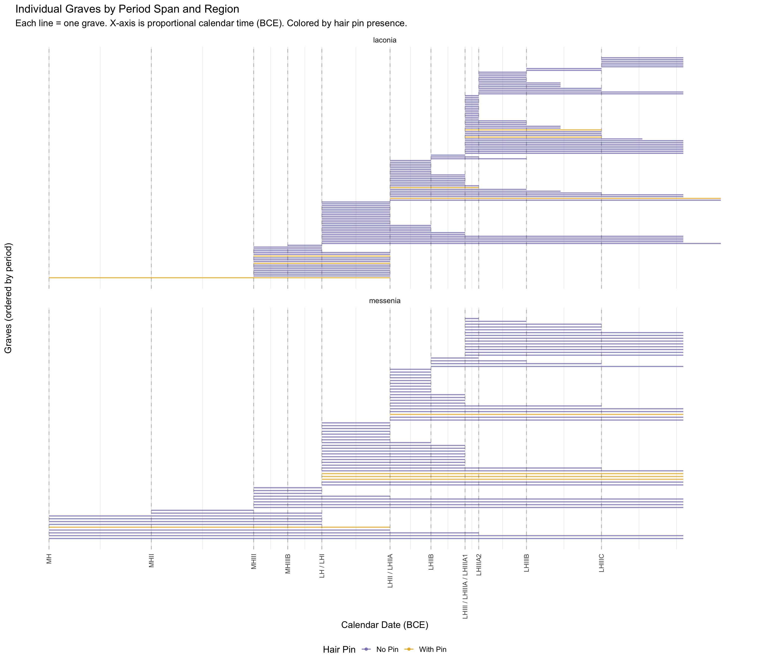
Chronological Classification

Period strings as recorded in the original dataset (e.g., “LHIIA,” “LHI–LHIII”) were matched against a period dictionary that assigns each code an earliest and latest component phase. Calendar date ranges were then attached by joining against a lookup table of BCE start and end dates for each component phase, based on conventional Aegean Bronze Age chronology. The period dictionary and calendar date table are loaded and applied below.

# NOTE: Set eval=TRUE once the student has completed the dictionaries

# Load period dictionary
period_dict <- read_csv(here::here("data", "period_dictionary.csv")) %>%
  mutate(across(where(is.character), str_trim))

# Load tomb type dictionary
tomb_dict <- read_csv(here::here("data", "tomb_type_dictionary.csv")) %>%
  mutate(tomb_type = str_trim(tomb_type))

# Join period dictionary and extract period components
cups_skulls_clean <- cups_skulls_clean %>%
  left_join(
    period_dict %>% select(period_code, chronological_order, earliest_component, latest_component),
    by = c("period" = "period_code")
  ) %>%

  # Get ordinal values for earliest component
  left_join(
    period_dict %>% select(period_code, chronological_order) %>% rename(start_order = chronological_order),
    by = c("earliest_component" = "period_code")
  ) %>%

  # Get ordinal values for latest component
  left_join(
    period_dict %>% select(period_code, chronological_order) %>% rename(end_order = chronological_order),
    by = c("latest_component" = "period_code")
  ) %>%

  # For single periods (where start = end), use that value
  # For ranges, create midpoint
  mutate(
    period_start_order = start_order,
    period_end_order = end_order,
    period_midpoint_order = (start_order + end_order) / 2
  )

# Calendar year lookup for each single-component period code
# Sources: user-supplied dates; sub-phases (MHIIIB, LHIIIB1, LHIIIC1) estimated
component_cal <- tribble(
  ~component,      ~cal_start_bce, ~cal_end_bce,
  "MH",            2000,           1600,
  "MHII",          1850,           1700,
  "MHIII",         1700,           1600,
  "MHIIIB",        1650,           1600,
  "LH",            1600,           1070,
  "LHI",           1600,           1500,
  "LHII",          1500,           1390,
  "LHIIA",         1500,           1440,
  "LHIIB",         1440,           1390,
  "LHIII",         1390,           1070,
  "LHIIIA",        1390,           1300,
  "LHIIIA1",       1390,           1370,
  "LHIIIA2",       1370,           1300,
  "LHIIIB",        1300,           1190,
  "LHIIIB1",       1300,           1250,
  "LHIIIC",        1190,           1070,
  "LHIIIC1",       1190,           1130,
  "submycenaean",  1070,           1015
)

# Add calendar year columns: start = start of earliest component,
# end = end of latest component
cups_skulls_clean <- cups_skulls_clean %>%
  left_join(
    component_cal %>% select(component, cal_start_bce),
    by = c("earliest_component" = "component")
  ) %>%
  rename(period_start_cal = cal_start_bce) %>%
  left_join(
    component_cal %>% select(component, cal_end_bce),
    by = c("latest_component" = "component")
  ) %>%
  rename(period_end_cal = cal_end_bce) %>%
  mutate(period_midpoint_cal = (period_start_cal + period_end_cal) / 2)

# Broad phase groupings with calendar spans for temporal plots
phase_cal <- tribble(
  ~broad_phase,  ~phase_start_bce, ~phase_end_bce,
  "MH",          2000,             1600,
  "LH I",        1600,             1500,
  "LH II",       1500,             1390,
  "LH IIIA",     1390,             1300,
  "LH IIIB",     1300,             1190,
  "LH IIIC",     1190,             1070,
  "SM",          1070,             1015
) %>% mutate(
  phase_mid_bce = (phase_start_bce + phase_end_bce) / 2,
  phase_duration = phase_start_bce - phase_end_bce,
  broad_phase = factor(broad_phase,
    levels = c("MH", "LH I", "LH II", "LH IIIA", "LH IIIB", "LH IIIC", "SM"),
    ordered = TRUE)
)

# Assign each grave to broadest phase based on its earliest component
cups_skulls_clean <- cups_skulls_clean %>%
  mutate(
    broad_phase = case_when(
      earliest_component %in% c("MH", "MHII", "MHIII", "MHIIIB") ~ "MH",
      earliest_component %in% c("LH", "LHI")                      ~ "LH I",
      earliest_component %in% c("LHII", "LHIIA", "LHIIB")         ~ "LH II",
      earliest_component %in% c("LHIII", "LHIIIA", "LHIIIA1", "LHIIIA2") ~ "LH IIIA",
      earliest_component %in% c("LHIIIB", "LHIIIB1")              ~ "LH IIIB",
      earliest_component %in% c("LHIIIC", "LHIIIC1")              ~ "LH IIIC",
      earliest_component == "submycenaean"                          ~ "SM",
      TRUE ~ NA_character_
    ),
    broad_phase = factor(broad_phase,
      levels = c("MH", "LH I", "LH II", "LH IIIA", "LH IIIB", "LH IIIC", "SM"),
      ordered = TRUE)
  )

# Map grave_type_simple names to tomb_type dictionary names
grave_to_tomb_map <- tibble(
  grave_type_simple = c("Tholos", "Chamber Tomb", "Cist Grave", "Pit Grave", "Dromos Only", "Other"),
  tomb_type_dict = c("tholos", "chamber tomb", "cist", "pit", "dromos of tholos", NA)
)

# Join tomb type dictionary via mapping
cups_skulls_clean <- cups_skulls_clean %>%
  left_join(grave_to_tomb_map, by = "grave_type_simple") %>%
  left_join(
    tomb_dict %>% select(tomb_type, tomb_type_order),
    by = c("tomb_type_dict" = "tomb_type")
  ) %>%
  select(-tomb_type_dict) %>%

  # Convert to ordered factors
  mutate(
    tomb_type_ordered = factor(
      grave_type_simple,
      levels = grave_to_tomb_map$grave_type_simple[
        order(tomb_dict$tomb_type_order[match(grave_to_tomb_map$tomb_type_dict, tomb_dict$tomb_type)])
      ],
      ordered = TRUE
    ),
    period_ordered = factor(
      period,
      levels = arrange(period_dict, chronological_order) %>% pull(period_code),
      ordered = TRUE
    )
  )

cat("✓ Dictionaries successfully loaded and applied!\n")
✓ Dictionaries successfully loaded and applied!
cat("New columns created:\n")
New columns created:
cat("  - period_start_order: chronological order of earliest period component\n")
  - period_start_order: chronological order of earliest period component
cat("  - period_end_order: chronological order of latest period component\n")
  - period_end_order: chronological order of latest period component
cat("  - period_midpoint_order: midpoint between start and end\n")
  - period_midpoint_order: midpoint between start and end
cat("  - tomb_type_ordered: ordered factor for tomb types\n")
  - tomb_type_ordered: ordered factor for tomb types
cat("  - period_ordered: ordered factor for periods\n")
  - period_ordered: ordered factor for periods

Data Overview

Basic Statistics

The table below summarizes overall dataset coverage and identifies variables with missing observations. Missing data reflect the state of the archaeological record and publication — not all excavated tombs have complete information on all variables — and are excluded from any calculation where the relevant variable is unknown.

cat("=== Dataset Summary ===\n\n")
=== Dataset Summary ===
cat("Total graves:", nrow(cups_skulls_clean), "\n")
Total graves: 296 
cat("Graves with drinking vessels recorded:", sum(cups_skulls_clean$has_drinking_vessel == TRUE, na.rm = TRUE), "\n")
Graves with drinking vessels recorded: 80 
cat("Graves with human remains:", sum(cups_skulls_clean$has_remains == TRUE, na.rm = TRUE), "\n")
Graves with human remains: 226 
cat("Graves with hair pins:", sum(cups_skulls_clean$has_pin == TRUE, na.rm = TRUE), "\n")
Graves with hair pins: 16 
cat("\n")
# Missing data summary
cat("=== Missing Data ===\n")
=== Missing Data ===
cups_skulls_clean %>%
  summarise(across(everything(), ~sum(is.na(.)))) %>%
  pivot_longer(everything(), names_to = "column", values_to = "missing_count") %>%
  dplyr::filter(missing_count > 0) %>%
  arrange(desc(missing_count)) %>%
  kable()
column missing_count
orientation 262
drinking_vessel_number 222
skulls_number 213
area_of_chamber_estimated 197
dimensions 171
end_order 104
period_end_order 104
period_midpoint_order 104
chronological_order 94
earliest_component 94
latest_component 94
start_order 94
period_start_order 94
period_start_cal 94
period_end_cal 94
period_midpoint_cal 94
broad_phase 94
period_ordered 94
period 90
tomb_type_order 37
type 12

Sites Represented

sites_summary <- cups_skulls_clean %>%
  count(site, region, name = "n_graves") %>%
  arrange(desc(n_graves))

cat("Number of sites:", n_distinct(cups_skulls_clean$site), "\n\n")
Number of sites: 50 
kable(sites_summary,
      col.names = c("Site", "Region", "Number of Graves"),
      caption = "Sites Represented in the Dataset") %>%
  kable_styling(bootstrap_options = c("striped", "hover", "condensed"))
Sites Represented in the Dataset
Site Region Number of Graves
Agios Stephanos laconia 63
volimidhia messenia 35
Xerokambi: Agios Vasileios North Cemetery laconia 25
Ayos Ioannis Papoulia messenia 23
Koukounara Gouvalari messenia 14
Epidavros Limera:PAL1 laconia 10
Peristeria & kokorakou messenia 9
Voidhokoloa messenia 9
Nihoria messenia 8
Handhrinou Kissos messenia 7
Kaminia messenia 7
Pellana laconia 7
Englianos messenia 6
Skoura: malathria laconia 6
Pellana: pelekete and Palaiokastro laconia 5
Peristeri: Solakos laconia 5
Routsi messenia 4
Sparti: Polydendron laconia 4
Sykea laconia 4
Amyklai: Spelakia laconia 3
Amyklaion laconia 3
Arkynes laconia 3
Geraki: Acropolis laconia 3
Daphi: Louria laconia 2
Daphni: Louria 3 laconia 2
Koukounara Livadhiti to Fities messenia 2
Koukounara akones messenia 2
Psari Metsiki messenia 2
Tragana messenia 2
Agios Georgios Voion laconia 1
Agios Vasileios: North Cemetery laconia 1
Angelona: Bastiza laconia 1
Dhara messenia 1
Epia Anthia messenia 1
Epidavros Limera laconia 1
Filiatra Stomion messenia 1
Kambos messenia 1
Kambos Voion laconia 1
Kaplani messenia 1
Kopanaki messenia 1
Korifasio messenia 1
Malthi messenia 1
Nisakouli (Methoni) messenia 1
Pila messenia 1
Solinari Tourlidhitsa messenia 1
Sparti: Psychiko laconia 1
Vapheio laconia 1
Vasiliko Xerovrisi messenia 1
Xerokambi: Agios Vasileios laconia 1
paleohoria messenia 1

Grave Type Distribution

Tomb types are compared across regions to establish the structural composition of each sample. Because tholos tombs, chamber tombs, cist graves, and pit graves represent different investments of labor and architectural elaboration, regional differences in tomb type distribution provide context for interpreting other patterns in the assemblage data.

grave_type_summary <- cups_skulls_clean %>%
  count(region, grave_type_simple, name = "count") %>%
  arrange(region, desc(count))

kable(grave_type_summary,
      col.names = c("Region", "Grave Type", "Count"),
      caption = "Grave Type Distribution by Region") %>%
  kable_styling(bootstrap_options = c("striped", "hover", "condensed"))
Grave Type Distribution by Region
Region Grave Type Count
laconia Cist Grave 63
laconia Chamber Tomb 44
laconia Pit Grave 22
laconia Other 18
laconia Tholos 6
messenia Tholos 50
messenia Chamber Tomb 38
messenia Pit Grave 25
messenia Other 19
messenia Cist Grave 11
grave_type_summary <- grave_type_summary %>%
  group_by(region) %>%
  mutate(pct = round(count / sum(count) * 100, 1)) %>%
  ungroup()

ggplot(grave_type_summary, aes(x = reorder(grave_type_simple, -count), y = count, fill = region)) +
  geom_col(position = "dodge", width = 0.7) +
  scale_fill_manual(values = c(laconia = colors$laconia, messenia = colors$messenia)) +
  geom_text(aes(label = paste0(count, "\n(", pct, "%)")), position = position_dodge(width = 0.7), vjust = -0.3, size = 3.5) +
  scale_y_continuous(expand = expansion(mult = c(0, 0.25))) +
  labs(
    title = "Distribution of Grave Types by Region",
    x = "Grave Type",
    y = "Number of Graves",
    fill = "Region"
  ) +
  theme_minimal(base_size = 16) +
  theme(legend.position = "bottom", axis.text.x = element_text(angle = 45, hjust = 1))

Version Author Date
7857fa6 tinalasisi 2026-03-10
01b0d46 tinalasisi 2026-02-17
8d3e1c7 tinalasisi 2026-02-17
2f9f6dc tinalasisi 2026-02-17

Burial Types

Primary vs Secondary Burials

Primary burial refers to the original, articulated interment of a body. Secondary burial refers to the later re-deposition of skeletal material — typically disarticulated bones that have been moved, often to make space for a subsequent interment. A single tomb can contain evidence for both. The distribution of these burial categories across regions is examined here as a baseline for later analyses that test whether drinking vessels and hair pins associate preferentially with one burial mode over another.

burial_type_summary <- cups_skulls_clean %>%
  summarise(
    total = n(),
    with_primary = sum(primary_burial == TRUE, na.rm = TRUE),
    with_secondary = sum(secondary_burial == TRUE, na.rm = TRUE),
    both = sum(primary_burial == TRUE & secondary_burial == TRUE, na.rm = TRUE),
    neither = sum(primary_burial == FALSE & secondary_burial == FALSE, na.rm = TRUE),
    unknown = sum(is.na(primary_burial) | is.na(secondary_burial))
  ) %>%
  mutate(
    pct_primary = round(with_primary / total * 100, 1),
    pct_secondary = round(with_secondary / total * 100, 1),
    pct_both = round(both / total * 100, 1)
  )

kable(burial_type_summary,
      col.names = c("Total", "With Primary", "With Secondary", "Both", "Neither", "Unknown",
                    "% Primary", "% Secondary", "% Both"),
      caption = "Primary vs Secondary Burial Summary") %>%
  kable_styling(bootstrap_options = c("striped", "hover", "condensed"))
Primary vs Secondary Burial Summary
Total With Primary With Secondary Both Neither Unknown % Primary % Secondary % Both
296 135 118 57 100 0 45.6 39.9 19.3
burial_category_data_region <- cups_skulls_clean %>%
  count(region, burial_category) %>%
  group_by(region) %>%
  mutate(pct = round(n / sum(n) * 100, 1)) %>%
  ungroup() %>%
  arrange(region, desc(n))

ggplot(burial_category_data_region, aes(x = reorder(burial_category, -n), y = n, fill = region)) +
  geom_col(position = "dodge", width = 0.7) +
  scale_fill_manual(values = c(laconia = colors$laconia, messenia = colors$messenia)) +
  geom_text(aes(label = paste0(n, "\n(", pct, "%)")), position = position_dodge(width = 0.7), vjust = -0.3, size = 3.5) +
  scale_y_continuous(expand = expansion(mult = c(0, 0.25))) +
  labs(
    title = "Distribution of Burial Types by Region",
    x = "Burial Type",
    y = "Count",
    fill = "Region"
  ) +
  theme_minimal(base_size = 16) +
  theme(legend.position = "bottom", axis.text.x = element_text(angle = 45, hjust = 1))

Version Author Date
7857fa6 tinalasisi 2026-03-10
01b0d46 tinalasisi 2026-02-17
8d3e1c7 tinalasisi 2026-02-17
2f9f6dc tinalasisi 2026-02-17

Drinking Vessels Analysis

Drinking vessels — cups, kylikes, and related forms — are among the most commonly recorded ceramic finds in Mycenaean funerary contexts and have been interpreted as indicators of feasting, libation, or other mortuary ritual. This section documents the prevalence of drinking vessels across the dataset, disaggregates that prevalence by tomb type and burial category, and compares patterns between Laconia and Messenia.

Overall Drinking Vessel Presence

dv_summary <- cups_skulls_clean %>%
  summarise(
    total_graves = n(),
    with_vessels = sum(has_drinking_vessel == TRUE, na.rm = TRUE),
    without_vessels = sum(has_drinking_vessel == FALSE, na.rm = TRUE),
    unknown_vessel_status = sum(is.na(has_drinking_vessel))
  ) %>%
  mutate(
    pct_with = round(with_vessels / total_graves * 100, 1),
    avg_vessels_recorded = round(mean(cups_skulls_clean$drinking_vessel_number, na.rm = TRUE), 2)
  )

kable(dv_summary,
      col.names = c("Total Graves", "With Vessels", "Without Vessels", "Unknown", "% With Vessels", "Avg Vessel Count"),
      caption = "Drinking Vessel Presence Summary") %>%
  kable_styling(bootstrap_options = c("striped", "hover", "condensed"))
Drinking Vessel Presence Summary
Total Graves With Vessels Without Vessels Unknown % With Vessels Avg Vessel Count
296 80 216 0 27 2.26

Drinking Vessels by Grave Type

dv_by_type <- cups_skulls_clean %>%
  group_by(grave_type_simple) %>%
  summarise(
    total = n(),
    with_vessels = sum(has_drinking_vessel == TRUE, na.rm = TRUE),
    pct_with_vessels = round(with_vessels / total * 100, 1),
    avg_vessel_count = round(mean(drinking_vessel_number, na.rm = TRUE), 2)
  ) %>%
  arrange(desc(with_vessels))

kable(dv_by_type,
      col.names = c("Grave Type", "Total Graves", "With Vessels", "% With Vessels", "Avg Vessel Count"),
      caption = "Drinking Vessels by Grave Type") %>%
  kable_styling(bootstrap_options = c("striped", "hover", "condensed"))
Drinking Vessels by Grave Type
Grave Type Total Graves With Vessels % With Vessels Avg Vessel Count
Chamber Tomb 82 38 46.3 2.62
Tholos 56 21 37.5 2.65
Pit Grave 47 8 17.0 1.14
Other 37 7 18.9 1.29
Cist Grave 74 6 8.1 1.33
dv_by_type_region <- cups_skulls_clean %>%
  group_by(region, grave_type_simple) %>%
  summarise(
    total = n(),
    with_vessels = sum(has_drinking_vessel == TRUE, na.rm = TRUE),
    pct_with_vessels = round(with_vessels / total * 100, 1),
    avg_vessel_count = round(mean(drinking_vessel_number, na.rm = TRUE), 2),
    .groups = "drop"
  ) %>%
  arrange(region, desc(with_vessels))

ggplot(dv_by_type_region, aes(x = reorder(grave_type_simple, -with_vessels), y = with_vessels, fill = region)) +
  geom_col(position = "dodge", width = 0.7) +
  scale_fill_manual(values = c(laconia = colors$laconia, messenia = colors$messenia)) +
  geom_text(aes(label = paste0(with_vessels, " (", pct_with_vessels, "%)")),
            position = position_dodge(width = 0.7), vjust = -0.3, size = 3.5) +
  scale_y_continuous(expand = expansion(mult = c(0, 0.2))) +
  labs(
    title = "Graves with Drinking Vessels by Grave Type and Region",
    x = "Grave Type",
    y = "Number of Graves with Drinking Vessels",
    fill = "Region"
  ) +
  theme_minimal(base_size = 16) +
  theme(legend.position = "bottom", axis.text.x = element_text(angle = 45, hjust = 1))

Version Author Date
7857fa6 tinalasisi 2026-03-10
01b0d46 tinalasisi 2026-02-17
8d3e1c7 tinalasisi 2026-02-17
2f9f6dc tinalasisi 2026-02-17

Drinking Vessels by Burial Type

dv_by_burial <- cups_skulls_clean %>%
  group_by(burial_category) %>%
  summarise(
    total = n(),
    with_vessels = sum(has_drinking_vessel == TRUE, na.rm = TRUE),
    pct_with_vessels = round(with_vessels / total * 100, 1),
    avg_vessel_count = round(mean(drinking_vessel_number, na.rm = TRUE), 2)
  ) %>%
  arrange(desc(with_vessels))

kable(dv_by_burial,
      col.names = c("Burial Type", "Total Graves", "With Vessels", "% With Vessels", "Avg Vessel Count"),
      caption = "Drinking Vessels by Burial Type") %>%
  kable_styling(bootstrap_options = c("striped", "hover", "condensed"))
Drinking Vessels by Burial Type
Burial Type Total Graves With Vessels % With Vessels Avg Vessel Count
Both Primary & Secondary 57 32 56.1 3.10
Secondary Only 61 20 32.8 1.83
Unknown/Not Recorded 100 19 19.0 1.88
Primary Only 78 9 11.5 1.00
dv_by_burial_region <- cups_skulls_clean %>%
  group_by(region, burial_category) %>%
  summarise(
    total = n(),
    with_vessels = sum(has_drinking_vessel == TRUE, na.rm = TRUE),
    pct_with_vessels = round(with_vessels / total * 100, 1),
    avg_vessel_count = round(mean(drinking_vessel_number, na.rm = TRUE), 2),
    .groups = "drop"
  ) %>%
  arrange(region, desc(with_vessels))

ggplot(dv_by_burial_region, aes(x = reorder(burial_category, -with_vessels), y = with_vessels, fill = region)) +
  geom_col(position = "dodge", width = 0.7) +
  scale_fill_manual(values = c(laconia = colors$laconia, messenia = colors$messenia)) +
  geom_text(aes(label = paste0(with_vessels, " (", pct_with_vessels, "%)")),
            position = position_dodge(width = 0.7), vjust = -0.3, size = 3.5) +
  scale_y_continuous(expand = expansion(mult = c(0, 0.2))) +
  labs(
    title = "Graves with Drinking Vessels by Burial Type and Region",
    x = "Burial Type",
    y = "Number of Graves with Drinking Vessels",
    fill = "Region"
  ) +
  theme_minimal(base_size = 16) +
  theme(legend.position = "bottom", axis.text.x = element_text(angle = 45, hjust = 1))

Version Author Date
7857fa6 tinalasisi 2026-03-10
01b0d46 tinalasisi 2026-02-17
8d3e1c7 tinalasisi 2026-02-17
2f9f6dc tinalasisi 2026-02-17

Hair Pin Analysis

Hair pins are personal ornaments found in a small subset of Laconian and Messenian graves. Their presence has been associated with female burials and with certain phases of the Bronze Age, though the sample is too small to support strong generalizations. This section documents overall hair pin prevalence and its regional distribution as a basis for the subsequent analyses examining co-occurrence with secondary burial, drinking vessels, and tomb size.

Overall Hair Pin Presence

pin_summary <- cups_skulls_clean %>%
  summarise(
    total_graves = n(),
    with_pins = sum(has_pin == TRUE, na.rm = TRUE),
    without_pins = sum(has_pin == FALSE, na.rm = TRUE),
    unknown_pin_status = sum(is.na(has_pin))
  ) %>%
  mutate(pct_with = round(with_pins / total_graves * 100, 1))

kable(pin_summary,
      col.names = c("Total Graves", "With Pins", "Without Pins", "Unknown", "% With Pins"),
      caption = "Hair Pin Presence Summary") %>%
  kable_styling(bootstrap_options = c("striped", "hover", "condensed"))
Hair Pin Presence Summary
Total Graves With Pins Without Pins Unknown % With Pins
296 16 280 0 5.4

Hair Pins by Region

pin_by_region <- cups_skulls_clean %>%
  group_by(region) %>%
  summarise(
    total = n(),
    with_pins = sum(has_pin == TRUE, na.rm = TRUE),
    pct_with_pins = round(with_pins / total * 100, 1),
    .groups = "drop"
  )

ggplot(pin_by_region, aes(x = region, y = with_pins, fill = region)) +
  geom_col(width = 0.6) +
  scale_fill_manual(values = c(laconia = colors$laconia, messenia = colors$messenia)) +
  geom_text(aes(label = paste0(with_pins, " (", pct_with_pins, "%)")), vjust = -0.3, size = 4) +
  scale_y_continuous(expand = expansion(mult = c(0, 0.2))) +
  labs(
    title = "Graves with Hair Pins by Region",
    x = "Region",
    y = "Number of Graves with Hair Pins",
    fill = "Region"
  ) +
  theme_minimal(base_size = 16) +
  theme(legend.position = "bottom")

Version Author Date
7857fa6 tinalasisi 2026-03-10

Secondary Burial and Hair Pins

Co-occurrence by Region

This section tests whether hair pins are more commonly found in graves with evidence of secondary burial. If pins are associated with specific individuals whose remains were later moved or disturbed, they might be expected to cluster with secondary contexts. Conversely, if pins are associated with the initial primary interment, they might appear more often in graves without secondary activity.

Because the sample of pin-bearing graves is small (n = 16 total), conventional chi-square tests would violate the assumption of adequate cell counts. Fisher’s exact test is used instead, as it is appropriate for contingency tables with small expected frequencies. Results are reported separately for each region.

secondary_pins <- cups_skulls_clean %>%
  dplyr::filter(!is.na(secondary_burial) & !is.na(has_pin)) %>%
  group_by(region, secondary_burial, has_pin) %>%
  summarise(count = n(), .groups = "drop") %>%
  mutate(
    secondary_label = ifelse(secondary_burial, "Secondary Present", "Secondary Absent"),
    pin_label = ifelse(has_pin, "With Pin", "No Pin")
  )

# Summary table
secondary_pins_wide <- secondary_pins %>%
  select(region, secondary_label, pin_label, count) %>%
  pivot_wider(names_from = pin_label, values_from = count, values_fill = 0)

kable(secondary_pins_wide)
region secondary_label No Pin With Pin
laconia Secondary Absent 93 4
laconia Secondary Present 53 3
messenia Secondary Absent 76 5
messenia Secondary Present 58 4
secondary_pins_pct <- cups_skulls_clean %>%
  dplyr::filter(!is.na(secondary_burial) & !is.na(has_pin)) %>%
  group_by(region, secondary_burial) %>%
  summarise(
    total = n(),
    with_pin = sum(has_pin == TRUE),
    pct_with_pin = round(with_pin / total * 100, 1),
    .groups = "drop"
  ) %>%
  mutate(secondary_label = ifelse(secondary_burial, "Secondary Present", "Secondary Absent"))

ggplot(secondary_pins_pct, aes(x = secondary_label, y = pct_with_pin, fill = region)) +
  geom_col(position = "dodge", width = 0.7) +
  scale_fill_manual(values = c(laconia = colors$laconia, messenia = colors$messenia)) +
  geom_text(aes(label = paste0(with_pin, "/", total, "\n(", pct_with_pin, "%)")),
            position = position_dodge(width = 0.7), vjust = -0.3, size = 3.5) +
  scale_y_continuous(expand = expansion(mult = c(0, 0.25))) +
  labs(
    title = "Hair Pin Presence by Secondary Burial Status and Region",
    x = "Secondary Burial Status",
    y = "% of Graves with Hair Pins",
    fill = "Region"
  ) +
  theme_minimal(base_size = 16) +
  theme(legend.position = "bottom")

Version Author Date
7857fa6 tinalasisi 2026-03-10
# Fisher's exact test by region (appropriate for small cell counts)
for (reg in unique(cups_skulls_clean$region)) {
  region_data <- cups_skulls_clean %>%
    dplyr::filter(region == reg & !is.na(secondary_burial) & !is.na(has_pin))

  contingency <- table(region_data$secondary_burial, region_data$has_pin)

  cat("\n===", toupper(reg), "===\n")
  print(kable(as.data.frame.matrix(contingency),
              caption = paste("Contingency Table:", toupper(reg))) %>%
    kable_styling(bootstrap_options = c("striped", "hover", "condensed")))

  if (all(dim(contingency) == c(2, 2))) {
    fisher_result <- fisher.test(contingency)
    cat("Fisher's exact test p-value:", round(fisher_result$p.value, 4), "\n")
    cat("Odds ratio:", round(fisher_result$estimate, 3), "\n")
  } else {
    cat("Insufficient variation for statistical test\n")
  }
}

=== LACONIA ===
<table class="table table-striped table-hover table-condensed" style="margin-left: auto; margin-right: auto;">
<caption>Contingency Table: LACONIA</caption>
 <thead>
  <tr>
   <th style="text-align:left;">  </th>
   <th style="text-align:right;"> FALSE </th>
   <th style="text-align:right;"> TRUE </th>
  </tr>
 </thead>
<tbody>
  <tr>
   <td style="text-align:left;"> FALSE </td>
   <td style="text-align:right;"> 93 </td>
   <td style="text-align:right;"> 4 </td>
  </tr>
  <tr>
   <td style="text-align:left;"> TRUE </td>
   <td style="text-align:right;"> 53 </td>
   <td style="text-align:right;"> 3 </td>
  </tr>
</tbody>
</table>Fisher's exact test p-value: 0.7071 
Odds ratio: 1.314 

=== MESSENIA ===
<table class="table table-striped table-hover table-condensed" style="margin-left: auto; margin-right: auto;">
<caption>Contingency Table: MESSENIA</caption>
 <thead>
  <tr>
   <th style="text-align:left;">  </th>
   <th style="text-align:right;"> FALSE </th>
   <th style="text-align:right;"> TRUE </th>
  </tr>
 </thead>
<tbody>
  <tr>
   <td style="text-align:left;"> FALSE </td>
   <td style="text-align:right;"> 76 </td>
   <td style="text-align:right;"> 5 </td>
  </tr>
  <tr>
   <td style="text-align:left;"> TRUE </td>
   <td style="text-align:right;"> 58 </td>
   <td style="text-align:right;"> 4 </td>
  </tr>
</tbody>
</table>Fisher's exact test p-value: 1 
Odds ratio: 1.048 

Drinking Vessels, Secondary Burial, and Hair Pins

Three-Way Cross-Tabulation by Region

To examine whether drinking vessels, secondary burial, and hair pins co-occur beyond chance, a three-way cross-tabulation is constructed separately for each region. This allows identification of any combinations of these three variables that appear disproportionately often or rarely. Given the small total number of pin-bearing graves, this analysis is primarily descriptive; cell counts are reported alongside the visualization.

three_way <- cups_skulls_clean %>%
  dplyr::filter(!is.na(has_drinking_vessel) & !is.na(secondary_burial) & !is.na(has_pin)) %>%
  group_by(region, has_drinking_vessel, secondary_burial, has_pin) %>%
  summarise(count = n(), .groups = "drop") %>%
  mutate(
    vessel_label = ifelse(has_drinking_vessel, "Vessel Present", "No Vessel"),
    secondary_label = ifelse(secondary_burial, "Secondary Present", "Secondary Absent"),
    pin_label = ifelse(has_pin, "With Pin", "No Pin")
  )

kable(three_way %>% select(region, vessel_label, secondary_label, pin_label, count))
region vessel_label secondary_label pin_label count
laconia No Vessel Secondary Absent No Pin 84
laconia No Vessel Secondary Absent With Pin 2
laconia No Vessel Secondary Present No Pin 36
laconia No Vessel Secondary Present With Pin 2
laconia Vessel Present Secondary Absent No Pin 9
laconia Vessel Present Secondary Absent With Pin 2
laconia Vessel Present Secondary Present No Pin 17
laconia Vessel Present Secondary Present With Pin 1
messenia No Vessel Secondary Absent No Pin 63
messenia No Vessel Secondary Absent With Pin 1
messenia No Vessel Secondary Present No Pin 28
messenia Vessel Present Secondary Absent No Pin 13
messenia Vessel Present Secondary Absent With Pin 4
messenia Vessel Present Secondary Present No Pin 30
messenia Vessel Present Secondary Present With Pin 4
three_way_summary <- cups_skulls_clean %>%
  dplyr::filter(!is.na(has_drinking_vessel) & !is.na(secondary_burial) & !is.na(has_pin)) %>%
  mutate(
    vessel_label = ifelse(has_drinking_vessel, "Vessel Present", "No Vessel"),
    secondary_label = ifelse(secondary_burial, "Secondary Present", "Secondary Absent"),
    pin_label = ifelse(has_pin, "With Pin", "No Pin")
  ) %>%
  count(region, vessel_label, secondary_label, pin_label)

ggplot(three_way_summary, aes(x = secondary_label, y = n, fill = pin_label)) +
  geom_col(position = "dodge", width = 0.7) +
  scale_fill_manual(values = c("With Pin" = colors$pin, "No Pin" = "grey70")) +
  facet_grid(vessel_label ~ region) +
  geom_text(aes(label = n), position = position_dodge(width = 0.7), vjust = -0.3, size = 3) +
  scale_y_continuous(expand = expansion(mult = c(0, 0.2))) +
  labs(
    title = "Hair Pins by Secondary Burial Status and Drinking Vessel Presence",
    subtitle = "Rows: Drinking Vessel status | Columns: Region",
    x = "Secondary Burial Status",
    y = "Count",
    fill = "Hair Pin"
  ) +
  theme_minimal(base_size = 16) +
  theme(legend.position = "bottom", axis.text.x = element_text(angle = 45, hjust = 1))

Version Author Date
7857fa6 tinalasisi 2026-03-10

Hair Pins and Chamber Size

Larger tomb chambers may reflect greater investment in funerary architecture, which could correlate with higher-status or more elaborately furnished burials. This section examines whether graves containing hair pins have systematically larger estimated chamber areas than those without. Chamber area is available for a subset of graves and is expressed in estimated square meters.

Because chamber area distributions are right-skewed and may not be normally distributed, a non-parametric Wilcoxon rank-sum test is used to compare the distributions of chamber area between pin-bearing and non-pin-bearing graves within each region. Boxplots are provided to visualize the distributions directly.

Chamber Area by Hair Pin Presence

pins_area_data <- cups_skulls_clean %>%
  dplyr::filter(!is.na(area_of_chamber_estimated) & !is.na(has_pin))

cat("Graves with area AND pin status:", nrow(pins_area_data), "\n")
Graves with area AND pin status: 99 
pins_area_data %>%
  group_by(has_pin) %>%
  summarise(
    n = n(),
    mean_area = round(mean(area_of_chamber_estimated, na.rm = TRUE), 2),
    median_area = round(median(area_of_chamber_estimated, na.rm = TRUE), 2),
    sd_area = round(sd(area_of_chamber_estimated, na.rm = TRUE), 2),
    .groups = "drop"
  ) %>%
  mutate(pin_label = ifelse(has_pin, "With Pin", "No Pin")) %>%
  kable()
has_pin n mean_area median_area sd_area pin_label
FALSE 92 18.41 12.26 17.89 No Pin
TRUE 7 27.57 22.90 26.72 With Pin
ggplot(pins_area_data, aes(x = ifelse(has_pin, "With Pin", "No Pin"),
                            y = area_of_chamber_estimated, fill = region)) +
  geom_boxplot(alpha = 0.7, position = "dodge") +
  scale_fill_manual(values = c(laconia = colors$laconia, messenia = colors$messenia)) +
  labs(
    title = "Chamber Area by Hair Pin Presence and Region",
    x = "Hair Pin Status",
    y = "Chamber Area Estimated (m\u00b2)",
    fill = "Region"
  ) +
  theme_minimal(base_size = 16) +
  theme(legend.position = "bottom")

Version Author Date
7857fa6 tinalasisi 2026-03-10
# Wilcoxon test (non-parametric, appropriate for potentially non-normal area data)
for (reg in unique(pins_area_data$region)) {
  region_data <- pins_area_data %>% dplyr::filter(region == reg)
  with_pin <- region_data %>% dplyr::filter(has_pin == TRUE) %>% pull(area_of_chamber_estimated)
  without_pin <- region_data %>% dplyr::filter(has_pin == FALSE) %>% pull(area_of_chamber_estimated)

  cat("\n===", toupper(reg), "===\n")
  cat("With pin: n =", length(with_pin), ", median =", round(median(with_pin), 2), "\n")
  cat("Without pin: n =", length(without_pin), ", median =", round(median(without_pin), 2), "\n")

  if (length(with_pin) >= 2 & length(without_pin) >= 2) {
    test_result <- wilcox.test(with_pin, without_pin)
    cat("Wilcoxon rank-sum test p-value:", round(test_result$p.value, 4), "\n")
  } else {
    cat("Too few observations for statistical test\n")
  }
}

=== LACONIA ===
With pin: n = 2 , median = 56.2 
Without pin: n = 29 , median = 8.58 
Wilcoxon rank-sum test p-value: 0.0258 

=== MESSENIA ===
With pin: n = 5 , median = 19.64 
Without pin: n = 63 , median = 12.57 
Wilcoxon rank-sum test p-value: 0.8786 

Skeletal Remains Analysis

The presence of identifiable human remains — particularly skulls, which are the most commonly recorded skeletal element — provides a partial window into how many individuals were interred and whether bones were disturbed or removed. This section describes overall remains prevalence and skull counts, which are used in subsequent analyses of the relationship between drinking vessels and the physical presence of the dead.

Remains Distribution

remains_summary <- cups_skulls_clean %>%
  summarise(
    total_graves = n(),
    with_remains = sum(has_remains == TRUE, na.rm = TRUE),
    without_remains = sum(has_remains == FALSE, na.rm = TRUE),
    unknown_remains = sum(is.na(has_remains))
  ) %>%
  mutate(pct_with_remains = round(with_remains / total_graves * 100, 1))

kable(remains_summary,
      col.names = c("Total Graves", "With Remains", "Without Remains", "Unknown", "% With Remains"),
      caption = "Skeletal Remains Presence Summary") %>%
  kable_styling(bootstrap_options = c("striped", "hover", "condensed"))
Skeletal Remains Presence Summary
Total Graves With Remains Without Remains Unknown % With Remains
296 226 70 0 76.4

Skulls Recorded

skulls_stats <- cups_skulls_clean %>%
  dplyr::filter(!is.na(skulls_number)) %>%
  summarise(
    graves_with_skull_count = n(),
    total_skulls = sum(skulls_number, na.rm = TRUE),
    avg_skulls = round(mean(skulls_number, na.rm = TRUE), 2),
    min_skulls = min(skulls_number, na.rm = TRUE),
    max_skulls = max(skulls_number, na.rm = TRUE)
  )

kable(skulls_stats,
      col.names = c("Graves with Skull Count", "Total Skulls", "Avg Skulls", "Min", "Max"),
      caption = "Skull Count Statistics") %>%
  kable_styling(bootstrap_options = c("striped", "hover", "condensed"))
Skull Count Statistics
Graves with Skull Count Total Skulls Avg Skulls Min Max
83 350 4.22 1 47
skulls_by_count <- cups_skulls_clean %>%
  dplyr::filter(!is.na(skulls_number)) %>%
  count(skulls_number, name = "graves") %>%
  arrange(skulls_number)

kable(skulls_by_count,
      col.names = c("Skulls Recorded", "Number of Graves"),
      caption = "Distribution of Skull Counts per Grave") %>%
  kable_styling(bootstrap_options = c("striped", "hover", "condensed"))
Distribution of Skull Counts per Grave
Skulls Recorded Number of Graves
1 48
2 10
3 5
4 2
5 1
6 3
7 1
9 2
10 2
12 2
14 1
15 1
20 2
24 1
27 1
47 1

Drinking Vessels and Skeletal Remains

A central question for this thesis is whether drinking vessels are more likely to be deposited when human remains are present in the tomb — suggesting a direct relationship between the objects and the body — or whether they appear regardless of skeletal preservation. This section cross-tabulates drinking vessel presence against skeletal remains presence, and examines whether the number of drinking vessels correlates with the number of skulls recorded (as a proxy for the number of individuals interred).

Drinking Vessel Presence and Remains Co-occurrence

vessels_remains_cross <- cups_skulls_clean %>%
  dplyr::filter(!is.na(has_drinking_vessel) & !is.na(has_remains)) %>%
  count(has_drinking_vessel, has_remains) %>%
  pivot_wider(names_from = has_remains, values_from = n, values_fill = 0) %>%
  rename(no_remains = `FALSE`, with_remains = `TRUE`)

vessels_remains_cross <- vessels_remains_cross %>%
  mutate(vessel_status = ifelse(has_drinking_vessel, "With Drinking Vessels", "No Drinking Vessels")) %>%
  select(vessel_status, no_remains, with_remains)

kable(vessels_remains_cross,
      col.names = c("Vessel Status", "No Remains", "With Remains"),
      caption = "Cross-Tabulation: Drinking Vessels and Skeletal Remains") %>%
  kable_styling(bootstrap_options = c("striped", "hover", "condensed"))
Cross-Tabulation: Drinking Vessels and Skeletal Remains
Vessel Status No Remains With Remains
No Drinking Vessels 55 161
With Drinking Vessels 15 65
# Calculate cross-tabulation with percentages
cross_analysis <- cups_skulls_clean %>%
  dplyr::filter(!is.na(has_drinking_vessel) & !is.na(has_remains)) %>%
  group_by(has_drinking_vessel) %>%
  summarise(
    total = n(),
    with_remains = sum(has_remains == TRUE, na.rm = TRUE),
    pct_with_remains = round(with_remains / total * 100, 1)
  ) %>%
  mutate(vessel_status = ifelse(has_drinking_vessel, "With Drinking Vessels", "Without Drinking Vessels"))

kable(select(cross_analysis, vessel_status, total, with_remains, pct_with_remains))
vessel_status total with_remains pct_with_remains
Without Drinking Vessels 216 161 74.5
With Drinking Vessels 80 65 81.2

Drinking Vessels and Skull Count

vessels_skulls_data <- cups_skulls_clean %>%
  dplyr::filter(!is.na(drinking_vessel_number) & !is.na(skulls_number)) %>%
  mutate(has_vessels_label = ifelse(has_drinking_vessel, "With Vessels", "No Vessels"))

ggplot(vessels_skulls_data, aes(x = drinking_vessel_number, y = skulls_number, color = has_vessels_label)) +
  geom_jitter(size = 3, alpha = 0.6, width = 0.2, height = 0.2) +
  geom_smooth(method = "lm", se = FALSE, alpha = 0.2) +
  labs(
    title = "Relationship: Drinking Vessels vs Skull Count",
    x = "Number of Drinking Vessels Recorded",
    y = "Number of Skulls",
    color = ""
  ) +
  theme_minimal(base_size = 16) +
  theme(legend.position = "bottom")

Version Author Date
7857fa6 tinalasisi 2026-03-10
2f9f6dc tinalasisi 2026-02-17

Regional Comparison

This section brings together the key assemblage variables into a single regional summary, directly comparing Laconia and Messenia on drinking vessel prevalence, skeletal remains presence, and average skull count per grave. Differences between regions are relevant for interpreting whether patterns observed in the full dataset are driven primarily by one region or reflect a broader Mycenaean phenomenon.

Summary by Region

regional_summary <- cups_skulls_clean %>%
  group_by(region) %>%
  summarise(
    total_graves = n(),
    with_drinking_vessels = sum(has_drinking_vessel == TRUE, na.rm = TRUE),
    pct_with_vessels = round(with_drinking_vessels / total_graves * 100, 1),
    with_remains = sum(has_remains == TRUE, na.rm = TRUE),
    pct_with_remains = round(with_remains / total_graves * 100, 1),
    avg_skulls = round(mean(skulls_number, na.rm = TRUE), 2)
  )

kable(regional_summary,
      col.names = c("Region", "Total Graves", "With Drinking Vessels", "% With Vessels",
                    "With Remains", "% With Remains", "Avg Skulls"),
      caption = "Regional Summary: Drinking Vessels and Skeletal Remains") %>%
  kable_styling(bootstrap_options = c("striped", "hover", "condensed"))
Regional Summary: Drinking Vessels and Skeletal Remains
Region Total Graves With Drinking Vessels % With Vessels With Remains % With Remains Avg Skulls
laconia 153 29 19.0 127 83.0 2.22
messenia 143 51 35.7 99 69.2 6.17

Chronological Overview

Periods Represented in the Dataset

Graves in this dataset carry period attributions that range in precision from a single sub-phase (e.g., “LHIIIA2”) to broad spans covering several centuries (e.g., “MH–LHIIIC”). The table below summarizes how many graves fall into broad period categories. Graves with no recorded period are retained in all non-temporal analyses but excluded from analyses that require chronological assignment.

period_summary <- cups_skulls_clean %>%
  mutate(
    period_category = case_when(
      str_detect(tolower(period), "mh") ~ "Middle Helladic",
      str_detect(tolower(period), "lh\\s*i(?!i)")  | str_detect(tolower(period), "lh i-") ~ "LH I-II",
      str_detect(tolower(period), "lh\\s*ii") & !str_detect(tolower(period), "lh\\s*ii") ~ "LH II",
      str_detect(tolower(period), "lh\\s*iii") ~ "LH III",
      str_detect(tolower(period), "lh") ~ "Late Helladic (general)",
      is.na(period) | period == "" ~ "Unrecorded",
      TRUE ~ "Other"
    )
  ) %>%
  count(period_category, name = "graves") %>%
  arrange(desc(graves))

kable(period_summary,
      col.names = c("Period Category", "Number of Graves"),
      caption = "Graves by Period Category") %>%
  kable_styling(bootstrap_options = c("striped", "hover", "condensed"))
Graves by Period Category
Period Category Number of Graves
Unrecorded 90
LH III 88
LH I-II 45
Middle Helladic 39
Late Helladic (general) 34

Period Span Analysis

The chart below maps each period code used in the dataset onto the Bronze Age calendar. The x-axis is proportional to actual calendar years (BCE), making the width of each row a direct representation of chronological uncertainty. Range periods (e.g., “LHIIA–LHIIIB”) appear as horizontal segments; single-phase codes (e.g., “LHIIIA2”) appear as points. Dashed vertical lines mark the start of each major phase; tick labels that combine multiple codes (e.g., “LHIII / LHIIIA / LHIIIA1”) reflect phases whose calendar start dates coincide.

This visualization is intended to make the degree of chronological imprecision in the dataset transparent before the temporal analyses that follow.

# Identify single-component periods and attach calendar years
single_periods <- period_dict %>%
  dplyr::filter(earliest_component == latest_component) %>%
  select(period_code, chronological_order) %>%
  arrange(chronological_order) %>%
  distinct(period_code, .keep_all = TRUE) %>%
  dplyr::filter(period_code != "LH II") %>%
  left_join(component_cal %>% select(component, cal_start_bce),
            by = c("period_code" = "component"))

# Get all period codes in the data with their calendar year spans
period_spans <- cups_skulls_clean %>%
  dplyr::filter(!is.na(period_start_cal) & !is.na(period_end_cal)) %>%
  distinct(period, period_start_cal, period_end_cal) %>%
  mutate(
    is_range = period_start_cal != period_end_cal,
    span_width = period_start_cal - period_end_cal  # BCE: larger start = earlier
  ) %>%
  arrange(desc(period_start_cal), period_end_cal)

# Count graves per period code
period_counts <- cups_skulls_clean %>%
  dplyr::filter(!is.na(period_start_cal)) %>%
  count(period, name = "n_graves")

period_spans <- period_spans %>%
  left_join(period_counts, by = "period") %>%
  mutate(period_label = paste0(period, " (n=", n_graves, ")")) %>%
  mutate(period_label = factor(period_label,
    levels = rev(mutate(arrange(., desc(period_start_cal), period_end_cal),
                        period_label = paste0(period, " (n=", n_graves, ")"))$period_label)))

# Collapse period codes that share the same calendar position into one label
# (e.g. LH and LHI both start at 1600 BCE — combine as "LH / LHI")
single_periods_unique <- dplyr::filter(single_periods, !is.na(cal_start_bce)) %>%
  group_by(cal_start_bce) %>%
  summarise(period_code = paste(period_code, collapse = " / "), .groups = "drop")

ggplot(period_spans) +
  geom_segment(
    data = dplyr::filter(period_spans, is_range),
    aes(x = period_start_cal, xend = period_end_cal,
        y = period_label, yend = period_label),
    linewidth = 2, color = colors$drinking_vessel, alpha = 0.7
  ) +
  geom_point(
    aes(x = period_start_cal, y = period_label),
    size = 3, color = colors$drinking_vessel
  ) +
  geom_point(
    data = dplyr::filter(period_spans, is_range),
    aes(x = period_end_cal, y = period_label),
    size = 3, color = colors$drinking_vessel
  ) +
  geom_vline(
    data = single_periods_unique,
    aes(xintercept = cal_start_bce),
    linetype = "dashed", alpha = 0.3
  ) +
  scale_x_reverse(
    breaks = single_periods_unique$cal_start_bce,
    labels = single_periods_unique$period_code
  ) +
  labs(
    title = "Period Spans in the Dataset",
    subtitle = "Each row is a period code used in the data. X-axis is proportional calendar time (BCE).",
    x = "Calendar Date (BCE)",
    y = "Period Code (n = number of graves)"
  ) +
  theme_minimal(base_size = 14) +
  theme(
    axis.text.x = element_text(angle = 90, hjust = 1, vjust = 0.5, size = 10),
    axis.text.y = element_text(size = 9),
    panel.grid.major.y = element_line(color = "grey90"),
    panel.grid.minor = element_blank()
  )

Version Author Date
7857fa6 tinalasisi 2026-03-10
cat("=== Individual chronological components (in order) ===\n\n")
=== Individual chronological components (in order) ===
for (i in 1:nrow(single_periods)) {
  cat(sprintf("  %2d. %s\n", i, single_periods$period_code[i]))
}
   1. MH
   2. MHII
   3. MHIII
   4. MHIIIB
   5. LH
   6. LHI
   7. LHII
   8. LHIIA
   9. LHIIB
  10. LHIII
  11. LHIIIA
  12. LHIIIA1
  13. LHIIIA2
  14. LHIIIB
  15. LHIIIC
cat("\n=== Summary ===\n")

=== Summary ===
cat("Single-period codes:", sum(!period_spans$is_range), "\n")
Single-period codes: 0 
cat("Range-period codes:", sum(period_spans$is_range), "\n")
Range-period codes: 55 
cat("Total period codes in data:", nrow(period_spans), "\n")
Total period codes in data: 55 
cat("\n=== Range periods spanning 3+ components ===\n")

=== Range periods spanning 3+ components ===
wide_spans <- period_spans %>%
  dplyr::filter(span_width > 10) %>%
  arrange(desc(span_width))
if (nrow(wide_spans) > 0) {
  for (i in 1:nrow(wide_spans)) {
    cat(sprintf("  %s: spans from order %g to %g (width = %g, n = %d graves)\n",
        wide_spans$period[i], wide_spans$period_start_order[i],
        wide_spans$period_end_order[i], wide_spans$span_width[i],
        wide_spans$n_graves[i]))
  }
}

Individual Graves by Period Span and Region

Each line represents a single grave plotted against calendar time, spanning its full attributed date range. Graves are colored by hair pin presence, allowing visual inspection of whether pin-bearing graves are concentrated in particular periods or distributed broadly across the sequence. Graves without datable period codes are excluded.

# Prepare individual grave data with calendar year spans
graves_time <- cups_skulls_clean %>%
  dplyr::filter(!is.na(period_start_cal) & !is.na(period_end_cal) & !is.na(has_pin)) %>%
  mutate(pin_label = ifelse(has_pin, "With Pin", "No Pin")) %>%
  # Order graves: earlier start first (higher BCE = earlier), then narrower range
  arrange(region, desc(period_start_cal), period_end_cal) %>%
  group_by(region) %>%
  mutate(grave_rank = row_number()) %>%
  ungroup()

# Reuse the deduplicated tick table built in the period-span-chart chunk
# (collapses codes sharing the same calendar position, e.g. "LHIII / LHIIIA / LHIIIA1")

ggplot(graves_time) +
  geom_segment(
    aes(x = period_start_cal, xend = period_end_cal,
        y = grave_rank, yend = grave_rank,
        color = pin_label),
    linewidth = 0.8, alpha = 0.7
  ) +
  geom_point(
    data = dplyr::filter(graves_time, period_start_cal == period_end_cal),
    aes(x = period_start_cal, y = grave_rank, color = pin_label),
    size = 1.5, alpha = 0.7
  ) +
  scale_color_manual(values = c("With Pin" = colors$pin, "No Pin" = colors$drinking_vessel)) +
  geom_vline(
    data = single_periods_unique,
    aes(xintercept = cal_start_bce),
    linetype = "dashed", alpha = 0.2
  ) +
  scale_x_reverse(
    breaks = single_periods_unique$cal_start_bce,
    labels = single_periods_unique$period_code
  ) +
  facet_wrap(~region, ncol = 1, scales = "free_y") +
  labs(
    title = "Individual Graves by Period Span and Region",
    subtitle = "Each line = one grave. X-axis is proportional calendar time (BCE). Colored by hair pin presence.",
    x = "Calendar Date (BCE)",
    y = "Graves (ordered by period)",
    color = "Hair Pin"
  ) +
  theme_minimal(base_size = 14) +
  theme(
    legend.position = "bottom",
    axis.text.x = element_text(angle = 90, hjust = 1, vjust = 0.5, size = 10),
    axis.text.y = element_blank(),
    axis.ticks.y = element_blank(),
    panel.grid.major.y = element_blank(),
    panel.grid.minor.y = element_blank()
  )

Version Author Date
3216d85 tinalasisi 2026-03-10
7857fa6 tinalasisi 2026-03-10

Temporal Analyses

These analyses examine whether funerary practices — burial type, drinking vessel presence, hair pin presence, and tomb size — changed over the course of the Bronze Age, and whether any such changes differed between Laconia and Messenia.

Phase Assignment

Because most graves carry date ranges rather than precise phase attributions, each grave is assigned to a broad phase based on the earliest component of its recorded period. A grave dated “LHIIA–LHIIIB,” for instance, is counted in the LH II phase. This is a conservative choice: it avoids assigning a grave to a later phase it may not actually represent, but it means that graves with wide date ranges are anchored at their earliest possible position. Any apparent trends toward earlier phases should be read with this in mind.

Seven broad phases are used: MH, LH I, LH II, LH III, LH IIIA, LH IIIB, and LH IIIC/Submycenaean. Graves whose period code could not be matched to any known component receive NA and are excluded from all temporal plots. Graves recorded only as the undifferentiated “LH” code are assigned to LH I.

Each temporal plot is shown in two versions: Option A uses an ordered categorical x-axis with equal spacing between phases; Option B uses a proportional calendar x-axis where bar widths are scaled to actual phase duration in calendar years. Option B better represents the unequal lengths of the phases but can be harder to read when phases have few graves.

phase_table <- as.data.frame(table(cups_skulls_clean$broad_phase, useNA = "ifany"))
names(phase_table) <- c("Broad Phase", "Number of Graves")
kable(phase_table, caption = "Graves Assigned to Broad Phases") %>%
  kable_styling(bootstrap_options = c("striped", "hover", "condensed"))
Graves Assigned to Broad Phases
Broad Phase Number of Graves
MH 38
LH I 47
LH II 49
LH IIIA 60
LH IIIB 2
LH IIIC 6
SM 0
NA 94

Burial Type Composition Over Time

These charts track whether the proportion of primary-only, secondary-only, mixed, and unrecorded burials changed across the Bronze Age sequence within each region. Stacked bars represent 100% of graves assigned to each phase, so the chart shows relative composition rather than absolute counts. The “Neither/Unknown” category reflects graves for which burial type was not recorded in the published sources; its size in any given phase indicates the limits of the available evidence for that period rather than the absence of burials.

Option A: Broad Phase Categories — Proportions

burial_cat_data <- cups_skulls_clean %>%
  dplyr::filter(!is.na(broad_phase)) %>%
  mutate(burial_cat = case_when(
    primary_burial == TRUE & secondary_burial == TRUE ~ "Both",
    primary_burial == TRUE                            ~ "Primary only",
    secondary_burial == TRUE                          ~ "Secondary only",
    TRUE                                              ~ "Neither/Unknown"
  ),
  burial_cat = factor(burial_cat,
    levels = c("Primary only", "Both", "Secondary only", "Neither/Unknown"))) %>%
  group_by(region, broad_phase, burial_cat) %>%
  summarise(n = n(), .groups = "drop") %>%
  group_by(region, broad_phase) %>%
  mutate(total = sum(n), pct = n / total * 100) %>%
  ungroup()

phase_totals_burial <- burial_cat_data %>%
  distinct(region, broad_phase, total)

ggplot(burial_cat_data, aes(x = broad_phase, y = pct, fill = burial_cat)) +
  geom_col(position = "stack", width = 0.7) +
  geom_text(aes(label = ifelse(pct >= 8, paste0(round(pct), "%"), "")),
            position = position_stack(vjust = 0.5), size = 3.5, color = "white") +
  geom_text(data = phase_totals_burial,
            aes(x = broad_phase, y = 104, label = paste0("n=", total)),
            inherit.aes = FALSE, vjust = 0, size = 3.5) +
  scale_fill_manual(values = c(
    "Primary only"    = colors$drinking_vessel,
    "Both"            = "#44AA99",
    "Secondary only"  = colors$skulls,
    "Neither/Unknown" = "grey80"
  )) +
  scale_y_continuous(limits = c(0, 113), labels = function(x) paste0(x, "%")) +
  facet_wrap(~region, ncol = 1) +
  labs(
    title = "Burial Type Composition Over Time by Region",
    subtitle = "Option A: each bar = 100% of graves in that phase; n= total graves",
    x = "Broad Phase", y = "% of Graves in Phase", fill = "Burial Type"
  ) +
  theme(legend.position = "bottom", axis.text.x = element_text(angle = 30, hjust = 1))

Version Author Date
7857fa6 tinalasisi 2026-03-10

Option A: Raw Counts

ggplot(burial_cat_data, aes(x = broad_phase, y = n, fill = burial_cat)) +
  geom_col(position = "stack", width = 0.7) +
  geom_text(aes(label = ifelse(n >= 2, n, "")),
            position = position_stack(vjust = 0.5), size = 3.5, color = "white") +
  scale_fill_manual(values = c(
    "Primary only"    = colors$drinking_vessel,
    "Both"            = "#44AA99",
    "Secondary only"  = colors$skulls,
    "Neither/Unknown" = "grey80"
  )) +
  facet_wrap(~region, ncol = 1) +
  labs(
    title = "Burial Type Counts Over Time by Region",
    subtitle = "Option A: raw number of graves per burial type category per phase",
    x = "Broad Phase", y = "Number of Graves", fill = "Burial Type"
  ) +
  theme(legend.position = "bottom", axis.text.x = element_text(angle = 30, hjust = 1))

Version Author Date
7857fa6 tinalasisi 2026-03-10

Option B: Proportional Calendar Time (BCE) — Proportions

burial_cat_b <- burial_cat_data %>%
  left_join(phase_cal, by = "broad_phase") %>%
  mutate(bar_width = phase_duration * 0.75)

phase_totals_burial_b <- burial_cat_b %>%
  distinct(region, broad_phase, total, phase_mid_bce)

ggplot(burial_cat_b, aes(x = phase_mid_bce, y = pct, fill = burial_cat, width = bar_width)) +
  geom_col(position = "stack") +
  geom_text(aes(label = ifelse(pct >= 8, paste0(round(pct), "%"), "")),
            position = position_stack(vjust = 0.5), size = 3.5, color = "white") +
  geom_text(data = phase_totals_burial_b,
            aes(x = phase_mid_bce, y = 104, label = paste0("n=", total)),
            inherit.aes = FALSE, vjust = 0, size = 3.5) +
  scale_fill_manual(values = c(
    "Primary only"    = colors$drinking_vessel,
    "Both"            = "#44AA99",
    "Secondary only"  = colors$skulls,
    "Neither/Unknown" = "grey80"
  )) +
  scale_y_continuous(limits = c(0, 113), labels = function(x) paste0(x, "%")) +
  scale_x_reverse(
    breaks = phase_cal$phase_start_bce,
    labels = paste0(phase_cal$phase_start_bce, "\n(", phase_cal$broad_phase, ")")
  ) +
  facet_wrap(~region, ncol = 1) +
  labs(
    title = "Burial Type Composition Over Time by Region",
    subtitle = "Option B: bar widths proportional to phase duration; each bar = 100% of graves in that phase",
    x = "Calendar Date BCE (phase start)", y = "% of Graves in Phase", fill = "Burial Type"
  ) +
  theme(legend.position = "bottom")

Version Author Date
7857fa6 tinalasisi 2026-03-10

Option B: Raw Counts

ggplot(burial_cat_b, aes(x = phase_mid_bce, y = n, fill = burial_cat, width = bar_width)) +
  geom_col(position = "stack") +
  geom_text(aes(label = ifelse(n >= 2, n, "")),
            position = position_stack(vjust = 0.5), size = 3.5, color = "white") +
  scale_fill_manual(values = c(
    "Primary only"    = colors$drinking_vessel,
    "Both"            = "#44AA99",
    "Secondary only"  = colors$skulls,
    "Neither/Unknown" = "grey80"
  )) +
  scale_x_reverse(
    breaks = phase_cal$phase_start_bce,
    labels = paste0(phase_cal$phase_start_bce, "\n(", phase_cal$broad_phase, ")")
  ) +
  facet_wrap(~region, ncol = 1) +
  labs(
    title = "Burial Type Counts Over Time by Region",
    subtitle = "Option B: raw counts; bar widths proportional to phase duration",
    x = "Calendar Date BCE (phase start)", y = "Number of Graves", fill = "Burial Type"
  ) +
  theme(legend.position = "bottom")

Version Author Date
7857fa6 tinalasisi 2026-03-10

Regional Comparison: Secondary Burial Over Time

These plots isolate the secondary burial rate — the proportion of graves in each phase with evidence for secondary burial — and compare Laconia and Messenia directly. The two regions are stacked top-to-bottom to make the x-axis comparable at a glance.

What to look for: Do the two regions track together (suggesting pan-regional practice) or diverge (suggesting regional differences in how and when secondary burial became common)? Phases with very small n (shown in the labels) should be interpreted cautiously — a single grave shifts the percentage dramatically.

Labels show “X% (N secondary of M total graves in that phase).”

Option A: Broad Phase Categories — Proportions

secondary_phase <- cups_skulls_clean %>%
  dplyr::filter(!is.na(broad_phase) & !is.na(secondary_burial)) %>%
  group_by(region, broad_phase) %>%
  summarise(
    n_graves    = n(),
    n_secondary = sum(secondary_burial == TRUE),
    pct_secondary = round(n_secondary / n_graves * 100, 1),
    .groups = "drop"
  )

ggplot(secondary_phase, aes(x = broad_phase, y = pct_secondary, fill = region)) +
  geom_col(width = 0.7) +
  geom_text(aes(label = paste0(round(pct_secondary), "%\n(", n_secondary, " of ", n_graves, ")")),
            vjust = -0.3, size = 3.5) +
  scale_fill_manual(values = c(laconia = colors$laconia, messenia = colors$messenia)) +
  scale_y_continuous(limits = c(0, 130)) +
  facet_wrap(~region, ncol = 1) +
  labs(
    title = "Secondary Burial Frequency Over Time: Laconia vs Messenia",
    subtitle = "Option A: % of graves in each phase with secondary burial; label = secondary of total",
    x = "Broad Phase", y = "% of Graves with Secondary Burial", fill = "Region"
  ) +
  theme(legend.position = "none", axis.text.x = element_text(angle = 30, hjust = 1))

Version Author Date
7857fa6 tinalasisi 2026-03-10

Option A: Raw Counts

secondary_raw_stack <- secondary_phase %>%
  mutate(n_other = n_graves - n_secondary) %>%
  pivot_longer(cols = c(n_secondary, n_other),
               names_to = "burial_type", values_to = "count") %>%
  mutate(burial_type = ifelse(burial_type == "n_secondary", "Secondary Burial", "Other Graves"))

ggplot(secondary_raw_stack, aes(x = broad_phase, y = count, fill = burial_type)) +
  geom_col(position = "stack", width = 0.7) +
  geom_text(aes(label = ifelse(count > 0, count, "")),
            position = position_stack(vjust = 0.5), size = 3.5, color = "white") +
  scale_fill_manual(values = c("Secondary Burial" = colors$skulls, "Other Graves" = "grey80")) +
  facet_wrap(~region, ncol = 1) +
  labs(
    title = "Secondary Burial Counts Over Time: Laconia vs Messenia",
    subtitle = "Option A: each bar = total graves in phase; highlighted segment = graves with secondary burial",
    x = "Broad Phase", y = "Number of Graves", fill = ""
  ) +
  theme(legend.position = "bottom", axis.text.x = element_text(angle = 30, hjust = 1))

Version Author Date
7857fa6 tinalasisi 2026-03-10

Option B: Proportional Calendar Time (BCE) — Proportions

secondary_phase_b <- secondary_phase %>%
  left_join(phase_cal, by = "broad_phase") %>%
  mutate(bar_width = phase_duration * 0.8)

ggplot(secondary_phase_b,
       aes(x = phase_mid_bce, y = pct_secondary, fill = region, width = bar_width)) +
  geom_col(position = "identity") +
  geom_text(aes(label = paste0(round(pct_secondary), "%\n(", n_secondary, " of ", n_graves, ")")),
            vjust = -0.3, size = 3.5) +
  scale_fill_manual(values = c(laconia = colors$laconia, messenia = colors$messenia)) +
  scale_y_continuous(limits = c(0, 130)) +
  scale_x_reverse(
    breaks = phase_cal$phase_start_bce,
    labels = paste0(phase_cal$phase_start_bce, "\n(", phase_cal$broad_phase, ")")
  ) +
  facet_wrap(~region, ncol = 1) +
  labs(
    title = "Secondary Burial Frequency Over Time: Laconia vs Messenia",
    subtitle = "Option B: bar widths proportional to phase duration; % of graves in that phase with secondary burial",
    x = "Calendar Date BCE (phase start)", y = "% of Graves with Secondary Burial", fill = "Region"
  ) +
  theme(legend.position = "none")

Version Author Date
7857fa6 tinalasisi 2026-03-10

Option B: Raw Counts

secondary_raw_stack_b <- secondary_phase_b %>%
  mutate(n_other = n_graves - n_secondary) %>%
  pivot_longer(cols = c(n_secondary, n_other),
               names_to = "burial_type", values_to = "count") %>%
  mutate(burial_type = ifelse(burial_type == "n_secondary", "Secondary Burial", "Other Graves"))

ggplot(secondary_raw_stack_b,
       aes(x = phase_mid_bce, y = count, fill = burial_type, width = bar_width)) +
  geom_col(position = "stack") +
  geom_text(aes(label = ifelse(count > 0, count, "")),
            position = position_stack(vjust = 0.5), size = 3.5, color = "white") +
  scale_fill_manual(values = c("Secondary Burial" = colors$skulls, "Other Graves" = "grey80")) +
  scale_x_reverse(
    breaks = phase_cal$phase_start_bce,
    labels = paste0(phase_cal$phase_start_bce, "\n(", phase_cal$broad_phase, ")")
  ) +
  facet_wrap(~region, ncol = 1) +
  labs(
    title = "Secondary Burial Counts Over Time: Laconia vs Messenia",
    subtitle = "Option B: raw counts; bar widths proportional to phase duration",
    x = "Calendar Date BCE (phase start)", y = "Number of Graves", fill = ""
  ) +
  theme(legend.position = "bottom")

Version Author Date
7857fa6 tinalasisi 2026-03-10

All Burial Variables Over Time

These line charts bring together the three main assemblage attributes — drinking vessels, secondary burial, and hair pins — on a single timeline, allowing comparison of their trends. Point size reflects the total number of graves in that phase and region, so visually smaller points signal phases with sparse data where percentages are less reliable.

Important: The three variables are not mutually exclusive — a grave may have drinking vessels and secondary burial and a hair pin. The lines therefore do not add up to 100%. Each line independently answers: “In what share of graves in this phase is this attribute present?”

Excluded graves: Graves with NA for broad_phase (unmatched period codes) are not plotted. This is typically a small number; see the phase coverage table above.

Interpreting the raw count companion: The raw count version makes the denominators visible. When a percentage looks high or low, checking the raw counts reveals whether it is based on 2 graves or 20. Phases where total graves (point size) are very small should be treated as preliminary observations, not firm patterns.

Option A: Broad Phase Categories — Proportions

multi_phase_data <- cups_skulls_clean %>%
  dplyr::filter(!is.na(broad_phase)) %>%
  group_by(region, broad_phase) %>%
  summarise(
    n_graves          = n(),
    n_drinking_vessel = sum(has_drinking_vessel == TRUE, na.rm = TRUE),
    n_secondary       = sum(secondary_burial    == TRUE, na.rm = TRUE),
    n_pin             = sum(has_pin             == TRUE, na.rm = TRUE),
    pct_drinking_vessel = round(n_drinking_vessel / n_graves * 100, 1),
    pct_secondary       = round(n_secondary       / n_graves * 100, 1),
    pct_pin             = round(n_pin             / n_graves * 100, 1),
    .groups = "drop"
  )

multi_phase_pct_long <- multi_phase_data %>%
  pivot_longer(cols = c(pct_drinking_vessel, pct_secondary, pct_pin),
               names_to = "variable", values_to = "percentage") %>%
  mutate(variable = case_when(
    variable == "pct_drinking_vessel" ~ "Drinking Vessel",
    variable == "pct_secondary"       ~ "Secondary Burial",
    variable == "pct_pin"             ~ "Hair Pin"
  ),
  variable = factor(variable, levels = c("Drinking Vessel", "Secondary Burial", "Hair Pin")))

dodge_a <- position_dodge(width = 0.4)

ggplot(multi_phase_pct_long,
       aes(x = broad_phase, y = percentage, color = variable, group = variable)) +
  geom_line(linewidth = 1.2, position = dodge_a) +
  geom_point(aes(size = n_graves), position = dodge_a) +
  geom_text_repel(aes(label = paste0(round(percentage), "%")),
                  size = 4, show.legend = FALSE,
                  bg.color = "white", bg.r = 0.15,
                  min.segment.length = 0, seed = 42,
                  box.padding = 0.4,
                  position = dodge_a) +
  scale_color_manual(values = c(
    "Drinking Vessel"  = colors$drinking_vessel,
    "Secondary Burial" = colors$skulls,
    "Hair Pin"         = colors$pin
  )) +
  scale_size_continuous(range = c(2, 8)) +
  scale_y_continuous(limits = c(0, 115)) +
  facet_wrap(~region, ncol = 1) +
  labs(
    title = "Burial Practices Over Time by Region",
    subtitle = "Option A: % of graves with each attribute per phase; point size = total graves\nNote: variables are not mutually exclusive — a grave may appear in multiple lines",
    x = "Broad Phase", y = "% of Graves in Phase",
    color = "Variable", size = "Total Graves"
  ) +
  theme(legend.position = "bottom", axis.text.x = element_text(angle = 30, hjust = 1))

Version Author Date
7857fa6 tinalasisi 2026-03-10

Option A: Raw Counts

multi_phase_n_long <- multi_phase_data %>%
  pivot_longer(cols = c(n_drinking_vessel, n_secondary, n_pin),
               names_to = "variable", values_to = "count") %>%
  mutate(variable = case_when(
    variable == "n_drinking_vessel" ~ "Drinking Vessel",
    variable == "n_secondary"       ~ "Secondary Burial",
    variable == "n_pin"             ~ "Hair Pin"
  ),
  variable = factor(variable, levels = c("Drinking Vessel", "Secondary Burial", "Hair Pin")))

ggplot(multi_phase_n_long,
       aes(x = broad_phase, y = count, color = variable, group = variable)) +
  geom_line(linewidth = 1.2, position = dodge_a) +
  geom_point(aes(size = n_graves), position = dodge_a) +
  geom_text_repel(aes(label = paste0(count, " of ", n_graves)),
                  size = 4, show.legend = FALSE,
                  bg.color = "white", bg.r = 0.15,
                  min.segment.length = 0, seed = 42,
                  box.padding = 0.4,
                  position = dodge_a) +
  scale_color_manual(values = c(
    "Drinking Vessel"  = colors$drinking_vessel,
    "Secondary Burial" = colors$skulls,
    "Hair Pin"         = colors$pin
  )) +
  scale_size_continuous(range = c(2, 8)) +
  facet_wrap(~region, ncol = 1) +
  labs(
    title = "Burial Practice Counts Over Time by Region",
    subtitle = "Option A: raw count with each attribute per phase; label = count of total graves in phase\nNote: variables are not mutually exclusive — a grave may appear in multiple lines",
    x = "Broad Phase", y = "Number of Graves with Attribute",
    color = "Variable", size = "Total Graves"
  ) +
  theme(legend.position = "bottom", axis.text.x = element_text(angle = 30, hjust = 1))

Version Author Date
7857fa6 tinalasisi 2026-03-10

Option B: Proportional Calendar Time (BCE) — Proportions

multi_phase_b_pct <- multi_phase_pct_long %>%
  left_join(phase_cal, by = "broad_phase") %>%
  mutate(x_plot = phase_mid_bce + case_when(
    variable == "Drinking Vessel"  ~ -8L,
    variable == "Secondary Burial" ~  0L,
    variable == "Hair Pin"         ~  8L
  ))

ggplot(multi_phase_b_pct,
       aes(x = x_plot, y = percentage, color = variable, group = variable)) +
  geom_line(linewidth = 1.2) +
  geom_point(aes(size = n_graves)) +
  geom_text_repel(aes(label = paste0(round(percentage), "%")),
                  size = 4, show.legend = FALSE,
                  bg.color = "white", bg.r = 0.15,
                  min.segment.length = 0, seed = 42,
                  box.padding = 0.4) +
  scale_color_manual(values = c(
    "Drinking Vessel"  = colors$drinking_vessel,
    "Secondary Burial" = colors$skulls,
    "Hair Pin"         = colors$pin
  )) +
  scale_size_continuous(range = c(2, 8)) +
  scale_y_continuous(limits = c(0, 115)) +
  scale_x_reverse(
    breaks = phase_cal$phase_mid_bce,
    labels = paste0(phase_cal$phase_mid_bce, "\n(", phase_cal$broad_phase, ")")
  ) +
  facet_wrap(~region, ncol = 1) +
  labs(
    title = "Burial Practices Over Time by Region",
    subtitle = "Option B: proportional calendar time; point size = total graves in phase; points offset ±8 yr for clarity\nNote: variables are not mutually exclusive — a grave may appear in multiple lines",
    x = "Calendar Date BCE (phase midpoint)", y = "% of Graves in Phase",
    color = "Variable", size = "Total Graves"
  ) +
  theme(legend.position = "bottom")

Version Author Date
7857fa6 tinalasisi 2026-03-10

Option B: Raw Counts

multi_phase_b_n <- multi_phase_n_long %>%
  left_join(phase_cal, by = "broad_phase") %>%
  mutate(x_plot = phase_mid_bce + case_when(
    variable == "Drinking Vessel"  ~ -8L,
    variable == "Secondary Burial" ~  0L,
    variable == "Hair Pin"         ~  8L
  ))

ggplot(multi_phase_b_n,
       aes(x = x_plot, y = count, color = variable, group = variable)) +
  geom_line(linewidth = 1.2) +
  geom_point(aes(size = n_graves)) +
  geom_text_repel(aes(label = paste0(count, " of ", n_graves)),
                  size = 4, show.legend = FALSE,
                  bg.color = "white", bg.r = 0.15,
                  min.segment.length = 0, seed = 42,
                  box.padding = 0.4) +
  scale_color_manual(values = c(
    "Drinking Vessel"  = colors$drinking_vessel,
    "Secondary Burial" = colors$skulls,
    "Hair Pin"         = colors$pin
  )) +
  scale_size_continuous(range = c(2, 8)) +
  scale_x_reverse(
    breaks = phase_cal$phase_mid_bce,
    labels = paste0(phase_cal$phase_mid_bce, "\n(", phase_cal$broad_phase, ")")
  ) +
  facet_wrap(~region, ncol = 1) +
  labs(
    title = "Burial Practice Counts Over Time by Region",
    subtitle = "Option B: raw counts; proportional calendar time; points offset ±8 yr for clarity\nNote: variables are not mutually exclusive — a grave may appear in multiple lines",
    x = "Calendar Date BCE (phase midpoint)", y = "Number of Graves with Attribute",
    color = "Variable", size = "Total Graves"
  ) +
  theme(legend.position = "bottom")

Version Author Date
7857fa6 tinalasisi 2026-03-10

Chamber Area Over Time

These boxplots examine whether estimated tomb chamber size changed across the Bronze Age sequence. Chamber area is expressed in square meters and is available for a subset of graves; sample sizes per phase are noted above each box. Phases with three or fewer graves produce unreliable box statistics and should be interpreted cautiously. Because tholos tombs are structurally larger than cist or pit graves, any apparent temporal trend in chamber size should be read alongside the tomb type distribution shown earlier.

Option A: Broad Phase Categories

area_phase_data <- cups_skulls_clean %>%
  dplyr::filter(!is.na(broad_phase) & !is.na(area_of_chamber_estimated))

area_n <- area_phase_data %>%
  group_by(region, broad_phase) %>%
  summarise(n = n(), .groups = "drop")

ggplot(area_phase_data, aes(x = broad_phase, y = area_of_chamber_estimated, fill = region)) +
  geom_boxplot(alpha = 0.7) +
  geom_text(data = area_n,
            aes(x = broad_phase, y = Inf, label = paste0("n=", n)),
            inherit.aes = FALSE, vjust = 2, size = 3.5) +
  scale_fill_manual(values = c(laconia = colors$laconia, messenia = colors$messenia)) +
  facet_wrap(~region, ncol = 1) +
  labs(
    title = "Chamber Area Over Time by Region",
    subtitle = "Option A: boxplots per broad phase; n= graves with area data in that phase",
    x = "Broad Phase", y = "Chamber Area Estimated (m\u00b2)", fill = "Region"
  ) +
  theme(legend.position = "bottom", axis.text.x = element_text(angle = 30, hjust = 1))

Version Author Date
7857fa6 tinalasisi 2026-03-10

Option B: Proportional Calendar Time (BCE)

area_phase_b <- area_phase_data %>%
  left_join(phase_cal, by = "broad_phase")

area_n_b <- area_phase_b %>%
  group_by(region, broad_phase, phase_mid_bce) %>%
  summarise(n = n(), .groups = "drop")

ggplot(area_phase_b, aes(x = phase_mid_bce, y = area_of_chamber_estimated,
                          group = interaction(broad_phase, region), fill = region)) +
  geom_boxplot(aes(width = phase_duration * 0.8), alpha = 0.7) +
  geom_text(data = area_n_b,
            aes(x = phase_mid_bce, y = Inf, label = paste0("n=", n)),
            inherit.aes = FALSE, vjust = 2, size = 3.5) +
  scale_fill_manual(values = c(laconia = colors$laconia, messenia = colors$messenia)) +
  scale_x_reverse(
    breaks = phase_cal$phase_start_bce,
    labels = paste0(phase_cal$phase_start_bce, "\n(", phase_cal$broad_phase, ")")
  ) +
  facet_wrap(~region, ncol = 1) +
  labs(
    title = "Chamber Area Over Time by Region",
    subtitle = "Option B: box widths proportional to phase duration; n= graves with area data",
    x = "Calendar Date BCE (phase start)", y = "Chamber Area Estimated (m\u00b2)", fill = "Region"
  ) +
  theme(legend.position = "bottom")

Version Author Date
7857fa6 tinalasisi 2026-03-10

Dataset Summary Statistics

cat("=== KEY FINDINGS ===\n\n")
=== KEY FINDINGS ===
cat("1. Drinking Vessel Prevalence:\n")
1. Drinking Vessel Prevalence:
cat("   -", sum(cups_skulls_clean$has_drinking_vessel == TRUE, na.rm = TRUE),
    "graves (", round(sum(cups_skulls_clean$has_drinking_vessel == TRUE, na.rm = TRUE) / nrow(cups_skulls_clean) * 100, 1),
    "%) have drinking vessels recorded\n\n")
   - 80 graves ( 27 %) have drinking vessels recorded
cat("2. Skeletal Remains:\n")
2. Skeletal Remains:
cat("   -", sum(cups_skulls_clean$has_remains == TRUE, na.rm = TRUE),
    "graves (", round(sum(cups_skulls_clean$has_remains == TRUE, na.rm = TRUE) / nrow(cups_skulls_clean) * 100, 1),
    "%) have human remains\n")
   - 226 graves ( 76.4 %) have human remains
cat("   - Skull counts recorded in", sum(!is.na(cups_skulls_clean$skulls_number)), "graves\n\n")
   - Skull counts recorded in 83 graves
cat("3. Hair Pin Prevalence:\n")
3. Hair Pin Prevalence:
cat("   -", sum(cups_skulls_clean$has_pin == TRUE, na.rm = TRUE),
    "graves (", round(sum(cups_skulls_clean$has_pin == TRUE, na.rm = TRUE) / nrow(cups_skulls_clean) * 100, 1),
    "%) have hair pins recorded\n\n")
   - 16 graves ( 5.4 %) have hair pins recorded
cat("4. Burial Type Association:\n")
4. Burial Type Association:
burial_counts <- cups_skulls_clean %>%
  count(burial_category) %>%
  arrange(desc(n))
for (i in 1:nrow(burial_counts)) {
  cat("   -", burial_counts$burial_category[i], ":", burial_counts$n[i], "graves\n")
}
   - Unknown/Not Recorded : 100 graves
   - Primary Only : 78 graves
   - Secondary Only : 61 graves
   - Both Primary & Secondary : 57 graves

Chamber Space and Burial Goods

Larger tomb chambers could accommodate more burials over time, which might predict higher skull counts, more accumulated grave goods, and thus more drinking vessels. This section examines whether chamber area correlates with skull count and drinking vessel count using Pearson correlation and simple linear regression, conducted separately for each region. Scatter plots with fitted regression lines are provided alongside the statistical results.

Data Availability

space_analysis_data <- cups_skulls_clean %>%
  dplyr::filter(!is.na(area_of_chamber_estimated))

cat("Graves with chamber area estimated:", nrow(space_analysis_data), "\n")
Graves with chamber area estimated: 99 
cat("Graves with area AND skull count:", sum(!is.na(space_analysis_data$skulls_number)), "\n")
Graves with area AND skull count: 22 
cat("Graves with area AND vessel count:", sum(!is.na(space_analysis_data$drinking_vessel_number)), "\n\n")
Graves with area AND vessel count: 41 
# Summary statistics for chamber area
area_stats <- summary(space_analysis_data$area_of_chamber_estimated)
kable(data.frame(Statistic = names(area_stats), Value = round(as.numeric(area_stats), 2)),
      caption = "Chamber Area Summary (m²)") %>%
  kable_styling(bootstrap_options = c("striped", "hover", "condensed"))
Chamber Area Summary (m²)
Statistic Value
Min. 1.42
1st Qu. 7.07
Median 12.57
Mean 19.06
3rd Qu. 23.33
Max. 88.25

Skulls vs Chamber Area

skulls_area_data <- cups_skulls_clean %>%
  dplyr::filter(!is.na(area_of_chamber_estimated) & !is.na(skulls_number))

ggplot(skulls_area_data, aes(x = area_of_chamber_estimated, y = skulls_number, color = region)) +
  geom_point(size = 3, alpha = 0.6) +
  geom_smooth(method = "lm", se = TRUE, alpha = 0.2) +
  scale_color_manual(values = c(laconia = colors$laconia, messenia = colors$messenia)) +
  coord_cartesian(ylim = c(0, NA)) +
  facet_wrap(~region, ncol = 1) +
  labs(
    title = "Relationship: Chamber Area vs Number of Skulls by Region",
    x = "Chamber Area Estimated (m²)",
    y = "Number of Skulls",
    color = "Region"
  ) +
  theme_minimal(base_size = 16) +
  theme(legend.position = "bottom")

Version Author Date
7857fa6 tinalasisi 2026-03-10
8d3e1c7 tinalasisi 2026-02-17
2f9f6dc tinalasisi 2026-02-17
# By region
for (reg in unique(skulls_area_data$region)) {
  region_data <- skulls_area_data %>% dplyr::filter(region == reg)
  cor_result <- cor.test(region_data$area_of_chamber_estimated, region_data$skulls_number)
  lm_result <- lm(skulls_number ~ area_of_chamber_estimated, data = region_data)

  cat("\n===", toupper(reg), "===\n")
  cat("Pearson correlation (r):", round(cor_result$estimate, 3),
      "| p-value:", round(cor_result$p.value, 4), "\n")
  print(kable(tidy(lm_result), digits = 3,
              caption = paste("Linear Regression — Skulls ~ Chamber Area:", toupper(reg))) %>%
    kable_styling(bootstrap_options = c("striped", "hover", "condensed")))
}

=== LACONIA ===
Pearson correlation (r): -0.267 | p-value: 0.7333 
<table class="table table-striped table-hover table-condensed" style="margin-left: auto; margin-right: auto;">
<caption>Linear Regression — Skulls ~ Chamber Area: LACONIA</caption>
 <thead>
  <tr>
   <th style="text-align:left;"> term </th>
   <th style="text-align:right;"> estimate </th>
   <th style="text-align:right;"> std.error </th>
   <th style="text-align:right;"> statistic </th>
   <th style="text-align:right;"> p.value </th>
  </tr>
 </thead>
<tbody>
  <tr>
   <td style="text-align:left;"> (Intercept) </td>
   <td style="text-align:right;"> 14.861 </td>
   <td style="text-align:right;"> 11.011 </td>
   <td style="text-align:right;"> 1.350 </td>
   <td style="text-align:right;"> 0.310 </td>
  </tr>
  <tr>
   <td style="text-align:left;"> area_of_chamber_estimated </td>
   <td style="text-align:right;"> -0.331 </td>
   <td style="text-align:right;"> 0.845 </td>
   <td style="text-align:right;"> -0.391 </td>
   <td style="text-align:right;"> 0.733 </td>
  </tr>
</tbody>
</table>
=== MESSENIA ===
Pearson correlation (r): 0.009 | p-value: 0.9702 
<table class="table table-striped table-hover table-condensed" style="margin-left: auto; margin-right: auto;">
<caption>Linear Regression — Skulls ~ Chamber Area: MESSENIA</caption>
 <thead>
  <tr>
   <th style="text-align:left;"> term </th>
   <th style="text-align:right;"> estimate </th>
   <th style="text-align:right;"> std.error </th>
   <th style="text-align:right;"> statistic </th>
   <th style="text-align:right;"> p.value </th>
  </tr>
 </thead>
<tbody>
  <tr>
   <td style="text-align:left;"> (Intercept) </td>
   <td style="text-align:right;"> 10.491 </td>
   <td style="text-align:right;"> 4.207 </td>
   <td style="text-align:right;"> 2.494 </td>
   <td style="text-align:right;"> 0.024 </td>
  </tr>
  <tr>
   <td style="text-align:left;"> area_of_chamber_estimated </td>
   <td style="text-align:right;"> 0.007 </td>
   <td style="text-align:right;"> 0.190 </td>
   <td style="text-align:right;"> 0.038 </td>
   <td style="text-align:right;"> 0.970 </td>
  </tr>
</tbody>
</table>

Drinking Vessels vs Chamber Area

vessels_area_data <- cups_skulls_clean %>%
  dplyr::filter(!is.na(area_of_chamber_estimated) & !is.na(drinking_vessel_number))

ggplot(vessels_area_data, aes(x = area_of_chamber_estimated, y = drinking_vessel_number, color = region)) +
  geom_point(size = 3, alpha = 0.6) +
  geom_smooth(method = "lm", se = TRUE, alpha = 0.2) +
  scale_color_manual(values = c(laconia = colors$laconia, messenia = colors$messenia)) +
  facet_wrap(~region, ncol = 1) +
  labs(
    title = "Relationship: Chamber Area vs Number of Drinking Vessels by Region",
    x = "Chamber Area Estimated (m²)",
    y = "Number of Drinking Vessels",
    color = "Region"
  ) +
  theme_minimal(base_size = 16) +
  theme(legend.position = "bottom")

Version Author Date
7857fa6 tinalasisi 2026-03-10
8d3e1c7 tinalasisi 2026-02-17
2f9f6dc tinalasisi 2026-02-17
# By region
for (reg in unique(vessels_area_data$region)) {
  region_data <- vessels_area_data %>% dplyr::filter(region == reg)
  cor_result <- cor.test(region_data$area_of_chamber_estimated, region_data$drinking_vessel_number)
  lm_result <- lm(drinking_vessel_number ~ area_of_chamber_estimated, data = region_data)

  cat("\n===", toupper(reg), "===\n")
  cat("Pearson correlation (r):", round(cor_result$estimate, 3),
      "| p-value:", round(cor_result$p.value, 4), "\n")
  print(kable(tidy(lm_result), digits = 3,
              caption = paste("Linear Regression — Vessels ~ Chamber Area:", toupper(reg))) %>%
    kable_styling(bootstrap_options = c("striped", "hover", "condensed")))
}

=== LACONIA ===
Pearson correlation (r): 0.406 | p-value: 0.19 
<table class="table table-striped table-hover table-condensed" style="margin-left: auto; margin-right: auto;">
<caption>Linear Regression — Vessels ~ Chamber Area: LACONIA</caption>
 <thead>
  <tr>
   <th style="text-align:left;"> term </th>
   <th style="text-align:right;"> estimate </th>
   <th style="text-align:right;"> std.error </th>
   <th style="text-align:right;"> statistic </th>
   <th style="text-align:right;"> p.value </th>
  </tr>
 </thead>
<tbody>
  <tr>
   <td style="text-align:left;"> (Intercept) </td>
   <td style="text-align:right;"> 2.723 </td>
   <td style="text-align:right;"> 1.351 </td>
   <td style="text-align:right;"> 2.016 </td>
   <td style="text-align:right;"> 0.072 </td>
  </tr>
  <tr>
   <td style="text-align:left;"> area_of_chamber_estimated </td>
   <td style="text-align:right;"> 0.067 </td>
   <td style="text-align:right;"> 0.047 </td>
   <td style="text-align:right;"> 1.406 </td>
   <td style="text-align:right;"> 0.190 </td>
  </tr>
</tbody>
</table>
=== MESSENIA ===
Pearson correlation (r): 0 | p-value: 0.9983 
<table class="table table-striped table-hover table-condensed" style="margin-left: auto; margin-right: auto;">
<caption>Linear Regression — Vessels ~ Chamber Area: MESSENIA</caption>
 <thead>
  <tr>
   <th style="text-align:left;"> term </th>
   <th style="text-align:right;"> estimate </th>
   <th style="text-align:right;"> std.error </th>
   <th style="text-align:right;"> statistic </th>
   <th style="text-align:right;"> p.value </th>
  </tr>
 </thead>
<tbody>
  <tr>
   <td style="text-align:left;"> (Intercept) </td>
   <td style="text-align:right;"> 2.413 </td>
   <td style="text-align:right;"> 0.723 </td>
   <td style="text-align:right;"> 3.339 </td>
   <td style="text-align:right;"> 0.002 </td>
  </tr>
  <tr>
   <td style="text-align:left;"> area_of_chamber_estimated </td>
   <td style="text-align:right;"> 0.000 </td>
   <td style="text-align:right;"> 0.033 </td>
   <td style="text-align:right;"> 0.002 </td>
   <td style="text-align:right;"> 0.998 </td>
  </tr>
</tbody>
</table>

Both Skulls and Vessels vs Chamber Area

both_area_data <- cups_skulls_clean %>%
  dplyr::filter(!is.na(area_of_chamber_estimated) & !is.na(skulls_number) & !is.na(drinking_vessel_number))

ggplot(both_area_data, aes(x = area_of_chamber_estimated, y = skulls_number)) +
  geom_point(aes(color = drinking_vessel_number), size = 4, alpha = 0.7) +
  scale_color_gradient(name = "Drinking\nVessels", low = "#2166AC", high = "#B2182B") +
  coord_cartesian(ylim = c(0, NA)) +
  facet_wrap(~region, ncol = 1) +
  labs(
    title = "Chamber Area vs Skulls (colored by Drinking Vessels) by Region",
    x = "Chamber Area Estimated (m²)",
    y = "Number of Skulls"
  ) +
  theme_minimal(base_size = 16) +
  theme(legend.position = "bottom")

Version Author Date
7857fa6 tinalasisi 2026-03-10
8d3e1c7 tinalasisi 2026-02-17
2f9f6dc tinalasisi 2026-02-17

Session Info

sessionInfo()
R version 4.5.3 (2026-03-11)
Platform: aarch64-apple-darwin20
Running under: macOS Tahoe 26.3.1

Matrix products: default
BLAS:   /Library/Frameworks/R.framework/Versions/4.5-arm64/Resources/lib/libRblas.0.dylib 
LAPACK: /Library/Frameworks/R.framework/Versions/4.5-arm64/Resources/lib/libRlapack.dylib;  LAPACK version 3.12.1

locale:
[1] en_US/en_US/en_US/C/en_US/en_US

time zone: America/Detroit
tzcode source: internal

attached base packages:
[1] stats     graphics  grDevices datasets  utils     methods   base     

other attached packages:
 [1] ggrepel_0.9.7    broom_1.0.12     kableExtra_1.4.0 knitr_1.51      
 [5] readr_2.2.0      workflowr_1.7.2  here_1.0.2       janitor_2.2.1   
 [9] stringr_1.6.0    tidyr_1.3.2      ggplot2_4.0.1    dplyr_1.1.4     
[13] readxl_1.4.5    

loaded via a namespace (and not attached):
 [1] gtable_0.3.6       xfun_0.56          bslib_0.10.0       processx_3.8.6    
 [5] lattice_0.22-9     callr_3.7.6        tzdb_0.5.0         vctrs_0.7.1       
 [9] tools_4.5.3        ps_1.9.1           generics_0.1.4     parallel_4.5.3    
[13] tibble_3.3.1       pkgconfig_2.0.3    Matrix_1.7-4       RColorBrewer_1.1-3
[17] S7_0.2.1           lifecycle_1.0.5    compiler_4.5.3     farver_2.1.2      
[21] git2r_0.36.2       textshaping_1.0.5  getPass_0.2-4      snakecase_0.11.1  
[25] httpuv_1.6.16      htmltools_0.5.9    sass_0.4.10        yaml_2.3.12       
[29] crayon_1.5.3       later_1.4.5        pillar_1.11.1      jquerylib_0.1.4   
[33] whisker_0.4.1      cachem_1.1.0       nlme_3.1-168       tidyselect_1.2.1  
[37] digest_0.6.39      stringi_1.8.7      purrr_1.2.1        splines_4.5.3     
[41] labeling_0.4.3     rprojroot_2.1.1    fastmap_1.2.0      grid_4.5.3        
[45] cli_3.6.5          magrittr_2.0.4     withr_3.0.2        backports_1.5.0   
[49] scales_1.4.0       promises_1.5.0     bit64_4.6.0-1      lubridate_1.9.4   
[53] timechange_0.4.0   rmarkdown_2.30     httr_1.4.7         bit_4.6.0         
[57] otel_0.2.0         cellranger_1.1.0   hms_1.1.4          evaluate_1.0.5    
[61] viridisLite_0.4.2  mgcv_1.9-4         rlang_1.1.7        Rcpp_1.1.1        
[65] glue_1.8.0         xml2_1.5.2         renv_1.1.6         vroom_1.7.0       
[69] svglite_2.2.2      rstudioapi_0.18.0  jsonlite_2.0.0     R6_2.6.1          
[73] systemfonts_1.3.2  fs_1.6.6          

sessionInfo()
R version 4.5.3 (2026-03-11)
Platform: aarch64-apple-darwin20
Running under: macOS Tahoe 26.3.1

Matrix products: default
BLAS:   /Library/Frameworks/R.framework/Versions/4.5-arm64/Resources/lib/libRblas.0.dylib 
LAPACK: /Library/Frameworks/R.framework/Versions/4.5-arm64/Resources/lib/libRlapack.dylib;  LAPACK version 3.12.1

locale:
[1] en_US/en_US/en_US/C/en_US/en_US

time zone: America/Detroit
tzcode source: internal

attached base packages:
[1] stats     graphics  grDevices datasets  utils     methods   base     

other attached packages:
 [1] ggrepel_0.9.7    broom_1.0.12     kableExtra_1.4.0 knitr_1.51      
 [5] readr_2.2.0      workflowr_1.7.2  here_1.0.2       janitor_2.2.1   
 [9] stringr_1.6.0    tidyr_1.3.2      ggplot2_4.0.1    dplyr_1.1.4     
[13] readxl_1.4.5    

loaded via a namespace (and not attached):
 [1] gtable_0.3.6       xfun_0.56          bslib_0.10.0       processx_3.8.6    
 [5] lattice_0.22-9     callr_3.7.6        tzdb_0.5.0         vctrs_0.7.1       
 [9] tools_4.5.3        ps_1.9.1           generics_0.1.4     parallel_4.5.3    
[13] tibble_3.3.1       pkgconfig_2.0.3    Matrix_1.7-4       RColorBrewer_1.1-3
[17] S7_0.2.1           lifecycle_1.0.5    compiler_4.5.3     farver_2.1.2      
[21] git2r_0.36.2       textshaping_1.0.5  getPass_0.2-4      snakecase_0.11.1  
[25] httpuv_1.6.16      htmltools_0.5.9    sass_0.4.10        yaml_2.3.12       
[29] crayon_1.5.3       later_1.4.5        pillar_1.11.1      jquerylib_0.1.4   
[33] whisker_0.4.1      cachem_1.1.0       nlme_3.1-168       tidyselect_1.2.1  
[37] digest_0.6.39      stringi_1.8.7      purrr_1.2.1        splines_4.5.3     
[41] labeling_0.4.3     rprojroot_2.1.1    fastmap_1.2.0      grid_4.5.3        
[45] cli_3.6.5          magrittr_2.0.4     withr_3.0.2        backports_1.5.0   
[49] scales_1.4.0       promises_1.5.0     bit64_4.6.0-1      lubridate_1.9.4   
[53] timechange_0.4.0   rmarkdown_2.30     httr_1.4.7         bit_4.6.0         
[57] otel_0.2.0         cellranger_1.1.0   hms_1.1.4          evaluate_1.0.5    
[61] viridisLite_0.4.2  mgcv_1.9-4         rlang_1.1.7        Rcpp_1.1.1        
[65] glue_1.8.0         xml2_1.5.2         renv_1.1.6         vroom_1.7.0       
[69] svglite_2.2.2      rstudioapi_0.18.0  jsonlite_2.0.0     R6_2.6.1          
[73] systemfonts_1.3.2  fs_1.6.6