Temporal data coverage
David Stappard & Jens Daniel Müller
01 April, 2024
Last updated: 2024-04-01
Checks: 7 0
Knit directory:
bgc_argo_r_argodata/analysis/
This reproducible R Markdown analysis was created with workflowr (version 1.7.0). The Checks tab describes the reproducibility checks that were applied when the results were created. The Past versions tab lists the development history.
Great! Since the R Markdown file has been committed to the Git repository, you know the exact version of the code that produced these results.
Great job! The global environment was empty. Objects defined in the global environment can affect the analysis in your R Markdown file in unknown ways. For reproduciblity it’s best to always run the code in an empty environment.
The command set.seed(20211008) was run prior to running
the code in the R Markdown file. Setting a seed ensures that any results
that rely on randomness, e.g. subsampling or permutations, are
reproducible.
Great job! Recording the operating system, R version, and package versions is critical for reproducibility.
Nice! There were no cached chunks for this analysis, so you can be confident that you successfully produced the results during this run.
Great job! Using relative paths to the files within your workflowr project makes it easier to run your code on other machines.
Great! You are using Git for version control. Tracking code development and connecting the code version to the results is critical for reproducibility.
The results in this page were generated with repository version c598391. See the Past versions tab to see a history of the changes made to the R Markdown and HTML files.
Note that you need to be careful to ensure that all relevant files for
the analysis have been committed to Git prior to generating the results
(you can use wflow_publish or
wflow_git_commit). workflowr only checks the R Markdown
file, but you know if there are other scripts or data files that it
depends on. Below is the status of the Git repository when the results
were generated:
Ignored files:
    Ignored:    .Rproj.user/

Untracked files:
    Untracked:  analysis/coverage_maps_North_Atlantic.Rmd

Unstaged changes:
    Modified:   analysis/_site.yml
    Modified:   analysis/argo_temp_core.Rmd
    Modified:   analysis/doxy_cluster_analysis.Rmd
    Modified:   analysis/extreme_pH.Rmd
    Modified:   analysis/extreme_temp.Rmd
    Modified:   analysis/extreme_temp_core.Rmd
    Modified:   analysis/load_argo_core.Rmd
    Modified:   analysis/load_clim_doxy_woa.Rmd
    Modified:   analysis/ph_hplus_cluster_analysis.Rmd
    Modified:   analysis/ph_ph_cluster_analysis.Rmd
    Modified:   analysis/temp_SO_cluster_analysis.Rmd
    Modified:   analysis/temp_cluster_analysis.Rmd
    Modified:   analysis/temp_core_SO_cluster_analysis.Rmd
    Modified:   analysis/temp_core_cluster_analysis.Rmd
    Modified:   code/Workflowr_project_managment.R
    Modified:   code/start_background_job.R
    Modified:   code/start_background_job_load.R
    Modified:   code/start_background_job_partial.R
Note that any generated files, e.g. HTML, png, CSS, etc., are not included in this status report because it is ok for generated content to have uncommitted changes.
These are the previous versions of the repository in which changes were
made to the R Markdown (analysis/coverage_timeseries.Rmd)
and HTML (docs/coverage_timeseries.html) files. If you’ve
configured a remote Git repository (see ?wflow_git_remote),
click on the hyperlinks in the table below to view the files as they
were in that past version.
| File | Version | Author | Date | Message |
|---|---|---|---|---|
| html | c3db455 | mlarriere | 2024-03-31 | Build site. |
| Rmd | 5e3ee4b | mlarriere | 2024-03-31 | coverage_timeseries building test |
| html | f9de50e | ds2n19 | 2024-01-01 | Build site. |
| html | 07d4eb8 | ds2n19 | 2023-12-20 | Build site. |
| html | fa6cf38 | ds2n19 | 2023-12-14 | Build site. |
| Rmd | 64fd104 | ds2n19 | 2023-12-14 | revised coverage analysis and SO focused cluster analysis. |
| html | f110b74 | ds2n19 | 2023-12-13 | Build site. |
| Rmd | acb6523 | ds2n19 | 2023-12-12 | Added documentation added to tasks section at start of each script. |
| html | 9d9224a | ds2n19 | 2023-12-07 | Build site. |
| Rmd | 6ec79f9 | ds2n19 | 2023-12-07 | Revised coverage analysis. |
| html | e60ebd2 | ds2n19 | 2023-12-07 | Build site. |
| Rmd | 83269d5 | ds2n19 | 2023-12-06 | changes to extreme temp |
| html | 80c16c2 | ds2n19 | 2023-11-15 | Build site. |
| html | 93b4545 | ds2n19 | 2023-10-18 | Build site. |
| html | c16000b | ds2n19 | 2023-10-12 | Build site. |
| html | 770b125 | ds2n19 | 2023-10-11 | Build site. |
| html | 13ae27f | ds2n19 | 2023-10-09 | Build site. |
| Rmd | fc05391 | ds2n19 | 2023-10-09 | Changed core Argo location folders and run for 2013, 2014 and 2022 |
| html | c7759a2 | ds2n19 | 2023-10-04 | Build site. |
| Rmd | 6ad3f88 | ds2n19 | 2023-10-04 | update with 2023 data |
| html | 90ff007 | ds2n19 | 2023-10-02 | Build site. |
| html | 1e972c5 | ds2n19 | 2023-10-02 | Build site. |
| html | 7b3d8c5 | pasqualina-vonlanthendinenna | 2022-08-29 | Build site. |
| Rmd | 8e81570 | pasqualina-vonlanthendinenna | 2022-08-29 | load and add in core-argo data (1 month) |
| html | bdd516d | pasqualina-vonlanthendinenna | 2022-05-23 | Build site. |
| html | 4173c20 | jens-daniel-mueller | 2022-05-12 | Build site. |
| html | dfe89d7 | jens-daniel-mueller | 2022-05-12 | Build site. |
| html | 710edd4 | jens-daniel-mueller | 2022-05-11 | Build site. |
| Rmd | 2f20a76 | jens-daniel-mueller | 2022-05-11 | rebuild all after subsetting AB profiles and code cleaning |
| html | 68eff8b | jens-daniel-mueller | 2022-05-11 | Build site. |
| Rmd | cf4d1b6 | jens-daniel-mueller | 2022-05-11 | rerun with flag A and B subset |
| html | 6531981 | pasqualina-vonlanthendinenna | 2022-05-10 | Build site. |
| Rmd | bbafe7c | pasqualina-vonlanthendinenna | 2022-05-10 | updated profile counts timeseries |
| html | f196b7c | pasqualina-vonlanthendinenna | 2022-05-09 | Build site. |
| Rmd | a66f31c | pasqualina-vonlanthendinenna | 2022-05-09 | updated argo index |
| html | 3f012ba | pasqualina-vonlanthendinenna | 2022-05-06 | Build site. |
| Rmd | 90d5e7c | pasqualina-vonlanthendinenna | 2022-05-06 | added timeseries of flag A dataframe |
| html | 6a6e874 | pasqualina-vonlanthendinenna | 2022-04-29 | Build site. |
| html | 2d44f8a | pasqualina-vonlanthendinenna | 2022-04-29 | Build site. |
| html | e61c08e | pasqualina-vonlanthendinenna | 2022-04-27 | Build site. |
| html | 10036ed | pasqualina-vonlanthendinenna | 2022-04-26 | Build site. |
| html | c03dd24 | pasqualina-vonlanthendinenna | 2022-04-20 | Build site. |
| html | 8805f99 | pasqualina-vonlanthendinenna | 2022-04-11 | Build site. |
| html | 905d82f | pasqualina-vonlanthendinenna | 2022-02-15 | Build site. |
| html | b8a6482 | pasqualina-vonlanthendinenna | 2022-01-03 | Build site. |
| html | 7f3cfe7 | pasqualina-vonlanthendinenna | 2021-12-17 | Build site. |
| Rmd | c4cce1a | pasqualina-vonlanthendinenna | 2021-12-17 | updated cache data |
| html | 123e5db | pasqualina-vonlanthendinenna | 2021-12-07 | Build site. |
| Rmd | f8abe59 | pasqualina-vonlanthendinenna | 2021-12-07 | suppressed output messages and updated plots |
| html | 930ea26 | pasqualina-vonlanthendinenna | 2021-11-26 | Build site. |
| html | e09c60b | pasqualina-vonlanthendinenna | 2021-11-26 | Build site. |
| html | 1305d6b | pasqualina-vonlanthendinenna | 2021-11-26 | Build site. |
| html | 5e2b8a5 | pasqualina-vonlanthendinenna | 2021-11-26 | Build site. |
| html | 3df4daf | pasqualina-vonlanthendinenna | 2021-11-26 | Build site. |
| html | 7a01367 | pasqualina-vonlanthendinenna | 2021-11-12 | Build site. |
| html | 284003d | pasqualina-vonlanthendinenna | 2021-11-11 | Build site. |
| html | 6276d6c | pasqualina-vonlanthendinenna | 2021-11-11 | Build site. |
| html | 358d54e | pasqualina-vonlanthendinenna | 2021-11-05 | Build site. |
| Rmd | 395f3ec | pasqualina-vonlanthendinenna | 2021-11-05 | added total profile count |
| html | a103f60 | pasqualina-vonlanthendinenna | 2021-11-05 | Build site. |
| Rmd | 31576f9 | pasqualina-vonlanthendinenna | 2021-11-05 | changed QC flag maps |
| html | fbd5bac | pasqualina-vonlanthendinenna | 2021-11-04 | Build site. |
| html | 68977a1 | pasqualina-vonlanthendinenna | 2021-10-26 | Build site. |
| Rmd | 062b272 | pasqualina-vonlanthendinenna | 2021-10-26 | added ggsave |
| html | b57291a | pasqualina-vonlanthendinenna | 2021-10-26 | Build site. |
| html | bba33bf | pasqualina-vonlanthendinenna | 2021-10-26 | Build site. |
| Rmd | 4bc1859 | pasqualina-vonlanthendinenna | 2021-10-26 | run with full data |
| html | cabaa10 | jens-daniel-mueller | 2021-10-22 | Build site. |
| Rmd | e2a1f9e | jens-daniel-mueller | 2021-10-22 | code revision |
| html | f7ef44f | jens-daniel-mueller | 2021-10-22 | Build site. |
| Rmd | ee2b3f3 | jens-daniel-mueller | 2021-10-22 | code revision |
| html | aa7280d | jens-daniel-mueller | 2021-10-22 | Build site. |
| Rmd | ca7ba6b | jens-daniel-mueller | 2021-10-22 | adding revised code |
| html | d84c904 | pasqualina-vonlanthendinenna | 2021-10-22 | Build site. |
| html | 8ecdb43 | pasqualina-vonlanthendinenna | 2021-10-22 | Build site. |
| Rmd | 2b22099 | pasqualina-vonlanthendinenna | 2021-10-22 | edited text |
| html | c81f21c | pasqualina-vonlanthendinenna | 2021-10-21 | Build site. |
| html | b55928d | pasqualina-vonlanthendinenna | 2021-10-21 | Build site. |
| Rmd | 58c24b6 | pasqualina-vonlanthendinenna | 2021-10-21 | timeseries attempt 2, added description |
| html | 62d8519 | pasqualina-vonlanthendinenna | 2021-10-20 | Build site. |
| html | b8feac2 | pasqualina-vonlanthendinenna | 2021-10-20 | Build site. |
| Rmd | b7b1806 | pasqualina-vonlanthendinenna | 2021-10-20 | adding revised code |
| html | 701fffa | pasqualina-vonlanthendinenna | 2021-10-20 | Build site. |
| Rmd | b88a839 | pasqualina-vonlanthendinenna | 2021-10-20 | adding revised code |
Task
Count the number of profiles, and plot their evolution over time. Categories include core temperature, BGC temperature, ph, dissolved oxyge, nitrate, chlorophyll a and combinations of BGC properties.
Counts are profiles by profile_range. The profiles have already been check to ensure they only contain good measurements and that the profiles do not contain significant gaps.
Dependencies
temp_core_va.rds - core preprocessed folder created by temp_core_align_climatology.Rmd
temp_bgc_va.rds - bgc preprocessed folder created by temp_align_climatology.Rmd
pH_bgc_va.rds - bgc preprocessed folder created by pH_align_climatology.Rmd
doxy_bgc_va.rds - bgc preprocessed folder created by doxy_vertical_align.Rmd
nitrate_bgc_va.rds - bgc preprocessed folder created by nitrate_vertical_align.Rmd
chla_bgc_va.rds - bgc preprocessed folder created by chla_vertical_align.Rmd
Load data
BGC-Argo data
Read the files created in loading_data.html:
bgc_temp <- read_rds(file = paste0(path_argo_preprocessed, "/temp_bgc_va.rds")) %>%
  filter(!is.na(year))

bgc_ph <- read_rds(file = paste0(path_argo_preprocessed, "/pH_bgc_va.rds")) %>%
  filter(!is.na(year))

bgc_doxy <- read_rds(file = paste0(path_argo_preprocessed, "/doxy_bgc_va.rds")) %>%
  filter(!is.na(year))

bgc_nitrate <- read_rds(file = paste0(path_argo_preprocessed, "/nitrate_bgc_va.rds")) %>%
  filter(!is.na(year))

bgc_chla <- read_rds(file = paste0(path_argo_preprocessed, "/chla_bgc_va.rds")) %>%
  filter(!is.na(year))
Core-Argo data
core_temp <- read_rds(file = paste0(path_argo_core_preprocessed, "/temp_core_va.rds")) %>%
  filter(!is.na(year))
Core - temperature
# Number of measurements
core_temp_count <- core_temp %>%
  group_by(year, month, file_id, profile_range) %>%
  summarise(count_measures = n()) %>%
  ungroup()

# Number of profiles
core_temp_count <- core_temp_count %>%
  group_by(year, month, profile_range) %>%
  summarise(count_profiles = n()) %>%
  ungroup()

# Aggregate profile range
core_temp_count_agg <- core_temp_count %>%
  group_by(year, month) %>%
  summarise(count_profiles = sum(count_profiles)) %>%
  mutate(profile_range = 1) %>%
  ungroup()

core_temp_count_agg <- rbind(
  core_temp_count_agg,
  core_temp_count %>%
    filter (profile_range %in% c(2, 3)) %>%
    group_by(year, month) %>%
    summarise(count_profiles = sum(count_profiles)) %>%
    mutate(profile_range = 2) %>%
    ungroup()
)

core_temp_count_agg <- rbind(
  core_temp_count_agg,
  core_temp_count %>%
    filter (profile_range ==3)
)

# count of temperature profiles by year, month and profile range
core_temp_count_agg %>%
  ggplot(aes(x = month, y = count_profiles, col = as.character(profile_range))) +
  geom_line() +
  geom_point() +
  facet_grid(. ~ year,
             scales = "free_y") +
  scale_x_continuous(breaks = seq(2,12,2)) +
  labs(x = 'month',
       y = 'number of profiles',
       col = 'profile range',
       title = "Number of profiles",
       subtitle = "Complete core temperature profiles (1 = 600m, 2 = 1,200m, 3 = 1,500m)")
rm (core_temp, core_temp_count, core_temp_count_agg)BGC - temperature
bgc_temp_count <- bgc_temp %>%
  group_by(year, month, file_id, profile_range) %>%
  summarise(count_measures = n()) %>%
  ungroup()

bgc_temp_count <- bgc_temp_count %>%
  group_by(year, month, profile_range) %>%
  summarise(count_profiles = n()) %>%
  ungroup()

bgc_temp_count_agg <- bgc_temp_count %>%
  group_by(year, month) %>%
  summarise(count_profiles = sum(count_profiles)) %>%
  mutate(profile_range = 1) %>%
  ungroup()

bgc_temp_count_agg <- rbind(
  bgc_temp_count_agg,
  bgc_temp_count %>%
    filter (profile_range %in% c(2, 3)) %>%
    group_by(year, month) %>%
    summarise(count_profiles = sum(count_profiles)) %>%
    mutate(profile_range = 2) %>%
    ungroup()
)

bgc_temp_count_agg <- rbind(
  bgc_temp_count_agg,
  bgc_temp_count %>%
    filter (profile_range ==3)
)

# count of temperature profiles by year, month and profile range
bgc_temp_count_agg %>%
  ggplot(aes(x = month, y = count_profiles, col = as.character(profile_range))) +
  geom_line() +
  geom_point() +
  facet_grid(. ~ year,
             scales = "free_y") +
  scale_x_continuous(breaks = seq(2,12,2)) +
  labs(x = 'month',
       y = 'number of profiles',
       col = 'profile range',
       title = "Number of profiles",
       subtitle = "Complete bgc temperature profiles (1 = 600m, 2 = 1,200m, 3 = 1,500m)")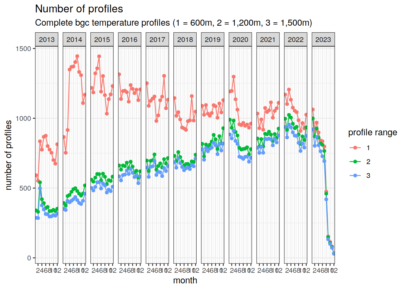
rm (bgc_temp_count, bgc_temp_count_agg)BGC - pH
bgc_ph_count <- bgc_ph %>%
  group_by(year, month, file_id, profile_range) %>%
  summarise(count_measures = n()) %>%
  ungroup()

bgc_ph_count <- bgc_ph_count %>%
  group_by(year, month, profile_range) %>%
  summarise(count_profiles = n()) %>%
  ungroup()

bgc_ph_count_agg <- bgc_ph_count %>%
  group_by(year, month) %>%
  summarise(count_profiles = sum(count_profiles)) %>%
  mutate(profile_range = 1) %>%
  ungroup()

bgc_ph_count_agg <- rbind(
  bgc_ph_count_agg,
  bgc_ph_count %>%
    filter (profile_range %in% c(2, 3)) %>%
    group_by(year, month) %>%
    summarise(count_profiles = sum(count_profiles)) %>%
    mutate(profile_range = 2) %>%
    ungroup()
)

bgc_ph_count_agg <- rbind(
  bgc_ph_count_agg,
  bgc_ph_count %>%
    filter (profile_range ==3)
)

# count of pH profiles by year, month and profile range
bgc_ph_count_agg %>%
  ggplot(aes(x = month, y = count_profiles, col = as.character(profile_range))) +
  geom_line() +
  geom_point() +
  facet_grid(. ~ year,
             scales = "free_y") +
  scale_x_continuous(breaks = seq(2,12,2)) +
  labs(x = 'month',
       y = 'number of profiles',
       col = 'profile range',
       title = "Number of profiles",
       subtitle = "Complete bgc pH profiles (1 = 614m, 2 = 1,225m, 3 = 1,600m)")
rm (bgc_ph_count, bgc_ph_count_agg)BGC - temp AND pH
bgc_ph_temp <- inner_join(bgc_ph, bgc_temp %>% distinct(file_id))

bgc_ph_temp_count <- bgc_ph_temp %>%
  group_by(year, month, file_id, profile_range) %>%
  summarise(count_measures = n()) %>%
  ungroup()

bgc_ph_temp_count <- bgc_ph_temp_count %>%
  group_by(year, month, profile_range) %>%
  summarise(count_profiles = n()) %>%
  ungroup()

bgc_ph_temp_count_agg <- bgc_ph_temp_count %>%
  group_by(year, month) %>%
  summarise(count_profiles = sum(count_profiles)) %>%
  mutate(profile_range = 1) %>%
  ungroup()

bgc_ph_temp_count_agg <- rbind(
  bgc_ph_temp_count_agg,
  bgc_ph_temp_count %>%
    filter (profile_range %in% c(2, 3)) %>%
    group_by(year, month) %>%
    summarise(count_profiles = sum(count_profiles)) %>%
    mutate(profile_range = 2) %>%
    ungroup()
)

bgc_ph_temp_count_agg <- rbind(
  bgc_ph_temp_count_agg,
  bgc_ph_temp_count %>%
    filter (profile_range ==3)
)

# count of temperature AND pH profiles by year, month and profile range
bgc_ph_temp_count_agg %>%
  ggplot(aes(x = month, y = count_profiles, col = as.character(profile_range))) +
  geom_line() +
  geom_point() +
  facet_grid(. ~ year,
             scales = "free_y") +
  scale_x_continuous(breaks = seq(2,12,2)) +
  labs(x = 'month',
       y = 'number of profiles',
       col = 'profile range',
       title = "Number of profiles",
       subtitle = "Complete bgc temperature AND pH profiles (1 = 614m, 2 = 1,225m, 3 = 1,600m)")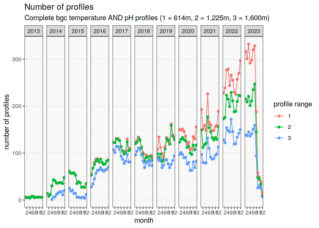
rm (bgc_ph_temp, bgc_ph_temp_count, bgc_ph_temp_count_agg)BGC - dissolved oxygen
bgc_doxy_count <- bgc_doxy %>%
  group_by(year, month, file_id, profile_range) %>%
  summarise(count_measures = n()) %>%
  ungroup()

bgc_doxy_count <- bgc_doxy_count %>%
  group_by(year, month, profile_range) %>%
  summarise(count_profiles = n()) %>%
  ungroup()

bgc_doxy_count_agg <- bgc_doxy_count %>%
  group_by(year, month) %>%
  summarise(count_profiles = sum(count_profiles)) %>%
  mutate(profile_range = 1) %>%
  ungroup()

bgc_doxy_count_agg <- rbind(
  bgc_doxy_count_agg,
  bgc_doxy_count %>%
    filter (profile_range %in% c(2, 3)) %>%
    group_by(year, month) %>%
    summarise(count_profiles = sum(count_profiles)) %>%
    mutate(profile_range = 2) %>%
    ungroup()
)

bgc_doxy_count_agg <- rbind(
  bgc_doxy_count_agg,
  bgc_doxy_count %>%
    filter (profile_range ==3)
)

# count of dissolved oxygen profiles by year, month and profile range
bgc_doxy_count_agg %>%
  ggplot(aes(x = month, y = count_profiles, col = as.character(profile_range))) +
  geom_line() +
  geom_point() +
  facet_grid(. ~ year,
             scales = "free_y") +
  scale_x_continuous(breaks = seq(2,12,2)) +
  labs(x = 'month',
       y = 'number of profiles',
       col = 'profile range',
       title = "Number of profiles",
       subtitle = "Complete bgc dissolved oxygen profiles (1 = 614m, 2 = 1,225m, 3 = 1,600m)")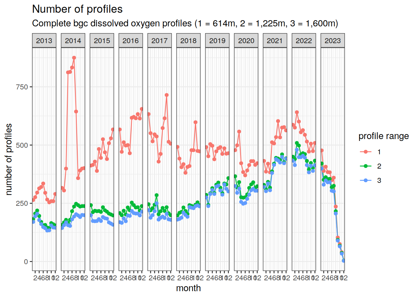
rm (bgc_doxy_count, bgc_doxy_count_agg)BGC - temp AND dissolved oxygen
bgc_doxy_temp <- inner_join(bgc_doxy, bgc_temp %>% distinct(file_id))

bgc_doxy_temp_count <- bgc_doxy_temp %>%
  group_by(year, month, file_id, profile_range) %>%
  summarise(count_measures = n()) %>%
  ungroup()

bgc_doxy_temp_count <- bgc_doxy_temp_count %>%
  group_by(year, month, profile_range) %>%
  summarise(count_profiles = n()) %>%
  ungroup()

bgc_doxy_temp_count_agg <- bgc_doxy_temp_count %>%
  group_by(year, month) %>%
  summarise(count_profiles = sum(count_profiles)) %>%
  mutate(profile_range = 1) %>%
  ungroup()

bgc_doxy_temp_count_agg <- rbind(
  bgc_doxy_temp_count_agg,
  bgc_doxy_temp_count %>%
    filter (profile_range %in% c(2, 3)) %>%
    group_by(year, month) %>%
    summarise(count_profiles = sum(count_profiles)) %>%
    mutate(profile_range = 2) %>%
    ungroup()
)

bgc_doxy_temp_count_agg <- rbind(
  bgc_doxy_temp_count_agg,
  bgc_doxy_temp_count %>%
    filter (profile_range ==3)
)

# count of temperature AND dissolved oxygen profiles by year, month and profile range
bgc_doxy_temp_count_agg %>%
  ggplot(aes(x = month, y = count_profiles, col = as.character(profile_range))) +
  geom_line() +
  geom_point() +
  facet_grid(. ~ year,
             scales = "free_y") +
  scale_x_continuous(breaks = seq(2,12,2)) +
  labs(x = 'month',
       y = 'number of profiles',
       col = 'profile range',
       title = "Number of profiles",
       subtitle = "Complete bgc temperature AND dissolved oxygen profiles (1 = 614m, 2 = 1,225m, 3 = 1,600m)")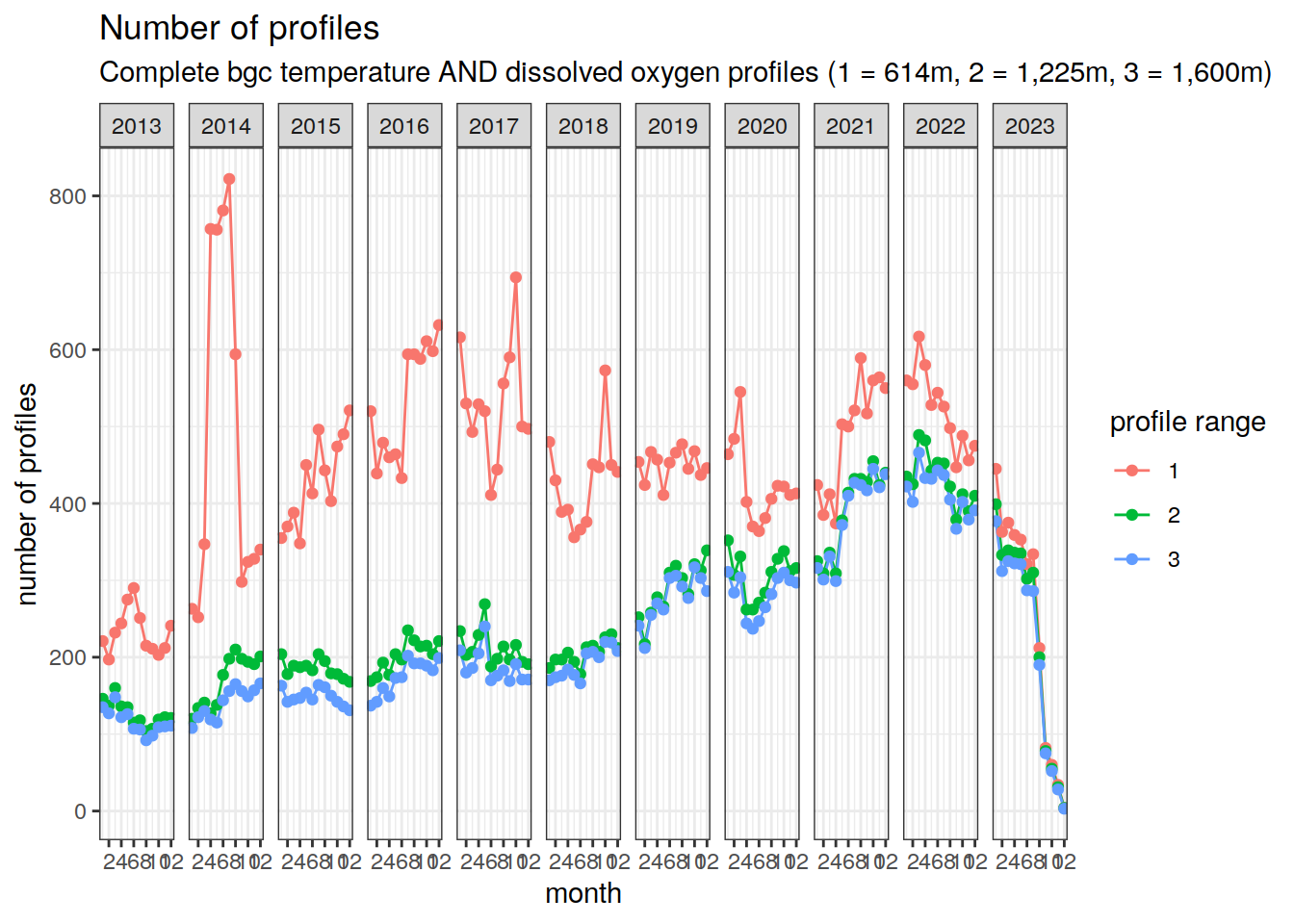
rm (bgc_doxy_temp, bgc_doxy_temp_count, bgc_doxy_temp_count_agg)BGC - nitrate
bgc_nitrate_count <- bgc_nitrate %>%
  group_by(year, month, file_id, profile_range) %>%
  summarise(count_measures = n()) %>%
  ungroup()

bgc_nitrate_count <- bgc_nitrate_count %>%
  group_by(year, month, profile_range) %>%
  summarise(count_profiles = n()) %>%
  ungroup()

bgc_nitrate_count_agg <- bgc_nitrate_count %>%
  group_by(year, month) %>%
  summarise(count_profiles = sum(count_profiles)) %>%
  mutate(profile_range = 1) %>%
  ungroup()

bgc_nitrate_count_agg <- rbind(
  bgc_nitrate_count_agg,
  bgc_nitrate_count %>%
    filter (profile_range %in% c(2, 3)) %>%
    group_by(year, month) %>%
    summarise(count_profiles = sum(count_profiles)) %>%
    mutate(profile_range = 2) %>%
    ungroup()
)

bgc_nitrate_count_agg <- rbind(
  bgc_nitrate_count_agg,
  bgc_nitrate_count %>%
    filter (profile_range ==3)
)

# count of nitrate profiles by year, month and profile range
bgc_nitrate_count_agg %>%
  ggplot(aes(x = month, y = count_profiles, col = as.character(profile_range))) +
  geom_line() +
  geom_point() +
  facet_grid(. ~ year,
             scales = "free_y") +
  scale_x_continuous(breaks = seq(2,12,2)) +
  labs(x = 'month',
       y = 'number of profiles',
       col = 'profile range',
       title = "Number of profiles",
       subtitle = "Complete bgc nitrate profiles (1 = 614m, 2 = 1,225m, 3 = 1,600m)")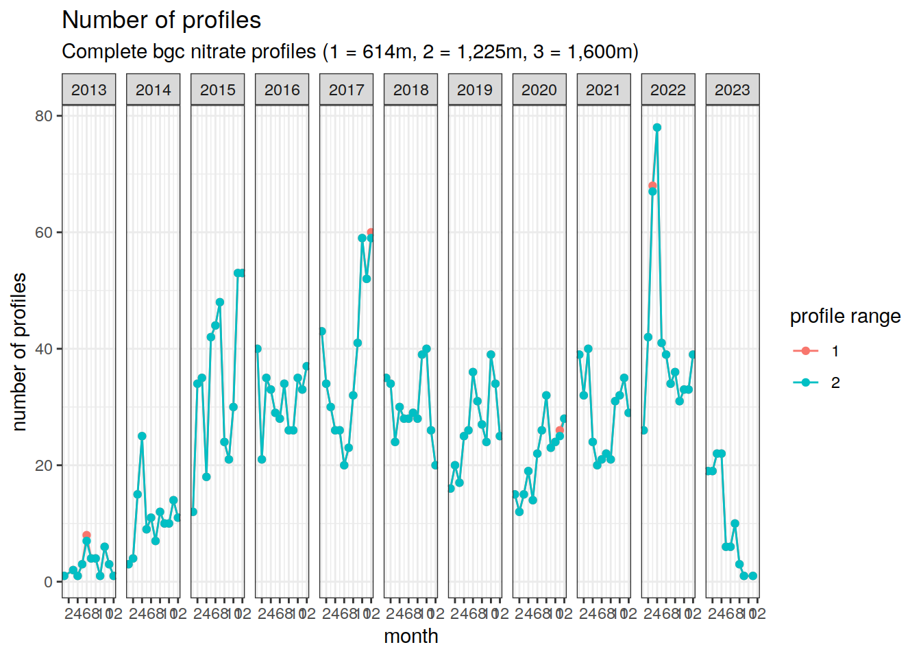
rm (bgc_nitrate_count, bgc_nitrate_count_agg)BGC - temp AND nitrate
bgc_nitrate_temp <- inner_join(bgc_nitrate, bgc_temp %>% distinct(file_id))

bgc_nitrate_temp_count <- bgc_nitrate_temp %>%
  group_by(year, month, file_id, profile_range) %>%
  summarise(count_measures = n()) %>%
  ungroup()

bgc_nitrate_temp_count <- bgc_nitrate_temp_count %>%
  group_by(year, month, profile_range) %>%
  summarise(count_profiles = n()) %>%
  ungroup()

bgc_nitrate_temp_count_agg <- bgc_nitrate_temp_count %>%
  group_by(year, month) %>%
  summarise(count_profiles = sum(count_profiles)) %>%
  mutate(profile_range = 1) %>%
  ungroup()

bgc_nitrate_temp_count_agg <- rbind(
  bgc_nitrate_temp_count_agg,
  bgc_nitrate_temp_count %>%
    filter (profile_range %in% c(2, 3)) %>%
    group_by(year, month) %>%
    summarise(count_profiles = sum(count_profiles)) %>%
    mutate(profile_range = 2) %>%
    ungroup()
)

bgc_nitrate_temp_count_agg <- rbind(
  bgc_nitrate_temp_count_agg,
  bgc_nitrate_temp_count %>%
    filter (profile_range ==3)
)

# count of temperature AND nitrate profiles by year, month and profile range
bgc_nitrate_temp_count_agg %>%
  ggplot(aes(x = month, y = count_profiles, col = as.character(profile_range))) +
  geom_line() +
  geom_point() +
  facet_grid(. ~ year,
             scales = "free_y") +
  scale_x_continuous(breaks = seq(2,12,2)) +
  labs(x = 'month',
       y = 'number of profiles',
       col = 'profile range',
       title = "Number of profiles",
       subtitle = "Complete bgc temperature AND nitrate profiles (1 = 614m, 2 = 1,225m, 3 = 1,600m)")
rm (bgc_nitrate_temp, bgc_nitrate_temp_count, bgc_nitrate_temp_count_agg)BGC - chlorophyll a
bgc_chla_count <- bgc_chla %>%
  group_by(year, month, file_id, profile_range) %>%
  summarise(count_measures = n()) %>%
  ungroup()

bgc_chla_count <- bgc_chla_count %>%
  group_by(year, month, profile_range) %>%
  summarise(count_profiles = n()) %>%
  ungroup()

bgc_chla_count_agg <- bgc_chla_count %>%
  group_by(year, month) %>%
  summarise(count_profiles = sum(count_profiles)) %>%
  mutate(profile_range = 1) %>%
  ungroup()

bgc_chla_count_agg <- rbind(
  bgc_chla_count_agg,
  bgc_chla_count %>%
    filter (profile_range %in% c(2, 3)) %>%
    group_by(year, month) %>%
    summarise(count_profiles = sum(count_profiles)) %>%
    mutate(profile_range = 2) %>%
    ungroup()
)

bgc_chla_count_agg <- rbind(
  bgc_chla_count_agg,
  bgc_chla_count %>%
    filter (profile_range ==3)
)

# count of chlorophyll a profiles by year, month and profile range
bgc_chla_count_agg %>%
  ggplot(aes(x = month, y = count_profiles, col = as.character(profile_range))) +
  geom_line() +
  geom_point() +
  facet_grid(. ~ year,
             scales = "free_y") +
  scale_x_continuous(breaks = seq(2,12,2)) +
  labs(x = 'month',
       y = 'number of profiles',
       col = 'profile range',
       title = "Number of profiles",
       subtitle = "Complete bgc chlorophyll a profiles (1 = 614m, 2 = 1,225m, 3 = 1,600m)")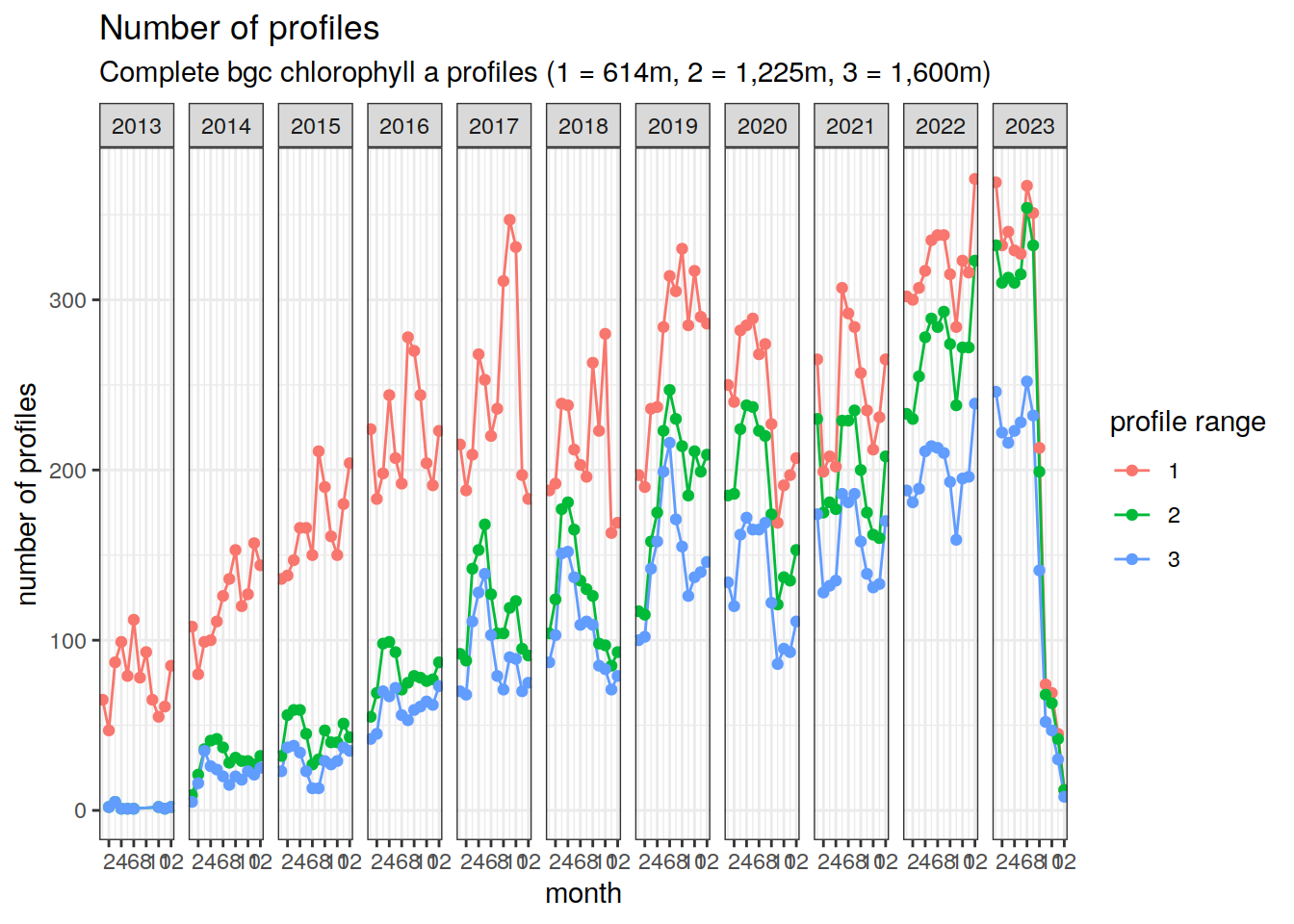
rm (bgc_chla_count, bgc_chla_count_agg)BGC - temp AND chlorophyll a
bgc_chla_temp <- inner_join(bgc_chla, bgc_temp %>% distinct(file_id))

bgc_chla_temp_count <- bgc_chla_temp %>%
  group_by(year, month, file_id, profile_range) %>%
  summarise(count_measures = n()) %>%
  ungroup()

bgc_chla_temp_count <- bgc_chla_temp_count %>%
  group_by(year, month, profile_range) %>%
  summarise(count_profiles = n()) %>%
  ungroup()

bgc_chla_temp_count_agg <- bgc_chla_temp_count %>%
  group_by(year, month) %>%
  summarise(count_profiles = sum(count_profiles)) %>%
  mutate(profile_range = 1) %>%
  ungroup()

bgc_chla_temp_count_agg <- rbind(
  bgc_chla_temp_count_agg,
  bgc_chla_temp_count %>%
    filter (profile_range %in% c(2, 3)) %>%
    group_by(year, month) %>%
    summarise(count_profiles = sum(count_profiles)) %>%
    mutate(profile_range = 2) %>%
    ungroup()
)

bgc_chla_temp_count_agg <- rbind(
  bgc_chla_temp_count_agg,
  bgc_chla_temp_count %>%
    filter (profile_range ==3)
)

# count of temperature AND chlorophyll a profiles by year, month and profile range
bgc_chla_temp_count_agg %>%
  ggplot(aes(x = month, y = count_profiles, col = as.character(profile_range))) +
  geom_line() +
  geom_point() +
  facet_grid(. ~ year,
             scales = "free_y") +
  scale_x_continuous(breaks = seq(2,12,2)) +
  labs(x = 'month',
       y = 'number of profiles',
       col = 'profile range',
       title = "Number of profiles",
       subtitle = "Complete bgc temperature AND chlorophyll a profiles (1 = 614m, 2 = 1,225m, 3 = 1,600m)")
rm (bgc_chla_temp, bgc_chla_temp_count, bgc_chla_temp_count_agg)BGC - temp, pH, doxy, nitrate AND chl a
bgc_all <- inner_join(bgc_ph, bgc_temp %>% distinct(file_id))
bgc_all <- inner_join(bgc_all, bgc_doxy %>% distinct(file_id))
bgc_all <- inner_join(bgc_all, bgc_nitrate %>% distinct(file_id))
bgc_all <- inner_join(bgc_all, bgc_chla %>% distinct(file_id))

bgc_all_count <- bgc_all %>%
  group_by(year, month, file_id, profile_range) %>%
  summarise(count_measures = n()) %>%
  ungroup()

bgc_all_count <- bgc_all_count %>%
  group_by(year, month, profile_range) %>%
  summarise(count_profiles = n()) %>%
  ungroup()

bgc_all_count_agg <- bgc_all_count %>%
  group_by(year, month) %>%
  summarise(count_profiles = sum(count_profiles)) %>%
  mutate(profile_range = 1) %>%
  ungroup()

bgc_all_count_agg <- rbind(
  bgc_all_count_agg,
  bgc_all_count %>%
    filter (profile_range %in% c(2, 3)) %>%
    group_by(year, month) %>%
    summarise(count_profiles = sum(count_profiles)) %>%
    mutate(profile_range = 2) %>%
    ungroup()
)

bgc_all_count_agg <- rbind(
  bgc_all_count_agg,
  bgc_all_count %>%
    filter (profile_range ==3)
)

# count of temp, pH, doxy, nitrate AND chl a profiles by year, month and profile range
bgc_all_count_agg %>%
  ggplot(aes(x = month, y = count_profiles, col = as.character(profile_range))) +
  geom_line() +
  geom_point() +
  facet_grid(. ~ year,
             scales = "free_y") +
  scale_x_continuous(breaks = seq(2,12,2)) +
  labs(x = 'month',
       y = 'number of profiles',
       col = 'profile range',
       title = "Number of profiles",
       subtitle = "Complete bgc temp, pH, doxy, nitrate AND chl a profiles (1 = 614m, 2 = 1,225m, 3 = 1,600m)")
rm (bgc_all, bgc_all_count, bgc_all_count_agg)
sessionInfo()R version 4.2.2 (2022-10-31)
Platform: x86_64-pc-linux-gnu (64-bit)
Running under: openSUSE Leap 15.5
Matrix products: default
BLAS: /usr/local/R-4.2.2/lib64/R/lib/libRblas.so
LAPACK: /usr/local/R-4.2.2/lib64/R/lib/libRlapack.so
locale:
[1] LC_CTYPE=en_US.UTF-8 LC_NUMERIC=C
[3] LC_TIME=en_US.UTF-8 LC_COLLATE=en_US.UTF-8
[5] LC_MONETARY=en_US.UTF-8 LC_MESSAGES=en_US.UTF-8
[7] LC_PAPER=en_US.UTF-8 LC_NAME=C
[9] LC_ADDRESS=C LC_TELEPHONE=C
[11] LC_MEASUREMENT=en_US.UTF-8 LC_IDENTIFICATION=C
attached base packages:
[1] stats graphics grDevices utils datasets methods base
other attached packages:
[1] lubridate_1.9.0 timechange_0.1.1 argodata_0.1.0 forcats_0.5.2
[5] stringr_1.5.0 dplyr_1.1.3 purrr_1.0.2 readr_2.1.3
[9] tidyr_1.3.0 tibble_3.2.1 ggplot2_3.4.4 tidyverse_1.3.2
[13] workflowr_1.7.0
loaded via a namespace (and not attached):
[1] Rcpp_1.0.10 getPass_0.2-2 ps_1.7.2
[4] assertthat_0.2.1 rprojroot_2.0.3 digest_0.6.30
[7] utf8_1.2.2 R6_2.5.1 cellranger_1.1.0
[10] backports_1.4.1 reprex_2.0.2 evaluate_0.18
[13] highr_0.9 httr_1.4.4 pillar_1.9.0
[16] rlang_1.1.1 readxl_1.4.1 googlesheets4_1.0.1
[19] rstudioapi_0.15.0 whisker_0.4 callr_3.7.3
[22] jquerylib_0.1.4 rmarkdown_2.18 labeling_0.4.2
[25] googledrive_2.0.0 munsell_0.5.0 broom_1.0.5
[28] compiler_4.2.2 httpuv_1.6.6 modelr_0.1.10
[31] xfun_0.35 pkgconfig_2.0.3 htmltools_0.5.3
[34] tidyselect_1.2.0 fansi_1.0.3 crayon_1.5.2
[37] withr_2.5.0 tzdb_0.3.0 dbplyr_2.2.1
[40] later_1.3.0 grid_4.2.2 jsonlite_1.8.3
[43] gtable_0.3.1 lifecycle_1.0.3 DBI_1.1.3
[46] git2r_0.30.1 magrittr_2.0.3 scales_1.2.1
[49] cli_3.6.1 stringi_1.7.8 cachem_1.0.6
[52] farver_2.1.1 fs_1.5.2 promises_1.2.0.1
[55] xml2_1.3.3 bslib_0.4.1 ellipsis_0.3.2
[58] generics_0.1.3 vctrs_0.6.4 tools_4.2.2
[61] glue_1.6.2 RNetCDF_2.6-1 hms_1.1.2
[64] processx_3.8.0 fastmap_1.1.0 yaml_2.3.6
[67] colorspace_2.0-3 gargle_1.2.1 rvest_1.0.3
[70] knitr_1.41 haven_2.5.1 sass_0.4.4