Results publication
Jens Daniel Müller
17 January, 2023
Last updated: 2023-01-17
Checks: 7 0
Knit directory:
emlr_obs_analysis/analysis/
This reproducible R Markdown analysis was created with workflowr (version 1.7.0). The Checks tab describes the reproducibility checks that were applied when the results were created. The Past versions tab lists the development history.
Great! Since the R Markdown file has been committed to the Git repository, you know the exact version of the code that produced these results.
Great job! The global environment was empty. Objects defined in the global environment can affect the analysis in your R Markdown file in unknown ways. For reproduciblity it’s best to always run the code in an empty environment.
The command set.seed(20210412) was run prior to running
the code in the R Markdown file. Setting a seed ensures that any results
that rely on randomness, e.g. subsampling or permutations, are
reproducible.
Great job! Recording the operating system, R version, and package versions is critical for reproducibility.
Nice! There were no cached chunks for this analysis, so you can be confident that you successfully produced the results during this run.
Great job! Using relative paths to the files within your workflowr project makes it easier to run your code on other machines.
Great! You are using Git for version control. Tracking code development and connecting the code version to the results is critical for reproducibility.
The results in this page were generated with repository version 30b15de. See the Past versions tab to see a history of the changes made to the R Markdown and HTML files.
Note that you need to be careful to ensure that all relevant files for
the analysis have been committed to Git prior to generating the results
(you can use wflow_publish or
wflow_git_commit). workflowr only checks the R Markdown
file, but you know if there are other scripts or data files that it
depends on. Below is the status of the Git repository when the results
were generated:
Ignored files:
    Ignored:    .Rhistory
    Ignored:    .Rproj.user/
    Ignored:    data/
    Ignored:    output/other/
    Ignored:    output/presentation/
    Ignored:    output/publication/

Untracked files:
    Untracked:  code/RScript_Jens_globalMap.R
    Untracked:  code/choky-barb_reprex.R
    Untracked:  code/choky-barb_reprex.md
    Untracked:  code/choky-barb_reprex_files/
    Untracked:  code/raster_dataframe.R
    Untracked:  code/results_publication_backup_incl_ensemble_uncertainty_20221111.Rmd
    Untracked:  code/tidyterra_spatRaster.R
    Untracked:  code/write_ocean_raster_netcdf.R
    Untracked:  ok-coqui_reprex_files/

Unstaged changes:
    Modified:   analysis/G19_column_inventories.Rmd
    Deleted:    analysis/MLR_target_budgets.Rmd
    Deleted:    analysis/MLR_target_column_inventories.Rmd
    Deleted:    analysis/MLR_target_zonal_sections.Rmd
    Modified:   analysis/_site.yml
    Modified:   analysis/basics.Rmd
    Modified:   code/Workflowr_project_managment.R
Note that any generated files, e.g. HTML, png, CSS, etc., are not included in this status report because it is ok for generated content to have uncommitted changes.
These are the previous versions of the repository in which changes were
made to the R Markdown (analysis/results_publication.Rmd)
and HTML (docs/results_publication.html) files. If you’ve
configured a remote Git repository (see ?wflow_git_remote),
click on the hyperlinks in the table below to view the files as they
were in that past version.
| File | Version | Author | Date | Message |
|---|---|---|---|---|
| Rmd | 30b15de | jens-daniel-mueller | 2023-01-17 | changed label |
| html | fdf5f22 | jens-daniel-mueller | 2023-01-11 | Build site. |
| Rmd | 657f205 | jens-daniel-mueller | 2023-01-11 | revised plots for talk |
| html | 2cca4eb | jens-daniel-mueller | 2023-01-10 | Build site. |
| Rmd | 532c24a | jens-daniel-mueller | 2023-01-10 | revised plots |
| html | 8ded995 | jens-daniel-mueller | 2023-01-05 | Build site. |
| Rmd | 80fac85 | jens-daniel-mueller | 2023-01-05 | converted all maps to robinson projection |
| html | b9d5a73 | jens-daniel-mueller | 2022-12-15 | Build site. |
| Rmd | fe0def4 | jens-daniel-mueller | 2022-12-15 | included robinson raster maps |
| html | 0f2c9d5 | jens-daniel-mueller | 2022-12-08 | Build site. |
| Rmd | ee5cdab | jens-daniel-mueller | 2022-12-08 | minor figure updates |
| html | 445761e | jens-daniel-mueller | 2022-12-02 | Build site. |
| Rmd | ab1269e | jens-daniel-mueller | 2022-12-02 | GCB budget tables compiled |
| html | ef50aa6 | jens-daniel-mueller | 2022-11-30 | Build site. |
| Rmd | 104a756 | jens-daniel-mueller | 2022-11-29 | refined BIM color scale |
| html | 439cb85 | jens-daniel-mueller | 2022-11-29 | Build site. |
| Rmd | c01f61e | jens-daniel-mueller | 2022-11-29 | refined BIM estimates |
| html | 9048dc4 | jens-daniel-mueller | 2022-11-29 | Build site. |
| Rmd | 533e469 | jens-daniel-mueller | 2022-11-29 | included BIM estimates |
| html | 3a7bab0 | jens-daniel-mueller | 2022-11-28 | Build site. |
| Rmd | 5f54639 | jens-daniel-mueller | 2022-11-28 | minor figure revisions |
| html | 322b1c1 | jens-daniel-mueller | 2022-11-25 | Build site. |
| Rmd | 0447054 | jens-daniel-mueller | 2022-11-25 | 1 and 2 sigma uncertainty |
| html | 491f8b1 | jens-daniel-mueller | 2022-11-25 | Build site. |
| Rmd | 6a7dfb4 | jens-daniel-mueller | 2022-11-25 | 2 sigma uncertainty |
| html | 4da4d66 | jens-daniel-mueller | 2022-11-25 | Build site. |
| Rmd | 18f0c96 | jens-daniel-mueller | 2022-11-25 | 1 sigma uncertainty |
| html | 534ee74 | jens-daniel-mueller | 2022-11-25 | Build site. |
| Rmd | d682344 | jens-daniel-mueller | 2022-11-24 | tested OceanSODA surface dcant based on regression trend |
| Rmd | 9e119d5 | jens-daniel-mueller | 2022-11-23 | revised penetration depth estimates, adapted new uncertainty estimates throughout |
| html | 57d1a9b | jens-daniel-mueller | 2022-11-17 | Build site. |
| Rmd | a56474c | jens-daniel-mueller | 2022-11-17 | new emissions uncertainty |
| html | f39bfd4 | jens-daniel-mueller | 2022-11-17 | Build site. |
| Rmd | 71e9efe | jens-daniel-mueller | 2022-11-17 | converted scaling uncertainty contribution to 1 sigma |
| html | e924c80 | jens-daniel-mueller | 2022-11-17 | Build site. |
| Rmd | cc118f6 | jens-daniel-mueller | 2022-11-17 | revised additive uncertainty calculation |
| html | 8e1702d | jens-daniel-mueller | 2022-11-16 | Build site. |
| Rmd | 5cf1489 | jens-daniel-mueller | 2022-11-16 | revised inventory uncertainty calculation |
| html | ea34027 | jens-daniel-mueller | 2022-11-15 | Build site. |
| Rmd | be95f92 | jens-daniel-mueller | 2022-11-15 | exported residual correlation plot |
| html | 8ac0da0 | jens-daniel-mueller | 2022-11-15 | Build site. |
| Rmd | 63fb2fb | jens-daniel-mueller | 2022-11-15 | more units expressed per decade |
| html | 5520de8 | jens-daniel-mueller | 2022-11-15 | Build site. |
| Rmd | 751a519 | jens-daniel-mueller | 2022-11-15 | units expressed per decade |
| html | 1dad51a | jens-daniel-mueller | 2022-11-15 | Build site. |
| Rmd | ab89db3 | jens-daniel-mueller | 2022-11-15 | surface emlr extrapolated without surface obs |
| html | 375300e | jens-daniel-mueller | 2022-11-14 | Build site. |
| Rmd | 40f357d | jens-daniel-mueller | 2022-11-14 | included C* and DIC target cases |
| html | ebc85e2 | jens-daniel-mueller | 2022-11-14 | Build site. |
| Rmd | beb709c | jens-daniel-mueller | 2022-11-14 | included C* and DIC target cases |
| html | cc337dd | jens-daniel-mueller | 2022-11-11 | Build site. |
| Rmd | c53fea0 | jens-daniel-mueller | 2022-11-11 | rebuild website with woa18 clim |
| html | 6edad9b | jens-daniel-mueller | 2022-11-11 | Build site. |
| Rmd | 9937e55 | jens-daniel-mueller | 2022-11-11 | with additive uncertainty estimates |
| html | 16beb51 | jens-daniel-mueller | 2022-11-08 | Build site. |
| Rmd | 6276ead | jens-daniel-mueller | 2022-11-08 | run with all contribution, but exclude AT and reoccupation in inventories |
| html | b92657d | jens-daniel-mueller | 2022-11-08 | Build site. |
| Rmd | 3f9fad2 | jens-daniel-mueller | 2022-11-08 | run without C*(P only) and SD factor 2 |
| html | 0b939ca | jens-daniel-mueller | 2022-11-08 | Build site. |
| Rmd | 5c705d7 | jens-daniel-mueller | 2022-11-08 | run with C*(P only) |
| html | ec60f68 | jens-daniel-mueller | 2022-11-07 | Build site. |
| html | 7275091 | jens-daniel-mueller | 2022-11-05 | Build site. |
| Rmd | ba55b15 | jens-daniel-mueller | 2022-11-05 | include run with C*(P only) |
| html | 99610ed | jens-daniel-mueller | 2022-11-01 | Build site. |
| Rmd | c972beb | jens-daniel-mueller | 2022-11-01 | updated reoccupation run |
| html | 7060801 | jens-daniel-mueller | 2022-10-31 | Build site. |
| html | ecb84c1 | jens-daniel-mueller | 2022-10-30 | Build site. |
| html | 2345935 | jens-daniel-mueller | 2022-10-29 | Build site. |
| html | 0b40366 | jens-daniel-mueller | 2022-10-26 | Build site. |
| Rmd | 0465788 | jens-daniel-mueller | 2022-10-26 | implemented additive uncertainty assesment |
| html | 91052ae | jens-daniel-mueller | 2022-10-20 | Build site. |
| Rmd | 33486a1 | jens-daniel-mueller | 2022-10-20 | updated plots |
| html | 084a41c | jens-daniel-mueller | 2022-10-13 | Build site. |
| Rmd | ffef558 | jens-daniel-mueller | 2022-10-13 | land sink assesment |
| html | 46c163a | jens-daniel-mueller | 2022-10-10 | Build site. |
| Rmd | 78161f9 | jens-daniel-mueller | 2022-10-10 | revised figures |
| html | 8105380 | jens-daniel-mueller | 2022-10-07 | Build site. |
| Rmd | d663118 | jens-daniel-mueller | 2022-10-07 | penetration depth analysis |
| html | e93fdfd | jens-daniel-mueller | 2022-09-23 | Build site. |
| Rmd | f01db23 | jens-daniel-mueller | 2022-09-23 | added uncertainty to dcant maps and section |
| html | 8dc5a3b | jens-daniel-mueller | 2022-09-09 | Build site. |
| Rmd | 25bff3d | jens-daniel-mueller | 2022-09-09 | added global section location to maps |
| html | 77e6a80 | jens-daniel-mueller | 2022-09-08 | Build site. |
| Rmd | 188dc63 | jens-daniel-mueller | 2022-09-08 | added uncertainty to global section |
| html | 7cf954e | jens-daniel-mueller | 2022-09-08 | Build site. |
| Rmd | 6f53c28 | jens-daniel-mueller | 2022-09-08 | column inventory uncertainty stippling added |
| html | 051b911 | jens-daniel-mueller | 2022-09-07 | Build site. |
| Rmd | c87415f | jens-daniel-mueller | 2022-09-07 | testrun integration 3000 |
| html | 75bd58c | jens-daniel-mueller | 2022-09-07 | Build site. |
| Rmd | 1024099 | jens-daniel-mueller | 2022-09-07 | testrun integration 1000 |
| html | 1c6de0d | jens-daniel-mueller | 2022-09-07 | Build site. |
| Rmd | 4106aa4 | jens-daniel-mueller | 2022-09-07 | testrun integration 10000 |
| html | 5ca8778 | jens-daniel-mueller | 2022-09-07 | Build site. |
| Rmd | 784849d | jens-daniel-mueller | 2022-09-07 | included uncertainty assesment for column inventories |
| html | 4eb9ed2 | jens-daniel-mueller | 2022-08-29 | Build site. |
| html | 392f3d7 | jens-daniel-mueller | 2022-08-29 | Build site. |
| Rmd | 282421f | jens-daniel-mueller | 2022-08-29 | added contour line to global section |
| html | c975141 | jens-daniel-mueller | 2022-08-29 | Build site. |
| Rmd | 8f5c3c2 | jens-daniel-mueller | 2022-08-29 | finalized global section |
| html | cf69673 | jens-daniel-mueller | 2022-08-29 | Build site. |
| html | 4810db6 | jens-daniel-mueller | 2022-08-26 | Build site. |
| Rmd | 88ce2d9 | jens-daniel-mueller | 2022-08-26 | added global section |
| html | 74dca9d | jens-daniel-mueller | 2022-08-17 | Build site. |
| Rmd | 37ab61f | jens-daniel-mueller | 2022-08-17 | added adjustment delta map |
| html | ec4f1d0 | jens-daniel-mueller | 2022-08-11 | Build site. |
| Rmd | d1cd39a | jens-daniel-mueller | 2022-08-11 | revised figure aspect ratio |
| html | 78dbb27 | jens-daniel-mueller | 2022-08-11 | Build site. |
| Rmd | 2155209 | jens-daniel-mueller | 2022-08-11 | rebuild with 3 basin separation as standard case |
| html | 302d289 | jens-daniel-mueller | 2022-08-11 | Build site. |
| Rmd | 77719db | jens-daniel-mueller | 2022-08-11 | rebuild with 5 basin separation as standard case |
| html | 318fefe | jens-daniel-mueller | 2022-08-11 | Build site. |
| Rmd | 60dae4b | jens-daniel-mueller | 2022-08-11 | delta dcant budget analysis |
| html | 5b77c4f | jens-daniel-mueller | 2022-08-10 | Build site. |
| Rmd | c25333a | jens-daniel-mueller | 2022-08-10 | bias sections and maps added |
| html | 9c3be27 | jens-daniel-mueller | 2022-08-09 | Build site. |
| Rmd | a940880 | jens-daniel-mueller | 2022-08-09 | improve delta dcant bias assesment |
| html | a691b29 | jens-daniel-mueller | 2022-08-09 | Build site. |
| Rmd | d136a86 | jens-daniel-mueller | 2022-08-09 | include delta dcant bias assesment |
| html | 910f96e | jens-daniel-mueller | 2022-08-08 | Build site. |
| Rmd | e064958 | jens-daniel-mueller | 2022-08-08 | include bias assesment |
| html | e99640e | jens-daniel-mueller | 2022-07-29 | Build site. |
| html | f68fcfa | jens-daniel-mueller | 2022-07-26 | Build site. |
| Rmd | abec0de | jens-daniel-mueller | 2022-07-26 | changed color scale back |
| html | f2615fb | jens-daniel-mueller | 2022-07-26 | Build site. |
| Rmd | 8da318e | jens-daniel-mueller | 2022-07-26 | changed color scale |
| html | 99a82db | jens-daniel-mueller | 2022-07-25 | Build site. |
| Rmd | 1d6985d | jens-daniel-mueller | 2022-07-25 | stat analysis of layer budgets and CIs |
| html | 4af29f9 | jens-daniel-mueller | 2022-07-24 | Build site. |
| Rmd | b2c4ff6 | jens-daniel-mueller | 2022-07-24 | revised GCB plot |
| html | e2adac6 | jens-daniel-mueller | 2022-07-22 | Build site. |
| Rmd | a9c8af4 | jens-daniel-mueller | 2022-07-22 | revised section plots and tables |
| html | 9bbc6a4 | jens-daniel-mueller | 2022-07-20 | Build site. |
| Rmd | f937de2 | jens-daniel-mueller | 2022-07-20 | revised plots |
| html | 0c6db30 | jens-daniel-mueller | 2022-07-20 | Build site. |
| Rmd | a42e52d | jens-daniel-mueller | 2022-07-20 | revised plots |
| html | b18b250 | jens-daniel-mueller | 2022-07-20 | Build site. |
| Rmd | 36691bf | jens-daniel-mueller | 2022-07-20 | revised plots |
| html | a80b59b | jens-daniel-mueller | 2022-07-20 | Build site. |
| Rmd | f9c0545 | jens-daniel-mueller | 2022-07-20 | revised budget stats |
| html | fea41c1 | jens-daniel-mueller | 2022-07-20 | Build site. |
| Rmd | b27e42f | jens-daniel-mueller | 2022-07-20 | rerun with corrected Canyon-B talk gap-filling in standard case |
| html | 9ce772d | jens-daniel-mueller | 2022-07-19 | Build site. |
| Rmd | aaf37cf | jens-daniel-mueller | 2022-07-19 | coverage maps with gap filling |
| html | d803308 | jens-daniel-mueller | 2022-07-19 | Build site. |
| Rmd | 933285c | jens-daniel-mueller | 2022-07-19 | revised plots |
| html | b1f7ab3 | jens-daniel-mueller | 2022-07-18 | Build site. |
| Rmd | ab5220b | jens-daniel-mueller | 2022-07-18 | revised budget over atm pCO2 plot |
| html | d2ae54c | jens-daniel-mueller | 2022-07-18 | Build site. |
| Rmd | 85f482c | jens-daniel-mueller | 2022-07-18 | include scaled Sabine data for budgets |
| html | 2695085 | jens-daniel-mueller | 2022-07-17 | Build site. |
| Rmd | 8624c93 | jens-daniel-mueller | 2022-07-17 | use global output from MLR basins |
| html | 535196a | jens-daniel-mueller | 2022-07-17 | Build site. |
| html | d20faeb | jens-daniel-mueller | 2022-07-17 | Build site. |
| Rmd | b6ef86b | jens-daniel-mueller | 2022-07-17 | revised budget plots |
| html | 0160c40 | jens-daniel-mueller | 2022-07-16 | Build site. |
| Rmd | d2b1090 | jens-daniel-mueller | 2022-07-16 | cleaned code |
| html | efa414b | jens-daniel-mueller | 2022-07-16 | Build site. |
| Rmd | e84b169 | jens-daniel-mueller | 2022-07-16 | added bias global analysis |
| html | 7267b08 | jens-daniel-mueller | 2022-07-16 | Build site. |
| Rmd | b91f619 | jens-daniel-mueller | 2022-07-16 | analysed dcant budget stats |
| html | 08c00b4 | jens-daniel-mueller | 2022-07-16 | Build site. |
| html | 692c937 | jens-daniel-mueller | 2022-07-16 | Build site. |
| html | afb27ad | jens-daniel-mueller | 2022-07-15 | Build site. |
| Rmd | 53e63d5 | jens-daniel-mueller | 2022-07-15 | plot no surface data equi |
| html | b492b46 | jens-daniel-mueller | 2022-07-15 | Build site. |
| Rmd | 31f29fe | jens-daniel-mueller | 2022-07-15 | plot decadal sink trends as boxplots |
| html | bd24a0f | jens-daniel-mueller | 2022-07-15 | Build site. |
| Rmd | efbb1dc | jens-daniel-mueller | 2022-07-15 | include no surface equi cases |
| html | 022fd60 | jens-daniel-mueller | 2022-07-14 | Build site. |
| Rmd | 5a9e419 | jens-daniel-mueller | 2022-07-14 | implemented beta budget analysis |
| Rmd | d2092c1 | jens-daniel-mueller | 2022-07-14 | implemented beta budget analysis |
| html | f1d7f80 | jens-daniel-mueller | 2022-07-13 | Build site. |
| Rmd | 6811ae4 | jens-daniel-mueller | 2022-07-13 | refined profil plots |
| html | ea46812 | jens-daniel-mueller | 2022-07-13 | Build site. |
| Rmd | defdcfe | jens-daniel-mueller | 2022-07-13 | additional analyis |
| html | 17cd1d1 | jens-daniel-mueller | 2022-07-13 | Build site. |
| Rmd | 1bf1708 | jens-daniel-mueller | 2022-07-13 | rerun reoccupation |
| html | 26e9496 | jens-daniel-mueller | 2022-07-12 | Build site. |
| Rmd | 5d121f0 | jens-daniel-mueller | 2022-07-12 | applied dcant scaling and improved ensemble member analysis |
| html | 8fb595c | jens-daniel-mueller | 2022-07-12 | Build site. |
| Rmd | e2d97ef | jens-daniel-mueller | 2022-07-12 | excluded no adjustment from ensemble |
| html | 003b161 | jens-daniel-mueller | 2022-07-12 | Build site. |
| Rmd | 54a0d14 | jens-daniel-mueller | 2022-07-12 | added cruise based adjustment |
| html | b44c72a | jens-daniel-mueller | 2022-07-03 | Build site. |
| html | 37f56b3 | jens-daniel-mueller | 2022-07-01 | Build site. |
| Rmd | 8c4a9f8 | jens-daniel-mueller | 2022-07-01 | added basin separation analysis |
| html | 232909e | jens-daniel-mueller | 2022-07-01 | Build site. |
| Rmd | 7f85db3 | jens-daniel-mueller | 2022-07-01 | added basin separation analysis |
| html | df21d31 | jens-daniel-mueller | 2022-07-01 | Build site. |
| Rmd | 2bbfba0 | jens-daniel-mueller | 2022-07-01 | rebuild |
| html | 6be73e0 | jens-daniel-mueller | 2022-06-30 | Build site. |
| Rmd | 6e173bf | jens-daniel-mueller | 2022-06-30 | updated regional budget plots |
| html | 6e173bf | jens-daniel-mueller | 2022-06-30 | updated regional budget plots |
| html | 8ab4a87 | jens-daniel-mueller | 2022-06-29 | Build site. |
| Rmd | d8c7cb9 | jens-daniel-mueller | 2022-06-29 | ensemble with unadjusted data |
| html | 7629c78 | jens-daniel-mueller | 2022-06-29 | Build site. |
| Rmd | 4758911 | jens-daniel-mueller | 2022-06-29 | ensemble without unadjusted data |
| html | f6786c8 | jens-daniel-mueller | 2022-06-29 | Build site. |
| Rmd | 6f694a1 | jens-daniel-mueller | 2022-06-29 | included Cstar N in ensemble |
| html | f09080e | jens-daniel-mueller | 2022-06-28 | Build site. |
| Rmd | d457610 | jens-daniel-mueller | 2022-06-28 | save figures for publication |
| html | ee30748 | jens-daniel-mueller | 2022-06-28 | Build site. |
| Rmd | fe42644 | jens-daniel-mueller | 2022-06-28 | GCB emissions ratio included |
| html | 9393c07 | jens-daniel-mueller | 2022-06-28 | Build site. |
| Rmd | 2a3cf97 | jens-daniel-mueller | 2022-06-28 | included basin-hemisphere bias, and bias contributions |
| html | 0825298 | jens-daniel-mueller | 2022-06-28 | Build site. |
| Rmd | d35ddb1 | jens-daniel-mueller | 2022-06-28 | included GCB ocean sink data as boxplot |
| html | a13a7cf | jens-daniel-mueller | 2022-06-28 | Build site. |
| html | fb59a6f | jens-daniel-mueller | 2022-06-27 | Build site. |
| Rmd | 7ff568c | jens-daniel-mueller | 2022-06-27 | included GCB ocean sink data |
| html | a26a21d | jens-daniel-mueller | 2022-06-27 | Build site. |
| Rmd | 9425709 | jens-daniel-mueller | 2022-06-27 | scaled sabine 2004 to full area |
| html | 748aa43 | jens-daniel-mueller | 2022-06-27 | Build site. |
| Rmd | 82d5793 | jens-daniel-mueller | 2022-06-27 | ensemble scatter plot |
| html | 457e640 | jens-daniel-mueller | 2022-06-27 | Build site. |
| Rmd | 426c5bf | jens-daniel-mueller | 2022-06-27 | cleaned read-in section |
| html | 16dc3af | jens-daniel-mueller | 2022-06-27 | Build site. |
| Rmd | dd2063a | jens-daniel-mueller | 2022-06-27 | ensemble member analysis added |
| html | 87e9eb8 | jens-daniel-mueller | 2022-06-27 | Build site. |
| Rmd | 09a3348 | jens-daniel-mueller | 2022-06-27 | 1 as standard case and new ensemble members |
| html | b52b159 | jens-daniel-mueller | 2022-06-27 | Build site. |
| html | 09b0780 | jens-daniel-mueller | 2022-05-24 | Build site. |
| html | 25da2fb | jens-daniel-mueller | 2022-05-24 | Build site. |
| html | 1d73ec9 | jens-daniel-mueller | 2022-05-16 | Build site. |
| Rmd | e117b7b | jens-daniel-mueller | 2022-05-16 | rerun w/o data adjustments |
| html | 2ffbdda | jens-daniel-mueller | 2022-05-16 | Build site. |
| Rmd | 6fc8438 | jens-daniel-mueller | 2022-05-16 | plot individual zonal sections |
| html | c71227f | jens-daniel-mueller | 2022-05-16 | Build site. |
| Rmd | 55e9ac6 | jens-daniel-mueller | 2022-05-16 | plot individual zonal sections |
| html | 3c1100c | jens-daniel-mueller | 2022-05-16 | Build site. |
| Rmd | fdb111d | jens-daniel-mueller | 2022-05-16 | plot individual zonal sections |
| html | 2ca0109 | jens-daniel-mueller | 2022-05-02 | Build site. |
| Rmd | 63d51bd | jens-daniel-mueller | 2022-05-02 | rerun with adjusted data |
| html | dcf2eaf | jens-daniel-mueller | 2022-05-02 | Build site. |
| Rmd | a3a2cf9 | jens-daniel-mueller | 2022-05-02 | IO sections seperate |
| html | eff4fd7 | jens-daniel-mueller | 2022-05-02 | Build site. |
| Rmd | 39e920a | jens-daniel-mueller | 2022-05-02 | IO sections seperate |
| html | 08607eb | jens-daniel-mueller | 2022-05-02 | Build site. |
| Rmd | 0791c1b | jens-daniel-mueller | 2022-05-02 | modified plots |
| html | b018a9a | jens-daniel-mueller | 2022-04-29 | Build site. |
| Rmd | 02ede93 | jens-daniel-mueller | 2022-04-29 | standard case uncorrected data |
| html | e09320d | jens-daniel-mueller | 2022-04-12 | Build site. |
| Rmd | 0dec180 | jens-daniel-mueller | 2022-04-12 | 3 data adjustment procedures implemented |
| html | 8dca96a | jens-daniel-mueller | 2022-04-12 | Build site. |
| Rmd | e5e9288 | jens-daniel-mueller | 2022-04-12 | 3 data adjustment procedures implemented |
| html | 2f20ea6 | jens-daniel-mueller | 2022-04-11 | Build site. |
| html | 209c9b6 | jens-daniel-mueller | 2022-04-10 | Build site. |
| Rmd | 537aff7 | jens-daniel-mueller | 2022-04-10 | no data adjustment implemented |
| html | acad2e2 | jens-daniel-mueller | 2022-04-09 | Build site. |
| html | 3d81135 | jens-daniel-mueller | 2022-04-07 | Build site. |
| html | 0f5d372 | jens-daniel-mueller | 2022-04-04 | Build site. |
| Rmd | ac5121f | jens-daniel-mueller | 2022-04-04 | added zonal mean beta distribution new figure |
| html | 1b5a309 | jens-daniel-mueller | 2022-04-04 | Build site. |
| Rmd | 8b96a9d | jens-daniel-mueller | 2022-04-04 | added zonal mean beta distribution new figure |
| html | a74e341 | jens-daniel-mueller | 2022-04-04 | Build site. |
| Rmd | c0432be | jens-daniel-mueller | 2022-04-04 | added zonal mean beta distribution ensemble sd |
| html | b599680 | jens-daniel-mueller | 2022-04-04 | Build site. |
| Rmd | e406c39 | jens-daniel-mueller | 2022-04-04 | added zonal mean beta distribution |
| html | ca7e590 | jens-daniel-mueller | 2022-03-22 | Build site. |
| Rmd | 8cb4b78 | jens-daniel-mueller | 2022-03-22 | use 1800 as tref for sabine estimates |
| html | 5a6be34 | jens-daniel-mueller | 2022-03-22 | Build site. |
| Rmd | cee203c | jens-daniel-mueller | 2022-03-22 | rerun with NP 2021 talk correction |
| html | bd9e11d | jens-daniel-mueller | 2022-03-22 | Build site. |
| html | 2501978 | jens-daniel-mueller | 2022-03-21 | Build site. |
| Rmd | 9e12898 | jens-daniel-mueller | 2022-03-21 | use 1800 as tref for sabine estimates |
| html | c3a6238 | jens-daniel-mueller | 2022-03-08 | Build site. |
| Rmd | 775eb4f | jens-daniel-mueller | 2022-03-08 | moving eras analysis implemented |
| html | 094bfa0 | jens-daniel-mueller | 2022-02-18 | Build site. |
| Rmd | fa258cc | jens-daniel-mueller | 2022-02-18 | updated plots |
| html | ba2d62e | jens-daniel-mueller | 2022-02-17 | Build site. |
| Rmd | 5420131 | jens-daniel-mueller | 2022-02-17 | added Seaflux data |
| html | 192504c | jens-daniel-mueller | 2022-02-17 | Build site. |
| Rmd | 2394302 | jens-daniel-mueller | 2022-02-17 | added Seaflux data |
| html | 251c7cf | jens-daniel-mueller | 2022-02-17 | Build site. |
| Rmd | 9ea0d8c | jens-daniel-mueller | 2022-02-17 | adapted beta factor |
| html | 565224d | jens-daniel-mueller | 2022-02-17 | Build site. |
| Rmd | 33422e3 | jens-daniel-mueller | 2022-02-17 | scaled budgets to global coverage |
| html | 2116dd3 | jens-daniel-mueller | 2022-02-09 | Build site. |
| Rmd | e281bf3 | jens-daniel-mueller | 2022-02-09 | updated plots |
| html | 6fe70a1 | jens-daniel-mueller | 2022-02-05 | Build site. |
| Rmd | 8955c85 | jens-daniel-mueller | 2022-02-05 | cleaned plots |
| html | a6b33aa | jens-daniel-mueller | 2022-02-04 | Build site. |
| Rmd | 73efef8 | jens-daniel-mueller | 2022-02-04 | atm co2 time series plotted, uncertainties revised |
| html | 4b48475 | jens-daniel-mueller | 2022-02-04 | Build site. |
| Rmd | 6afd7b1 | jens-daniel-mueller | 2022-02-04 | calculated uncertainty of basin budget changes |
| html | fec5a1e | jens-daniel-mueller | 2022-02-04 | Build site. |
| Rmd | 325da3a | jens-daniel-mueller | 2022-02-04 | calculated uncertainty of basin budget changes |
| html | d2191ad | jens-daniel-mueller | 2022-02-04 | Build site. |
| Rmd | 79a54fe | jens-daniel-mueller | 2022-02-04 | new coaverage map |
| html | 4c5b079 | jens-daniel-mueller | 2022-02-03 | Build site. |
| Rmd | 66d89a9 | jens-daniel-mueller | 2022-02-03 | added surface flux model products |
| html | 4077397 | jens-daniel-mueller | 2022-02-03 | Build site. |
| Rmd | c0c3be1 | jens-daniel-mueller | 2022-02-03 | added surface flux products |
| html | 0d0f790 | jens-daniel-mueller | 2022-02-02 | Build site. |
| Rmd | 049346f | jens-daniel-mueller | 2022-02-02 | shifted year labels |
| html | 4673df5 | jens-daniel-mueller | 2022-02-02 | Build site. |
| Rmd | 1185397 | jens-daniel-mueller | 2022-02-02 | rearranged plots |
| html | 60727e6 | jens-daniel-mueller | 2022-02-02 | Build site. |
| Rmd | db5308b | jens-daniel-mueller | 2022-02-02 | rearranged plots |
| html | c7b4984 | jens-daniel-mueller | 2022-02-02 | Build site. |
| Rmd | a3d8469 | jens-daniel-mueller | 2022-02-02 | ensemble uncertainties in global buget |
| html | 7fb28a2 | jens-daniel-mueller | 2022-02-02 | Build site. |
| Rmd | a332fe6 | jens-daniel-mueller | 2022-02-02 | ensemble uncertainties in time series |
| html | 49097e8 | jens-daniel-mueller | 2022-02-02 | Build site. |
| Rmd | f98c33b | jens-daniel-mueller | 2022-02-02 | incl ensemble uncertainties in plot |
| html | fe11bfd | jens-daniel-mueller | 2022-02-02 | Build site. |
| Rmd | d3f7f05 | jens-daniel-mueller | 2022-02-02 | incl ensemble uncertainties |
| html | fa46251 | jens-daniel-mueller | 2022-02-02 | Build site. |
| Rmd | 33feacf | jens-daniel-mueller | 2022-02-02 | incl sabine budgets |
| html | 7655085 | jens-daniel-mueller | 2022-02-02 | Build site. |
| Rmd | 09dd555 | jens-daniel-mueller | 2022-02-02 | incl sabine budgets |
| html | 226d67d | jens-daniel-mueller | 2022-02-02 | Build site. |
| Rmd | ed056e2 | jens-daniel-mueller | 2022-02-02 | incl sabine budgets |
| html | ed903f7 | jens-daniel-mueller | 2022-02-02 | Build site. |
| Rmd | 9d11695 | jens-daniel-mueller | 2022-02-02 | scaled budget to atm pco2 increase |
| html | 32e9682 | jens-daniel-mueller | 2022-02-02 | Build site. |
| Rmd | 5cc5572 | jens-daniel-mueller | 2022-02-02 | included Sabine column inventory as reference |
| html | 913e42f | jens-daniel-mueller | 2022-02-01 | Build site. |
| Rmd | c4b2de9 | jens-daniel-mueller | 2022-02-01 | updated profile plots |
| html | 189de95 | jens-daniel-mueller | 2022-02-01 | Build site. |
| Rmd | b0c17bc | jens-daniel-mueller | 2022-02-01 | updated profile plots |
| html | ab001eb | jens-daniel-mueller | 2022-01-31 | Build site. |
| Rmd | ccf6723 | jens-daniel-mueller | 2022-01-31 | filled step plot for layer budgets |
| html | d2ae5fe | jens-daniel-mueller | 2022-01-31 | Build site. |
| Rmd | 278523c | jens-daniel-mueller | 2022-01-31 | step plot for layer budgets |
| html | b62308d | jens-daniel-mueller | 2022-01-31 | Build site. |
| Rmd | 714c5cc | jens-daniel-mueller | 2022-01-31 | step plot for layer budgets |
| html | ec7fe7e | jens-daniel-mueller | 2022-01-31 | Build site. |
| Rmd | 5c948ae | jens-daniel-mueller | 2022-01-31 | added time series vs atm pco2 |
| html | de557de | jens-daniel-mueller | 2022-01-28 | Build site. |
| html | 5f2aed0 | jens-daniel-mueller | 2022-01-27 | Build site. |
| Rmd | 54c9e26 | jens-daniel-mueller | 2022-01-27 | added layer budget profiles |
| html | eccd82b | jens-daniel-mueller | 2022-01-26 | Build site. |
| Rmd | c5577d3 | jens-daniel-mueller | 2022-01-26 | added meand sd to offset mean concentrations profiles |
| html | c6fe495 | jens-daniel-mueller | 2022-01-26 | Build site. |
| Rmd | e0e7974 | jens-daniel-mueller | 2022-01-26 | added offset mean concentrations profiles |
| html | 9753eb8 | jens-daniel-mueller | 2022-01-26 | Build site. |
| html | b1d7720 | jens-daniel-mueller | 2022-01-21 | Build site. |
| Rmd | 0210ed5 | jens-daniel-mueller | 2022-01-21 | added mean concentrations profiles per 5 basins |
| html | d6b399a | jens-daniel-mueller | 2022-01-21 | Build site. |
| Rmd | da17a07 | jens-daniel-mueller | 2022-01-21 | added mean concentrations profiles |
| html | c499be8 | jens-daniel-mueller | 2022-01-21 | Build site. |
| Rmd | d941871 | jens-daniel-mueller | 2022-01-21 | run color map test |
| html | e572075 | jens-daniel-mueller | 2022-01-21 | Build site. |
| Rmd | 99b6c92 | jens-daniel-mueller | 2022-01-21 | run color map test |
| html | 4fe7150 | jens-daniel-mueller | 2022-01-21 | Build site. |
| Rmd | 0379e99 | jens-daniel-mueller | 2022-01-21 | script cleaning |
| html | 49b41cf | jens-daniel-mueller | 2022-01-21 | Build site. |
| Rmd | 2c82651 | jens-daniel-mueller | 2022-01-21 | added map of scaled absolute change |
| html | c0807e8 | jens-daniel-mueller | 2022-01-21 | Build site. |
| Rmd | 5dd3d7a | jens-daniel-mueller | 2022-01-21 | added map of scaled relative change |
| html | 22b421f | jens-daniel-mueller | 2022-01-21 | Build site. |
| Rmd | 2c3fa75 | jens-daniel-mueller | 2022-01-21 | cleaned alluvial plots |
| html | 1a35f1f | jens-daniel-mueller | 2022-01-20 | Build site. |
| Rmd | e58f510 | jens-daniel-mueller | 2022-01-20 | added relative changes to alluvial plots |
| html | b503ae1 | jens-daniel-mueller | 2022-01-20 | Build site. |
| Rmd | 2eb2567 | jens-daniel-mueller | 2022-01-20 | added relative changes to alluvial plots |
| html | cc31f4b | jens-daniel-mueller | 2022-01-20 | Build site. |
| Rmd | 416e107 | jens-daniel-mueller | 2022-01-20 | added delta dcant map |
| html | 11a800b | jens-daniel-mueller | 2022-01-20 | Build site. |
| Rmd | 81a40d5 | jens-daniel-mueller | 2022-01-20 | updated alluvial plots |
| html | 3087804 | jens-daniel-mueller | 2022-01-20 | Build site. |
| Rmd | 2ae5966 | jens-daniel-mueller | 2022-01-20 | updated alluvial plots |
| html | 6d566d5 | jens-daniel-mueller | 2022-01-20 | Build site. |
| Rmd | 4901b0f | jens-daniel-mueller | 2022-01-20 | updated alluvial plots |
| html | 44796b1 | jens-daniel-mueller | 2022-01-20 | Build site. |
| Rmd | cdbd92c | jens-daniel-mueller | 2022-01-20 | created alluvial plots |
| html | 48ec4c6 | jens-daniel-mueller | 2022-01-19 | Build site. |
| Rmd | 0fb2ae5 | jens-daniel-mueller | 2022-01-19 | printed column inv from AIP standard runs |
| html | f347cd7 | jens-daniel-mueller | 2022-01-18 | Build site. |
| Rmd | 86b711c | jens-daniel-mueller | 2022-01-18 | plot hemisphere budgets and publication results |
center <- -160
boundary <- center + 180
target_crs <- paste0("+proj=robin +over +lon_0=", center)
# target_crs <- paste0("+proj=eqearth +over +lon_0=", center)
# target_crs <- paste0("+proj=eqearth +lon_0=", center)
# target_crs <- paste0("+proj=igh_o +lon_0=", center)

worldmap <- ne_countries(scale = 'small',
                         type = 'map_units',
                         returnclass = 'sf')

worldmap <- worldmap %>% st_break_antimeridian(lon_0 = center)
worldmap_trans <- st_transform(worldmap, crs = target_crs)

# ggplot() +
#   geom_sf(data = worldmap_trans)

coastline <- ne_coastline(scale = 'small', returnclass = "sf")
coastline <- st_break_antimeridian(coastline, lon_0 = 200)
coastline_trans <- st_transform(coastline, crs = target_crs)

# ggplot() +
#   geom_sf(data = worldmap_trans, fill = "grey", col="grey") +
#   geom_sf(data = coastline_trans)


bbox <- st_bbox(c(xmin = -180, xmax = 180, ymax = 65, ymin = -78), crs = st_crs(4326))
bbox <- st_as_sfc(bbox)
bbox_trans <- st_break_antimeridian(bbox, lon_0 = center)

bbox_graticules <- st_graticule(
  x = bbox_trans,
  crs = st_crs(bbox_trans),
  datum = st_crs(bbox_trans),
  lon = c(20, 20.001),
  lat = c(-78,65),
  ndiscr = 1e3,
  margin = 0.001
)

bbox_graticules_trans <- st_transform(bbox_graticules, crs = target_crs)
rm(worldmap, coastline, bbox, bbox_trans, bbox_graticules)

# ggplot() +
#   geom_sf(data = worldmap_trans, fill = "grey", col="grey") +
#   geom_sf(data = coastline_trans) +
#   geom_sf(data = bbox_graticules_trans)

lat_lim <- ext(bbox_graticules_trans)[c(3,4)]*1.002
lon_lim <- ext(bbox_graticules_trans)[c(1,2)]*1.005

# ggplot() +
#   geom_sf(data = worldmap_trans, fill = "grey90", col = "grey90") +
#   geom_sf(data = coastline_trans) +
#   geom_sf(data = bbox_graticules_trans, linewidth = 1) +
#   coord_sf(crs = target_crs,
#            ylim = lat_lim,
#            xlim = lon_lim,
#            expand = FALSE) +
#   theme(
#     panel.border = element_blank(),
#     axis.text = element_blank(),
#     axis.ticks = element_blank()
#   )
1 Libraries
2 Read files
2.1 Integration depth
params_global$inventory_depth_standard <- 10002.2 Paths and Versions
### cases included in uncertainty budget

# standard case

version_id_pattern <- "1"

Version_IDs_1 <- list.files(path = "/nfs/kryo/work/jenmueller/emlr_cant/observations",
                            pattern = paste0("v_1", version_id_pattern))

Version_IDs_2 <- list.files(path = "/nfs/kryo/work/jenmueller/emlr_cant/observations",
                            pattern = paste0("v_2", version_id_pattern))

Version_IDs_3 <- list.files(path = "/nfs/kryo/work/jenmueller/emlr_cant/observations",
                            pattern = paste0("v_3", version_id_pattern))

Version_IDs_s <- c(Version_IDs_1, Version_IDs_2, Version_IDs_3)
rm(Version_IDs_1, Version_IDs_2, Version_IDs_3)

# cruise-by-cruise adjustments

version_id_pattern <- "c"

Version_IDs_1 <- list.files(path = "/nfs/kryo/work/jenmueller/emlr_cant/observations",
                            pattern = paste0("v_1", version_id_pattern))

Version_IDs_2 <- list.files(path = "/nfs/kryo/work/jenmueller/emlr_cant/observations",
                            pattern = paste0("v_2", version_id_pattern))

Version_IDs_3 <- list.files(path = "/nfs/kryo/work/jenmueller/emlr_cant/observations",
                            pattern = paste0("v_3", version_id_pattern))

Version_IDs_c <- c(Version_IDs_1, Version_IDs_2, Version_IDs_3)
rm(Version_IDs_1, Version_IDs_2, Version_IDs_3)

# gap-filling uncertainty

version_id_pattern <- "g"

Version_IDs_1 <- list.files(path = "/nfs/kryo/work/jenmueller/emlr_cant/observations",
                            pattern = paste0("v_1", version_id_pattern))

Version_IDs_2 <- list.files(path = "/nfs/kryo/work/jenmueller/emlr_cant/observations",
                            pattern = paste0("v_2", version_id_pattern))

Version_IDs_3 <- list.files(path = "/nfs/kryo/work/jenmueller/emlr_cant/observations",
                            pattern = paste0("v_3", version_id_pattern))

Version_IDs_g <- c(Version_IDs_1, Version_IDs_2, Version_IDs_3)
rm(Version_IDs_1, Version_IDs_2, Version_IDs_3)

# C* from N and TA

version_id_pattern <- "n"

Version_IDs_1 <- list.files(path = "/nfs/kryo/work/jenmueller/emlr_cant/observations",
                            pattern = paste0("v_1", version_id_pattern))

Version_IDs_2 <- list.files(path = "/nfs/kryo/work/jenmueller/emlr_cant/observations",
                            pattern = paste0("v_2", version_id_pattern))

Version_IDs_3 <- list.files(path = "/nfs/kryo/work/jenmueller/emlr_cant/observations",
                            pattern = paste0("v_3", version_id_pattern))

Version_IDs_n <- c(Version_IDs_1, Version_IDs_2, Version_IDs_3)
rm(Version_IDs_1, Version_IDs_2, Version_IDs_3)

# Surface with eMLR(C*)

version_id_pattern <- "h"

Version_IDs_1 <- list.files(path = "/nfs/kryo/work/jenmueller/emlr_cant/observations",
                            pattern = paste0("v_1", version_id_pattern))

Version_IDs_2 <- list.files(path = "/nfs/kryo/work/jenmueller/emlr_cant/observations",
                            pattern = paste0("v_2", version_id_pattern))

Version_IDs_3 <- list.files(path = "/nfs/kryo/work/jenmueller/emlr_cant/observations",
                            pattern = paste0("v_3", version_id_pattern))

Version_IDs_e <- c(Version_IDs_1, Version_IDs_2, Version_IDs_3)
rm(Version_IDs_1, Version_IDs_2, Version_IDs_3)

# BGC predictors from WOA18

version_id_pattern <- "w"

Version_IDs_1 <- list.files(path = "/nfs/kryo/work/jenmueller/emlr_cant/observations",
                            pattern = paste0("v_1", version_id_pattern))

Version_IDs_2 <- list.files(path = "/nfs/kryo/work/jenmueller/emlr_cant/observations",
                            pattern = paste0("v_2", version_id_pattern))

Version_IDs_3 <- list.files(path = "/nfs/kryo/work/jenmueller/emlr_cant/observations",
                            pattern = paste0("v_3", version_id_pattern))

Version_IDs_w <- c(Version_IDs_1, Version_IDs_2, Version_IDs_3)
rm(Version_IDs_1, Version_IDs_2, Version_IDs_3)


### cases considered as sensitivity tests but not in uncertainty budget

# no data adjustments

version_id_pattern <- "d"

Version_IDs_1 <- list.files(path = "/nfs/kryo/work/jenmueller/emlr_cant/observations",
                            pattern = paste0("v_1", version_id_pattern))

Version_IDs_2 <- list.files(path = "/nfs/kryo/work/jenmueller/emlr_cant/observations",
                            pattern = paste0("v_2", version_id_pattern))

Version_IDs_3 <- list.files(path = "/nfs/kryo/work/jenmueller/emlr_cant/observations",
                            pattern = paste0("v_3", version_id_pattern))

Version_IDs_d <- c(Version_IDs_1, Version_IDs_2, Version_IDs_3)

# reoccupation filter

version_id_pattern <- "o"

Version_IDs_1 <- list.files(path = "/nfs/kryo/work/jenmueller/emlr_cant/observations",
                            pattern = paste0("v_1", version_id_pattern))

Version_IDs_2 <- list.files(path = "/nfs/kryo/work/jenmueller/emlr_cant/observations",
                            pattern = paste0("v_2", version_id_pattern))

Version_IDs_3 <- list.files(path = "/nfs/kryo/work/jenmueller/emlr_cant/observations",
                            pattern = paste0("v_3", version_id_pattern))

Version_IDs_o <- c(Version_IDs_1, Version_IDs_2, Version_IDs_3)

# C* from TA

version_id_pattern <- "a"

Version_IDs_1 <- list.files(path = "/nfs/kryo/work/jenmueller/emlr_cant/observations",
                            pattern = paste0("v_1", version_id_pattern))

Version_IDs_2 <- list.files(path = "/nfs/kryo/work/jenmueller/emlr_cant/observations",
                            pattern = paste0("v_2", version_id_pattern))

Version_IDs_3 <- list.files(path = "/nfs/kryo/work/jenmueller/emlr_cant/observations",
                            pattern = paste0("v_3", version_id_pattern))

Version_IDs_a <- c(Version_IDs_1, Version_IDs_2, Version_IDs_3)
rm(Version_IDs_1, Version_IDs_2, Version_IDs_3)

# C*

version_id_pattern <- "x"

Version_IDs_1 <- list.files(path = "/nfs/kryo/work/jenmueller/emlr_cant/observations",
                            pattern = paste0("v_1", version_id_pattern))

Version_IDs_2 <- list.files(path = "/nfs/kryo/work/jenmueller/emlr_cant/observations",
                            pattern = paste0("v_2", version_id_pattern))

Version_IDs_3 <- list.files(path = "/nfs/kryo/work/jenmueller/emlr_cant/observations",
                            pattern = paste0("v_3", version_id_pattern))

Version_IDs_x <- c(Version_IDs_1, Version_IDs_2, Version_IDs_3)
rm(Version_IDs_1, Version_IDs_2, Version_IDs_3)

# TCO2 target

version_id_pattern <- "t"

Version_IDs_1 <- list.files(path = "/nfs/kryo/work/jenmueller/emlr_cant/observations",
                            pattern = paste0("v_1", version_id_pattern))

Version_IDs_2 <- list.files(path = "/nfs/kryo/work/jenmueller/emlr_cant/observations",
                            pattern = paste0("v_2", version_id_pattern))

Version_IDs_3 <- list.files(path = "/nfs/kryo/work/jenmueller/emlr_cant/observations",
                            pattern = paste0("v_3", version_id_pattern))

Version_IDs_t <- c(Version_IDs_1, Version_IDs_2, Version_IDs_3)
rm(Version_IDs_1, Version_IDs_2, Version_IDs_3)


Version_IDs_ensemble <- c(
  Version_IDs_s, Version_IDs_c, Version_IDs_g, Version_IDs_n, Version_IDs_e, Version_IDs_w,
  Version_IDs_d, Version_IDs_o, Version_IDs_a, Version_IDs_x, Version_IDs_t
  )

Version_IDs_ensemble_uncertainty <- c(
  Version_IDs_s, Version_IDs_c, Version_IDs_g, Version_IDs_n, Version_IDs_e, Version_IDs_w
  )

Version_IDs_ensemble_sensitivity <- c(
  Version_IDs_s, Version_IDs_d, Version_IDs_o, Version_IDs_a, Version_IDs_x, Version_IDs_t
  )


rm(
  Version_IDs_s,
  Version_IDs_c,
  Version_IDs_g,
  Version_IDs_n,
  Version_IDs_e,
  Version_IDs_w,
  Version_IDs_d,
  Version_IDs_o,
  Version_IDs_a,
  Version_IDs_x,
  Version_IDs_t
)
# subset Standard case
Version_IDs <- Version_IDs_ensemble[str_detect(Version_IDs_ensemble, "103")]2.3 Parameters
for (i_Version_IDs in Version_IDs_ensemble) {

  path_version_data     <-
    paste(path_observations,
          i_Version_IDs,
          "/data/",
          sep = "")

  params_local <-
    read_rds(paste(path_version_data,
                   "params_local.rds",
                   sep = ""))

  params_local <- bind_cols(
    Version_ID = i_Version_IDs,
    tref1 = params_local$tref1,
    tref2 = params_local$tref2,
    MLR_basins = params_local$MLR_basins
  )

  tref <- read_csv(paste(path_version_data,
                         "tref.csv",
                         sep = ""))

  params_local <- params_local %>%
    mutate(
      median_year_1 = sort(tref$median_year)[1],
      median_year_2 = sort(tref$median_year)[2],
      duration = median_year_2 - median_year_1,
      period = paste(median_year_1, "-", median_year_2)
    )

  if (exists("params_local_all_ensemble")) {
    params_local_all_ensemble <- bind_rows(params_local_all_ensemble, params_local)
  }

  if (!exists("params_local_all_ensemble")) {
    params_local_all_ensemble <- params_local
  }


}

rm(params_local,
   tref)


params_local_all_ensemble <- params_local_all_ensemble %>%
  select(Version_ID, period, MLR_basins, tref1, tref2)

params_local_all_ensemble <-
  params_local_all_ensemble %>%
  mutate(
    Version_ID_group = str_sub(Version_ID, 4, 4),
    Version_ID_group = case_when(
      Version_ID_group == "1" ~ "Standard case",
      Version_ID_group == "c" ~ "Cruise adjustment",
      Version_ID_group == "g" ~ "Gap filling",
      Version_ID_group == "n" ~ "C* with NO3,TA",
      Version_ID_group == "h" ~ "OceanSODA DIC",
      Version_ID_group == "w" ~ "WOA18 predictors",
      Version_ID_group == "d" ~ "No data adjustments",
      Version_ID_group == "o" ~ "Reoccupation filter",
      Version_ID_group == "a" ~ "C* with PO4 only",
      Version_ID_group == "t" ~ "DIC target",
      Version_ID_group == "x" ~ "No tref adjustment",
      TRUE ~ Version_ID_group
    )
  )

params_local_all_ensemble <-
  params_local_all_ensemble %>%
  mutate(
    MLR_basins = case_when(
      MLR_basins == "AIP" ~ "3",
      MLR_basins == "SO_AIP" ~ "3+SO",
      MLR_basins == "SO_5" ~ "5+SO",
      TRUE ~ MLR_basins
    )
  )
params_local_all <- params_local_all_ensemble %>%
filter(Version_ID %in% Version_IDs)path_version_data <-
paste(path_observations,
Version_IDs[1],
"/data/",
sep = "")
params_local <-
read_rds(paste(path_version_data,
"params_local.rds",
sep = ""))2.4 eMLR stats
for (i_Version_IDs in Version_IDs) {
  # i_Version_IDs <- Version_IDs[1]

  path_version_data     <-
    paste(path_observations,
          i_Version_IDs,
          "/data/",
          sep = "")

  # load and join data files

  # Model performance: RMSE, n_predictors, VIF
  GLODAP_glanced <-
    read_csv(paste(path_version_data,
                   "lm_model_metrics.csv",
                   sep = ""))

  GLODAP_glanced <- GLODAP_glanced %>%
    mutate(Version_ID = i_Version_IDs)

  if (exists("GLODAP_glanced_all")) {
    GLODAP_glanced_all <-
      bind_rows(GLODAP_glanced_all, GLODAP_glanced)
  }

  if (!exists("GLODAP_glanced_all")) {
    GLODAP_glanced_all <- GLODAP_glanced
  }

  # The chosen models
  lm_best_target <-
    read_csv(paste(path_version_data,
                   "lm_best_target.csv",
                   sep = ""))

  lm_best_target <- lm_best_target %>%
    mutate(Version_ID = i_Version_IDs)

  if (exists("lm_best_target_all")) {
    lm_best_target_all <-
      bind_rows(lm_best_target_all, lm_best_target)
  }

  if (!exists("lm_best_target_all")) {
    lm_best_target_all <- lm_best_target
  }

  lm_best_predictor_counts <-
    read_csv(paste(path_version_data,
                   "lm_best_predictor_counts.csv",
                   sep = ""))

  lm_best_predictor_counts <- lm_best_predictor_counts %>%
    mutate(Version_ID = i_Version_IDs)

  if (exists("lm_best_predictor_counts_all")) {
    lm_best_predictor_counts_all <-
      bind_rows(lm_best_predictor_counts_all, lm_best_predictor_counts)
  }

  if (!exists("lm_best_predictor_counts_all")) {
    lm_best_predictor_counts_all <- lm_best_predictor_counts
  }

  lat_residual <-
    read_csv(paste(path_version_data,
                   "lm_lat_residual.csv",
                   sep = ""))

  lat_residual <- lat_residual %>%
    mutate(Version_ID = i_Version_IDs)

  if (exists("lat_residual_all")) {
    lat_residual_all <-
      bind_rows(lat_residual_all, lat_residual)
  }

  if (!exists("lat_residual_all")) {
    lat_residual_all <- lat_residual
  }

  lat_residual_offset <-
    read_csv(paste(path_version_data,
                   "lm_lat_residual_offset.csv",
                   sep = ""))

  lat_residual_offset <- lat_residual_offset %>%
    mutate(Version_ID = i_Version_IDs)

  if (exists("lat_residual_offset_all")) {
    lat_residual_offset_all <-
      bind_rows(lat_residual_offset_all, lat_residual_offset)
  }

  if (!exists("lat_residual_offset_all")) {
    lat_residual_offset_all <- lat_residual_offset
  }


  spatial_residual <-
    read_csv(paste(path_version_data,
                   "lm_spatial_residual.csv",
                   sep = ""))

  spatial_residual <- spatial_residual %>%
    mutate(Version_ID = i_Version_IDs)

  if (exists("spatial_residual_all")) {
    spatial_residual_all <-
      bind_rows(spatial_residual_all, spatial_residual)
  }

  if (!exists("spatial_residual_all")) {
    spatial_residual_all <- spatial_residual
  }

  spatial_residual_offset <-
    read_csv(paste(path_version_data,
                   "lm_spatial_residual_offset.csv",
                   sep = ""))

  spatial_residual_offset <- spatial_residual_offset %>%
    mutate(Version_ID = i_Version_IDs)

  if (exists("spatial_residual_offset_all")) {
    spatial_residual_offset_all <-
      bind_rows(spatial_residual_offset_all, spatial_residual_offset)
  }

  if (!exists("spatial_residual_offset_all")) {
    spatial_residual_offset_all <- spatial_residual_offset
  }


}

rm(GLODAP_glanced,
   lat_residual,
   lat_residual_offset,
   spatial_residual,
   spatial_residual_offset,
   lm_best_predictor_counts,
   lm_best_target)
2.5 Inventories
for (i_Version_IDs in Version_IDs_ensemble) {
  # i_Version_IDs <- Version_IDs[1]

  path_version_data     <-
    paste(path_observations,
          i_Version_IDs,
          "/data/",
          sep = "")

  # load and join data files

  dcant_budget_basin_MLR <-
    read_csv(paste(path_version_data,
                   "dcant_budget_basin_MLR.csv",
                   sep = ""))

  dcant_budget_basin_MLR_mod_truth <-
    read_csv(paste(
      path_version_data,
      "dcant_budget_basin_MLR_mod_truth.csv",
      sep = ""
    ))


  dcant_budget_basin_MLR <- bind_rows(dcant_budget_basin_MLR,
                                      dcant_budget_basin_MLR_mod_truth)

  dcant_budget_basin_MLR <- dcant_budget_basin_MLR %>%
    mutate(Version_ID = i_Version_IDs)


  if (exists("dcant_budget_basin_MLR_all")) {
    dcant_budget_basin_MLR_all <-
      bind_rows(dcant_budget_basin_MLR_all, dcant_budget_basin_MLR)
  }

  if (!exists("dcant_budget_basin_MLR_all")) {
    dcant_budget_basin_MLR_all <- dcant_budget_basin_MLR
  }


  dcant_budget_basin_MLR_bias_decomposition <-
    read_csv(
      paste(
        path_version_data,
        "dcant_budget_basin_MLR_bias_decomposition.csv",
        sep = ""
      )
    )


  dcant_budget_basin_MLR_bias_decomposition <-
    dcant_budget_basin_MLR_bias_decomposition %>%
    mutate(Version_ID = i_Version_IDs)


  if (exists("dcant_budget_basin_MLR_bias_all_decomposition")) {
    dcant_budget_basin_MLR_bias_all_decomposition <-
      bind_rows(
        dcant_budget_basin_MLR_bias_all_decomposition,
        dcant_budget_basin_MLR_bias_decomposition
      )
  }

  if (!exists("dcant_budget_basin_MLR_bias_all_decomposition")) {
    dcant_budget_basin_MLR_bias_all_decomposition <-
      dcant_budget_basin_MLR_bias_decomposition
  }

}

rm(
  dcant_budget_basin_MLR,
  dcant_budget_basin_MLR_mod_truth,
  dcant_budget_basin_MLR_bias_decomposition
)
dcant_budget_basin_MLR_all <- dcant_budget_basin_MLR_all %>%
filter(estimate == "dcant",
method == "total") %>%
select(-c(estimate, method)) %>%
rename(dcant = value)
dcant_budget_basin_MLR_all_10000 <- dcant_budget_basin_MLR_all %>%
filter(inv_depth == 10000)
dcant_budget_basin_MLR_all_1000 <- dcant_budget_basin_MLR_all %>%
filter(inv_depth == 1000)
dcant_budget_basin_MLR_all <- dcant_budget_basin_MLR_all %>%
filter(inv_depth == params_global$inventory_depth_standard)
dcant_budget_basin_MLR_bias_all_decomposition <-
dcant_budget_basin_MLR_bias_all_decomposition %>%
filter(inv_depth == params_global$inventory_depth_standard)2.6 Column inventories
for (i_Version_IDs in Version_IDs_ensemble) {
  # i_Version_IDs <- Version_IDs_ensemble[19]

  path_version_data     <-
    paste(path_observations,
          i_Version_IDs,
          "/data/",
          sep = "")

  # load and join data files

  dcant_inv <-
    read_csv(paste(path_version_data,
                   "dcant_inv.csv",
                   sep = ""))

  p_map_cant_inv(dcant_inv %>% filter(data_source == "obs"))


  dcant_inv_mod_truth <-
    read_csv(paste(path_version_data,
                   "dcant_inv_mod_truth.csv",
                   sep = "")) %>%
    filter(method == "total") %>%
    select(-method)

  dcant_inv_bias <-
    read_csv(paste(path_version_data,
                   "dcant_inv_bias.csv",
                   sep = "")) %>%
    mutate(Version_ID = i_Version_IDs)

  dcant_inv <- bind_rows(dcant_inv,
                         dcant_inv_mod_truth) %>%
    mutate(Version_ID = i_Version_IDs)

  dcant_budget_lat_grid <-
    read_csv(paste(path_version_data,
                   "dcant_budget_lat_grid.csv",
                   sep = "")) %>%
    mutate(Version_ID = i_Version_IDs)

  dcant_budget_lon_grid <-
    read_csv(paste(path_version_data,
                   "dcant_budget_lon_grid.csv",
                   sep = "")) %>%
    mutate(Version_ID = i_Version_IDs)
  if (exists("dcant_inv_all")) {
    dcant_inv_all <- bind_rows(dcant_inv_all, dcant_inv)
  }

  if (!exists("dcant_inv_all")) {
    dcant_inv_all <- dcant_inv
  }

  if (exists("dcant_inv_bias_all")) {
    dcant_inv_bias_all <- bind_rows(dcant_inv_bias_all, dcant_inv_bias)
  }

  if (!exists("dcant_inv_bias_all")) {
    dcant_inv_bias_all <- dcant_inv_bias
  }

  if (exists("dcant_budget_lat_grid_all")) {
    dcant_budget_lat_grid_all <- bind_rows(dcant_budget_lat_grid_all, dcant_budget_lat_grid)
  }

  if (!exists("dcant_budget_lat_grid_all")) {
    dcant_budget_lat_grid_all <- dcant_budget_lat_grid
  }

  if (exists("dcant_budget_lon_grid_all")) {
    dcant_budget_lon_grid_all <- bind_rows(dcant_budget_lon_grid_all, dcant_budget_lon_grid)
  }

  if (!exists("dcant_budget_lon_grid_all")) {
    dcant_budget_lon_grid_all <- dcant_budget_lon_grid
  }
}

rm(dcant_inv,
   dcant_inv_bias,
   dcant_inv_mod_truth,
   dcant_budget_lat_grid,
   dcant_budget_lon_grid)
dcant_inv_all_10000 <- dcant_inv_all %>%
filter(inv_depth == 10000)
dcant_inv_all <- dcant_inv_all %>%
filter(inv_depth == params_global$inventory_depth_standard)
dcant_budget_lat_grid_all <- dcant_budget_lat_grid_all %>%
filter(inv_depth == params_global$inventory_depth_standard)
dcant_budget_lon_grid_all <- dcant_budget_lon_grid_all %>%
filter(inv_depth == params_global$inventory_depth_standard)dcant_budget_lat_grid_all <- dcant_budget_lat_grid_all %>%
pivot_wider(names_from = estimate,
values_from = value) %>%
filter(period != "1994 - 2014",
method == "total")
dcant_budget_lon_grid_all <- dcant_budget_lon_grid_all %>%
pivot_wider(names_from = estimate,
values_from = value) %>%
filter(period != "1994 - 2014",
method == "total")dcant_inv_all %>%
filter(Version_ID == "v_1103",
data_source == "obs") %>%
select(lon, lat, dcant) %>%
write_csv(here::here("output/dcant_column_inventor_example.csv"))2.7 Sections / profiles
for (i_Version_IDs in Version_IDs_ensemble) {

  path_version_data     <-
  paste(path_observations,
        i_Version_IDs,
        "/data/",
        sep = "")

  # load and join data files

  dcant_zonal <-
    read_csv(paste(path_version_data,
                   "dcant_zonal.csv",
                   sep = ""))

  dcant_zonal_mod_truth <-
    read_csv(paste(path_version_data,
                   "dcant_zonal_mod_truth.csv",
                   sep = ""))

  dcant_zonal <- bind_rows(dcant_zonal,
                           dcant_zonal_mod_truth)

  dcant_global_section <-
    read_csv(paste(path_version_data,
                   "dcant_global_section.csv",
                   sep = ""))

  # dcant_profile <-
  #   read_csv(paste(path_version_data,
  #                  "dcant_profile.csv",
  #                  sep = ""))
  #
  # dcant_profile_mod_truth <-
  #   read_csv(paste(path_version_data,
  #                  "dcant_profile_mod_truth.csv",
  #                  sep = ""))
  #
  # dcant_profile <- bind_rows(dcant_profile,
  #                            dcant_profile_mod_truth)


  dcant_profile_basin_MLR <-
    read_csv(paste(path_version_data,
                   "dcant_profile_basin_MLR.csv",
                   sep = ""))


  dcant_profile_basin_MLR_mod_truth <-
    read_csv(paste(
      path_version_data,
      "dcant_profile_basin_MLR_mod_truth.csv",
      sep = ""
    ))

  dcant_profile_basin_MLR <- bind_rows(dcant_profile_basin_MLR,
                                       dcant_profile_basin_MLR_mod_truth)


  # dcant_budget_basin_AIP_layer <-
  #   read_csv(paste(path_version_data,
  #                  "dcant_budget_basin_AIP_layer.csv",
  #                  sep = ""))

  dcant_budget_basin_MLR_layer <-
    read_csv(paste(path_version_data,
                   "dcant_budget_basin_MLR_layer.csv",

                   sep = ""))

  dcant_budget_basin_MLR_layer_mod_truth <-
    read_csv(paste(
      path_version_data,
      "dcant_budget_basin_MLR_layer_mod_truth.csv",
      sep = ""
    ))

  dcant_budget_basin_MLR_layer <-
    bind_rows(dcant_budget_basin_MLR_layer,
              dcant_budget_basin_MLR_layer_mod_truth)

  dcant_zonal_bias <-
    read_csv(paste(path_version_data,
                   "dcant_zonal_bias.csv",
                   sep = ""))

  dcant_penetration_depth_all_lat_mean <-
    read_csv(paste0(path_version_data,
                   "dcant_penetration_depth_all_lat_mean.csv"))


  dcant_zonal <- dcant_zonal %>%
    mutate(Version_ID = i_Version_IDs)

  dcant_global_section <- dcant_global_section %>%
    mutate(Version_ID = i_Version_IDs)

  # dcant_profile <- dcant_profile %>%
  #   mutate(Version_ID = i_Version_IDs)

  dcant_profile_basin_MLR <- dcant_profile_basin_MLR %>%
    mutate(Version_ID = i_Version_IDs)

  # dcant_budget_basin_AIP_layer <- dcant_budget_basin_AIP_layer %>%
  #   mutate(Version_ID = i_Version_IDs)

  dcant_budget_basin_MLR_layer <- dcant_budget_basin_MLR_layer %>%
    mutate(Version_ID = i_Version_IDs)

  dcant_zonal_bias <- dcant_zonal_bias %>%
    mutate(Version_ID = i_Version_IDs)

  dcant_penetration_depth_all_lat_mean <-
    dcant_penetration_depth_all_lat_mean %>%
    mutate(Version_ID = i_Version_IDs)


  if (exists("dcant_zonal_all")) {
    dcant_zonal_all <- bind_rows(dcant_zonal_all, dcant_zonal)
  }

  if (!exists("dcant_zonal_all")) {
    dcant_zonal_all <- dcant_zonal
  }


  if (exists("dcant_global_section_all")) {
    dcant_global_section_all <- bind_rows(dcant_global_section_all, dcant_global_section)
  }

  if (!exists("dcant_global_section_all")) {
    dcant_global_section_all <- dcant_global_section
  }

  # if (exists("dcant_profile_all")) {
  #   dcant_profile_all <- bind_rows(dcant_profile_all, dcant_profile)
  # }
  #
  # if (!exists("dcant_profile_all")) {
  #   dcant_profile_all <- dcant_profile
  # }

  if (exists("dcant_profile_basin_MLR_all")) {
    dcant_profile_basin_MLR_all <- bind_rows(dcant_profile_basin_MLR_all, dcant_profile_basin_MLR)
  }

  if (!exists("dcant_profile_basin_MLR_all")) {
    dcant_profile_basin_MLR_all <- dcant_profile_basin_MLR
  }

  # if (exists("dcant_budget_basin_AIP_layer_all")) {
  #   dcant_budget_basin_AIP_layer_all <-
  #     bind_rows(dcant_budget_basin_AIP_layer_all,
  #               dcant_budget_basin_AIP_layer)
  # }
  #
  # if (!exists("dcant_budget_basin_AIP_layer_all")) {
  #   dcant_budget_basin_AIP_layer_all <- dcant_budget_basin_AIP_layer
  # }

  if (exists("dcant_budget_basin_MLR_layer_all")) {
    dcant_budget_basin_MLR_layer_all <-
      bind_rows(dcant_budget_basin_MLR_layer_all,
                dcant_budget_basin_MLR_layer)
  }

  if (!exists("dcant_budget_basin_MLR_layer_all")) {
    dcant_budget_basin_MLR_layer_all <- dcant_budget_basin_MLR_layer
  }

  if (exists("dcant_zonal_bias_all")) {
    dcant_zonal_bias_all <- bind_rows(dcant_zonal_bias_all, dcant_zonal_bias)
  }

  if (!exists("dcant_zonal_bias_all")) {
    dcant_zonal_bias_all <- dcant_zonal_bias
  }

  if (exists("dcant_penetration_depth_all_lat_mean_all")) {
    dcant_penetration_depth_all_lat_mean_all <-
      bind_rows(
        dcant_penetration_depth_all_lat_mean_all,
        dcant_penetration_depth_all_lat_mean
      )
  }

  if (!exists("dcant_penetration_depth_all_lat_mean_all")) {
    dcant_penetration_depth_all_lat_mean_all <-
      dcant_penetration_depth_all_lat_mean
  }

}

rm(dcant_zonal, dcant_global_section, dcant_zonal_bias, dcant_zonal_mod_truth,
   dcant_budget_basin_MLR_layer,
   dcant_profile_basin_MLR, dcant_penetration_depth_all_lat_mean)
2.8 Observations coverage
for (i_Version_IDs in Version_IDs) {
  path_version_data     <-
    paste(path_observations,
          i_Version_IDs,
          "/data/",
          sep = "")

  # load and join data files

  GLODAP_grid_era  <-
    read_csv(paste(
      path_version_data,
      "GLODAPv2.2020_clean_obs_grid_era.csv",
      sep = ""
    ))


  GLODAP_grid_era <- GLODAP_grid_era %>%
    mutate(Version_ID = i_Version_IDs)

  if (exists("GLODAP_grid_era_all")) {
    GLODAP_grid_era_all <-
      bind_rows(GLODAP_grid_era_all, GLODAP_grid_era)
  }

  if (!exists("GLODAP_grid_era_all")) {
    GLODAP_grid_era_all <- GLODAP_grid_era
  }


  GLODAP <- read_csv(paste(
    path_version_data,
    "GLODAPv2.2020_clean.csv",
    sep = ""
  ))

  GLODAP <- GLODAP %>%
    mutate(Version_ID = i_Version_IDs)

  if (exists("GLODAP_all")) {
    GLODAP_all <-
      bind_rows(GLODAP_all, GLODAP)
  }

  if (!exists("GLODAP_all")) {
    GLODAP_all <- GLODAP
  }

}

rm(GLODAP_grid_era, GLODAP)


GLODAP_grid_era_all <- full_join(GLODAP_grid_era_all,
                                 params_local_all)

GLODAP_all <- full_join(GLODAP_all,
                        params_local_all)


GLODAP_expocodes <-
  read_tsv(
    paste(
      "/nfs/kryo/work/updata/glodapv2_2021/",
      "EXPOCODES.txt",
      sep = ""
    ),
    col_names = c("cruise", "cruise_expocode")
  )

GLODAP_all <-
  left_join(GLODAP_all, GLODAP_expocodes)
2.9 Atm CO2
co2_atm <-
  read_csv(paste(path_preprocessing,
                 "co2_atm.csv",
                 sep = ""))

co2_atm_reccap2 <-
  read_csv(paste(path_preprocessing,
                  "co2_atm_reccap2.csv",
                  sep = ""))
2.10 Sabine total Cant
tcant_inv <-
  read_csv(paste(path_preprocessing,
                  "S04_tcant_inv.csv", sep = ""))

tcant_inv <- tcant_inv %>%
  filter(inv_depth == 3000) %>%
  rename(dcant = tcant,
         dcant_pos = tcant_pos) %>%
  mutate(tref1 = 1800,
         tref2 = 1994)
2.11 GCB carbon sink
Ocean_Sink <-
  read_csv(paste(path_preprocessing,
                  "Ocean_Sink.csv",
                  sep = ""))

Global_Carbon_Budget <-
  read_csv(paste(path_preprocessing,
                  "GCB_Global_Carbon_Budget.csv",
                  sep = ""))
2.12 Periods
two_decades <- unique(params_local_all_ensemble$period)[1:2]3 Define labels
dcant_pgc_label <- expression(Delta * C["ant"]~inventory~(Pg~C~dec^{-1}))
dcant_bias_pgc_label <- expression(Delta * C["ant"]~inventory~ bias ~(Pg~C~dec^{-1}))
delta_dcant_bias_pgc_label <- expression(Delta * Delta * C["ant"]~bias~(Pg~C~dec^{-1}))
beta_inv_label <- expression(Mean~beta~column~inventory~(mol~m^{-2}~µatm^{-1}))

dcant_umol_label <- expression(Delta * C[ant]~(mu * mol ~ kg ^ {-1}~dec^{-1}))
ddcant_umol_label <- expression(Delta * Delta * C[ant]~(mu * mol ~ kg ^ {-1}~dec^{-1}))

dcant_layer_budget_label <-
  expression(Delta ~ C[ant] ~ "inventory per 500m depth layer"~(Pg~C~dec^{-1}))

dcant_CI_label <- expression(Delta * C[ant]~(mol ~ m ^ {-2}~dec^{-1}))
delta_dcant_CI_label <- expression(Delta * Delta * C[ant]~(mol ~ m ^ {-2}~dec^{-1}))
beta_CI_label <- expression(atop(beta,
                                 (mol ~ m ^ {-2} ~ µatm ^ {-1})))
4 Additive uncertainty
MLR_basins_reference <- unique(params_local_all$MLR_basins)

MLR_basins_sensitivity <- unique(params_local_all_ensemble$MLR_basins)
MLR_basins_sensitivity <- MLR_basins_sensitivity[!MLR_basins_sensitivity %in% MLR_basins_reference]

additive_uncertainty <- function(df){

df_regional <-
  df %>%
  pivot_wider(names_from = MLR_basins,
              values_from = dcant) %>%
  pivot_longer(all_of(MLR_basins_sensitivity),
               names_to = "MLR_basins",
               values_to = "dcant") %>%
  mutate(delta_dcant = dcant - !!sym(MLR_basins_reference)) %>%
  select(-c(all_of(MLR_basins_reference), MLR_basins, dcant))


df_regional_stat <-
  df_regional %>%
  group_by(across(-delta_dcant)) %>%
  summarise(sd = mean(abs(delta_dcant))) %>%
  ungroup() %>%
  filter(Version_ID_group == unique(params_local_all$Version_ID_group)) %>%
  select(-Version_ID_group)

Version_ID_group_uncertainty <-
  df %>% distinct(Version_ID_group) %>% pull
Version_ID_group_uncertainty <-
  Version_ID_group_uncertainty[Version_ID_group_uncertainty != unique(params_local_all$Version_ID_group)]

df_configuration <-
  df %>%
  pivot_wider(names_from = Version_ID_group,
              values_from = dcant) %>%
  pivot_longer(
    all_of(Version_ID_group_uncertainty),
    names_to = "Version_ID_group",
    values_to = "dcant"
  ) %>%
  mutate(delta_dcant = dcant - !!sym(unique(params_local_all$Version_ID_group)))


df_configuration <-
  df_configuration %>%
  filter(MLR_basins == unique(params_local_all$MLR_basins)) %>%
  rename(sd = delta_dcant) %>%
  select(-c(MLR_basins, dcant, unique(params_local_all$Version_ID_group)))

df_factorial <-
  bind_rows(
    df_regional_stat %>%
      mutate(Version_ID_group = "Regional clustering"),
    df_configuration
  )

df_factorial_stat <-
  df_factorial %>%
  select(-Version_ID_group) %>%
  group_by(across(-sd)) %>%
  summarise(sd = sqrt(sum(sd^2))) %>%
  ungroup()

df_stat <-
  full_join(
    df_factorial_stat,
    df %>%
      filter(
        Version_ID_group %in% unique(params_local_all$Version_ID_group),
        MLR_basins == MLR_basins_reference
      ) %>%
      rename(std_case = dcant) %>%
      select(-c(MLR_basins, Version_ID_group))
  )

df_stat <- df_stat %>%
  mutate(signif_single = if_else(abs(std_case) >= sd,
                          1,
                          0),
         signif_double = if_else(abs(std_case) >= sd*2,
                          1,
                          0))

df_stat_delta <-
  df_stat %>%
  select(-starts_with("signif_")) %>%
  arrange(period) %>%
  group_by(across(-c(period, sd, std_case))) %>%
  mutate(
    delta_dcant = std_case - lag(std_case),
    RSS = sqrt(sd ^ 2 + lag(sd ^ 2)),
    signif_single = if_else(abs(delta_dcant) >= RSS,
                            1,
                            0),
    signif_double = if_else(abs(delta_dcant) >= RSS*2,
                            1,
                            0)
  ) %>%
  ungroup() %>%
  drop_na()


df_out <- list(df_stat, df_factorial, df_stat_delta)

return(df_out)

}
4.1 Uncertainty factor
sd_factor <- 25 Coverage maps
cruises_phosphate_gap_fill <-
  c("33MW19930704",
    "33RO20030604",
    "33RO20050111",
    "33RO19980123")

cruises_talk_gap_fill <-
  c("06AQ19980328")

cruises_talk_calc <-
  c("06MT19900123",
    "316N19920502",
    "316N19921006")

GLODAP_all_coverage <- GLODAP_all %>%
  distinct(lat, lon, era, cruise_expocode) %>%
  mutate(gap_filling = case_when(
    cruise_expocode %in% cruises_phosphate_gap_fill ~ "Phosphate from CANYON-B",
    cruise_expocode %in% cruises_talk_gap_fill ~ "TA from CANYON-B",
    cruise_expocode %in% cruises_talk_calc ~ "TA calculated from other variables",
    cruise_expocode %in% "31DS19940126" ~ "Nitrate qc-flag not met",
    TRUE ~ "All quality criteria fulfilled"
  )) %>%
  distinct(lat, lon, era, gap_filling)

colour("bright")(7)
blue red green yellow cyan purple grey
"#4477AA" "#EE6677" "#228833" "#CCBB44" "#66CCEE" "#AA3377" "#BBBBBB"
attr(,"missing")
[1] NAcoverage_map <- map +
geom_tile(data = GLODAP_all_coverage,
aes(lon, lat)) +
facet_wrap( ~ era, ncol = 1) +
scale_color_okabeito() +
scale_fill_okabeito() +
theme(axis.text = element_blank(),
axis.ticks = element_blank(),
legend.position = c(0.7,0.3),
legend.title = element_blank())
coverage_map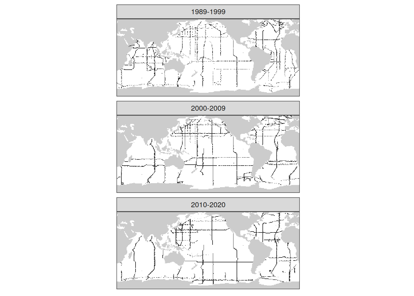
ggsave(plot = coverage_map,
       path = here::here("output/presentation"),
       filename = "Fig_observations_coverage_map.png",
       height = 6,
       width = 4)


GLODAP_all_coverage <- GLODAP_all %>%
  filter(between(depth, 250, 750)) %>%
  group_by(lat, lon, era) %>%
  summarise(tco2 = mean(tco2, na.rm = TRUE)) %>%
  ungroup()

map +
  geom_tile(data = GLODAP_all_coverage,
            aes(lon, lat, fill = tco2, col = tco2,
                height = 2, width = 2)) +
  facet_wrap( ~ era, ncol = 1) +
  scale_fill_viridis_c(name = expression(
    atop(DIC~at~"500m",(µmol~kg^{-1})))) +
  scale_color_viridis_c(guide = "none") +
  labs(title = "Observations",
       subtitle = "Decadal coverage") +
  theme(axis.text = element_blank(),
        axis.ticks = element_blank(),
        legend.position = "bottom")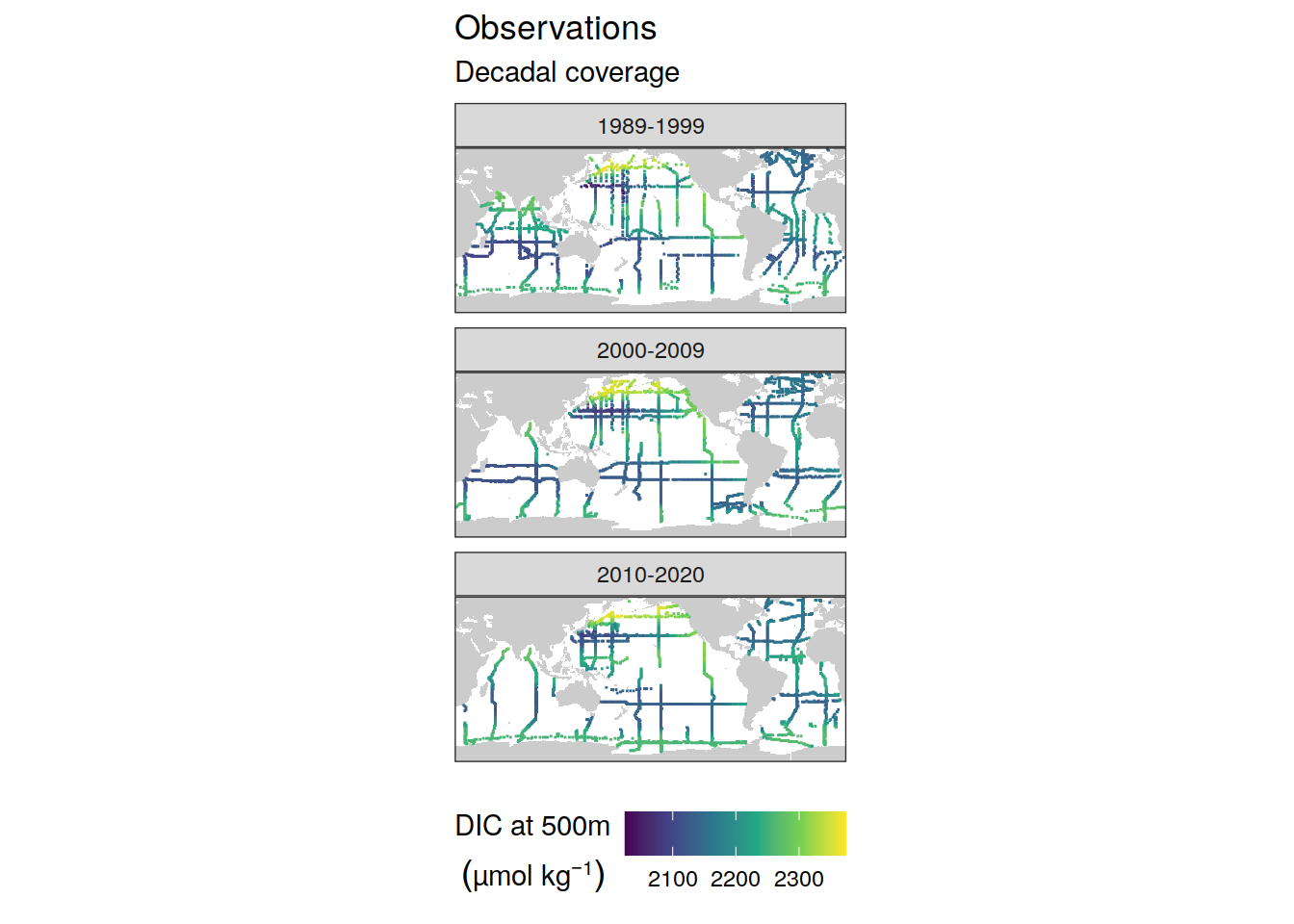
GLODAP_all_coverage_raster <- rast(GLODAP_all_coverage %>%
                                     relocate(lon, lat) %>%
                                     pivot_wider(names_from = era,
                                                 values_from = tco2),
                                   crs = "+proj=longlat")


GLODAP_all_coverage_raster <- project(GLODAP_all_coverage_raster, target_crs,
                                      method = "near")

GLODAP_all_coverage_tibble <- GLODAP_all_coverage_raster %>%
  as.data.frame(xy = TRUE, na.rm = FALSE) %>%
  as_tibble() %>%
  rename(lon = x, lat = y) %>%
  pivot_longer(cols = -c("lon", "lat"),
               names_to = "era",
               values_to = "tco2") %>%
  drop_na()

coverage_map <-
  ggplot() +
  geom_tile(data = GLODAP_all_coverage_tibble,
            aes(
              x = lon,
              y = lat,
              height = 3e5,
              width = 3e5,
              fill = tco2
            )) +
  geom_sf(data = worldmap_trans, fill = "grey90", col = "grey90") +
  geom_sf(data = coastline_trans, linewidth = 0.3) +
  geom_sf(data = bbox_graticules_trans, linewidth = 0.5) +
  coord_sf(
    crs = target_crs,
    ylim = lat_lim,
    xlim = lon_lim,
    expand = FALSE
  ) +
  scale_fill_viridis_c( expression(
    atop(DIC~at~"500m",(µmol~kg^{-1})))) +
  facet_wrap( ~ era, ncol = 1) +
  theme(
    axis.title = element_blank(),
    axis.text = element_blank(),
    axis.ticks = element_blank(),
    panel.border = element_rect(colour = "transparent"),
    strip.background = element_blank(),
    legend.position = "bottom"
  )


coverage_map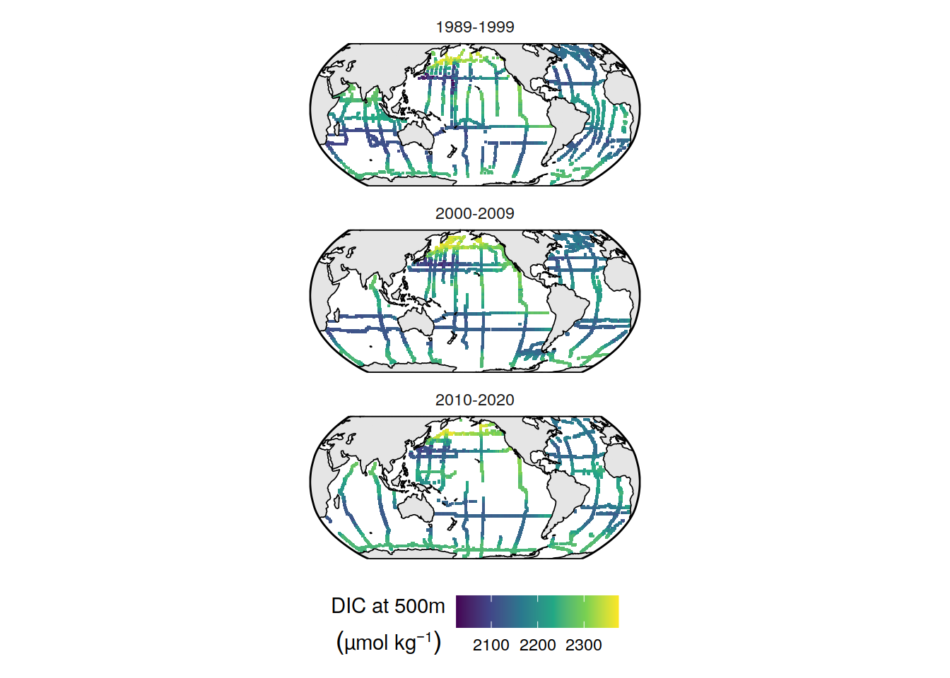
| Version | Author | Date |
|---|---|---|
| 2cca4eb | jens-daniel-mueller | 2023-01-10 |
ggsave(plot = coverage_map,
       path = here::here("output/presentation"),
       filename = "Fig_observations_coverage_map_dic.png",
       height = 6,
       width = 4,
       dpi = 600)

rm(coverage_map,
   GLODAP_all, GLODAP_all_coverage, GLODAP_expocodes,
   GLODAP_grid_era_all)

rm(cruises_phosphate_gap_fill,
   cruises_talk_gap_fill,
   cruises_talk_calc)
6 Atm CO2
co2_atm_roll <- co2_atm %>%
  mutate(pCO2_roll = zoo::rollmean(pCO2, 10, fill = NA))

p_pco2_atm <- co2_atm_roll %>%
  ggplot() +
  geom_point(aes(year, pCO2, col="annual")) +
  geom_path(aes(year, pCO2, col="annual")) +
  geom_point(aes(year, pCO2_roll, col="10yr roll")) +
  geom_path(aes(year, pCO2_roll, col="10yr roll"))

co2_atm_roll <- co2_atm_roll %>%
  mutate(delta_pCO2_roll = pCO2_roll - lag(pCO2_roll,10),
         delta_pCO2 = pCO2 - lag(pCO2,10))

p_delta_pCO2_atm <- co2_atm_roll %>%
  ggplot() +
  geom_point(aes(year, delta_pCO2, col="annual")) +
  geom_path(aes(year, delta_pCO2, col="annual")) +
  geom_point(aes(year, delta_pCO2_roll, col="10yr roll")) +
  geom_path(aes(year, delta_pCO2_roll, col="10yr roll"))

p_pco2_atm / p_delta_pCO2_atm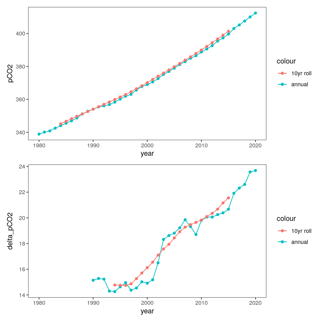
rm(p_pco2_atm, p_delta_pCO2_atm)

delta_pCO2_atm <-
  left_join(
    params_local_all %>%
      distinct(period, tref1, tref2),
    co2_atm_roll %>%
      select(
        tref1 = year,
        pCO2_1 = pCO2,
        pCO2_roll_1 = pCO2_roll
      )
  )

delta_pCO2_atm <-
  left_join(
    delta_pCO2_atm,
    co2_atm_roll %>%
      select(
        tref2 = year,
        pCO2_2 = pCO2,
        pCO2_roll_2 = pCO2_roll
      )
  )

delta_pCO2_atm <- delta_pCO2_atm %>%
  mutate(delta_pCO2 = pCO2_2 - pCO2_1,
         delta_pCO2_roll = pCO2_roll_2 - pCO2_roll_1) %>%
  select(period, delta_pCO2, delta_pCO2_roll)

delta_pCO2_atm <- delta_pCO2_atm %>%
  select(period, delta_pCO2)

delta_pCO2_atm <-
  bind_rows(
    delta_pCO2_atm,
    tibble(period = "1800 - 1994",
           delta_pCO2 = co2_atm %>% filter(year==1994) %>% pull(pCO2) - 280)
  )

rm(co2_atm_roll)
7 Globale scaling
- storage beneath 3000m: +2%
- unmapped regions south of 65N: +1.5%
- Nordic Seas: +1%
- Arctic Ocean: +2%
dcant_scaling <- 1.02*(1+0.02+0.015+0.01+0.003)
dcant_scaling_uncertainty <- 0.5
8 eMLR stats
8.1 Predictor selection
lm_best_predictor_counts_all %>%
  filter(period %in% two_decades,
         data_source == "obs") %>%
  pivot_longer(aou:temp,
               names_to = "predictor",
               values_to = "count") %>%
  # mutate(count = as.factor(count)) %>%
  group_by(predictor, count, period, Version_ID_group) %>%
  summarise(n = n()) %>%
  ungroup() %>%
  ggplot(aes(x = count, y = n)) +
  scale_color_manual(values = c("#EE7733", "#009988"), name = "Decade") +
  scale_fill_manual(values = c("#EE7733", "#009988"), name = "Decade") +
  geom_path(aes(col = period)) +
    geom_point(aes(fill = period), shape = 21) +
  coord_flip() +
  scale_x_continuous(breaks = seq(0,10,2),
                     limits = c(0,10),
                     name = "Presence among 10 best models") +
  labs(y = "Counts across density slabs, regional clusters and basins") +
  facet_wrap(~predictor)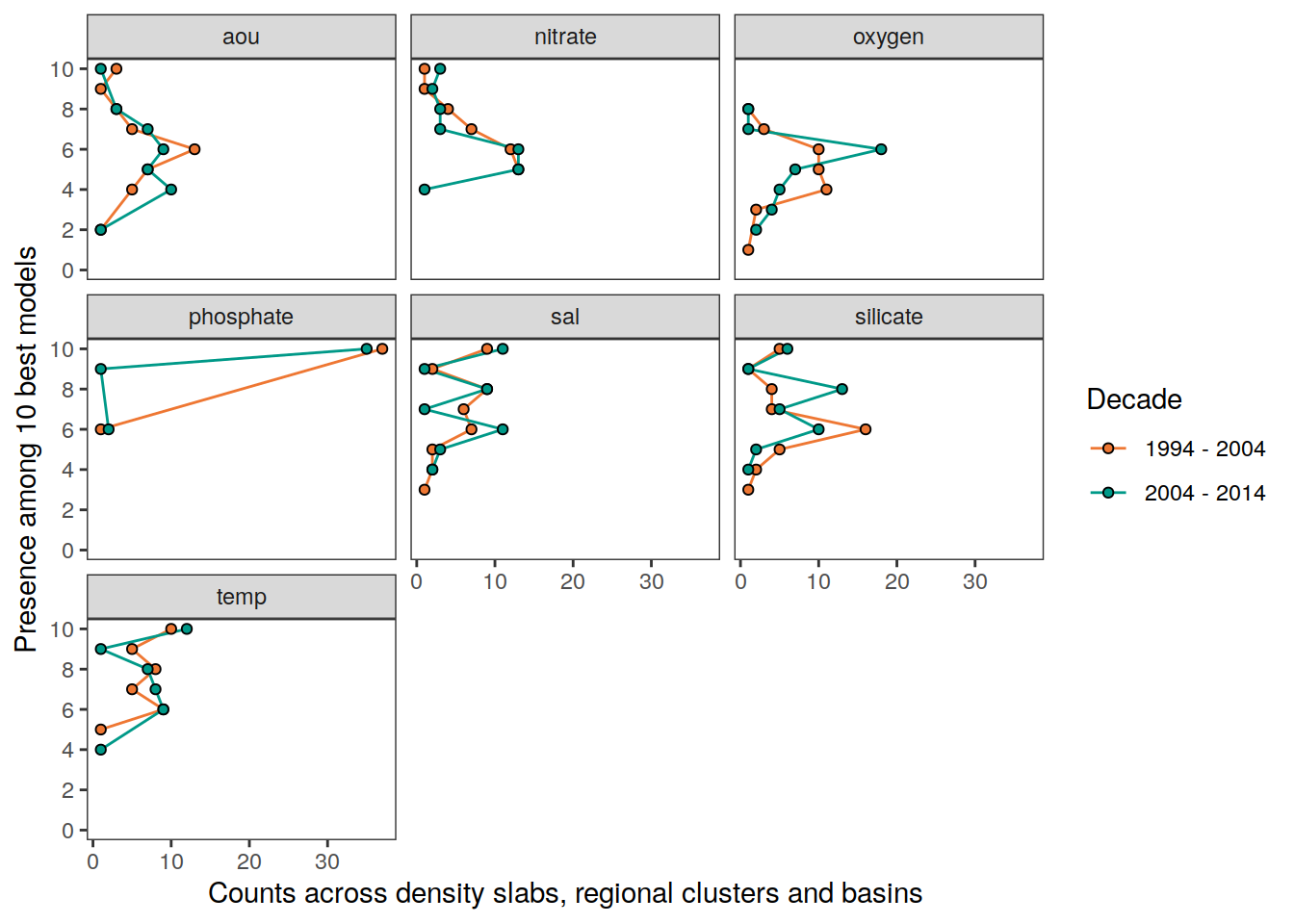
8.2 Residual distribution
spatial_residual_all %>%
  filter(gamma_slab %in% params_local$plot_slabs[2],
         data_source == "obs",
         period %in% two_decades) %>%
  p_map_dcant_slab(
    var = ".resid_mean",
    col = "divergent",
    title_text = "Residual distribution"
    ) +
  facet_grid(era ~ period) +
  theme_dark()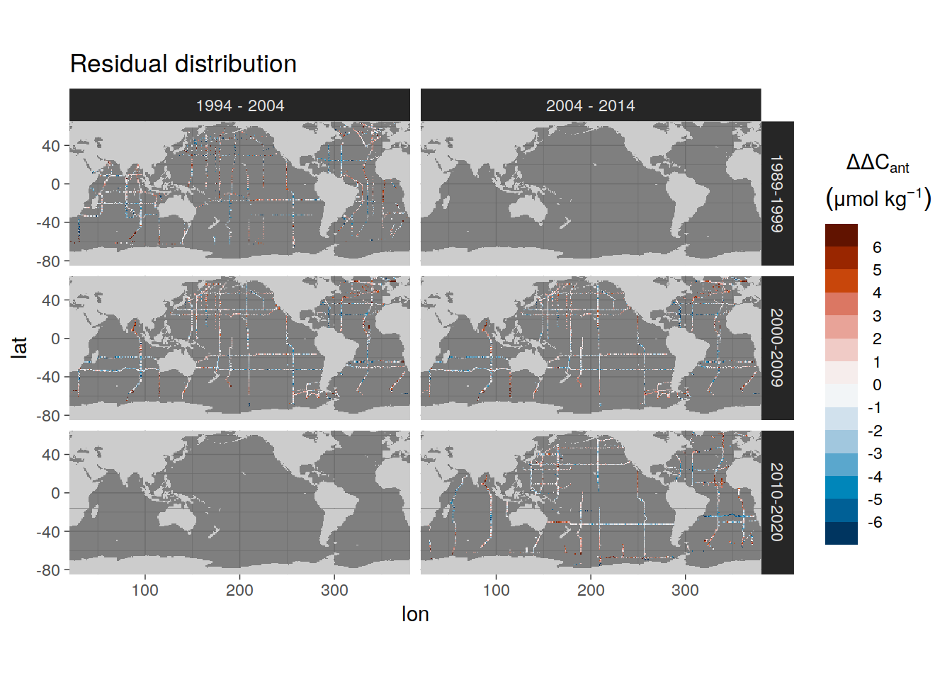
spatial_residual_offset_all %>%
  filter(
    gamma_slab %in% params_local$plot_slabs[1],
    data_source == "obs",
    period %in% two_decades
  ) %>%
  p_map_dcant_slab(var = ".resid_mean_offset",
                   col = "divergent",
                   title_text = "Residual offset distribution (era 2 - era 1)") +
  facet_grid(. ~ period) +
  theme_dark()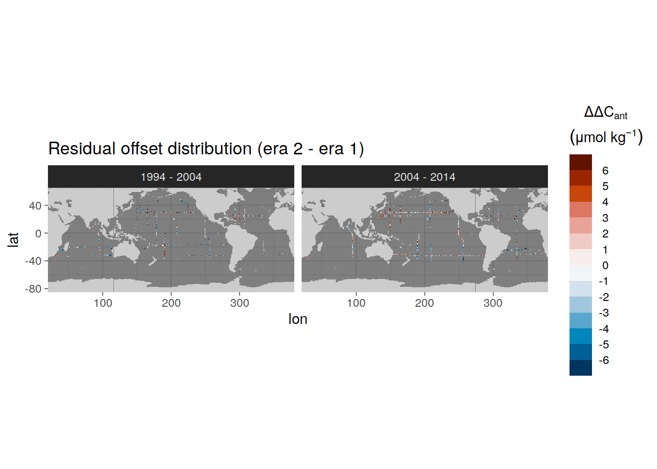
lat_residual_all %>%
  filter(data_source == "obs",
         period %in% two_decades) %>%
  ggplot(aes(
    .resid_mean,
    lat_grid,
    col = era,
    group = interaction(basin, era, gamma_slab, Version_ID)
  )) +
  geom_vline(xintercept = 0) +
  # geom_point() +
  geom_path(alpha = 0.5) +
  facet_grid(. ~ period)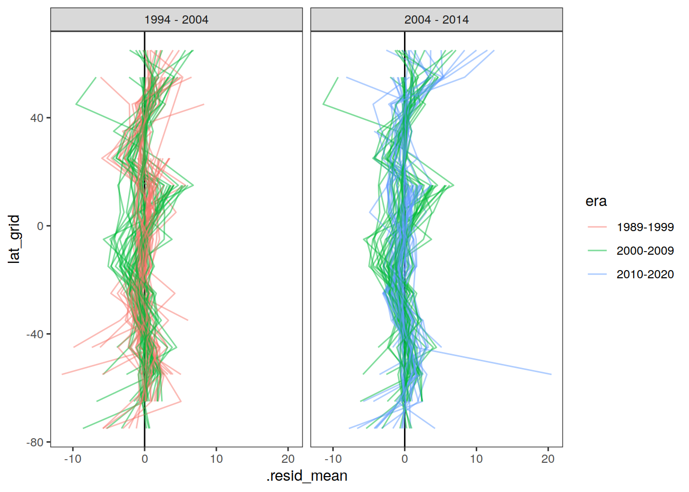
lat_residual_all %>%
filter(data_source == "obs",
period %in% two_decades) %>%
select(-c(Version_ID, tref1, tref2)) %>%
mutate(sampling_period = if_else(period == "2004 - 2014" &
era == "2000-2009",
"first",
"second"),
sampling_period = if_else(period == "1994 - 2004" &
era == "1989-1999",
"first",
sampling_period)) %>%
select(-era) %>%
pivot_wider(names_from = sampling_period,
values_from = .resid_mean) %>%
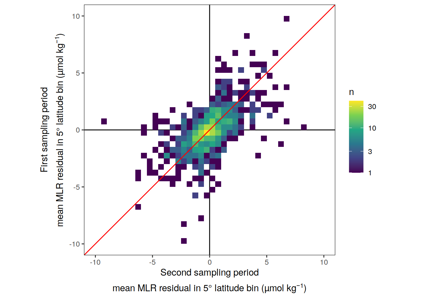
ggplot(aes(first, second)) +
geom_vline(xintercept = 0) +
geom_hline(yintercept = 0) +
geom_bin2d(binwidth = 0.5) +
geom_abline(slope = 1, col = "red") +
# geom_smooth(method = "lm") +
scale_fill_viridis_c(trans = "log10", name = "n") +
coord_fixed(ylim = c(-10, 10),
xlim = c(-10, 10)) +
labs(
y = expression(atop("First sampling period", "mean MLR residual in 5° latitude bin (µmol k"*g^{-1}*")")),
x = expression(atop("Second sampling period", "mean MLR residual in 5° latitude bin (µmol k"*g^{-1}*")"))
)
  # facet_wrap(~period)

ggsave(path = here::here("output/publication"),
       filename = "FigS_MLR_residual_correlation_latitude_bin.png",
       height = 5,
       width = 5,
       dpi = 600)


lat_residual_all %>%
  filter(data_source == "obs",
         period %in% two_decades) %>%
  select(-c(Version_ID, tref1, tref2)) %>%
  mutate(sampling_period = if_else(period == "2004 - 2014" &
                                     era == "2000-2009",
                                   "first",
                                   "second"),
         sampling_period = if_else(period == "1994 - 2004" &
                                     era == "1989-1999",
                                   "first",
                                   sampling_period)) %>%
  select(-era) %>%
  pivot_wider(names_from = sampling_period,
              values_from = .resid_mean) %>%
  nest_by(period) %>%
  mutate(mod = list(lm(second ~ first, data = data))) %>%
  summarize(broom::tidy(mod))
# A tibble: 4 × 6
# Groups: period [2]
period term estimate std.error statistic p.value
<chr> <chr> <dbl> <dbl> <dbl> <dbl>
1 1994 - 2004 (Intercept) -0.140 0.0842 -1.66 9.75e- 2
2 1994 - 2004 first 0.647 0.0465 13.9 2.23e-36
3 2004 - 2014 (Intercept) 0.142 0.0899 1.58 1.15e- 1
4 2004 - 2014 first 0.604 0.0415 14.6 3.76e-39lat_residual_all %>%
filter(data_source == "obs",
period %in% two_decades) %>%
select(-c(Version_ID, tref1, tref2)) %>%
mutate(sampling_period = if_else(period == "2004 - 2014" &
era == "2000-2009",
"first",
"second"),
sampling_period = if_else(period == "1994 - 2004" &
era == "1989-1999",
"first",
sampling_period)) %>%
select(-era) %>%
pivot_wider(names_from = sampling_period,
values_from = .resid_mean) %>%
drop_na() %>%
group_by(period) %>%
summarize(correlation = cor(first, second))# A tibble: 2 × 2
period correlation
<chr> <dbl>
1 1994 - 2004 0.566
2 2004 - 2014 0.580lat_residual_all_mean <- lat_residual_all %>%
filter(data_source == "obs",
period %in% two_decades) %>%
group_by(period, era, lat_grid) %>%
summarise(residual_mean = mean(abs(.resid_mean)),
residual_sd = sd(.resid_mean),
residual_iqr = IQR(.resid_mean)) %>%
ungroup()
lat_residual_offset_all_mean <- lat_residual_offset_all %>%
filter(data_source == "obs",
period %in% two_decades) %>%
group_by(period, lat_grid) %>%
summarise(residual_mean = mean(abs(.resid_mean_offset)),
residual_sd = sd(.resid_mean_offset),
residual_iqr = IQR(.resid_mean)) %>%
ungroup()
p_residual_lat <-
ggplot() +
geom_vline(xintercept = 0) +
geom_ribbon(
data = lat_residual_all_mean,
aes(
xmin = residual_mean - residual_iqr,
xmax = residual_mean + residual_iqr,
y = lat_grid,
fill = era
),
alpha = 0.3
) +
geom_path(data = lat_residual_all_mean,
aes(residual_mean,
lat_grid,
col = era)) +
scale_fill_highcontrast() +
scale_color_highcontrast() +
coord_cartesian(xlim = c(-3,7)) +
facet_grid(. ~ period)
p_residual_lat_offset <-
ggplot() +
geom_vline(xintercept = 0) +
geom_ribbon(
data = lat_residual_offset_all_mean,
aes(
xmin = residual_mean - residual_iqr,
xmax = residual_mean + residual_iqr,
y = lat_grid
),
alpha = 0.3
) +
geom_path(data = lat_residual_offset_all_mean,
aes(residual_mean,
lat_grid)) +
coord_cartesian(xlim = c(-3,7)) +
facet_grid(. ~ period)
p_residual_lat / p_residual_lat_offset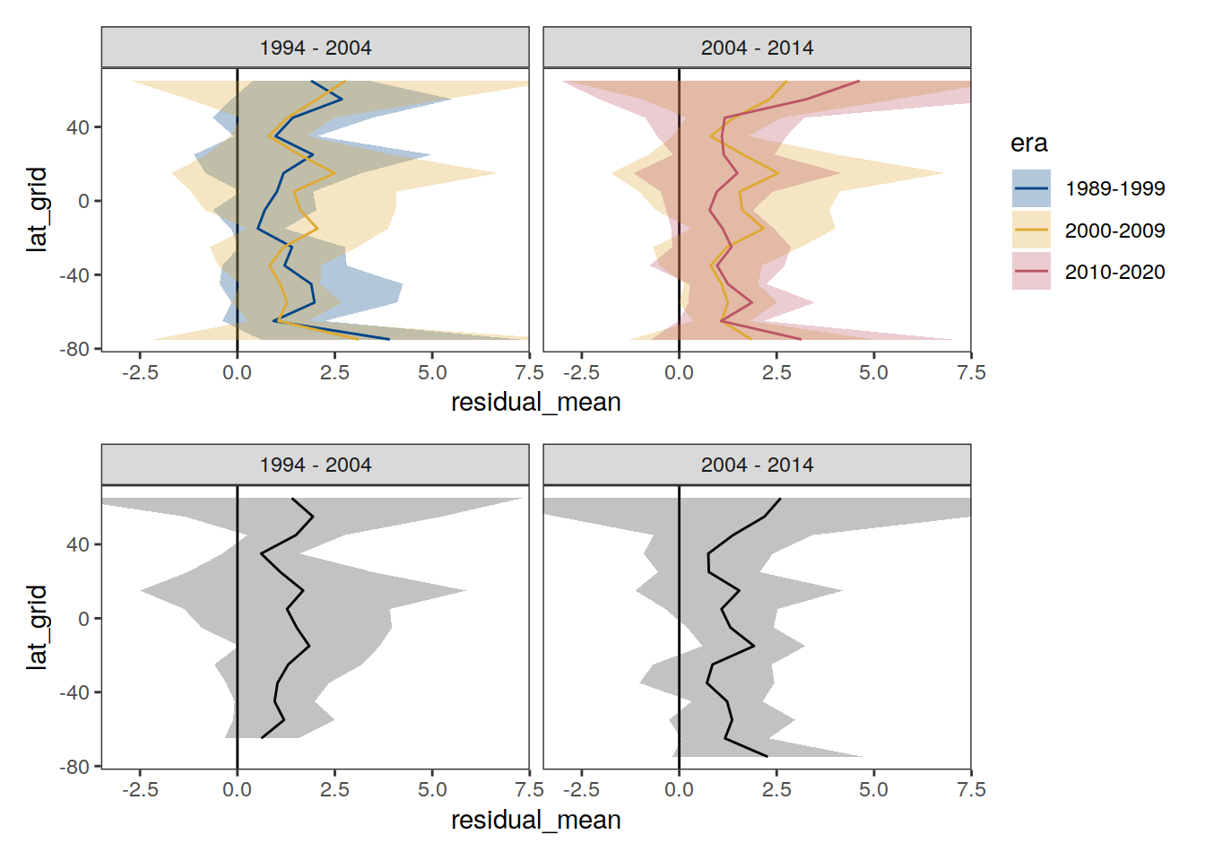
rm(p_residual_lat, p_residual_lat_offset)


p_residual_lat <-
ggplot() +
  geom_vline(xintercept = 0) +
  geom_path(data = lat_residual_all %>%
              filter(data_source == "obs",
                     period %in% two_decades,
                     gamma_slab %in% params_local$plot_slabs[2]),
            aes(.resid_mean,
                lat_grid,
                col = era)) +
  scale_fill_highcontrast() +
  scale_color_highcontrast() +
  coord_cartesian(xlim = c(-3,7)) +
  facet_grid(basin ~ period)

p_residual_lat_offset <-
ggplot() +
  geom_vline(xintercept = 0) +
  geom_path(data = lat_residual_offset_all %>%
              filter(data_source == "obs",
                     period %in% two_decades,
                     gamma_slab %in% params_local$plot_slabs[2]),
            aes(.resid_mean_offset,
                lat_grid)) +
  scale_fill_highcontrast() +
  scale_color_highcontrast() +
  coord_cartesian(xlim = c(-3,7)) +
  facet_grid(basin ~ period)


p_residual_lat / p_residual_lat_offset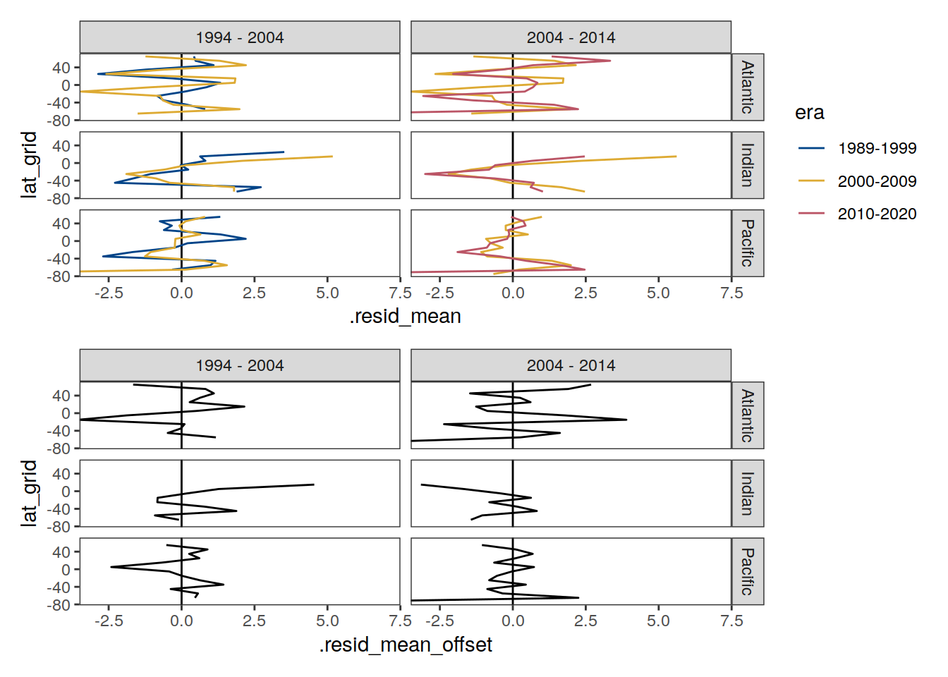
rm(p_residual_lat, p_residual_lat_offset)

lat_residual_offset_all %>%
  ggplot(aes(.resid_mean, .resid_mean_offset)) +
  geom_bin_2d() +
  scale_fill_viridis_c(trans = "log10")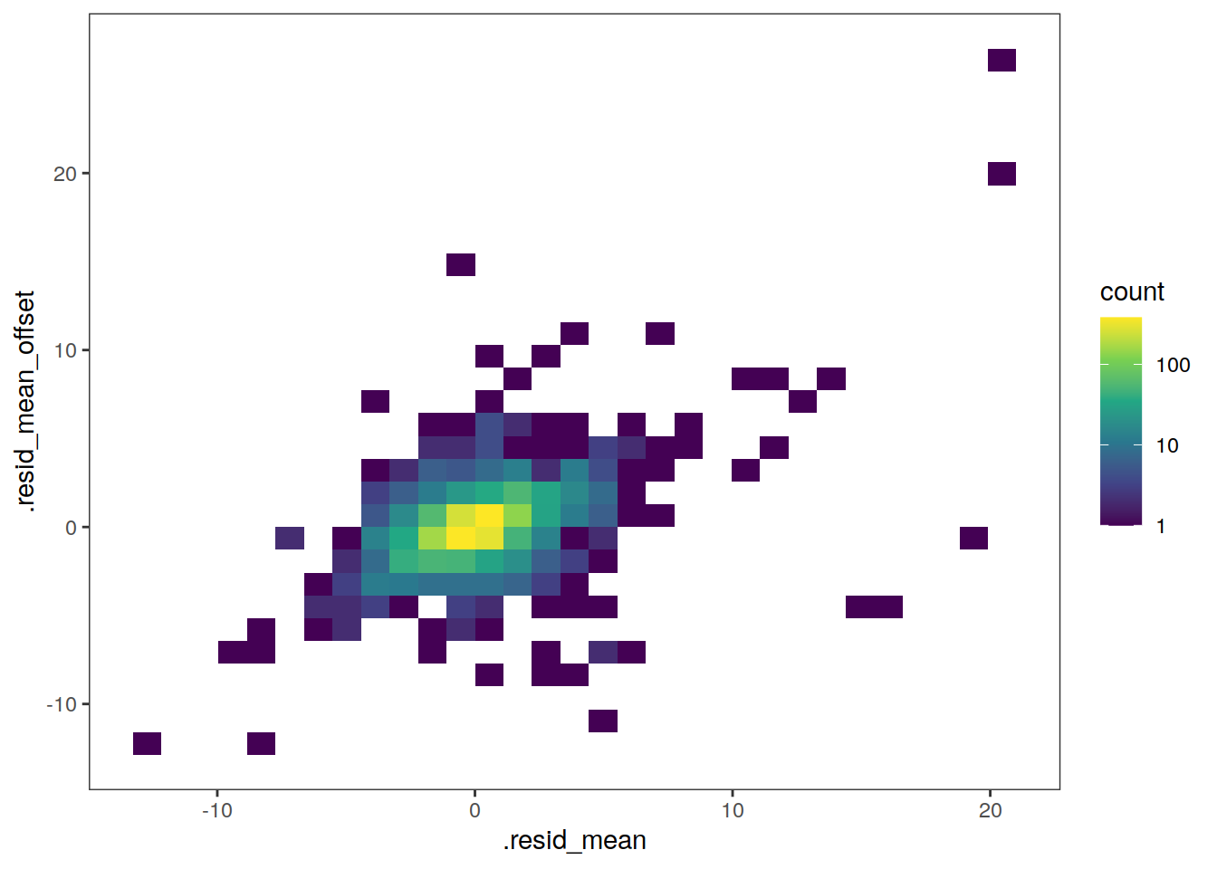
lat_residual_offset_all %>%
  pivot_longer(starts_with(".resid"),
               names_to = "type",
               values_to = "residual") %>%
  ggplot(aes(residual, fill = type, col = type)) +
  coord_cartesian(xlim = c(-5,5)) +
  geom_density(alpha = 0.5)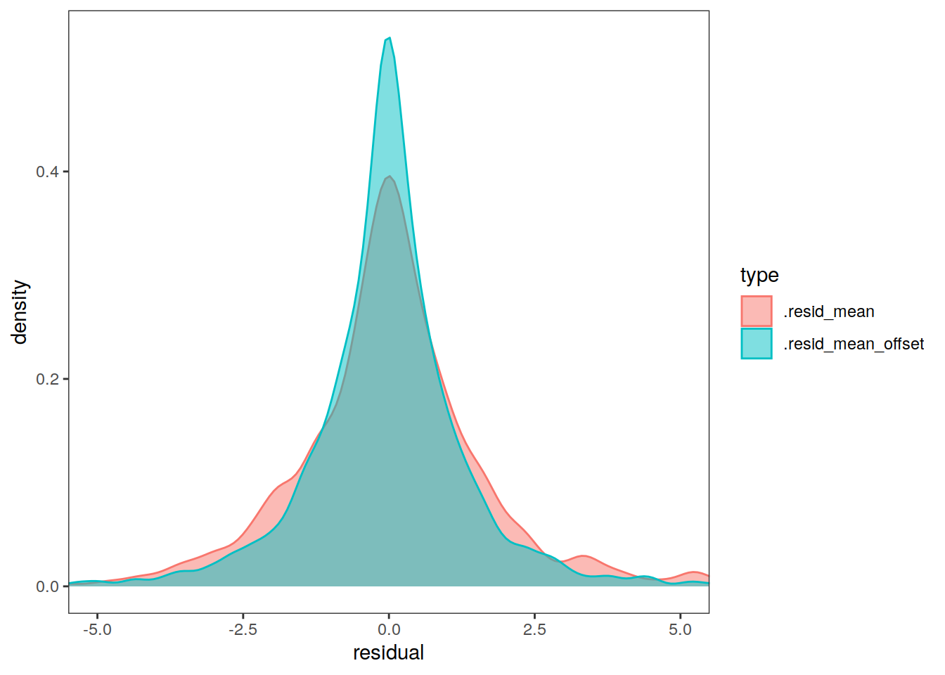
left_join(lm_best_target_all,
          GLODAP_glanced_all) %>%
  summarise(mean_rmse = mean(rmse, na.rm = TRUE),
            sd_rmse = sd(rmse, na.rm = TRUE))
# A tibble: 1 × 2
mean_rmse sd_rmse
<dbl> <dbl>
1 3.10 1.639 Column inventories
dcant_inv_all <- bind_rows(
  dcant_inv_all,
  tcant_inv %>% mutate(period = paste(tref1, tref2, sep = " - "),
                       data_source = "obs")
)


dcant_inv_all <- left_join(dcant_inv_all,
                           delta_pCO2_atm)


dcant_inv_all <- dcant_inv_all %>%
  mutate(beta = dcant / delta_pCO2,
         beta_pos = dcant_pos / delta_pCO2) %>%
  select(-starts_with("pCO2"))

dcant_inv_all_ensemble <- dcant_inv_all %>%
  filter(Version_ID %in% Version_IDs_ensemble_uncertainty)

dcant_inv_all_sensitivity <- dcant_inv_all %>%
  filter(Version_ID %in% Version_IDs_ensemble_sensitivity)

dcant_inv_all <- dcant_inv_all %>%
  filter(Version_ID %in% Version_IDs | is.na(Version_ID))
9.1 Sensitivity cases
dcant_inv_all_ensemble_sensitivity <-
  dcant_inv_all_sensitivity %>%
  filter(period %in% two_decades,
         data_source != "mod_truth") %>%
  select(lon, lat, period, data_source, MLR_basins, Version_ID_group, dcant)

dcant_inv_sensitivity <- additive_uncertainty(dcant_inv_all_ensemble_sensitivity)

delta_dcant_inv_sensitivity <- dcant_inv_sensitivity[[3]]
dcant_inv_sensitivity_contributions <- dcant_inv_sensitivity[[2]]
dcant_inv_sensitivity <- dcant_inv_sensitivity[[1]]


dcant_inv_sensitivity %>%
  mutate(
    data_source = case_when(
      data_source == "mod" ~ "Synthetic data",
      data_source == "obs" ~ "Observations"
    )
  ) %>%
  p_map_cant_inv(var = "sd",
                 breaks = c(seq(0, 16, 2), Inf),
                 title_text = NULL) +
  facet_grid(period ~ data_source) +
  theme(axis.text = element_blank(),
        axis.ticks = element_blank())
| Version | Author | Date |
|---|---|---|
| 3a7bab0 | jens-daniel-mueller | 2022-11-28 |
| 322b1c1 | jens-daniel-mueller | 2022-11-25 |
| 491f8b1 | jens-daniel-mueller | 2022-11-25 |
| 4da4d66 | jens-daniel-mueller | 2022-11-25 |
| e924c80 | jens-daniel-mueller | 2022-11-17 |
| 5520de8 | jens-daniel-mueller | 2022-11-15 |
| 375300e | jens-daniel-mueller | 2022-11-14 |
| cc337dd | jens-daniel-mueller | 2022-11-11 |
dcant_inv_sensitivity_contributions %>%
  filter(data_source == "obs",
         Version_ID_group != "Regional clustering") %>%
  rename(dcant_diff = sd) %>%
  p_map_cant_inv(var = "dcant_diff",
                 col = "bias",
                 breaks = c(-Inf, seq(-2,2,1), Inf),
                 title_text = NULL) +
  facet_grid(Version_ID_group ~ period) +
  theme(axis.text = element_blank(),
        axis.ticks = element_blank())
legend_title <- expression(atop(Delta * C["ant"] ~ offset,
                                (mol ~ m ^ {
                                  -2
                                } ~ dec ^ {
                                  -1
                                })))

p_map_mdim_robinson(
  df = dcant_inv_sensitivity_contributions %>%
    filter(data_source == "obs",
           Version_ID_group != "Regional clustering") %>%
    select(-data_source),
  dim_col = "period",
  dim_row = "Version_ID_group",
  var = "sd",
  breaks = c(-Inf, seq(-8, 8, 2), Inf),
  legend_title = legend_title,
  col = "divergent"
)
| Version | Author | Date |
|---|---|---|
| 8ded995 | jens-daniel-mueller | 2023-01-05 |
ggsave(path = here::here("output/publication"),
       filename = "FigS_dcant_column_inventory_uncertainty_sensitivity_cases.png",
       height = 8,
       width = 8,
       dpi = 600)
9.2 Uncertainty cases
dcant_inv_all_ensemble_uncertainty <-
  dcant_inv_all_ensemble %>%
  filter(period %in% two_decades,
         data_source != "mod_truth") %>%
  select(lon, lat, period, data_source, MLR_basins, Version_ID_group, dcant)

dcant_inv_uncertainty <- additive_uncertainty(dcant_inv_all_ensemble_uncertainty)

delta_dcant_inv_uncertainty <- dcant_inv_uncertainty[[3]]
dcant_inv_uncertainty_contributions <- dcant_inv_uncertainty[[2]]
dcant_inv_uncertainty <- dcant_inv_uncertainty[[1]]


dcant_inv_uncertainty %>%
  filter(data_source == "obs") %>%
  mutate(
    data_source = case_when(
      data_source == "mod" ~ "Synthetic data",
      data_source == "obs" ~ "Observations"
    )
  ) %>%
  p_map_cant_inv(var = "sd",
                 breaks = c(seq(0, 8, 1), Inf),
                 title_text = NULL) +
  facet_grid(. ~ period) +
  theme(axis.text = element_blank(),
        axis.ticks = element_blank())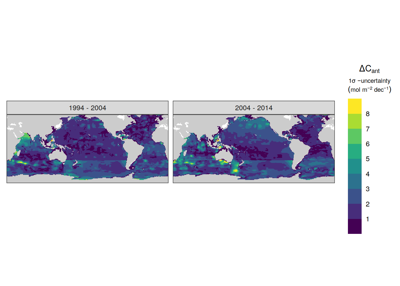
| Version | Author | Date |
|---|---|---|
| 0f2c9d5 | jens-daniel-mueller | 2022-12-08 |
| 3a7bab0 | jens-daniel-mueller | 2022-11-28 |
| 322b1c1 | jens-daniel-mueller | 2022-11-25 |
| 491f8b1 | jens-daniel-mueller | 2022-11-25 |
| 4da4d66 | jens-daniel-mueller | 2022-11-25 |
| 534ee74 | jens-daniel-mueller | 2022-11-25 |
| 57d1a9b | jens-daniel-mueller | 2022-11-17 |
| e924c80 | jens-daniel-mueller | 2022-11-17 |
| 5520de8 | jens-daniel-mueller | 2022-11-15 |
| 1dad51a | jens-daniel-mueller | 2022-11-15 |
| cc337dd | jens-daniel-mueller | 2022-11-11 |
legend_title <- expression(atop(Delta * C["ant"],
                                atop("1" * sigma ~ -uncertainty,
                                     (mol ~ m ^ {
                                       -2
                                     } ~ dec ^ {
                                       -1
                                     }))))

p_map_mdim_robinson(
  df = dcant_inv_uncertainty %>%
    filter(data_source == "obs") %>%
    select(lon, lat, period, sd),
  dim_col = "period",
  var = "sd",
  breaks = c(seq(0, 8, 1), Inf),
  legend_title = legend_title
)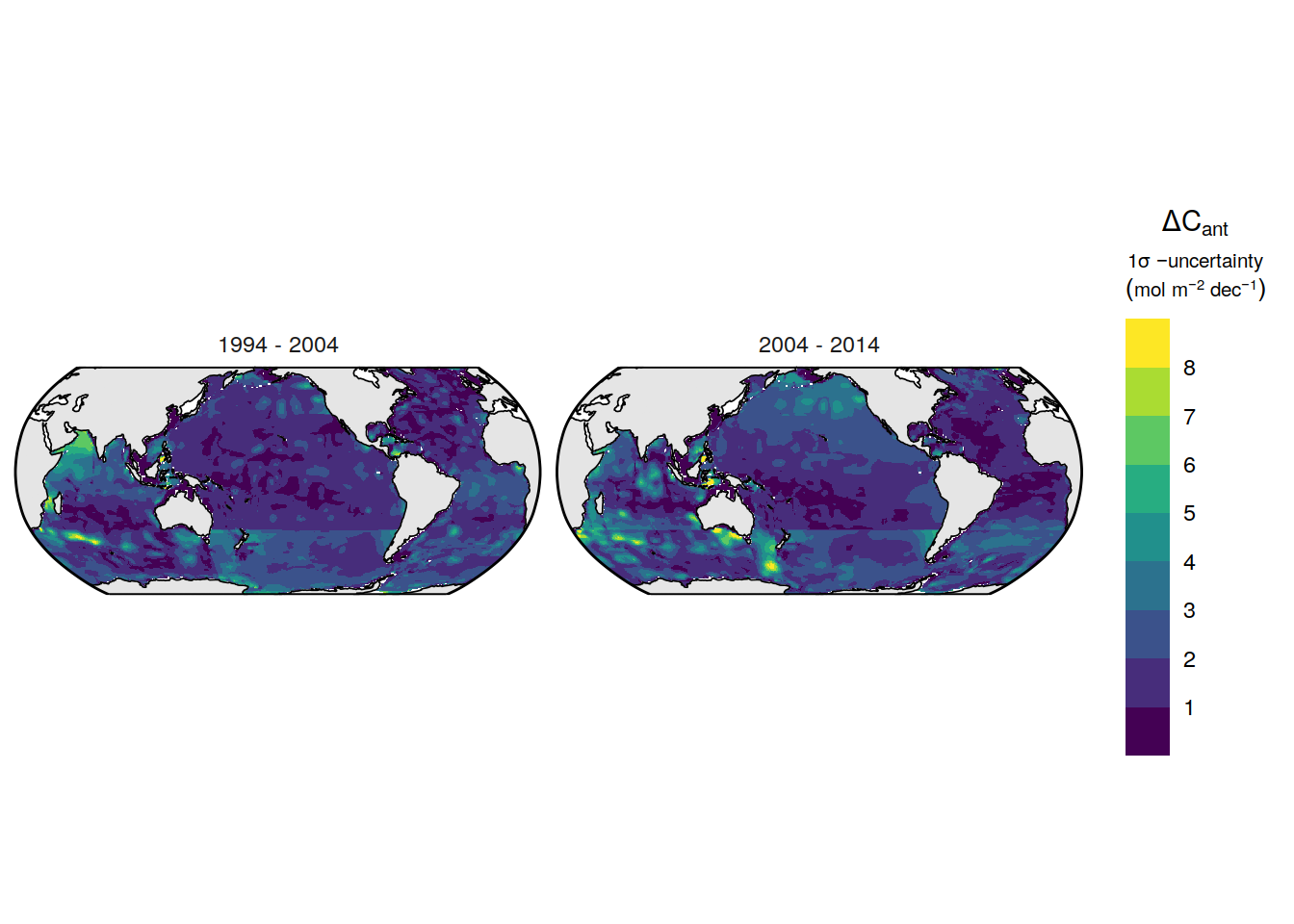
| Version | Author | Date |
|---|---|---|
| 8ded995 | jens-daniel-mueller | 2023-01-05 |
| 0f2c9d5 | jens-daniel-mueller | 2022-12-08 |
| 3a7bab0 | jens-daniel-mueller | 2022-11-28 |
| 534ee74 | jens-daniel-mueller | 2022-11-25 |
| e924c80 | jens-daniel-mueller | 2022-11-17 |
| 5520de8 | jens-daniel-mueller | 2022-11-15 |
| 1dad51a | jens-daniel-mueller | 2022-11-15 |
| cc337dd | jens-daniel-mueller | 2022-11-11 |
ggsave(path = here::here("output/publication"),
       filename = "FigS_dcant_column_inventory_uncertainty.png",
       height = 3.5,
       width = 8,
       dpi = 600)

dcant_inv_uncertainty_contributions %>%
  filter(data_source == "obs") %>%
  mutate(
    data_source = case_when(
      data_source == "mod" ~ "Synthetic data",
      data_source == "obs" ~ "Observations"
    )
  ) %>%
  rename(dcant_diff_uncertainty = sd) %>%
  p_map_cant_inv(var = "dcant_diff_uncertainty",
                 col = "bias",
                 breaks = c(-Inf, seq(-2,2,1), Inf),
                 title_text = NULL) +
  facet_grid(Version_ID_group ~ period) +
  theme(axis.text = element_blank(),
        axis.ticks = element_blank())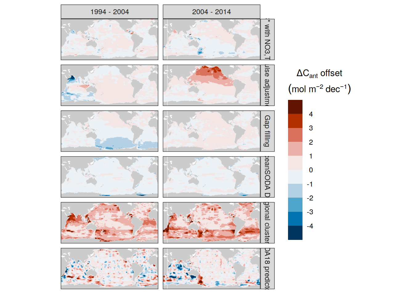
| Version | Author | Date |
|---|---|---|
| 8ded995 | jens-daniel-mueller | 2023-01-05 |
legend_title <- expression(atop(Delta * C["ant"] ~ offset,
                                (mol ~ m ^ {
                                  -2
                                } ~ dec ^ {
                                  -1
                                })))

p_map_mdim_robinson(
  df = dcant_inv_uncertainty_contributions %>%
    filter(data_source == "obs") %>%
    select(-data_source),
  dim_col = "period",
  dim_row = "Version_ID_group",
  var = "sd",
  breaks = c(-Inf, seq(-4, 4, 1), Inf),
  legend_title = legend_title,
  col = "divergent"
)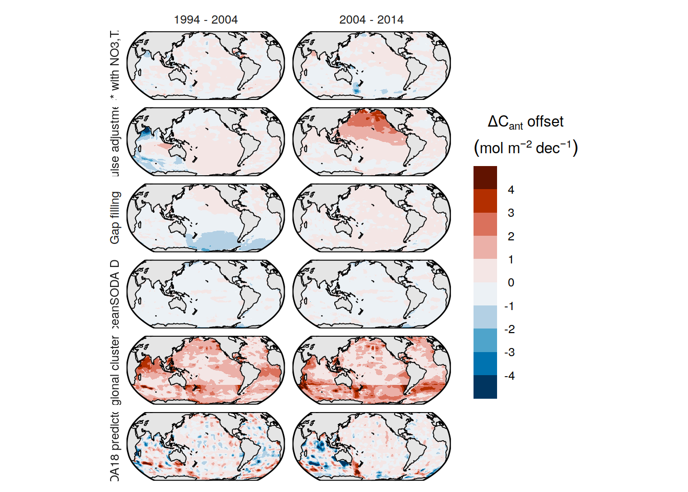
| Version | Author | Date |
|---|---|---|
| 8ded995 | jens-daniel-mueller | 2023-01-05 |
ggsave(path = here::here("output/publication"),
       filename = "FigS_dcant_column_inventory_uncertainty_contributions.png",
       height = 9,
       width = 8,
       dpi = 600)
dcant_inv_all_ensemble_uncertainty <-
dcant_inv_all_ensemble %>%
filter(period %in% two_decades,
data_source != "mod_truth") %>%
select(lon, lat, period, data_source, MLR_basins, Version_ID_group, dcant)
dcant_inv_all_ensemble_uncertainty <-
m_grid_horizontal_coarse(dcant_inv_all_ensemble_uncertainty)
dcant_inv_all_ensemble_uncertainty <-
dcant_inv_all_ensemble_uncertainty %>%
group_by(lat_grid, lon_grid, data_source, period, MLR_basins, Version_ID_group) %>%
summarise(dcant = mean(dcant),
n = n()) %>%
ungroup() %>%
filter(n == 25) %>%
rename(lon = lon_grid,
lat = lat_grid)
dcant_inv_uncertainty <- additive_uncertainty(dcant_inv_all_ensemble_uncertainty)
delta_dcant_inv_uncertainty <- dcant_inv_uncertainty[[3]]
dcant_inv_uncertainty_contributions <- dcant_inv_uncertainty[[2]]
dcant_inv_uncertainty <- dcant_inv_uncertainty[[1]]
dcant_inv_uncertainty %>%
mutate(
data_source = case_when(
data_source == "mod" ~ "Synthetic data",
data_source == "obs" ~ "Observations"
)
) %>%
p_map_cant_inv(var = "sd",
breaks = c(seq(0, 8, 1), Inf),
title_text = NULL) +
facet_grid(period ~ data_source) +
theme(axis.text = element_blank(),
axis.ticks = element_blank())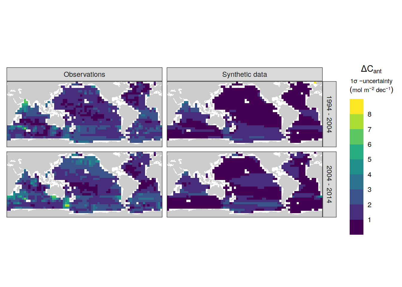
| Version | Author | Date |
|---|---|---|
| 3a7bab0 | jens-daniel-mueller | 2022-11-28 |
| 322b1c1 | jens-daniel-mueller | 2022-11-25 |
| 491f8b1 | jens-daniel-mueller | 2022-11-25 |
| 4da4d66 | jens-daniel-mueller | 2022-11-25 |
| 534ee74 | jens-daniel-mueller | 2022-11-25 |
| e924c80 | jens-daniel-mueller | 2022-11-17 |
| 5520de8 | jens-daniel-mueller | 2022-11-15 |
| 1dad51a | jens-daniel-mueller | 2022-11-15 |
| cc337dd | jens-daniel-mueller | 2022-11-11 |
delta_dcant_inv_uncertainty %>%
  p_map_cant_inv(var = "delta_dcant",
                 col = "bias",
                 title_text = NULL) +
  facet_grid(data_source ~ .) +
  theme(axis.text = element_blank(),
        axis.ticks = element_blank())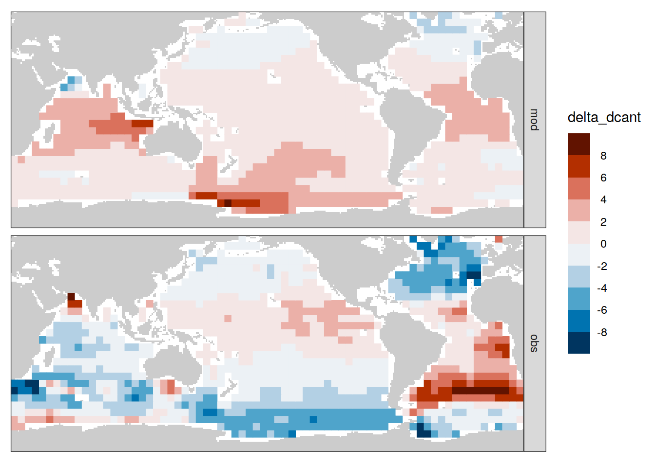
delta_dcant_inv_uncertainty %>%
  p_map_cant_inv(var = "RSS",
                 breaks = c(seq(0, 8, 1), Inf),
                 title_text = NULL) +
  facet_grid(data_source ~ .) +
  theme(axis.text = element_blank(),
        axis.ticks = element_blank())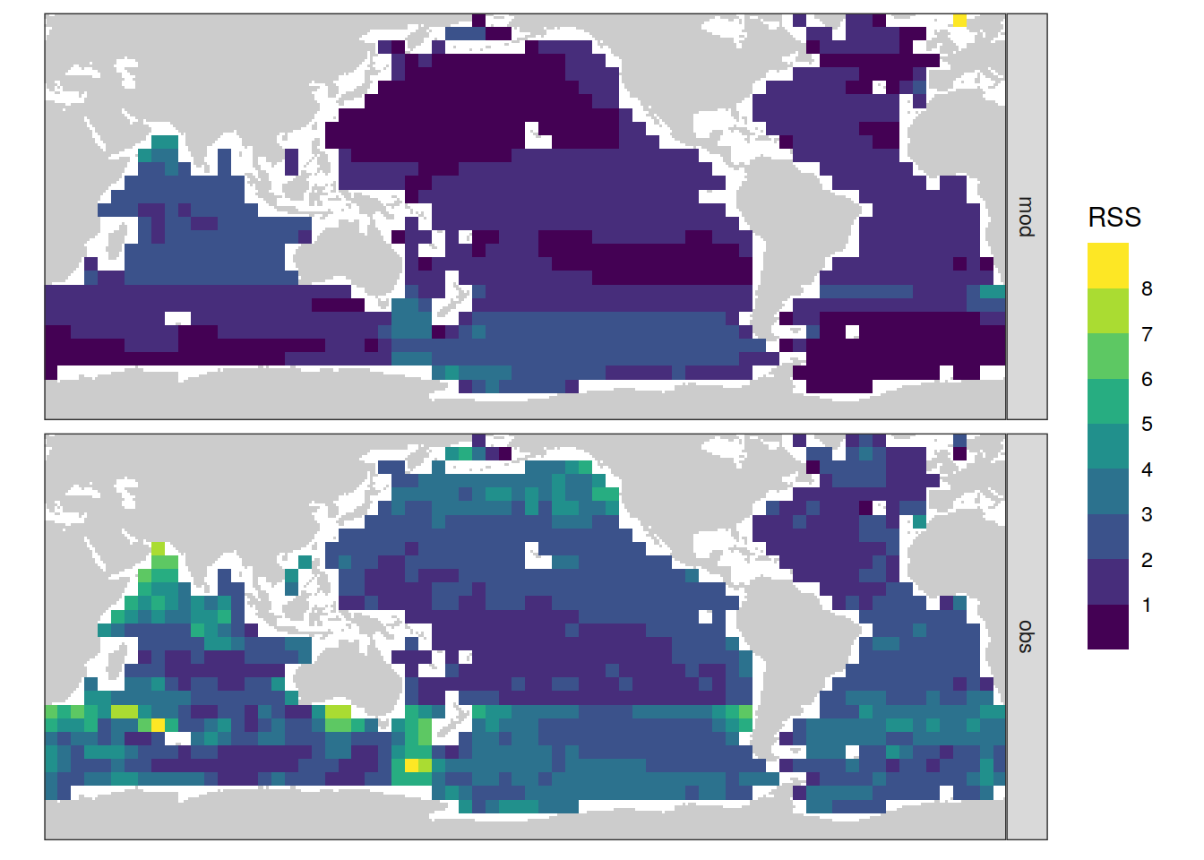
delta_dcant_inv_uncertainty %>%
  filter(signif_single == 1) %>%
  p_map_cant_inv(var = "delta_dcant",
                 col = "bias",
                 title_text = NULL) +
  facet_grid(data_source ~ .) +
  theme(axis.text = element_blank(),
        axis.ticks = element_blank())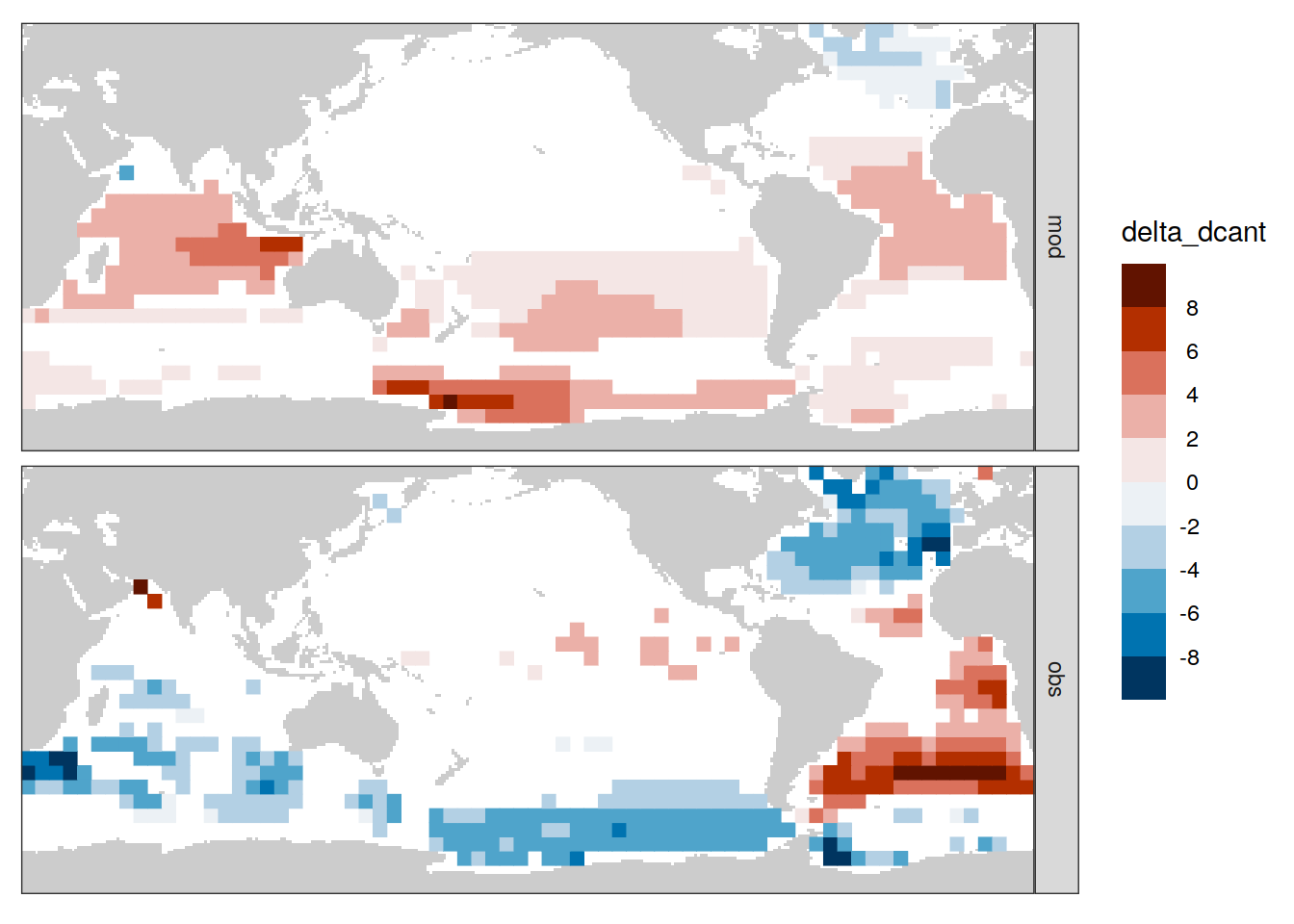
| Version | Author | Date |
|---|---|---|
| 8ded995 | jens-daniel-mueller | 2023-01-05 |
| 3a7bab0 | jens-daniel-mueller | 2022-11-28 |
| 322b1c1 | jens-daniel-mueller | 2022-11-25 |
| 491f8b1 | jens-daniel-mueller | 2022-11-25 |
| 4da4d66 | jens-daniel-mueller | 2022-11-25 |
| 534ee74 | jens-daniel-mueller | 2022-11-25 |
| 1dad51a | jens-daniel-mueller | 2022-11-15 |
| cc337dd | jens-daniel-mueller | 2022-11-11 |
delta_dcant_inv_uncertainty %>%
  filter(signif_double == 1) %>%
  p_map_cant_inv(var = "delta_dcant",
                 col = "bias",
                 title_text = NULL) +
  facet_grid(data_source ~ .) +
  theme(axis.text = element_blank(),
        axis.ticks = element_blank())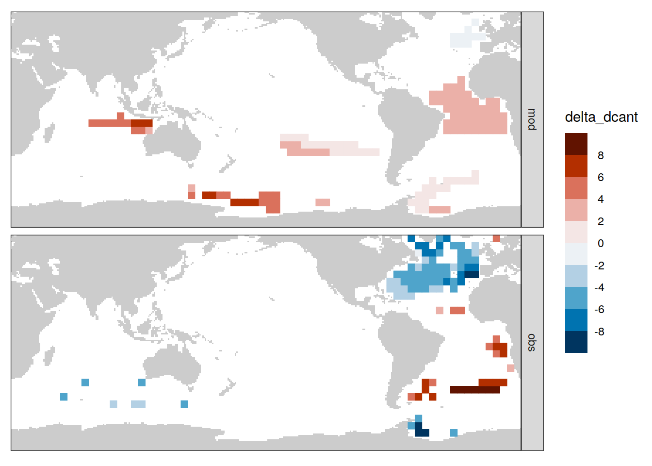
9.3 dCant - absolute
p_CI_absolute <- dcant_inv_all %>%
  filter(period %in% two_decades,
         data_source %in% c("obs")) %>%
  p_map_cant_inv(var = "dcant",
                 title_text = NULL) +
  facet_wrap(~ period, ncol = 1) +
  theme(axis.text.x = element_blank()) +
  geom_point(
    data = dcant_inv_uncertainty %>%
      filter(signif_double == 0,
             data_source == "obs"),
    aes(lon, lat),
    shape = 20,
    size = 0.1,
    col = "grey"
  ) +
    geom_point(
    data = dcant_inv_uncertainty %>%
      filter(signif_single == 0,
             data_source == "obs"),
    aes(lon, lat),
    shape = 20,
    size = 1,
    col = "grey"
  )

p_CI_absolute +
  theme(axis.text = element_blank(),
        axis.ticks = element_blank())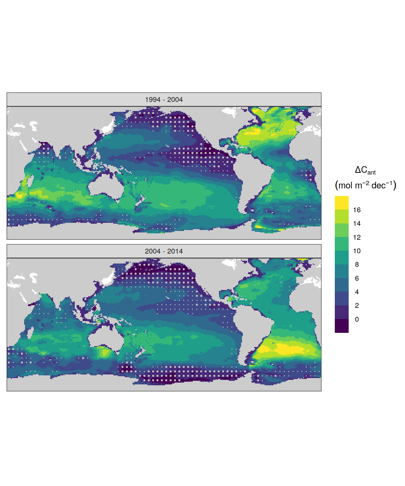
| Version | Author | Date |
|---|---|---|
| 3a7bab0 | jens-daniel-mueller | 2022-11-28 |
| 322b1c1 | jens-daniel-mueller | 2022-11-25 |
| 491f8b1 | jens-daniel-mueller | 2022-11-25 |
| 4da4d66 | jens-daniel-mueller | 2022-11-25 |
| 534ee74 | jens-daniel-mueller | 2022-11-25 |
| 5520de8 | jens-daniel-mueller | 2022-11-15 |
| 1dad51a | jens-daniel-mueller | 2022-11-15 |
| 6edad9b | jens-daniel-mueller | 2022-11-11 |
| 16beb51 | jens-daniel-mueller | 2022-11-08 |
| b92657d | jens-daniel-mueller | 2022-11-08 |
| 7275091 | jens-daniel-mueller | 2022-11-05 |
dcant_inv_uncertainty %>%
  select(data_source, lon, lat, period, starts_with("signif")) %>%
  mutate(area = earth_surf(lat,lon)) %>%
  group_by(data_source, period, signif_single) %>%
  summarize(area_signif = sum(area)) %>%
  ungroup() %>%
  group_by(data_source, period) %>%
  mutate(area_total = sum(area_signif)) %>%
  ungroup() %>%
  mutate(area_fraction = 100 * area_signif / area_total)
# A tibble: 12 × 6
data_source period signif_single area_signif area_total area_fraction
<chr> <chr> <dbl> <dbl> <dbl> <dbl>
1 mod 1994 - 2004 0 2.67e11 1.11e13 2.40
2 mod 1994 - 2004 1 1.09e13 1.11e13 97.5
3 mod 1994 - 2004 NA 1.65e10 1.11e13 0.148
4 mod 2004 - 2014 0 3.57e10 1.11e13 0.320
5 mod 2004 - 2014 1 1.11e13 1.11e13 99.5
6 mod 2004 - 2014 NA 1.65e10 1.11e13 0.148
7 obs 1994 - 2004 0 8.74e11 1.13e13 7.76
8 obs 1994 - 2004 1 1.04e13 1.13e13 92.2
9 obs 1994 - 2004 NA 9.81e 9 1.13e13 0.0872
10 obs 2004 - 2014 0 1.07e12 1.13e13 9.48
11 obs 2004 - 2014 1 1.02e13 1.13e13 90.4
12 obs 2004 - 2014 NA 9.81e 9 1.13e13 0.08729.4 Inventory stats
9.4.1 Basin
dcant_inv_stat_mean <-
  full_join(basinmask,
            dcant_inv_all) %>%
  mutate(surf_area = earth_surf(lat, lon)) %>%
  group_by(basin, period, data_source) %>%
  summarise(dcant = weighted.mean(dcant, surf_area)) %>%
  ungroup() %>%
  filter(!is.na(dcant))

dcant_inv_stat_ensemble <-
  full_join(basinmask,
            dcant_inv_all_ensemble) %>%
  mutate(surf_area = earth_surf(lat, lon)) %>%
  group_by(basin, data_source, period, MLR_basins, Version_ID_group) %>%
  summarise(dcant = weighted.mean(dcant, surf_area)) %>%
  ungroup() %>%
  filter(!is.na(dcant)) %>%
  group_by(basin, data_source, period) %>%
  summarise(dcant_sd = sd(dcant) * 2) %>%
  ungroup()

dcant_inv_stat <-
  full_join(dcant_inv_stat_mean,
            dcant_inv_stat_ensemble)

rm(dcant_inv_stat_mean,
   dcant_inv_stat_ensemble)

dcant_inv_stat %>%
  filter(period %in% two_decades) %>%
  group_by(data_source, basin) %>%
  mutate(delta_dcant = dcant - lag(dcant),
         RSS = sqrt(dcant_sd ^ 2 + lag(dcant_sd ^ 2))) %>%
  ungroup() %>%
  kable() %>%
  kable_styling() %>%
scroll_box(height = "300px")| basin | period | data_source | dcant | dcant_sd | delta_dcant | RSS |
|---|---|---|---|---|---|---|
| N. Pacific | 1994 - 2004 | mod | 3.363703 | 0.3712442 | NA | NA |
| N. Pacific | 1994 - 2004 | mod_truth | 2.915800 | 0.0000000 | NA | NA |
| N. Pacific | 1994 - 2004 | obs | 3.076873 | 1.8983189 | NA | NA |
| N. Pacific | 2004 - 2014 | mod | 3.614817 | 0.4403483 | 0.2511143 | 0.5759591 |
| N. Pacific | 2004 - 2014 | mod_truth | 3.352012 | 0.0000000 | 0.4362120 | 0.0000000 |
| N. Pacific | 2004 - 2014 | obs | 3.415398 | 1.5195985 | 0.3385254 | 2.4316238 |
| S. Pacific | 1994 - 2004 | mod | 4.826130 | 1.2656840 | NA | NA |
| S. Pacific | 1994 - 2004 | mod_truth | 4.931744 | 0.0000000 | NA | NA |
| S. Pacific | 1994 - 2004 | obs | 7.482479 | 1.3015988 | NA | NA |
| S. Pacific | 2004 - 2014 | mod | 6.476528 | 0.8515919 | 1.6503976 | 1.5255048 |
| S. Pacific | 2004 - 2014 | mod_truth | 6.060215 | 0.0000000 | 1.1284704 | 0.0000000 |
| S. Pacific | 2004 - 2014 | obs | 6.402648 | 1.5413944 | -1.0798310 | 2.0174380 |
| N. Atlantic | 1994 - 2004 | mod | 4.616514 | 0.9132060 | NA | NA |
| N. Atlantic | 1994 - 2004 | mod_truth | 4.057536 | 0.0000000 | NA | NA |
| N. Atlantic | 1994 - 2004 | obs | 9.867769 | 0.6490727 | NA | NA |
| N. Atlantic | 2004 - 2014 | mod | 5.075378 | 0.6845292 | 0.4588643 | 1.1412823 |
| N. Atlantic | 2004 - 2014 | mod_truth | 4.878549 | 0.0000000 | 0.8210126 | 0.0000000 |
| N. Atlantic | 2004 - 2014 | obs | 8.025765 | 1.5821054 | -1.8420048 | 1.7100740 |
| S. Atlantic | 1994 - 2004 | mod | 5.064488 | 0.9895347 | NA | NA |
| S. Atlantic | 1994 - 2004 | mod_truth | 4.706655 | 0.0000000 | NA | NA |
| S. Atlantic | 1994 - 2004 | obs | 7.252470 | 1.6530468 | NA | NA |
| S. Atlantic | 2004 - 2014 | mod | 6.393315 | 0.7347411 | 1.3288264 | 1.2324867 |
| S. Atlantic | 2004 - 2014 | mod_truth | 5.251166 | 0.0000000 | 0.5445113 | 0.0000000 |
| S. Atlantic | 2004 - 2014 | obs | 9.960798 | 2.0284147 | 2.7083280 | 2.6166830 |
| Indian | 1994 - 2004 | mod | 5.899824 | 2.1898564 | NA | NA |
| Indian | 1994 - 2004 | mod_truth | 5.570926 | 0.0000000 | NA | NA |
| Indian | 1994 - 2004 | obs | 8.154922 | 1.5925219 | NA | NA |
| Indian | 2004 - 2014 | mod | 7.583920 | 1.2120903 | 1.6840960 | 2.5029251 |
| Indian | 2004 - 2014 | mod_truth | 6.501337 | 0.0000000 | 0.9304108 | 0.0000000 |
| Indian | 2004 - 2014 | obs | 6.519972 | 0.7627870 | -1.6349503 | 1.7657775 |
9.4.2 Gyres
dcant_inv_stat_ensemble <-
  full_join(basinmask,
            dcant_inv_all_ensemble) %>%
  mutate(surf_area = earth_surf(lat, lon),
         lat_grid = cut(lat, c(-50, -20, 20, 50))) %>%
  group_by(basin,
           data_source,
           period,
           MLR_basins,
           Version_ID_group,
           lat_grid) %>%
  summarise(dcant = weighted.mean(dcant, surf_area)) %>%
  ungroup() %>%
  filter(!is.na(dcant),
         !is.na(lat_grid),
         lat_grid != "(-20,20]")

dcant_inv_stat_uncertainty <- additive_uncertainty(dcant_inv_stat_ensemble %>%
                                                     filter(period %in% two_decades))

delta_dcant_inv_stat_uncertainty <- dcant_inv_stat_uncertainty[[3]]
dcant_inv_stat_uncertainty <- dcant_inv_stat_uncertainty[[1]]


dcant_inv_stat_uncertainty %>%
  filter(data_source == "obs") %>%
  kable() %>%
  kable_styling() %>%
scroll_box(height = "300px")| basin | data_source | period | lat_grid | sd | std_case | signif_single | signif_double |
|---|---|---|---|---|---|---|---|
| N. Pacific | obs | 1994 - 2004 | (20,50] | 0.9900593 | 3.9829040 | 1 | 1 |
| N. Pacific | obs | 2004 - 2014 | (20,50] | 2.3041469 | 3.3833004 | 1 | 0 |
| S. Pacific | obs | 1994 - 2004 | (-50,-20] | 1.4359046 | 9.8048932 | 1 | 1 |
| S. Pacific | obs | 2004 - 2014 | (-50,-20] | 1.1921319 | 8.5667582 | 1 | 1 |
| N. Atlantic | obs | 1994 - 2004 | (20,50] | 0.5388493 | 12.1361324 | 1 | 1 |
| N. Atlantic | obs | 2004 - 2014 | (20,50] | 0.6289353 | 8.4461849 | 1 | 1 |
| S. Atlantic | obs | 1994 - 2004 | (-50,-20] | 0.9183569 | 8.4912458 | 1 | 1 |
| S. Atlantic | obs | 2004 - 2014 | (-50,-20] | 1.9497286 | 13.1557314 | 1 | 1 |
| Indian | obs | 1994 - 2004 | (-50,-20] | 0.7599534 | 10.7970711 | 1 | 1 |
| Indian | obs | 1994 - 2004 | (20,50] | 4.2501720 | -0.3174586 | 0 | 0 |
| Indian | obs | 2004 - 2014 | (-50,-20] | 1.0554965 | 8.2468486 | 1 | 1 |
| Indian | obs | 2004 - 2014 | (20,50] | 2.1877358 | 7.0876343 | 1 | 1 |
delta_dcant_inv_stat_uncertainty %>%
  filter(data_source == "obs") %>%
  kable() %>%
  kable_styling() %>%
scroll_box(height = "300px")| basin | data_source | period | lat_grid | sd | std_case | delta_dcant | RSS | signif_single | signif_double |
|---|---|---|---|---|---|---|---|---|---|
| N. Pacific | obs | 2004 - 2014 | (20,50] | 2.3041469 | 3.383300 | -0.5996036 | 2.5078498 | 0 | 0 |
| S. Pacific | obs | 2004 - 2014 | (-50,-20] | 1.1921319 | 8.566758 | -1.2381350 | 1.8662799 | 0 | 0 |
| N. Atlantic | obs | 2004 - 2014 | (20,50] | 0.6289353 | 8.446185 | -3.6899474 | 0.8282018 | 1 | 1 |
| S. Atlantic | obs | 2004 - 2014 | (-50,-20] | 1.9497286 | 13.155731 | 4.6644856 | 2.1551847 | 1 | 1 |
| Indian | obs | 2004 - 2014 | (-50,-20] | 1.0554965 | 8.246849 | -2.5502226 | 1.3006160 | 1 | 0 |
| Indian | obs | 2004 - 2014 | (20,50] | 2.1877358 | 7.087634 | 7.4050929 | 4.7801830 | 1 | 0 |
rm(dcant_inv_stat_ensemble,
   dcant_inv_stat_uncertainty,
   delta_dcant_inv_stat_uncertainty)
dcant_inv_all %>%
filter(period %in% two_decades,
data_source != "obs") %>%
mutate(
data_source = case_when(
data_source == "mod" ~ "Reconstruction",
data_source == "mod_truth" ~ "Model truth"
)
) %>%
p_map_cant_inv(var = "dcant",
title_text = NULL) +
facet_grid(period ~ data_source) +
theme(axis.text.x = element_blank())
| Version | Author | Date |
|---|---|---|
| 8ded995 | jens-daniel-mueller | 2023-01-05 |
| 0f2c9d5 | jens-daniel-mueller | 2022-12-08 |
| 3a7bab0 | jens-daniel-mueller | 2022-11-28 |
| 322b1c1 | jens-daniel-mueller | 2022-11-25 |
| 491f8b1 | jens-daniel-mueller | 2022-11-25 |
| 4da4d66 | jens-daniel-mueller | 2022-11-25 |
| 534ee74 | jens-daniel-mueller | 2022-11-25 |
| 5520de8 | jens-daniel-mueller | 2022-11-15 |
| 1dad51a | jens-daniel-mueller | 2022-11-15 |
| 6edad9b | jens-daniel-mueller | 2022-11-11 |
| 16beb51 | jens-daniel-mueller | 2022-11-08 |
| b92657d | jens-daniel-mueller | 2022-11-08 |
| 7275091 | jens-daniel-mueller | 2022-11-05 |
legend_title <- expression(atop(Delta * C["ant"],
                                (mol ~ m ^ {
                                  -2
                                } ~ dec ^ {
                                  -1
                                })))

p_CI_absolute_mod_delta <- p_map_mdim_robinson(
  df = dcant_inv_all %>%
    filter(period %in% two_decades,
           data_source != "obs") %>%
    mutate(
      data_source = case_when(
        data_source == "mod" ~ "Reconstruction",
        data_source == "mod_truth" ~ "Model truth"
      )
    ) %>%
    select(lon, lat, period, data_source, dcant),
  dim_row = "period",
  dim_col = "data_source",
  var = "dcant",
  legend_title = legend_title
)

dcant_inv_all %>%
  filter(period %in% two_decades,
         data_source != "obs") %>%
  select(data_source, lon, lat, basin_AIP, period, dcant) %>%
  pivot_wider(names_from = period,
              values_from = dcant) %>%
  mutate(dcant_offset = `2004 - 2014` - `1994 - 2004`,
         period = "Decadal offset") %>%
  mutate(
    data_source = case_when(
      data_source == "mod" ~ "Reconstruction",
      data_source == "mod_truth" ~ "Model truth"
    )
  ) %>%
  p_map_cant_inv(
    var = "dcant_offset",
    title_text = NULL,
    subtitle_text = NULL,
    col = "bias"
  ) +
  facet_grid(. ~ data_source)
        legend_title <- expression(atop(Delta * Delta * C["ant"],
                                        (mol ~ m ^ {-2}~dec^{-1})))

p_CI_bias_delta <- p_map_mdim_robinson(
  df = dcant_inv_all %>%
    filter(period %in% two_decades,
           data_source != "obs") %>%
    select(data_source, lon, lat, basin_AIP, period, dcant) %>%
    pivot_wider(names_from = period,
                values_from = dcant) %>%
    mutate(dcant_offset = `2004 - 2014` - `1994 - 2004`,
           period = "Decadal offset") %>%
    mutate(
      data_source = case_when(
        data_source == "mod" ~ "Reconstruction",
        data_source == "mod_truth" ~ "Model truth"
      )
    ) %>%
    select(lon, lat, data_source, dcant_offset),
  dim_col = "data_source",
  var = "dcant_offset",
  breaks = c(-Inf, seq(-8, 8, 2), Inf),
  legend_title = legend_title,
  col = "divergent"
)

p_CI_absolute_mod_delta / p_CI_bias_delta +
  plot_annotation(tag_levels = 'A')
| Version | Author | Date |
|---|---|---|
| 8ded995 | jens-daniel-mueller | 2023-01-05 |
ggsave(path = here::here("output/publication"),
       filename = "FigS_delta_dcant_column_inventory_synthetic_data.png",
       height = 7,
       width = 8,
       dpi = 600)

rm(p_CI_absolute_mod_delta, p_CI_bias_delta)
9.5 dCant - delta
delta_dcant_inv_all <-
  dcant_inv_all %>%
  filter(data_source %in% c("obs", "mod"),
         period %in% two_decades) %>%
  select(data_source, lon, lat, basin_AIP, period, dcant) %>%
  pivot_wider(names_from = period,
              values_from = dcant) %>%
  mutate(dcant_offset = `2004 - 2014` - `1994 - 2004`,
         period = "(2004 - 2014) - (1994 - 2004)")

p_CI_delta <-
  delta_dcant_inv_all %>%
  filter(data_source == "obs") %>%
  p_map_cant_inv(
    var = "dcant_offset",
    title_text = NULL,
    subtitle_text = NULL,
    col = "bias"
  ) +
  geom_point(
    data = delta_dcant_inv_uncertainty %>%
      filter(signif_single == 0,
             data_source == "obs") %>%
      mutate(period = "(2004 - 2014) - (1994 - 2004)"),
    aes(lon, lat),
    shape = 20,
    size = 1,
    col = "black"
  ) +
  geom_point(
    data = delta_dcant_inv_uncertainty %>%
      filter(signif_double == 0,
             data_source == "obs") %>%
      mutate(period = "(2004 - 2014) - (1994 - 2004)"),
    aes(lon, lat),
    shape = 20,
    size = 0.1,
    col = "black"
  ) +
  facet_wrap(~ period)

p_CI_absolute / p_CI_delta +
  plot_annotation(tag_levels = 'A')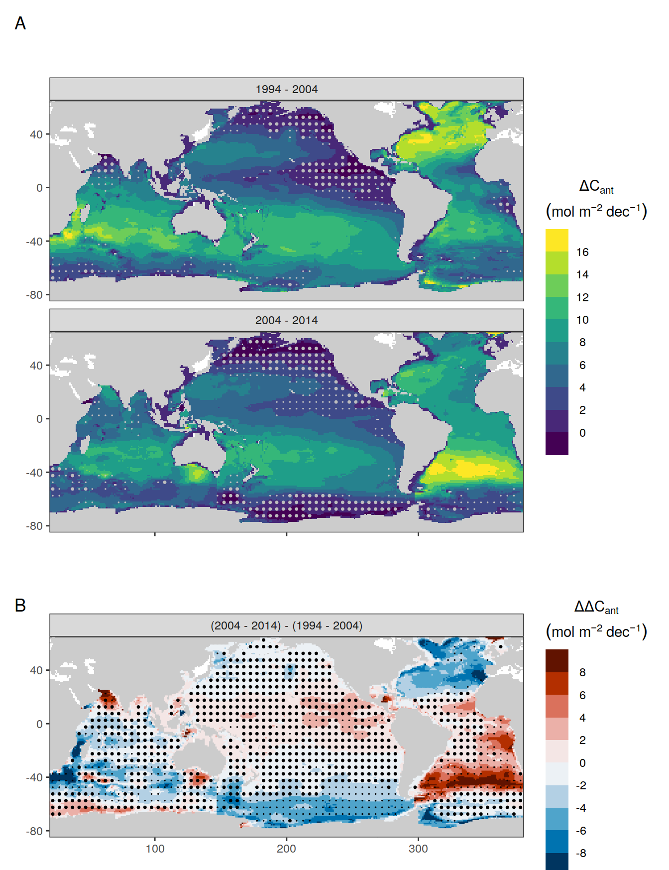
| Version | Author | Date |
|---|---|---|
| 8ded995 | jens-daniel-mueller | 2023-01-05 |
| 3a7bab0 | jens-daniel-mueller | 2022-11-28 |
| 322b1c1 | jens-daniel-mueller | 2022-11-25 |
| 491f8b1 | jens-daniel-mueller | 2022-11-25 |
| 4da4d66 | jens-daniel-mueller | 2022-11-25 |
| 534ee74 | jens-daniel-mueller | 2022-11-25 |
| 5520de8 | jens-daniel-mueller | 2022-11-15 |
| 1dad51a | jens-daniel-mueller | 2022-11-15 |
| 6edad9b | jens-daniel-mueller | 2022-11-11 |
| 16beb51 | jens-daniel-mueller | 2022-11-08 |
| b92657d | jens-daniel-mueller | 2022-11-08 |
| 7275091 | jens-daniel-mueller | 2022-11-05 |
| 2345935 | jens-daniel-mueller | 2022-10-29 |
| 051b911 | jens-daniel-mueller | 2022-09-07 |
| 75bd58c | jens-daniel-mueller | 2022-09-07 |
| 1c6de0d | jens-daniel-mueller | 2022-09-07 |
| 78dbb27 | jens-daniel-mueller | 2022-08-11 |
| 302d289 | jens-daniel-mueller | 2022-08-11 |
| e2adac6 | jens-daniel-mueller | 2022-07-22 |
| fea41c1 | jens-daniel-mueller | 2022-07-20 |
| d2ae54c | jens-daniel-mueller | 2022-07-18 |
| ea46812 | jens-daniel-mueller | 2022-07-13 |
| f09080e | jens-daniel-mueller | 2022-06-28 |
| 16dc3af | jens-daniel-mueller | 2022-06-27 |
| 87e9eb8 | jens-daniel-mueller | 2022-06-27 |
| b52b159 | jens-daniel-mueller | 2022-06-27 |
| 1d73ec9 | jens-daniel-mueller | 2022-05-16 |
| 2ca0109 | jens-daniel-mueller | 2022-05-02 |
| b018a9a | jens-daniel-mueller | 2022-04-29 |
| e09320d | jens-daniel-mueller | 2022-04-12 |
| acad2e2 | jens-daniel-mueller | 2022-04-09 |
| 3d81135 | jens-daniel-mueller | 2022-04-07 |
| a74e341 | jens-daniel-mueller | 2022-04-04 |
| bd9e11d | jens-daniel-mueller | 2022-03-22 |
| 2501978 | jens-daniel-mueller | 2022-03-21 |
| 094bfa0 | jens-daniel-mueller | 2022-02-18 |
| d2191ad | jens-daniel-mueller | 2022-02-04 |
| 5f2aed0 | jens-daniel-mueller | 2022-01-27 |
| 9753eb8 | jens-daniel-mueller | 2022-01-26 |
| b1d7720 | jens-daniel-mueller | 2022-01-21 |
| d6b399a | jens-daniel-mueller | 2022-01-21 |
p_CI_delta +
  theme(axis.text = element_blank(),
        axis.ticks = element_blank())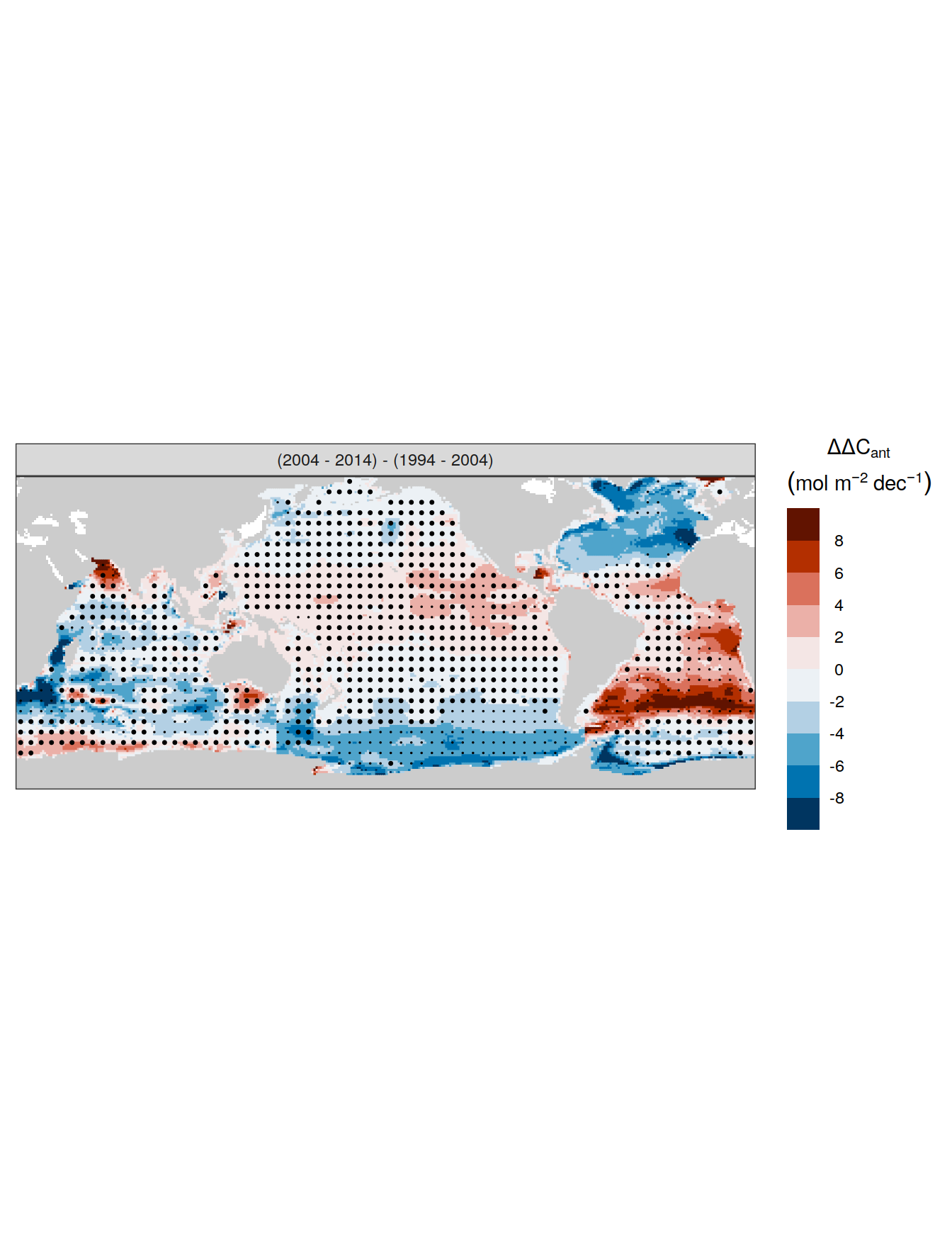
| Version | Author | Date |
|---|---|---|
| 8ded995 | jens-daniel-mueller | 2023-01-05 |
| 3a7bab0 | jens-daniel-mueller | 2022-11-28 |
| 322b1c1 | jens-daniel-mueller | 2022-11-25 |
| 491f8b1 | jens-daniel-mueller | 2022-11-25 |
| 4da4d66 | jens-daniel-mueller | 2022-11-25 |
| 534ee74 | jens-daniel-mueller | 2022-11-25 |
| 5520de8 | jens-daniel-mueller | 2022-11-15 |
| 1dad51a | jens-daniel-mueller | 2022-11-15 |
| 6edad9b | jens-daniel-mueller | 2022-11-11 |
| 16beb51 | jens-daniel-mueller | 2022-11-08 |
| b92657d | jens-daniel-mueller | 2022-11-08 |
| 7275091 | jens-daniel-mueller | 2022-11-05 |
| 2345935 | jens-daniel-mueller | 2022-10-29 |
| 051b911 | jens-daniel-mueller | 2022-09-07 |
| 75bd58c | jens-daniel-mueller | 2022-09-07 |
| 1c6de0d | jens-daniel-mueller | 2022-09-07 |
| 78dbb27 | jens-daniel-mueller | 2022-08-11 |
| 302d289 | jens-daniel-mueller | 2022-08-11 |
| e2adac6 | jens-daniel-mueller | 2022-07-22 |
| fea41c1 | jens-daniel-mueller | 2022-07-20 |
| d2ae54c | jens-daniel-mueller | 2022-07-18 |
| ea46812 | jens-daniel-mueller | 2022-07-13 |
| f09080e | jens-daniel-mueller | 2022-06-28 |
| 16dc3af | jens-daniel-mueller | 2022-06-27 |
| 87e9eb8 | jens-daniel-mueller | 2022-06-27 |
| b52b159 | jens-daniel-mueller | 2022-06-27 |
| 1d73ec9 | jens-daniel-mueller | 2022-05-16 |
| 2ca0109 | jens-daniel-mueller | 2022-05-02 |
| b018a9a | jens-daniel-mueller | 2022-04-29 |
| e09320d | jens-daniel-mueller | 2022-04-12 |
| acad2e2 | jens-daniel-mueller | 2022-04-09 |
| 3d81135 | jens-daniel-mueller | 2022-04-07 |
| a74e341 | jens-daniel-mueller | 2022-04-04 |
| bd9e11d | jens-daniel-mueller | 2022-03-22 |
| 2501978 | jens-daniel-mueller | 2022-03-21 |
| 094bfa0 | jens-daniel-mueller | 2022-02-18 |
| d2191ad | jens-daniel-mueller | 2022-02-04 |
| 5f2aed0 | jens-daniel-mueller | 2022-01-27 |
| 9753eb8 | jens-daniel-mueller | 2022-01-26 |
| b1d7720 | jens-daniel-mueller | 2022-01-21 |
| d6b399a | jens-daniel-mueller | 2022-01-21 |
ggsave(path = here::here("output/presentation"),
       filename = "Fig_dcant_column_inventory_delta.png",
       height = 3.2,
       width = 6)

rm(p_CI_absolute, p_CI_delta)
dcant_inv_dec1 <- dcant_inv_all %>%
filter(data_source == "obs",
period == "1994 - 2004") %>%
select(lon, lat, dcant)
dcant_inv_dec2 <- dcant_inv_all %>%
filter(data_source == "obs",
period == "2004 - 2014") %>%
select(lon, lat, dcant)
delta_dcant_inv <- delta_dcant_inv_all %>%
filter(data_source == "obs") %>%
select(lon, lat, dcant_offset)
dcant_inv_uncert_dec1 <- dcant_inv_uncertainty %>%
filter(data_source == "obs",
period == "1994 - 2004") %>%
select(lon, lat, signif_single, signif_double) %>%
st_as_sf(coords = c("lon", "lat"), crs = "+proj=longlat")
dcant_inv_uncert_dec2 <- dcant_inv_uncertainty %>%
filter(data_source == "obs",
period == "2004 - 2014") %>%
select(lon, lat, signif_single, signif_double) %>%
st_as_sf(coords = c("lon", "lat"), crs = "+proj=longlat")
dcant_inv_uncert_delta <- delta_dcant_inv_uncertainty %>%
filter(data_source == "obs") %>%
select(lon, lat, signif_single, signif_double) %>%
st_as_sf(coords = c("lon", "lat"), crs = "+proj=longlat")
legend_title <- expression(atop(Delta * C["ant"],
(mol ~ m ^ {
-2
} ~ dec ^ {
-1
})))
p_dcant_inv_dec1 <-
p_map_mdim_robinson(df = dcant_inv_dec1,
df_uncertainty = dcant_inv_uncert_dec1,
var = "dcant",
legend_title = legend_title) +
geom_label(aes(
label = "1994 - 2004",
x = lon_lim[1] * 0.55,
y = lat_lim[2] * 0.85
))
p_dcant_inv_dec1
| Version | Author | Date |
|---|---|---|
| 8ded995 | jens-daniel-mueller | 2023-01-05 |
p_dcant_inv_dec2 <-
  p_map_mdim_robinson(df = dcant_inv_dec2,
                      df_uncertainty = dcant_inv_uncert_dec2,
                      var = "dcant",
                      legend_title = legend_title) +
  geom_label(aes(
    label = "2004 - 2014",
    x = lon_lim[1] * 0.55,
    y = lat_lim[2] * 0.85
  ))


p_dcant_inv_dec2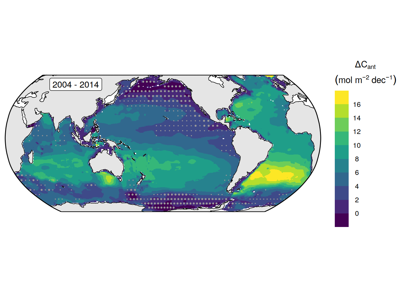
| Version | Author | Date |
|---|---|---|
| 8ded995 | jens-daniel-mueller | 2023-01-05 |
legend_title <- expression(atop(Delta * Delta * C["ant"],
                                (mol ~ m ^ {
                                  -2
                                } ~ dec ^ {
                                  -1
                                })))

p_dcant_inv_delta <-
  p_map_mdim_robinson(df = delta_dcant_inv,
                      df_uncertainty = dcant_inv_uncert_delta,
                      var = "dcant_offset",
                      breaks = c(-Inf, seq(-8, 8, 2), Inf),
                      legend_title = legend_title,
                      col = "divergent") +
  geom_label(aes(
    label = "Decadal difference",
    x = lon_lim[1] * 0.55,
    y = lat_lim[2] * 0.85
  ))


p_dcant_inv_delta
| Version | Author | Date |
|---|---|---|
| 8ded995 | jens-daniel-mueller | 2023-01-05 |
(p_dcant_inv_dec1 / p_dcant_inv_dec2 + plot_layout(guides = "collect")) -
  p_dcant_inv_delta +
  plot_layout(ncol = 1) +
  plot_annotation(tag_levels = 'A')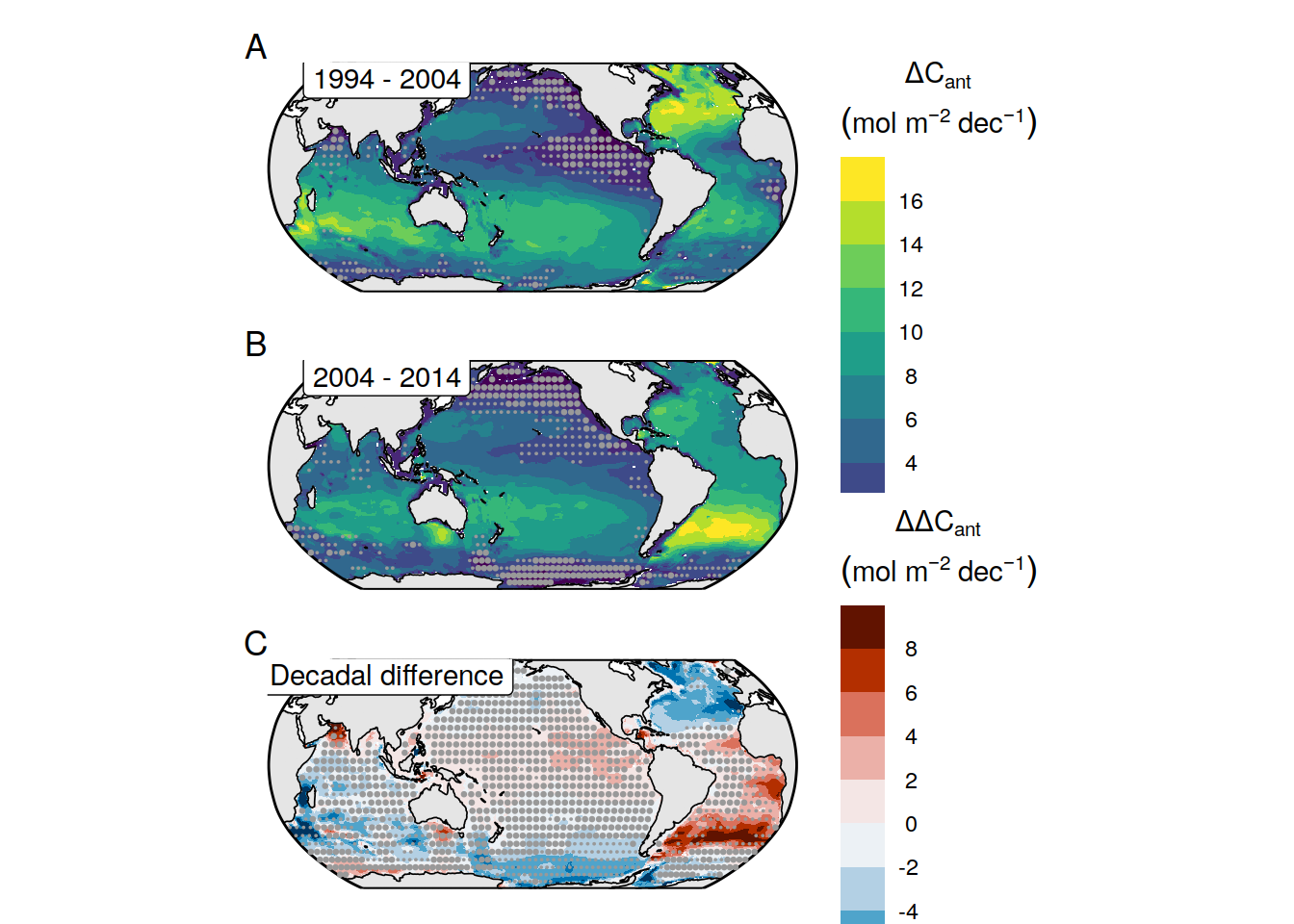
| Version | Author | Date |
|---|---|---|
| 8ded995 | jens-daniel-mueller | 2023-01-05 |
ggsave(path = here::here("output/publication"),
       filename = "Fig_dcant_column_inventory.png",
       height = 10,
       width = 8,
       dpi = 600)
legend_title <- expression(atop(Delta * C["ant"],
(mol ~ m ^ {
-2
} ~ dec ^ {
-1
})))
p_dcant_inv_dec1 <-
p_map_mdim_robinson(df = dcant_inv_dec1,
var = "dcant",
legend_title = legend_title) +
geom_label(aes(
label = "1994 - 2004",
x = lon_lim[1] * 0.55,
y = lat_lim[2] * 0.85
))
p_dcant_inv_dec2 <-
p_map_mdim_robinson(df = dcant_inv_dec2,
var = "dcant",
legend_title = legend_title) +
geom_label(aes(
label = "2004 - 2014",
x = lon_lim[1] * 0.55,
y = lat_lim[2] * 0.85
))
p_dcant_inv_dec1 / p_dcant_inv_dec2 +
plot_layout(guides = "collect") +
plot_layout(ncol = 1)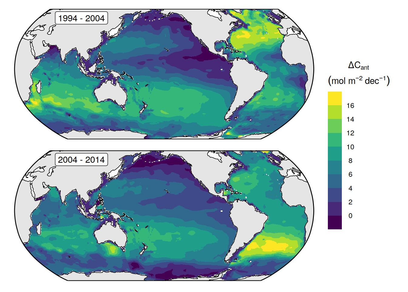
| Version | Author | Date |
|---|---|---|
| 2cca4eb | jens-daniel-mueller | 2023-01-10 |
ggsave(path = here::here("output/presentation"),
       filename = "Fig_dcant_column_inventory.png",
       height = 7,
       width = 8,
       dpi = 600)

p_dcant_inv_dec1 <-
  p_map_mdim_robinson(df = dcant_inv_dec1,
                      df_uncertainty = dcant_inv_uncert_dec1,
                      var = "dcant",
                      legend_title = legend_title) +
  geom_label(aes(
    label = "1994 - 2004",
    x = lon_lim[1] * 0.55,
    y = lat_lim[2] * 0.85
  ))


p_dcant_inv_dec1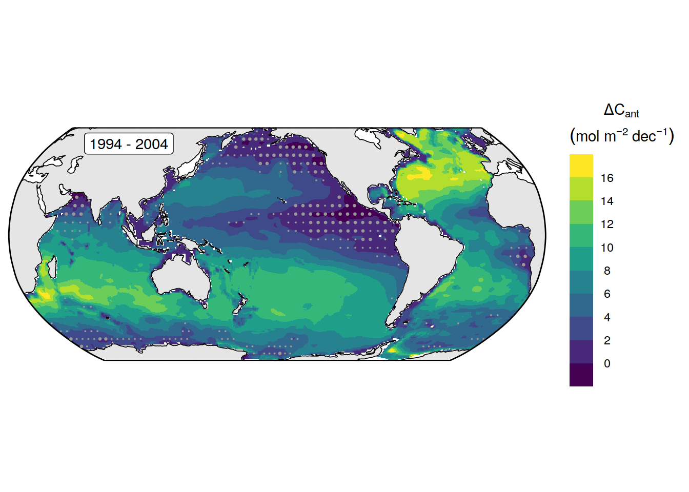
| Version | Author | Date |
|---|---|---|
| 2cca4eb | jens-daniel-mueller | 2023-01-10 |
p_dcant_inv_dec2 <-
  p_map_mdim_robinson(df = dcant_inv_dec2,
                      df_uncertainty = dcant_inv_uncert_dec2,
                      var = "dcant",
                      legend_title = legend_title) +
  geom_label(aes(
    label = "2004 - 2014",
    x = lon_lim[1] * 0.55,
    y = lat_lim[2] * 0.85
  ))


p_dcant_inv_dec2
| Version | Author | Date |
|---|---|---|
| 2cca4eb | jens-daniel-mueller | 2023-01-10 |
p_dcant_inv_dec1 / p_dcant_inv_dec2 +
  plot_layout(guides = "collect") +
  plot_layout(ncol = 1)
| Version | Author | Date |
|---|---|---|
| 2cca4eb | jens-daniel-mueller | 2023-01-10 |
ggsave(path = here::here("output/presentation"),
       filename = "Fig_dcant_column_inventory_uncertainty.png",
       height = 7,
       width = 8,
       dpi = 600)


legend_title <- expression(atop(Delta * Delta * C["ant"],
                                (mol ~ m ^ {
                                  -2
                                } ~ dec ^ {
                                  -1
                                })))

p_dcant_inv_delta <-
  p_map_mdim_robinson(df = delta_dcant_inv,
                      var = "dcant_offset",
                      breaks = c(-Inf, seq(-8, 8, 2), Inf),
                      legend_title = legend_title,
                      col = "divergent") +
  geom_label(aes(
    label = "Decadal difference",
    x = lon_lim[1] * 0.55,
    y = lat_lim[2] * 0.85
  ))


p_dcant_inv_delta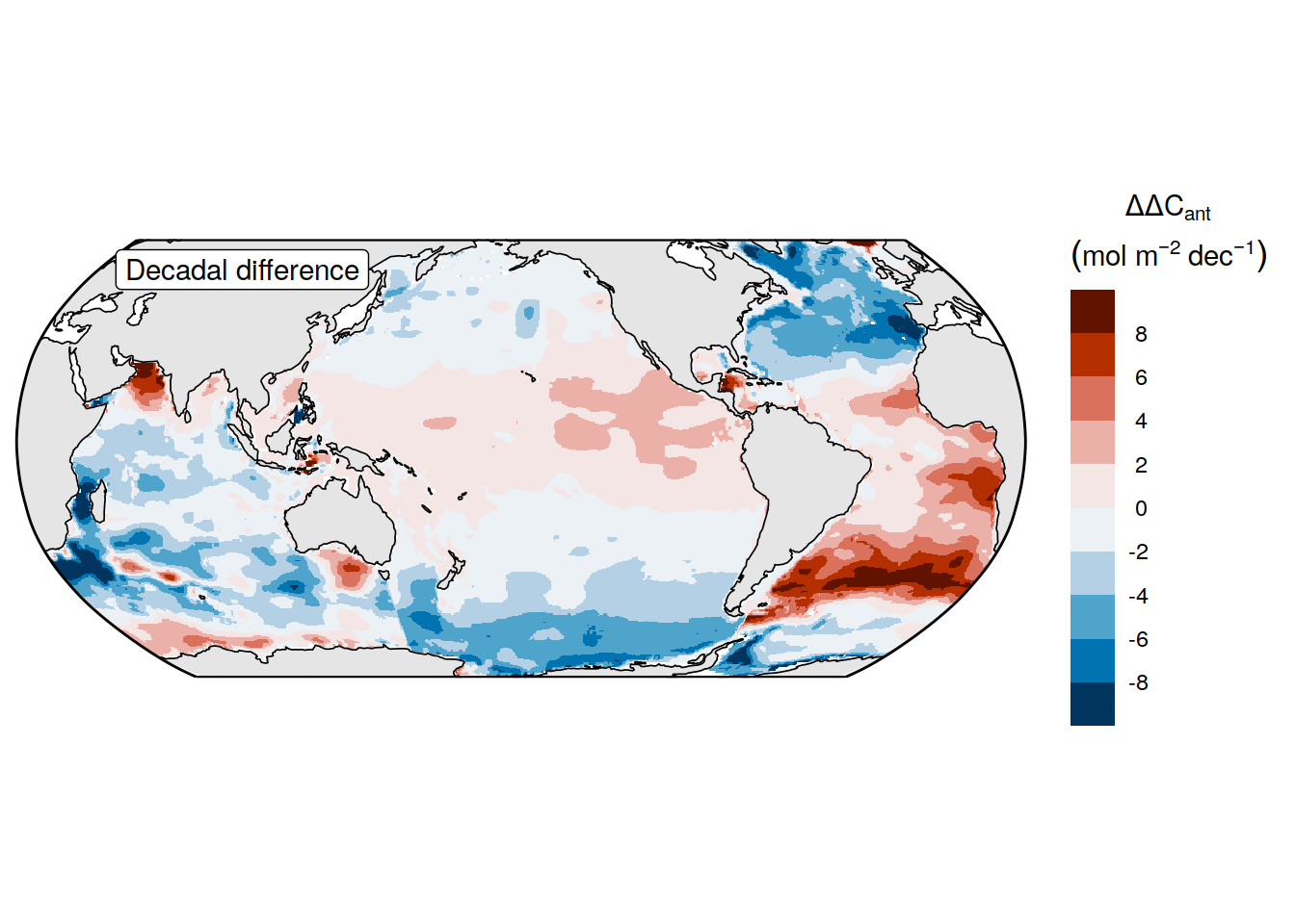
| Version | Author | Date |
|---|---|---|
| 2cca4eb | jens-daniel-mueller | 2023-01-10 |
ggsave(path = here::here("output/presentation"),
       filename = "Fig_delta_dcant_column_inventory.png",
       height = 4,
       width = 8,
       dpi = 600)

p_dcant_inv_delta <-
  p_map_mdim_robinson(df = delta_dcant_inv,
                      df_uncertainty = dcant_inv_uncert_delta,
                      var = "dcant_offset",
                      breaks = c(-Inf, seq(-8, 8, 2), Inf),
                      legend_title = legend_title,
                      col = "divergent") +
  geom_label(aes(
    label = "Decadal difference",
    x = lon_lim[1] * 0.55,
    y = lat_lim[2] * 0.85
  ))


p_dcant_inv_delta
| Version | Author | Date |
|---|---|---|
| 2cca4eb | jens-daniel-mueller | 2023-01-10 |
ggsave(path = here::here("output/presentation"),
       filename = "Fig_delta_dcant_column_inventory_uncertainty.png",
       height = 4,
       width = 8,
       dpi = 600)
9.6 Bias
dcant_inv_all %>%
  filter(period %in% two_decades,
         data_source != "obs") %>%
  mutate(
    data_source = case_when(
      data_source == "mod" ~ "Reconstruction",
      data_source == "mod_truth" ~ "Model truth"
    )
  ) %>%
  p_map_cant_inv(var = "dcant",
                 title_text = NULL) +
  facet_grid(data_source ~ period) +
  theme(axis.text.x = element_blank())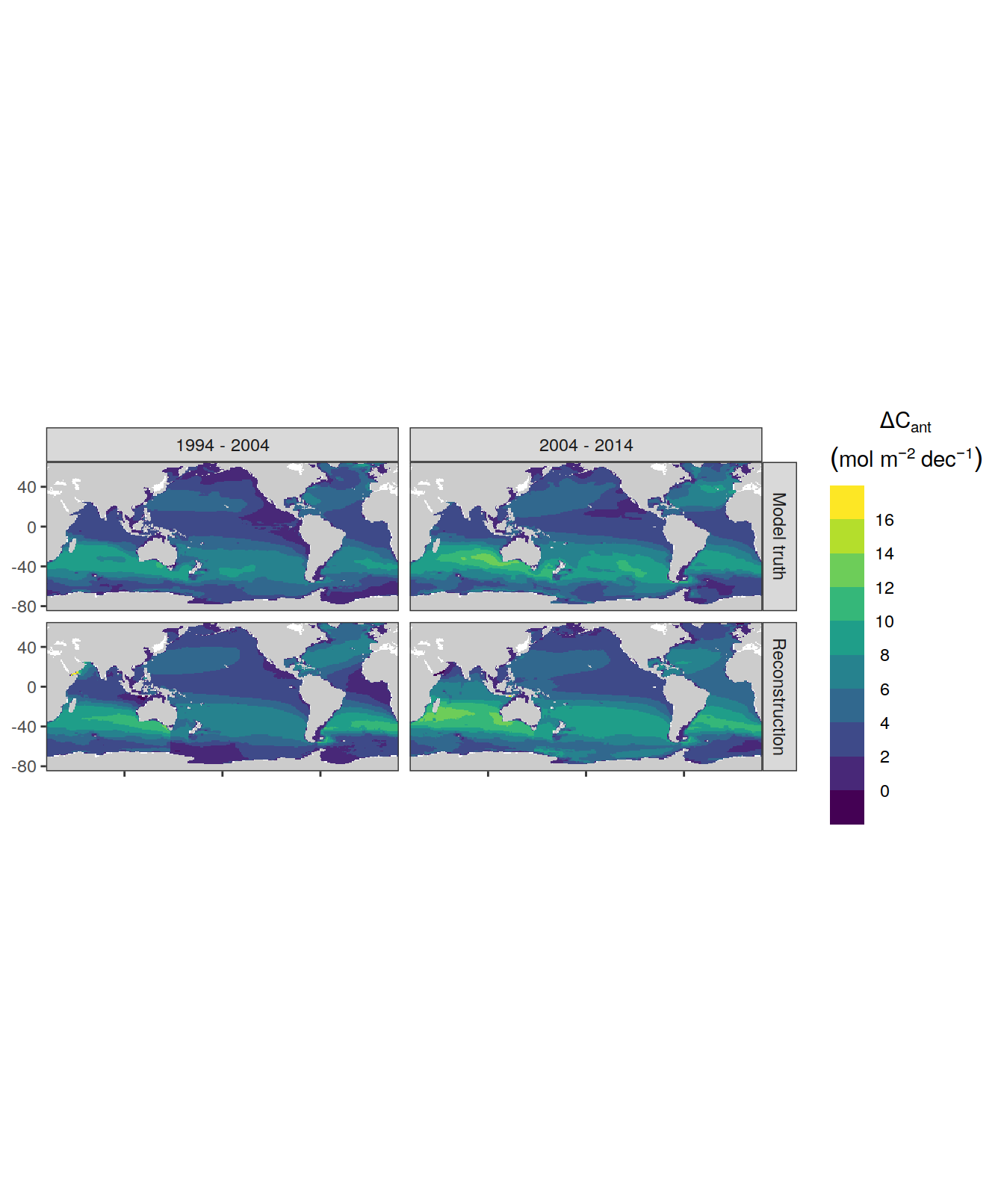
| Version | Author | Date |
|---|---|---|
| 8ded995 | jens-daniel-mueller | 2023-01-05 |
| 3a7bab0 | jens-daniel-mueller | 2022-11-28 |
| 322b1c1 | jens-daniel-mueller | 2022-11-25 |
| 491f8b1 | jens-daniel-mueller | 2022-11-25 |
| 4da4d66 | jens-daniel-mueller | 2022-11-25 |
| 534ee74 | jens-daniel-mueller | 2022-11-25 |
| 5520de8 | jens-daniel-mueller | 2022-11-15 |
| 1dad51a | jens-daniel-mueller | 2022-11-15 |
| 6edad9b | jens-daniel-mueller | 2022-11-11 |
| 16beb51 | jens-daniel-mueller | 2022-11-08 |
| b92657d | jens-daniel-mueller | 2022-11-08 |
| 7275091 | jens-daniel-mueller | 2022-11-05 |
legend_title <- expression(atop(Delta * C["ant"],
                                (mol ~ m ^ {
                                  -2
                                } ~ dec ^ {
                                  -1
                                })))

 p_CI_absolute_mod <- p_map_mdim_robinson(
  df = dcant_inv_all %>%
    filter(period %in% two_decades,
           data_source != "obs") %>%
    mutate(
      data_source = case_when(
        data_source == "mod" ~ "Reconstruction",
        data_source == "mod_truth" ~ "Model truth"
      )
    ) %>%
    select(lon, lat, period, data_source, dcant),
  dim_col = "period",
  dim_row = "data_source",
  var = "dcant",
  legend_title = legend_title
)


p_CI_absolute_mod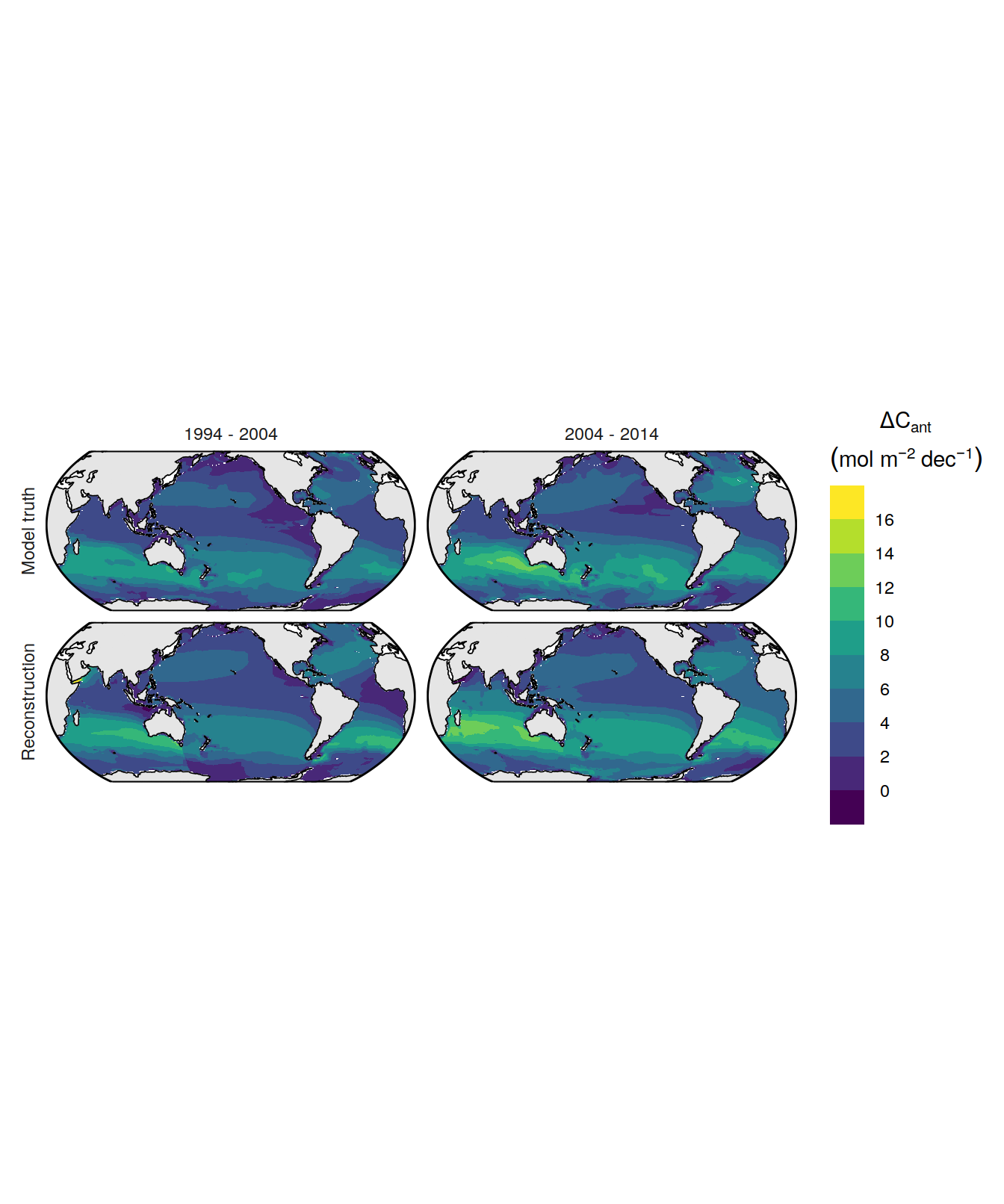
| Version | Author | Date |
|---|---|---|
| 8ded995 | jens-daniel-mueller | 2023-01-05 |
dcant_inv_all %>%
  filter(period %in% two_decades,
         data_source != "obs") %>%
  select(data_source, lon, lat, basin_AIP, period, dcant) %>%
  pivot_wider(names_from = data_source,
              values_from = dcant) %>%
  mutate(dcant_bias = mod - mod_truth,
         data_source = "Reconstruction bias") %>%
  p_map_cant_inv(
    var = "dcant_bias",
    title_text = NULL,
    subtitle_text = NULL,
    col = "bias"
  ) +
  facet_grid(data_source ~ period) +
  theme(strip.text.x = element_blank(),
        strip.background.x = element_blank())
| Version | Author | Date |
|---|---|---|
| 8ded995 | jens-daniel-mueller | 2023-01-05 |
| 3a7bab0 | jens-daniel-mueller | 2022-11-28 |
| 322b1c1 | jens-daniel-mueller | 2022-11-25 |
| 491f8b1 | jens-daniel-mueller | 2022-11-25 |
| 4da4d66 | jens-daniel-mueller | 2022-11-25 |
| 534ee74 | jens-daniel-mueller | 2022-11-25 |
| 5520de8 | jens-daniel-mueller | 2022-11-15 |
| 1dad51a | jens-daniel-mueller | 2022-11-15 |
| 6edad9b | jens-daniel-mueller | 2022-11-11 |
| 16beb51 | jens-daniel-mueller | 2022-11-08 |
| b92657d | jens-daniel-mueller | 2022-11-08 |
| 7275091 | jens-daniel-mueller | 2022-11-05 |
| 2345935 | jens-daniel-mueller | 2022-10-29 |
| 46c163a | jens-daniel-mueller | 2022-10-10 |
| 051b911 | jens-daniel-mueller | 2022-09-07 |
| 75bd58c | jens-daniel-mueller | 2022-09-07 |
| 1c6de0d | jens-daniel-mueller | 2022-09-07 |
| 78dbb27 | jens-daniel-mueller | 2022-08-11 |
| 302d289 | jens-daniel-mueller | 2022-08-11 |
| 5b77c4f | jens-daniel-mueller | 2022-08-10 |
legend_title <- expression(atop(Delta * C["ant"] ~ bias,
                                (mol ~ m ^ {
                                  -2
                                } ~ dec ^ {
                                  -1
                                })))

p_CI_bias <- p_map_mdim_robinson(
  df = dcant_inv_all %>%
    filter(period %in% two_decades,
           data_source != "obs") %>%
    select(data_source, lon, lat, basin_AIP, period, dcant) %>%
    pivot_wider(names_from = data_source,
                values_from = dcant) %>%
    mutate(dcant_bias = mod - mod_truth,
           data_source = "Reconstruction bias") %>%
    select(lon, lat, data_source, period, dcant_bias),
  dim_row = "data_source",
  dim_col = "period",
  var = "dcant_bias",
  breaks = c(-Inf, seq(-8, 8, 2), Inf),
  legend_title = legend_title,
  col = "divergent"
)

p_CI_absolute_mod / p_CI_bias +
  plot_annotation(tag_levels = 'A')
| Version | Author | Date |
|---|---|---|
| 8ded995 | jens-daniel-mueller | 2023-01-05 |
ggsave(path = here::here("output/publication"),
       filename = "FigS_dcant_column_inventory_synthetic_data.png",
       height = 7,
       width = 8,
       dpi = 600)

rm(p_CI_absolute_mod, p_CI_bias)

dcant_inv_all %>%
  filter(period %in% two_decades,
         data_source != "obs") %>%
  select(data_source, lon, lat, basin_AIP, period, dcant) %>%
  pivot_wider(names_from = data_source,
              values_from = dcant) %>%
  mutate(dcant_bias = mod - mod_truth,
         data_source = "Reconstruction bias") %>%
  mutate(area = earth_surf(lat,lon),
         dcant_bias_int = cut(abs(dcant_bias), c(-Inf,2,4,Inf))) %>%
  group_by(dcant_bias_int) %>%
  summarise(area = sum(area)) %>%
  ungroup() %>%
  mutate(area_fraction = 100 * area / sum(area))
# A tibble: 3 × 3
dcant_bias_int area area_fraction
<fct> <dbl> <dbl>
1 (-Inf,2] 5.74e14 87.1
2 (2,4] 8.23e13 12.5
3 (4, Inf] 2.54e12 0.385dcant_inv_all %>%
filter(period %in% two_decades,
data_source == "mod_truth") %>%
mutate(area = earth_surf(lat,lon),
dcant_int = cut(abs(dcant), c(-Inf,2,4,Inf))) %>%
group_by(dcant_int) %>%
summarise(area = sum(area)) %>%
ungroup() %>%
mutate(area_fraction = 100 * area / sum(area))# A tibble: 3 × 3
dcant_int area area_fraction
<fct> <dbl> <dbl>
1 (-Inf,2] 6.22e13 9.43
2 (2,4] 2.33e14 35.3
3 (4, Inf] 3.64e14 55.3 dcant_inv_all %>%
filter(period %in% two_decades,
data_source != "obs") %>%
select(data_source, lon, lat, basin_AIP, period, dcant) %>%
pivot_wider(names_from = data_source,
values_from = dcant) %>%
mutate(dcant_bias = mod - mod_truth,
data_source = "Reconstruction bias") %>%
arrange(period) %>%
group_by(lon, lat) %>%
summarise(delta_dcant_bias = dcant_bias - lag(dcant_bias)) %>%
ungroup() %>%
drop_na() %>%
p_map_cant_inv(
var = "delta_dcant_bias",
title_text = NULL,
subtitle_text = NULL,
col = "bias"
) +
theme(strip.text.x = element_blank(),
strip.background.x = element_blank())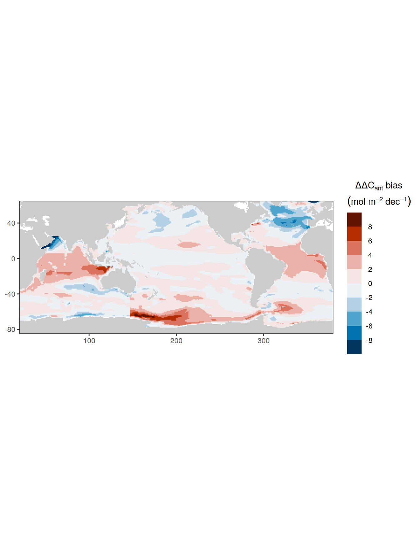
legend_title <- expression(atop(Delta * Delta * C["ant"] ~ bias,
                                (mol ~ m ^ {
                                  -2
                                } ~ dec ^ {
                                  -1
                                })))

p_CI_bias_decade <-
  p_map_mdim_robinson(
    df = dcant_inv_all %>%
      filter(period %in% two_decades,
             data_source != "obs") %>%
      select(data_source, lon, lat, basin_AIP, period, dcant) %>%
      pivot_wider(names_from = data_source,
                  values_from = dcant) %>%
      mutate(dcant_bias = mod - mod_truth,
             data_source = "Reconstruction bias") %>%
      arrange(period) %>%
      group_by(lon, lat) %>%
      summarise(delta_dcant_bias = dcant_bias - lag(dcant_bias)) %>%
      ungroup() %>%
      drop_na(),
    var = "delta_dcant_bias",
    breaks = c(-Inf, seq(-8, 8, 2), Inf),
    legend_title = legend_title,
    col = "divergent"
  )


p_CI_bias_decade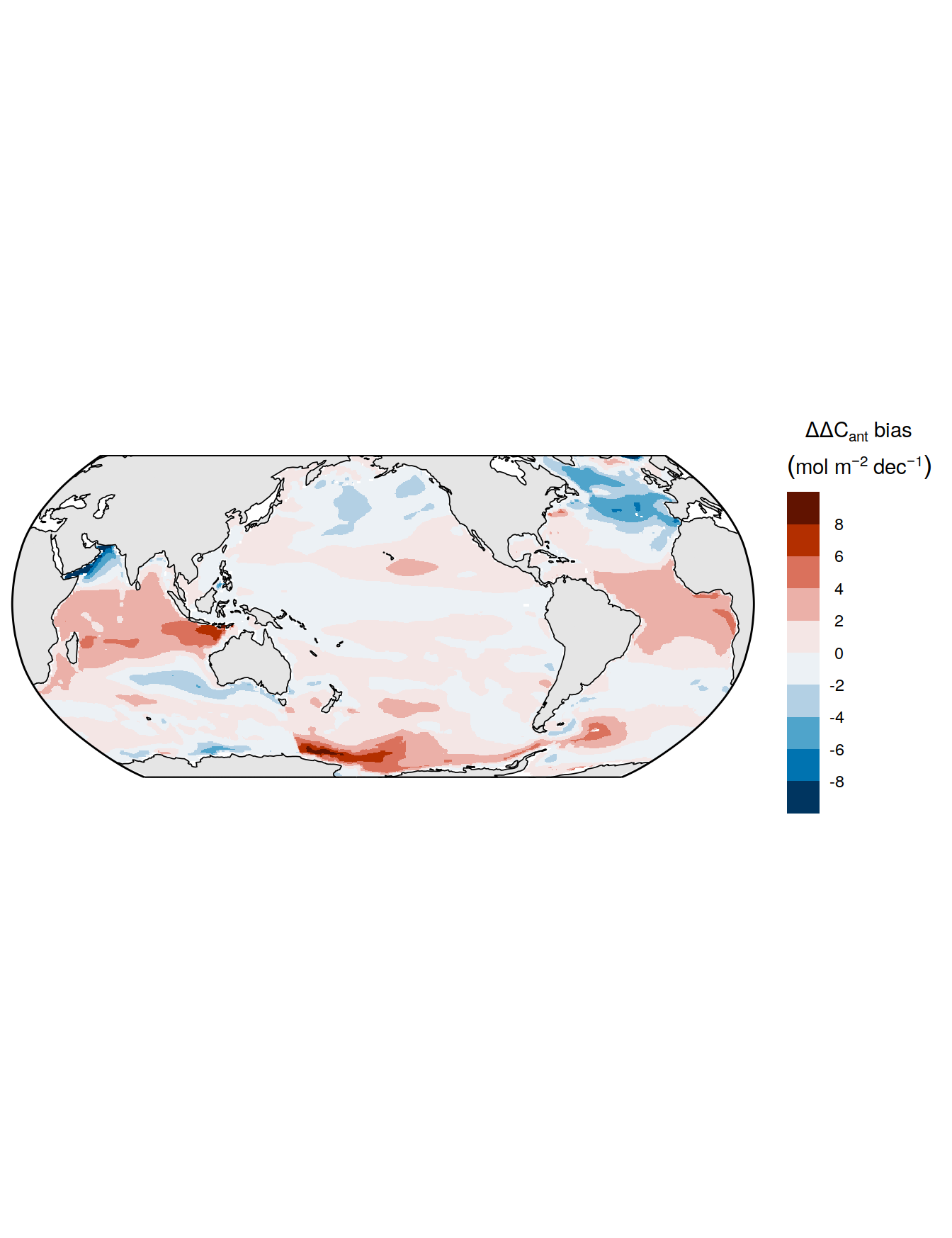
| Version | Author | Date |
|---|---|---|
| 8ded995 | jens-daniel-mueller | 2023-01-05 |
ggsave(path = here::here("output/publication"),
       filename = "FigS_delta_dcant_column_inventory_synthetic_data_bias.png",
       height = 3.5,
       width = 5,
       dpi = 600)

rm(p_CI_bias_decade)
9.7 Density distributions
bind_rows(
  dcant_inv_all %>%
    filter(period %in% two_decades) %>%
    mutate(
      data_source = case_when(
        data_source == "mod" ~ "Reconstruction",
        data_source == "obs" ~ "Observations",
        data_source == "mod_truth" ~ "Model truth"
      )
    ) %>%
    select(data_source, dcant, period),
  dcant_inv_bias_all %>%
    filter(period %in% two_decades) %>%
    mutate(data_source = "Reconstruction bias") %>%
    select(data_source, dcant = dcant_pos_bias, period)
) %>%
  ggplot(aes(dcant, col = data_source)) +
  scale_color_brewer(palette = "Dark2") +
  scale_fill_brewer(palette = "Dark2") +
  geom_vline(xintercept = 0) +
  geom_density(alpha = 0.3) +
  coord_cartesian(xlim = c(-2, 18)) +
  facet_grid(period ~ .) +
  labs(x = dcant_CI_label) +
  theme(legend.title = element_blank())
# ggsave(path = here::here("output/publication"),
#        filename = "FigS_dcant_column_inventory_density_distribution.png",
#        height = 4,
#        width = 7)
bind_rows(
dcant_inv_all %>%
filter(period %in% two_decades) %>%
select(data_source, lon, lat, period, dcant) %>%
pivot_wider(names_from = period,
values_from = dcant) %>%
mutate(dcant_offset = `2004 - 2014` - `1994 - 2004`,
period = "(2004 - 2014) - (1994 - 2004)") %>%
mutate(
data_source = case_when(
data_source == "mod" ~ "Reconstruction",
data_source == "obs" ~ "Observations",
data_source == "mod_truth" ~ "Model truth"
)
) %>%
select(data_source, dcant_offset, period),
dcant_inv_bias_all %>%
filter(period %in% two_decades) %>%
select(lon, lat, period, dcant_bias) %>%
pivot_wider(names_from = period,
values_from = dcant_bias) %>%
mutate(dcant_offset = `2004 - 2014` - `1994 - 2004`,
period = "(2004 - 2014) - (1994 - 2004)") %>%
mutate(data_source = "Reconstruction bias") %>%
select(data_source, dcant_offset, period)
) %>%
ggplot(aes(dcant_offset, col = data_source)) +
scale_color_brewer(palette = "Dark2") +
scale_fill_brewer(palette = "Dark2") +
geom_vline(xintercept = 0) +
geom_density(alpha = 0.3) +
coord_cartesian(xlim = c(-10, 10)) +
labs(x = delta_dcant_CI_label) +
theme(legend.title = element_blank())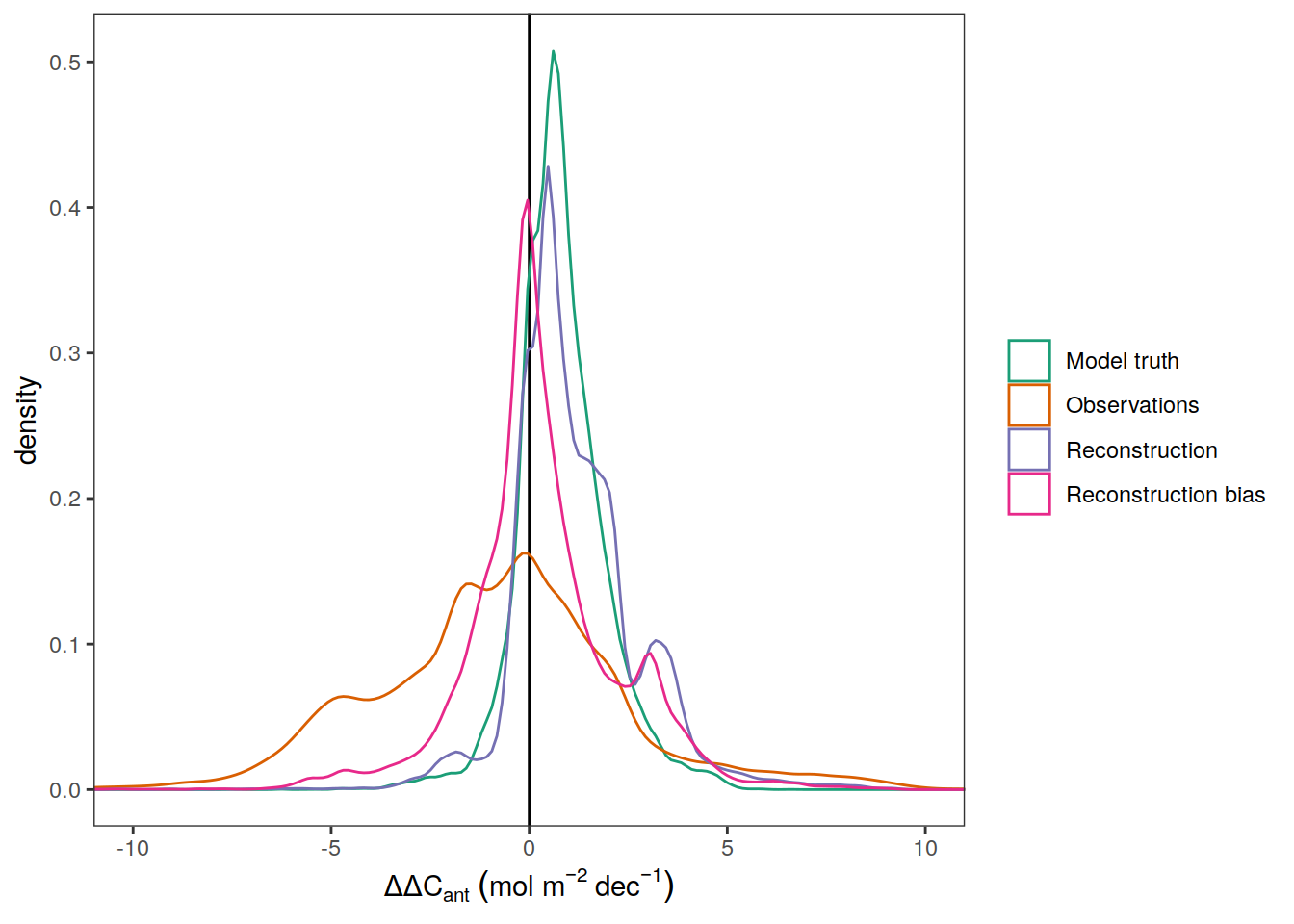
# ggsave(
#   path = here::here("output/publication"),
#   filename = "FigS_delta_dcant_column_inventory_density_distribution.png",
#   height = 3,
#   width = 7
# )
9.8 Beta
dcant_inv_all %>%
  filter(data_source %in% c("obs")) %>%
  p_map_cant_inv(var = "beta",
                 breaks = c(-Inf, seq(0, 1, 0.1), Inf),
                 title_text = NULL,
                 legend_title = beta_CI_label) +
  facet_wrap(~ period, ncol = 2)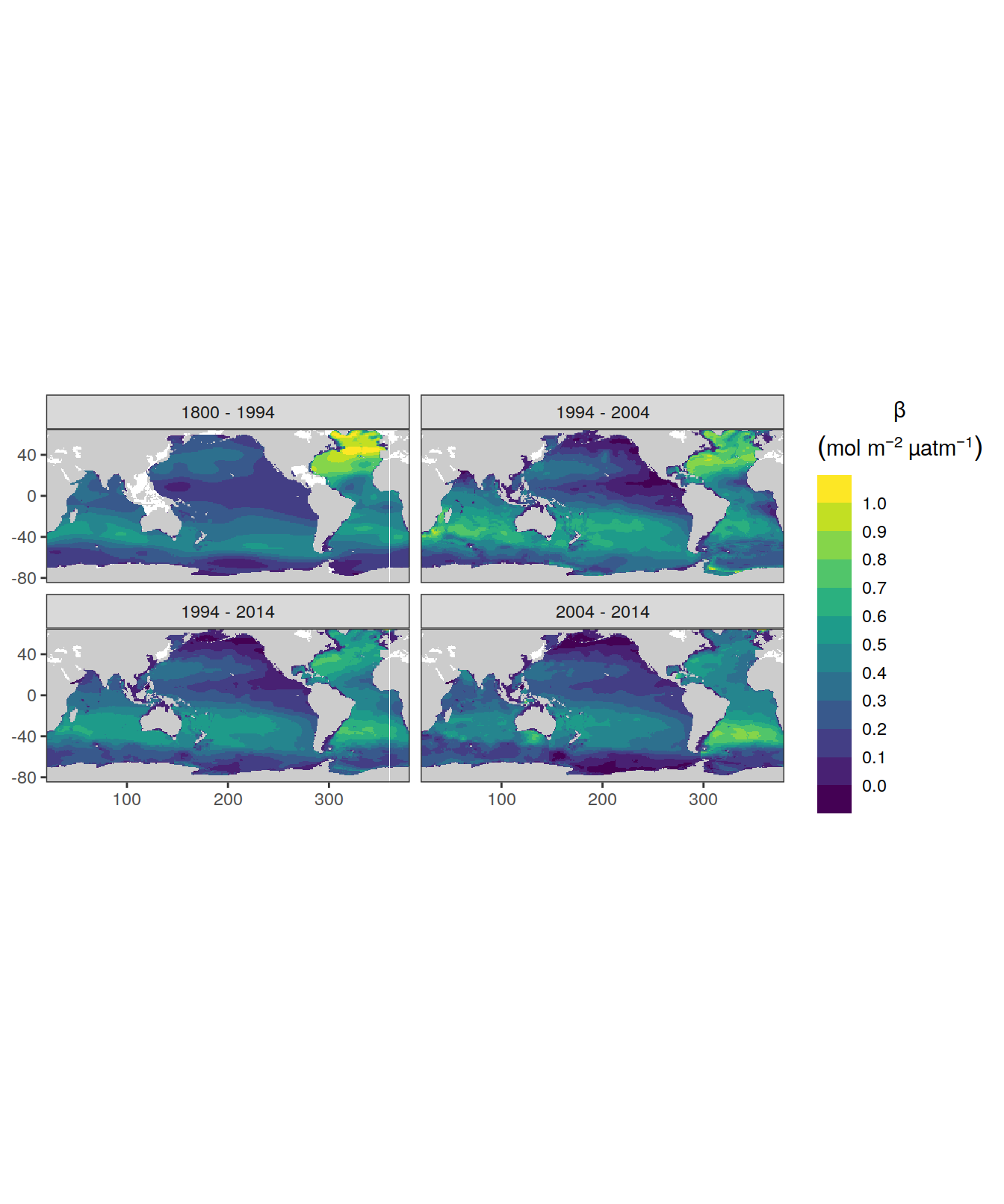
| Version | Author | Date |
|---|---|---|
| 3a7bab0 | jens-daniel-mueller | 2022-11-28 |
| e924c80 | jens-daniel-mueller | 2022-11-17 |
| 2345935 | jens-daniel-mueller | 2022-10-29 |
| 46c163a | jens-daniel-mueller | 2022-10-10 |
| 051b911 | jens-daniel-mueller | 2022-09-07 |
| 75bd58c | jens-daniel-mueller | 2022-09-07 |
| 1c6de0d | jens-daniel-mueller | 2022-09-07 |
| 78dbb27 | jens-daniel-mueller | 2022-08-11 |
| 302d289 | jens-daniel-mueller | 2022-08-11 |
| f68fcfa | jens-daniel-mueller | 2022-07-26 |
| f2615fb | jens-daniel-mueller | 2022-07-26 |
| fea41c1 | jens-daniel-mueller | 2022-07-20 |
| b1f7ab3 | jens-daniel-mueller | 2022-07-18 |
| d2ae54c | jens-daniel-mueller | 2022-07-18 |
| efa414b | jens-daniel-mueller | 2022-07-16 |
p_map_mdim_robinson(
  df = dcant_inv_all %>%
    filter(data_source %in% c("obs")) %>%
    select(lon, lat, period, beta),
  legend_title = beta_CI_label,
  var = "beta",
  breaks = c(-Inf, seq(0, 1, 0.1), Inf),
  dim_row = "period"
)
| Version | Author | Date |
|---|---|---|
| 8ded995 | jens-daniel-mueller | 2023-01-05 |
ggsave(path = here::here("output/publication"),
       filename = "FigS_beta_column_inventory.png",
       height = 10,
       width = 8,
       dpi = 600)
9.9 Zonal means
dcant_inv_all <- m_grid_horizontal_coarse(dcant_inv_all)

dcant_inv_all_lat_mean <- dcant_inv_all %>%
  group_by(basin_AIP, period, lat_grid, data_source) %>%
  summarise(beta = mean(beta, na.rm = TRUE),
            dcant = mean(dcant, na.rm = TRUE)) %>%
  ungroup()

dcant_inv_all_ensemble <- m_grid_horizontal_coarse(dcant_inv_all_ensemble)

dcant_inv_all_ensemble_lat_mean <- dcant_inv_all_ensemble %>%
  group_by(basin_AIP, period, lat_grid, Version_ID, data_source) %>%
  summarise(beta_mean = mean(beta, na.rm = TRUE),
            dcant_mean = mean(dcant, na.rm = TRUE)) %>%
  ungroup()

dcant_inv_all_ensemble_lat_mean_average <- dcant_inv_all_ensemble_lat_mean %>%
  group_by(basin_AIP, period, lat_grid, data_source) %>%
  summarise(beta_sd = sd(beta_mean, na.rm = TRUE),
            beta_mean = mean(beta_mean, na.rm = TRUE),
            dcant_sd = sd(dcant_mean, na.rm = TRUE),
            dcant_mean = mean(dcant_mean, na.rm = TRUE)) %>%
  ungroup()

dcant_inv_all_lat_mean <- full_join(dcant_inv_all_lat_mean,
                                    dcant_inv_all_ensemble_lat_mean_average)
9.9.1 dcant
dcant_inv_all_lat_mean %>%
  filter(period != "1800 - 1994") %>%
  ggplot(aes(lat_grid, dcant, fill = period)) +
  geom_hline(yintercept = c(0,10)) +
  geom_vline(xintercept = c(-10,10)) +
  geom_vline(xintercept = c(-40,-30,30,40)) +
  geom_ribbon(aes(ymin = dcant - dcant_sd,
                  ymax = dcant + dcant_sd),
              alpha = 0.3) +
  geom_path(aes(col = period)) +
  geom_point(shape = 21) +
  scale_color_brewer(palette = "Dark2", name = "Mean ± SD") +
  scale_fill_brewer(palette = "Dark2", name = "Mean ± SD") +
  coord_flip() +
  facet_grid(data_source ~ basin_AIP) +
  labs(x = "Latitude (°N)",
       y = dcant_CI_label) +
  scale_x_continuous(breaks = seq(-75,75, 15))
| Version | Author | Date |
|---|---|---|
| 3a7bab0 | jens-daniel-mueller | 2022-11-28 |
| 534ee74 | jens-daniel-mueller | 2022-11-25 |
| 5520de8 | jens-daniel-mueller | 2022-11-15 |
| 1dad51a | jens-daniel-mueller | 2022-11-15 |
| 6edad9b | jens-daniel-mueller | 2022-11-11 |
| 16beb51 | jens-daniel-mueller | 2022-11-08 |
| b92657d | jens-daniel-mueller | 2022-11-08 |
| 7275091 | jens-daniel-mueller | 2022-11-05 |
| 99610ed | jens-daniel-mueller | 2022-11-01 |
| 7060801 | jens-daniel-mueller | 2022-10-31 |
| ecb84c1 | jens-daniel-mueller | 2022-10-30 |
| 2345935 | jens-daniel-mueller | 2022-10-29 |
| 051b911 | jens-daniel-mueller | 2022-09-07 |
| 75bd58c | jens-daniel-mueller | 2022-09-07 |
| 1c6de0d | jens-daniel-mueller | 2022-09-07 |
| 78dbb27 | jens-daniel-mueller | 2022-08-11 |
| 302d289 | jens-daniel-mueller | 2022-08-11 |
| 5b77c4f | jens-daniel-mueller | 2022-08-10 |
| fea41c1 | jens-daniel-mueller | 2022-07-20 |
| d2ae54c | jens-daniel-mueller | 2022-07-18 |
| 2695085 | jens-daniel-mueller | 2022-07-17 |
| 535196a | jens-daniel-mueller | 2022-07-17 |
| afb27ad | jens-daniel-mueller | 2022-07-15 |
| b492b46 | jens-daniel-mueller | 2022-07-15 |
| bd24a0f | jens-daniel-mueller | 2022-07-15 |
| ea46812 | jens-daniel-mueller | 2022-07-13 |
dcant_inv_all_lat_mean %>%
  filter(period != "1800 - 1994") %>%
  mutate(lat_grid = cut(lat_grid, c(-40,-30,-10,10,30,40))) %>%
  group_by(lat_grid, data_source) %>%
  summarise(dcant_mean = mean(dcant_mean, na_rm = TRUE)) %>%
  ungroup()
# A tibble: 18 × 3
lat_grid data_source dcant_mean
<fct> <chr> <dbl>
1 (-40,-30] mod 11.7
2 (-40,-30] mod_truth 10.9
3 (-40,-30] obs 13.9
4 (-30,-10] mod 8.65
5 (-30,-10] mod_truth 7.73
6 (-30,-10] obs 11.1
7 (-10,10] mod 4.60
8 (-10,10] mod_truth 4.09
9 (-10,10] obs 6.87
10 (10,30] mod 5.31
11 (10,30] mod_truth 5.03
12 (10,30] obs 6.78
13 (30,40] mod 6.23
14 (30,40] mod_truth 6.46
15 (30,40] obs 10.6
16 <NA> mod 5.61
17 <NA> mod_truth 5.59
18 <NA> obs 7.08dcant_inv_all_lat_mean %>%
filter(period != "1800 - 1994") %>%
mutate(lat_grid = cut(lat_grid, c(-40,-30,-10,10,30,40))) %>%
group_by(lat_grid, basin_AIP, data_source) %>%
summarise(dcant_mean = mean(dcant_mean, na_rm = TRUE)) %>%
ungroup()# A tibble: 51 × 4
lat_grid basin_AIP data_source dcant_mean
<fct> <chr> <chr> <dbl>
1 (-40,-30] Atlantic mod 11.3
2 (-40,-30] Atlantic mod_truth 10.1
3 (-40,-30] Atlantic obs 15.1
4 (-40,-30] Indian mod 13.3
5 (-40,-30] Indian mod_truth 12.6
6 (-40,-30] Indian obs 13.8
7 (-40,-30] Pacific mod 10.5
8 (-40,-30] Pacific mod_truth 9.97
9 (-40,-30] Pacific obs 12.8
10 (-30,-10] Atlantic mod 7.55
# … with 41 more rowsdcant_inv_all_lat_mean %>%
filter(period != "1800 - 1994") %>%
mutate(lat_grid = cut(lat_grid, c(-90,0,90))) %>%
group_by(lat_grid, basin_AIP, period, data_source) %>%
summarise(dcant_mean = mean(dcant_mean, na_rm = TRUE)) %>%
ungroup()# A tibble: 54 × 5
lat_grid basin_AIP period data_source dcant_mean
<fct> <chr> <chr> <chr> <dbl>
1 (-90,0] Atlantic 1994 - 2004 mod 4.19
2 (-90,0] Atlantic 1994 - 2004 mod_truth 4.06
3 (-90,0] Atlantic 1994 - 2004 obs 6.68
4 (-90,0] Atlantic 1994 - 2014 mod 9.50
5 (-90,0] Atlantic 1994 - 2014 mod_truth 8.72
6 (-90,0] Atlantic 1994 - 2014 obs 14.4
7 (-90,0] Atlantic 2004 - 2014 mod 5.35
8 (-90,0] Atlantic 2004 - 2014 mod_truth 4.66
9 (-90,0] Atlantic 2004 - 2014 obs 7.77
10 (-90,0] Indian 1994 - 2004 mod 5.77
# … with 44 more rowsdcant_inv_all_lat_mean %>%
filter(period %in%two_decades,
data_source == "obs") %>%
mutate(lat_grid = cut(lat_grid, c(-50,-20,20,50))) %>%
group_by(lat_grid, basin_AIP, period, data_source) %>%
summarise(dcant_mean = mean(dcant_mean, na_rm = TRUE)) %>%
ungroup() %>%
filter(data_source == "obs") %>%
arrange(basin_AIP)# A tibble: 24 × 5
lat_grid basin_AIP period data_source dcant_mean
<fct> <chr> <chr> <chr> <dbl>
1 (-50,-20] Atlantic 1994 - 2004 obs 8.55
2 (-50,-20] Atlantic 2004 - 2014 obs 11.4
3 (-20,20] Atlantic 1994 - 2004 obs 5.23
4 (-20,20] Atlantic 2004 - 2014 obs 8.50
5 (20,50] Atlantic 1994 - 2004 obs 12.0
6 (20,50] Atlantic 2004 - 2014 obs 8.07
7 <NA> Atlantic 1994 - 2004 obs 7.39
8 <NA> Atlantic 2004 - 2014 obs 4.07
9 (-50,-20] Indian 1994 - 2004 obs 10.8
10 (-50,-20] Indian 2004 - 2014 obs 8.43
# … with 14 more rowsdcant_inv_all_ensemble_lat_mean %>%
ggplot(aes(lat_grid, dcant_mean, fill=period, group=Version_ID)) +
geom_hline(yintercept = 0) +
geom_path(aes(col=period), alpha = 0.3) +
scale_color_brewer(palette = "Dark2") +
scale_fill_brewer(palette = "Dark2") +
coord_flip() +
facet_grid(data_source ~ basin_AIP) +
labs(x = "Latitude (°N)",
y = dcant_CI_label)
| Version | Author | Date |
|---|---|---|
| 3a7bab0 | jens-daniel-mueller | 2022-11-28 |
| 534ee74 | jens-daniel-mueller | 2022-11-25 |
| 5520de8 | jens-daniel-mueller | 2022-11-15 |
| 1dad51a | jens-daniel-mueller | 2022-11-15 |
| 6edad9b | jens-daniel-mueller | 2022-11-11 |
| 16beb51 | jens-daniel-mueller | 2022-11-08 |
| b92657d | jens-daniel-mueller | 2022-11-08 |
| 7275091 | jens-daniel-mueller | 2022-11-05 |
| 99610ed | jens-daniel-mueller | 2022-11-01 |
| 7060801 | jens-daniel-mueller | 2022-10-31 |
| ecb84c1 | jens-daniel-mueller | 2022-10-30 |
| 2345935 | jens-daniel-mueller | 2022-10-29 |
| 051b911 | jens-daniel-mueller | 2022-09-07 |
| 75bd58c | jens-daniel-mueller | 2022-09-07 |
| 1c6de0d | jens-daniel-mueller | 2022-09-07 |
| 5b77c4f | jens-daniel-mueller | 2022-08-10 |
| fea41c1 | jens-daniel-mueller | 2022-07-20 |
| d2ae54c | jens-daniel-mueller | 2022-07-18 |
| 2695085 | jens-daniel-mueller | 2022-07-17 |
| 535196a | jens-daniel-mueller | 2022-07-17 |
| 0160c40 | jens-daniel-mueller | 2022-07-16 |
| afb27ad | jens-daniel-mueller | 2022-07-15 |
| b492b46 | jens-daniel-mueller | 2022-07-15 |
| bd24a0f | jens-daniel-mueller | 2022-07-15 |
| ea46812 | jens-daniel-mueller | 2022-07-13 |
9.9.2 beta
dcant_inv_all_lat_mean %>%
  ggplot(aes(lat_grid, beta, fill = period)) +
  geom_hline(yintercept = 0) +
  geom_ribbon(aes(ymin = beta - beta_sd,
                  ymax = beta + beta_sd),
              alpha = 0.3) +
  geom_path(aes(col = period)) +
  geom_point(shape = 21) +
  scale_color_brewer(palette = "Dark2", name = "Mean ± SD") +
  scale_fill_brewer(palette = "Dark2", name = "Mean ± SD") +
  coord_flip() +
  facet_grid(data_source ~ basin_AIP) +
  labs(x = "Latitude (°N)",
       y = beta_CI_label) +
  scale_x_continuous(breaks = seq(-75,75, 15))
| Version | Author | Date |
|---|---|---|
| 3a7bab0 | jens-daniel-mueller | 2022-11-28 |
| 534ee74 | jens-daniel-mueller | 2022-11-25 |
| 1dad51a | jens-daniel-mueller | 2022-11-15 |
| 6edad9b | jens-daniel-mueller | 2022-11-11 |
| 16beb51 | jens-daniel-mueller | 2022-11-08 |
| b92657d | jens-daniel-mueller | 2022-11-08 |
| 7275091 | jens-daniel-mueller | 2022-11-05 |
| 99610ed | jens-daniel-mueller | 2022-11-01 |
| 7060801 | jens-daniel-mueller | 2022-10-31 |
| ecb84c1 | jens-daniel-mueller | 2022-10-30 |
| 2345935 | jens-daniel-mueller | 2022-10-29 |
| 46c163a | jens-daniel-mueller | 2022-10-10 |
| 051b911 | jens-daniel-mueller | 2022-09-07 |
| 75bd58c | jens-daniel-mueller | 2022-09-07 |
| 1c6de0d | jens-daniel-mueller | 2022-09-07 |
| 78dbb27 | jens-daniel-mueller | 2022-08-11 |
| 302d289 | jens-daniel-mueller | 2022-08-11 |
| 5b77c4f | jens-daniel-mueller | 2022-08-10 |
| fea41c1 | jens-daniel-mueller | 2022-07-20 |
| d2ae54c | jens-daniel-mueller | 2022-07-18 |
| 2695085 | jens-daniel-mueller | 2022-07-17 |
| 535196a | jens-daniel-mueller | 2022-07-17 |
| afb27ad | jens-daniel-mueller | 2022-07-15 |
| b492b46 | jens-daniel-mueller | 2022-07-15 |
| bd24a0f | jens-daniel-mueller | 2022-07-15 |
| ea46812 | jens-daniel-mueller | 2022-07-13 |
dcant_inv_all_ensemble_lat_mean %>%
  ggplot(aes(lat_grid, beta_mean, fill=period, group=Version_ID)) +
  geom_hline(yintercept = 0) +
  geom_path(aes(col=period), alpha = 0.3) +
  scale_color_brewer(palette = "Dark2") +
  scale_fill_brewer(palette = "Dark2") +
  coord_flip() +
  facet_grid(data_source ~ basin_AIP) +
  labs(x = "Latitude (°N)",
       y = beta_CI_label)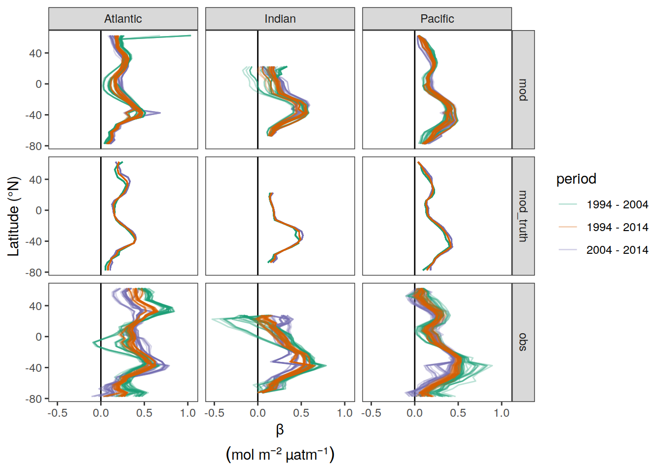
| Version | Author | Date |
|---|---|---|
| 3a7bab0 | jens-daniel-mueller | 2022-11-28 |
| 534ee74 | jens-daniel-mueller | 2022-11-25 |
| 1dad51a | jens-daniel-mueller | 2022-11-15 |
| 6edad9b | jens-daniel-mueller | 2022-11-11 |
| 16beb51 | jens-daniel-mueller | 2022-11-08 |
| b92657d | jens-daniel-mueller | 2022-11-08 |
| 7275091 | jens-daniel-mueller | 2022-11-05 |
| 99610ed | jens-daniel-mueller | 2022-11-01 |
| 7060801 | jens-daniel-mueller | 2022-10-31 |
| ecb84c1 | jens-daniel-mueller | 2022-10-30 |
| 2345935 | jens-daniel-mueller | 2022-10-29 |
| 46c163a | jens-daniel-mueller | 2022-10-10 |
| 051b911 | jens-daniel-mueller | 2022-09-07 |
| 75bd58c | jens-daniel-mueller | 2022-09-07 |
| 1c6de0d | jens-daniel-mueller | 2022-09-07 |
| 5b77c4f | jens-daniel-mueller | 2022-08-10 |
| fea41c1 | jens-daniel-mueller | 2022-07-20 |
| d2ae54c | jens-daniel-mueller | 2022-07-18 |
| 2695085 | jens-daniel-mueller | 2022-07-17 |
| 535196a | jens-daniel-mueller | 2022-07-17 |
| 0160c40 | jens-daniel-mueller | 2022-07-16 |
| afb27ad | jens-daniel-mueller | 2022-07-15 |
| b492b46 | jens-daniel-mueller | 2022-07-15 |
| bd24a0f | jens-daniel-mueller | 2022-07-15 |
| ea46812 | jens-daniel-mueller | 2022-07-13 |
9.10 Write files
dcant_inv_out <- dcant_inv_all_ensemble %>%
  filter(
    period %in% two_decades &
      data_source == "obs" &
      (MLR_basins == "3" |
         Version_ID_group == "Standard case")
  )

Version_IDs_out <- dcant_inv_out %>%
  distinct(Version_ID, period, Version_ID_group, MLR_basins)

dcant_inv_out <- dcant_inv_out %>%
  select(lon,
         lat,
         period,
         MLR_basins,
         Version_ID_group,
         dcant)

# convert from tibble to stars object
dcant_inv_out_stars <- st_as_stars(dcant_inv_out,
                                   dims = c("lon", "lat", "period", "MLR_basins", "Version_ID_group"))

# assign coordinate system to horizontal (lon, lat) coordinates
# st_crs(dcant_inv_out_stars) <- "+proj=longlat"
st_crs(dcant_inv_out_stars) <- st_crs(4326)

# plot variable per depth level
ggplot() +
  geom_stars(data = dcant_inv_out_stars %>%
               filter(period == "1994 - 2004")) +
  facet_grid(MLR_basins~Version_ID_group) +
  scale_fill_viridis_b(breaks = c(-Inf, seq(0,16,2), Inf),
                       na.value = "transparent")

file_out <- paste0(path_out, "inv_dcant_emlr_cstar_mueller_94-04-14.nc")

# write stars object to .nc file
dcant_inv_out_stars %>%
  write_mdim(file_out)


# reopen .nc file with all available stars functions
dcant_inv_read_ncdf <-
  read_ncdf(file_out)
dcant_inv_read_mdim <-
  read_mdim(file_out)

# plot variable in object reopened

ggplot() +
  geom_stars(data = dcant_inv_read_ncdf %>%
               filter(period == "1994 - 2004")) +
  facet_grid(MLR_basins~Version_ID_group) +
  scale_fill_viridis_b(breaks = c(-Inf, seq(0,16,2), Inf),
                       na.value = "transparent")

ggplot() +
  geom_stars(data = dcant_inv_read_mdim %>%
               filter(period == "1994 - 2004")) +
  facet_grid(MLR_basins~Version_ID_group) +
  scale_fill_viridis_b(breaks = c(-Inf, seq(0,16,2), Inf),
                       na.value = "transparent")

ggplot() +
  geom_stars(data = dcant_inv_read_ncdf %>%
               filter(MLR_basins == "3")) +
  facet_grid(period~Version_ID_group) +
  scale_fill_viridis_b(breaks = c(-Inf, seq(0,16,2), Inf),
                       na.value = "transparent") +
  coord_quickmap()


dcant_inv_read_tidync <-
  tidync::tidync(file_out)

dcant_inv_read_tidync %>%
  tidync::hyper_tibble() %>%
  filter(period == "1994 - 2004") %>%
  ggplot(aes(lon, lat, fill = dcant)) +
  geom_raster() +
  facet_grid(MLR_basins ~ Version_ID_group) +
  scale_fill_viridis_b(breaks = c(-Inf, seq(0,16,2), Inf),
                       na.value = "transparent")

# library(ncdf4)
#
# nc <- nc_open(file_out)
# print(nc)
#
# # get longitude and latitude
# lon <- ncvar_get(nc,"period")
# nlon <- dim(lon)
#
#
# ncatt_get(nc, "period")
# ncvar_get(nc)
#
# nt <- dim(time)
#
# nc_close(nc)
delta_dcant_inv_uncertainty_out <- delta_dcant_inv_uncertainty %>%
filter(data_source == "obs") %>%
mutate(period = "decadal difference") %>%
select(lon, lat, period, dcant = delta_dcant, uncertainty = RSS)
dcant_inv_uncertainty_out <- dcant_inv_uncertainty %>%
filter(data_source == "obs") %>%
select(lon, lat, period, dcant = std_case, uncertainty = sd)
dcant_inv_uncertainty_out <- bind_rows(dcant_inv_uncertainty_out,
delta_dcant_inv_uncertainty_out)
# convert from tibble to stars object
dcant_inv_uncertainty_out_stars <- st_as_stars(
dcant_inv_uncertainty_out,
dims = c("lon", "lat", "period"))
# assign coordinate system to horizontal (lon, lat) coordinates
# st_crs(dcant_inv_out_stars) <- "+proj=longlat"
st_crs(dcant_inv_uncertainty_out_stars) <- st_crs(4326)
# plot variable per depth level
ggplot() +
geom_stars(data = dcant_inv_uncertainty_out_stars) +
facet_grid(period ~ .) +
scale_fill_binned_divergingx(
breaks = c(-Inf, seq(-16, 16, 4), Inf),
palette = "RdBu",
rev = TRUE,
na.value = "transparent"
)
ggplot() +
geom_stars(data = dcant_inv_uncertainty_out_stars,
aes(fill = abs(dcant) - uncertainty)) +
facet_grid(period ~ .) +
scale_fill_binned_divergingx(
breaks = c(-Inf, 0 , Inf),
palette = "RdBu",
rev = TRUE,
na.value = "transparent"
)
file_out <- paste0(path_out,"inv_dcant_emlr_cstar_mueller_94-04-14_uncertainty.nc")
# write stars object to .nc file
dcant_inv_uncertainty_out_stars %>%
write_mdim(file_out)
# reopen .nc file with all available stars functions
dcant_inv_uncertainty_read_ncdf <-
read_ncdf(file_out)
dcant_inv_uncertainty_read_mdim <-
read_mdim(file_out)
# plot variable in object reopened
ggplot() +
geom_stars(data = dcant_inv_uncertainty_read_ncdf,
aes(fill = abs(dcant) - uncertainty)) +
facet_grid(period ~ .) +
scale_fill_binned_divergingx(
breaks = c(-Inf, 0 , Inf),
palette = "RdBu",
rev = TRUE,
na.value = "transparent"
)
ggplot() +
geom_stars(data = dcant_inv_uncertainty_read_mdim,
aes(fill = abs(dcant) - uncertainty)) +
facet_grid(period ~ .) +
scale_fill_binned_divergingx(
breaks = c(-Inf, 0 , Inf),
palette = "RdBu",
rev = TRUE,
na.value = "transparent"
)
dcant_inv_uncertainty_read_tidync <-
tidync::tidync(file_out)
dcant_inv_uncertainty_read_tidync %>%
tidync::hyper_tibble() %>%
ggplot(aes(lon, lat)) +
geom_raster(aes(fill = abs(dcant) - uncertainty)) +
facet_grid(period ~ .) +
scale_fill_binned_divergingx(
breaks = c(-Inf, 0 , Inf),
palette = "RdBu",
rev = TRUE,
na.value = "transparent"
)
# library(ncdf4)
# nc_open(file_out)
# nc_close(file_out)10 Global section
10.1 Additive uncertainty
delta_dcant_global_section_all <-
  dcant_global_section_all %>%
  filter(data_source %in% c("obs", "mod"),
         period %in% two_decades) %>%
  select(data_source, dist, depth, period, dcant) %>%
  drop_na() %>%
  pivot_wider(names_from = period,
              values_from = dcant) %>%
  mutate(dcant_offset = `2004 - 2014` - `1994 - 2004`,
         period = "(2004 - 2014) - (1994 - 2004)")

dcant_global_section_all_uncertainty <-
  dcant_global_section_all_ensemble %>%
  filter(data_source %in% c("obs", "mod"),
         period %in% two_decades) %>%
  select(dist,
         depth,
         period,
         data_source,
         MLR_basins,
         Version_ID_group,
         dcant) %>%
  mutate(dist_grid = as.numeric(as.character(cut(
    dist, seq(0, 50, 1), seq(0.5, 49.5, 1)
  ))),
  # depth_grid = depth
  depth_grid = as.numeric(as.character(cut(
    depth,
    c(seq(0, 500, 100), seq(1000, 10000, 500)),
    c(seq(50, 450, 100), seq(750, 10000, 500)),
    right = FALSE
  )))
  ) %>%
  group_by(dist_grid,
           depth_grid,
           data_source,
           period,
           MLR_basins,
           Version_ID_group) %>%
  summarise(dcant = mean(dcant)) %>%
  ungroup() %>%
  rename(dist = dist_grid,
         depth = depth_grid)

dcant_global_section_all_uncertainty <-
  additive_uncertainty(dcant_global_section_all_uncertainty)


delta_dcant_global_section_all_uncertainty <- dcant_global_section_all_uncertainty[[3]]
dcant_global_section_all_uncertainty_contributions <- dcant_global_section_all_uncertainty[[2]]
dcant_global_section_all_uncertainty <- dcant_global_section_all_uncertainty[[1]]

dcant_global_section_all_uncertainty <-
  dcant_global_section_all_uncertainty %>%
  mutate(band = "dummy")


dcant_global_section_all_uncertainty  %>%
  filter(data_source == "obs",
         period == "1994 - 2004") %>%
  p_section_global(
    var = "std_case",
    plot_slabs = "n",
    title_text = NULL,
    subtitle_text = NULL,
    col = "div"
  )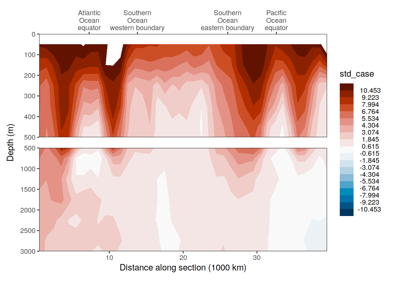
dcant_global_section_all_uncertainty  %>%
  filter(data_source == "obs",
         period == "1994 - 2004") %>%
  p_section_global(
    var = "sd",
    plot_slabs = "n",
    title_text = NULL,
    subtitle_text = NULL,
    col = "div"
  )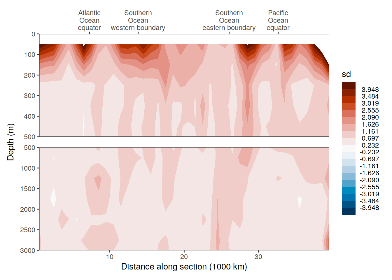
| Version | Author | Date |
|---|---|---|
| 8ded995 | jens-daniel-mueller | 2023-01-05 |
| 0f2c9d5 | jens-daniel-mueller | 2022-12-08 |
| 3a7bab0 | jens-daniel-mueller | 2022-11-28 |
| 322b1c1 | jens-daniel-mueller | 2022-11-25 |
| 491f8b1 | jens-daniel-mueller | 2022-11-25 |
| 4da4d66 | jens-daniel-mueller | 2022-11-25 |
| 534ee74 | jens-daniel-mueller | 2022-11-25 |
| e924c80 | jens-daniel-mueller | 2022-11-17 |
| 1dad51a | jens-daniel-mueller | 2022-11-15 |
| 6edad9b | jens-daniel-mueller | 2022-11-11 |
ggplot() +
  geom_point(
    data = dcant_global_section_all_uncertainty %>%
      filter(signif_single == 0),
    aes(dist, depth),
    shape = 4
  ) +
  facet_grid(data_source~period) +
  scale_y_reverse()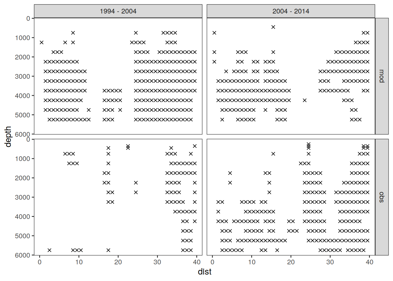
ggplot() +
  geom_point(
    data = dcant_global_section_all_uncertainty %>%
      filter(signif_double == 0),
    aes(dist, depth),
    shape = 4
  ) +
  facet_grid(data_source~period) +
  scale_y_reverse()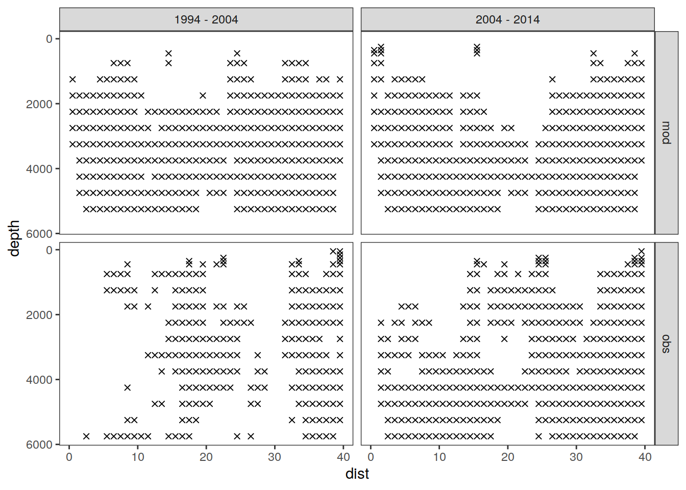
delta_dcant_global_section_all_uncertainty <-
  delta_dcant_global_section_all_uncertainty %>%
  mutate(band = "dummy")

delta_dcant_global_section_all_uncertainty  %>%
  filter(data_source == "obs") %>%
  p_section_global(
    var = "delta_dcant",
    plot_slabs = "n",
    title_text = NULL,
    subtitle_text = NULL,
    col = "div"
  )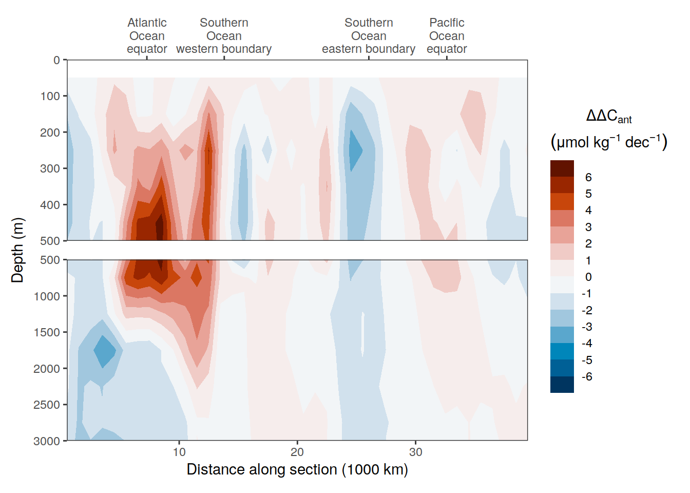
| Version | Author | Date |
|---|---|---|
| 8ded995 | jens-daniel-mueller | 2023-01-05 |
| 0f2c9d5 | jens-daniel-mueller | 2022-12-08 |
| 3a7bab0 | jens-daniel-mueller | 2022-11-28 |
| 322b1c1 | jens-daniel-mueller | 2022-11-25 |
| 491f8b1 | jens-daniel-mueller | 2022-11-25 |
| 4da4d66 | jens-daniel-mueller | 2022-11-25 |
| 534ee74 | jens-daniel-mueller | 2022-11-25 |
| 5520de8 | jens-daniel-mueller | 2022-11-15 |
| 1dad51a | jens-daniel-mueller | 2022-11-15 |
| 6edad9b | jens-daniel-mueller | 2022-11-11 |
delta_dcant_global_section_all_uncertainty  %>%
  filter(data_source == "obs") %>%
  select(-delta_dcant) %>%
  rename(delta_dcant = RSS) %>%
  p_section_global(
    var = "delta_dcant",
    plot_slabs = "n",
    title_text = NULL,
    subtitle_text = NULL,
    col = "div"
  )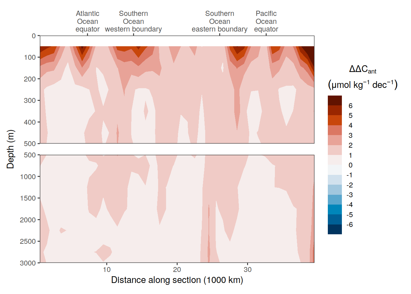
| Version | Author | Date |
|---|---|---|
| 8ded995 | jens-daniel-mueller | 2023-01-05 |
| 0f2c9d5 | jens-daniel-mueller | 2022-12-08 |
| 3a7bab0 | jens-daniel-mueller | 2022-11-28 |
| 322b1c1 | jens-daniel-mueller | 2022-11-25 |
| 491f8b1 | jens-daniel-mueller | 2022-11-25 |
| 4da4d66 | jens-daniel-mueller | 2022-11-25 |
| 534ee74 | jens-daniel-mueller | 2022-11-25 |
| 1dad51a | jens-daniel-mueller | 2022-11-15 |
| 6edad9b | jens-daniel-mueller | 2022-11-11 |
ggplot() +
  geom_point(
    data = delta_dcant_global_section_all_uncertainty %>%
      filter(signif_single == 0),
    aes(dist, depth),
    shape = 4
  ) +
  scale_y_reverse() +
  facet_grid(data_source~.)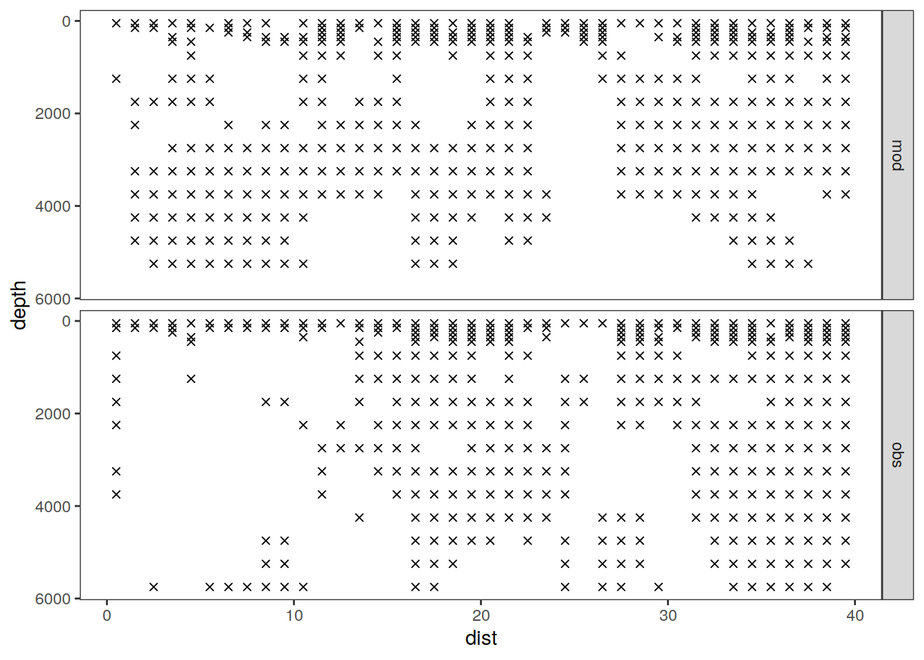
ggplot() +
  geom_point(
    data = delta_dcant_global_section_all_uncertainty %>%
      filter(signif_double == 0),
    aes(dist, depth),
    shape = 4
  ) +
  scale_y_reverse() +
  facet_grid(data_source~.)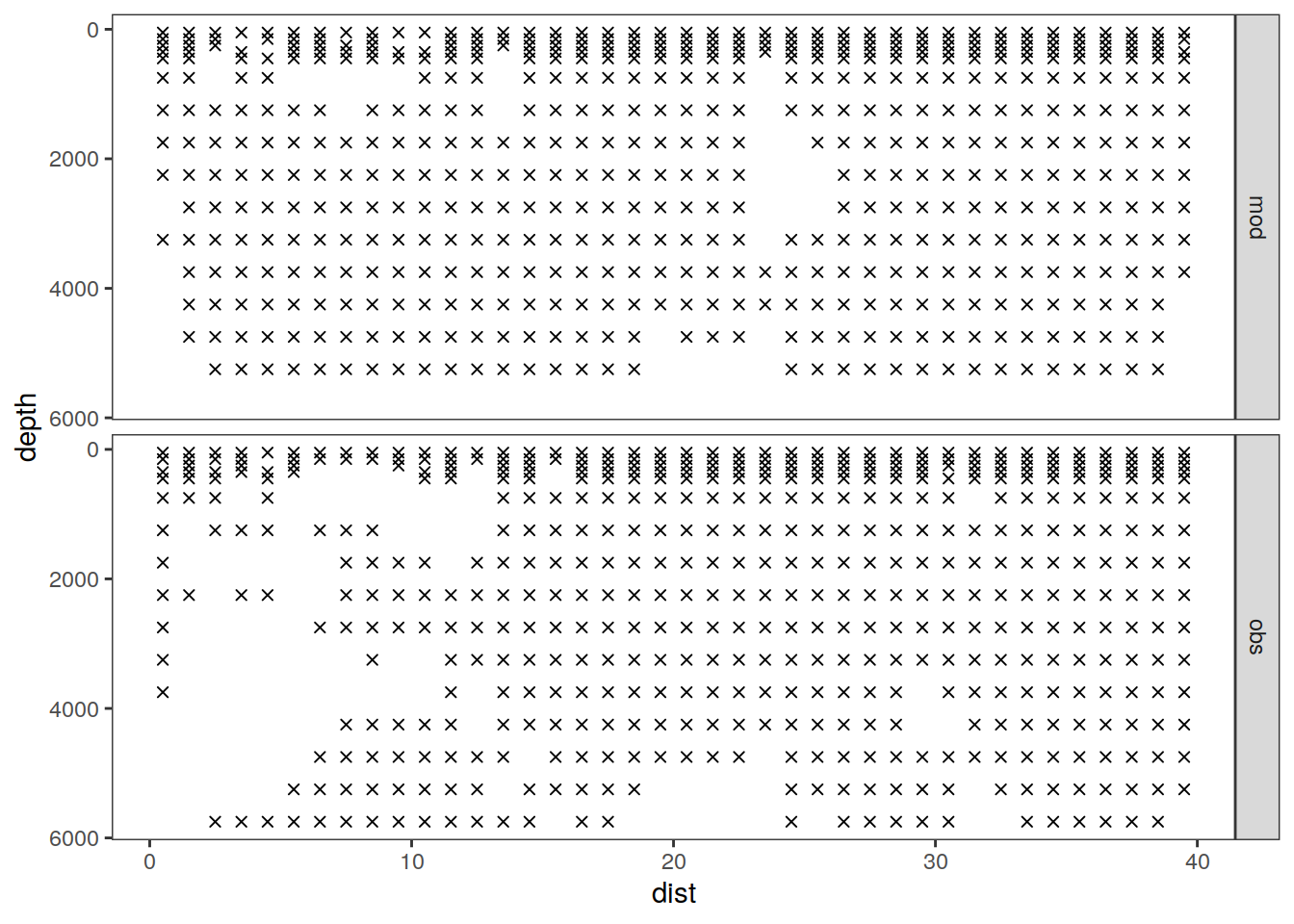
10.2 Observations
dcant_global_section_all_inv <- dcant_global_section_all_ensemble %>%
  select(data_source, period, depth, lat = dist, basin_AIP = band,
         dcant, dcant_pos, Version_ID_group, MLR_basins) %>%
  mutate(lon = "dummy") %>%
  group_by(data_source, period, Version_ID_group, MLR_basins) %>%
  nest() %>%
  mutate(inv = map(.x = data, ~m_dcant_inv(.x))) %>%
  select(-data) %>%
  unnest(inv) %>%
  rename(dist = lat, band = basin_AIP) %>%
  select(-lon)

# dcant_global_section_all_inv %>%
#   filter(period %in% two_decades) %>%
#   ggplot(aes(dist, dcant, col = as.factor(inv_depth))) +
#   geom_path(size = 2) +
#   scale_color_viridis_d(direction = -1) +
#   coord_cartesian(ylim = c(0,20)) +
#   facet_grid(data_source ~ period)

dcant_global_section_all_inv %>%
  filter(period %in% two_decades,
         inv_depth == 3000) %>%
  ggplot(aes(dist, dcant, col = MLR_basins, group = interaction(Version_ID_group, MLR_basins))) +
  geom_path() +
  scale_color_brewer(palette = "Dark2") +
  coord_cartesian(ylim = c(0,20)) +
  facet_grid(data_source ~ period)

dcant_global_section_all_surface <- dcant_global_section_all_ensemble %>%
  select(data_source, period, depth, dist, band, dcant, Version_ID_group, MLR_basins) %>%
  group_by(data_source) %>%
  mutate(surface_depth = min(depth, na.rm = TRUE)) %>%
  ungroup() %>%
  filter(depth == surface_depth) %>%
  select(-surface_depth) %>%
  rename(dcant_surface = dcant)

dcant_global_section_all_surface %>%
  filter(period %in% two_decades) %>%
  arrange(dist) %>%
  ggplot(aes(dist, dcant_surface, col = Version_ID_group, group = interaction(Version_ID_group, MLR_basins))) +
  geom_path() +
  scale_color_brewer(palette = "Dark2") +
  # coord_cartesian(ylim = c(0,20)) +
  facet_grid(data_source ~ period)

dcant_global_section_all_penetration <-
  full_join(dcant_global_section_all_surface,
            dcant_global_section_all_inv)

dcant_global_section_all_penetration <-
  dcant_global_section_all_penetration %>%
  mutate(dcant_surface = dcant_surface * 1e3 * 1.025 / 1e6,
         depth =  dcant / dcant_surface)

dcant_global_section_all_penetration <-
  dcant_global_section_all_penetration %>%
  filter(period %in% two_decades,
         inv_depth == 3000) %>%
  arrange(dist)

dcant_global_section_all_penetration %>%
  ggplot(aes(dist, depth, col = Version_ID_group, group = interaction(Version_ID_group, MLR_basins))) +
  geom_path() +
  scale_y_reverse(limits = c(3000,0)) +
  scale_color_brewer(palette = "Dark2") +
  # coord_cartesian(ylim = c(0,20)) +
  facet_grid(data_source ~ period)

dcant_global_section_all_penetration_uncertainty <-
  additive_uncertainty(dcant_global_section_all_penetration %>%
          select(-c(dcant, dcant_pos, dcant_surface, inv_depth)) %>%
            group_by(data_source, period, dist, Version_ID_group, MLR_basins) %>%
            summarise(dcant = mean(depth, na.rm = TRUE)) %>%
            ungroup())

delta_dcant_global_section_all_penetration_uncertainty <- dcant_global_section_all_penetration_uncertainty[[3]]
dcant_global_section_all_penetration_uncertainty <- dcant_global_section_all_penetration_uncertainty[[1]]


dcant_global_section_all_penetration_uncertainty %>%
  ggplot(aes(dist,
             std_case,
             ymin = std_case - sd,
             ymax = std_case + sd,
             fill = period)) +
  geom_ribbon(alpha = 0.3) +
  geom_path(aes(col = period)) +
  scale_y_reverse() +
  scale_color_brewer(palette = "Dark2") +
  scale_fill_brewer(palette = "Dark2") +
  coord_cartesian(ylim = c(3000,0)) +
  facet_grid(data_source ~ .)

delta_dcant_global_section_all_penetration_uncertainty %>%
  ggplot(aes(dist,
             delta_dcant,
             ymin = delta_dcant - RSS,
             ymax = delta_dcant + RSS)) +
  geom_hline(yintercept = 0) +
  geom_ribbon(alpha = 0.3) +
  geom_path() +
  scale_y_reverse() +
  scale_color_brewer(palette = "Dark2") +
  scale_fill_brewer(palette = "Dark2") +
  coord_cartesian(ylim = c(1000,-1000)) +
  facet_grid(data_source ~ period)
p_dcant_global_section_dec1 <- dcant_global_section_all %>%
filter(data_source == "obs",
period %in% "1994 - 2004") %>%
p_section_global(
var = "dcant",
title_text = "A 1994 – 2004",
df_uncertainty = dcant_global_section_all_uncertainty %>%
filter(period %in% "1994 - 2004",
data_source == "obs"),
# df_penetration = dcant_global_section_all_penetration %>%
# filter(data_source == "obs",
# period %in% "1994 - 2004"),
col_uncertainty = "grey",
subtitle_text = NULL,
plot_slabs = "n",
contour_level = 5
) &
theme(axis.title.x = element_blank(),
axis.text.x.bottom = element_blank())
p_dcant_global_section_dec1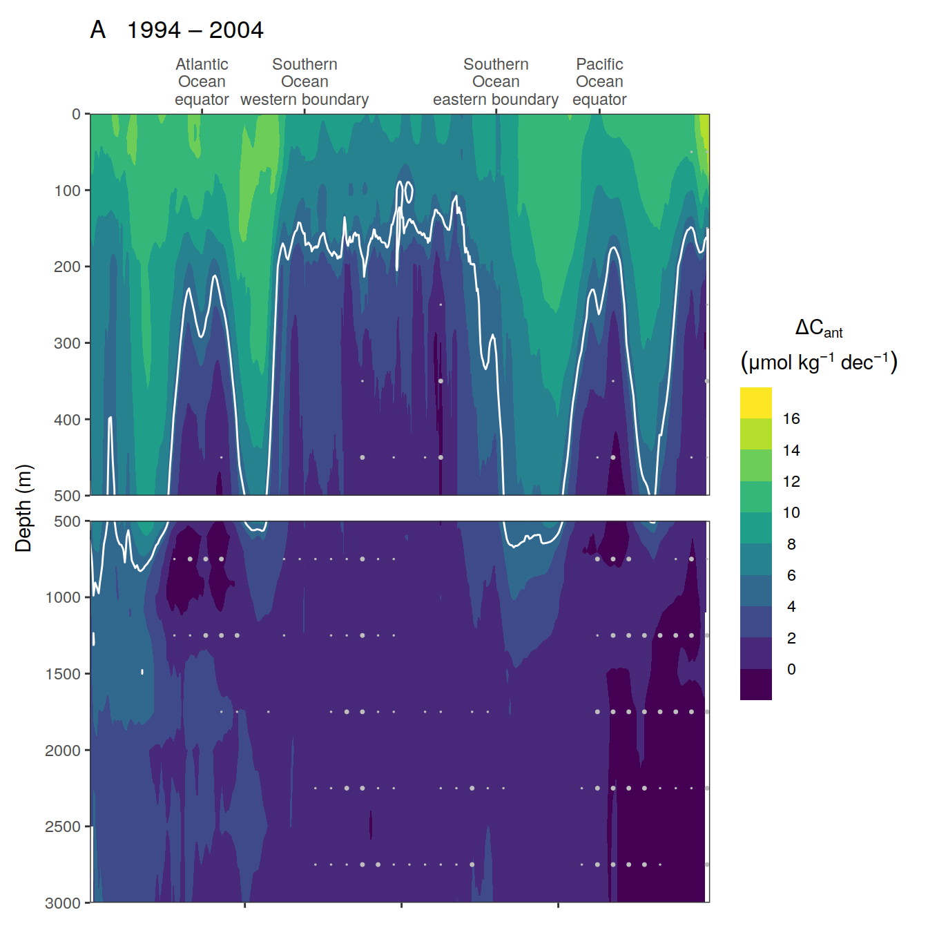
| Version | Author | Date |
|---|---|---|
| 8ded995 | jens-daniel-mueller | 2023-01-05 |
| 0f2c9d5 | jens-daniel-mueller | 2022-12-08 |
| 3a7bab0 | jens-daniel-mueller | 2022-11-28 |
| 322b1c1 | jens-daniel-mueller | 2022-11-25 |
| 491f8b1 | jens-daniel-mueller | 2022-11-25 |
| 4da4d66 | jens-daniel-mueller | 2022-11-25 |
| 534ee74 | jens-daniel-mueller | 2022-11-25 |
| 5520de8 | jens-daniel-mueller | 2022-11-15 |
| 1dad51a | jens-daniel-mueller | 2022-11-15 |
| 6edad9b | jens-daniel-mueller | 2022-11-11 |
| 16beb51 | jens-daniel-mueller | 2022-11-08 |
| b92657d | jens-daniel-mueller | 2022-11-08 |
| 7275091 | jens-daniel-mueller | 2022-11-05 |
p_dcant_global_section_dec2 <-
  dcant_global_section_all %>%
  filter(data_source == "obs",
         period %in% "2004 - 2014") %>%
  p_section_global(
    var = "dcant",
    title_text = "B   2004 – 2014",
    subtitle_text = NULL,
    plot_slabs = "n",
    contour_level = 5,
    df_uncertainty = dcant_global_section_all_uncertainty %>%
      filter(period %in% "2004 - 2014",
             data_source == "obs"),
    col_uncertainty = "grey",
    # df_penetration = dcant_global_section_all_penetration %>%
    #   filter(data_source == "obs",
    #          period %in% "2004 - 2014")
  )&
  theme(legend.position = "none")

p_dcant_global_section_offset <-
  dcant_global_section_all %>%
  filter(data_source == "obs",
         period %in% two_decades) %>%
  arrange(depth, dist) %>%
  select(depth, dist, dcant, period, gamma_mean) %>%
  drop_na() %>%
  pivot_wider(names_from = period,
              values_from = dcant) %>%
  mutate(delta_dcant = `2004 - 2014` - `1994 - 2004`) %>%
  p_section_global(
    var = "delta_dcant",
    df_uncertainty = delta_dcant_global_section_all_uncertainty %>%
      filter(data_source == "obs"),
    plot_slabs = "y",
    col = "div",
    title_text = "C   Decadal difference",
    subtitle_text = NULL
  )

wrap_plots(
  p_dcant_global_section_dec1,
  p_dcant_global_section_dec2 &
    theme(axis.title.x = element_blank(),
          axis.text.x = element_blank()
          ),
  p_dcant_global_section_offset &
    theme(
      axis.text.x.top = element_blank()
      ),
  ncol = 1
)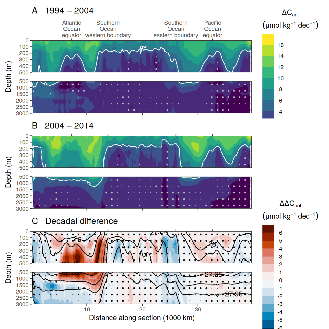
| Version | Author | Date |
|---|---|---|
| 8ded995 | jens-daniel-mueller | 2023-01-05 |
ggsave(path = here::here("output/publication"),
       filename = "Fig_dcant_global_section.png",
       height = 10,
       width = 8,
       dpi = 600)

ggsave(path = here::here("output/presentation"),
       filename = "Fig_dcant_global_section.png",
       height = 9,
       width = 10,
       dpi = 600)

rm(p_dcant_global_section_dec1, p_dcant_global_section_dec2,
   p_dcant_global_section_offset)
10.3 Synthetic data
p_dcant_global_section_dec1 <-
  dcant_global_section_all %>%
  filter(data_source == "mod",
         period %in% "1994 - 2004") %>%
  p_section_global(var = "dcant",
                   title_text = "1994 - 2004",
                   df_uncertainty = dcant_global_section_all_uncertainty %>%
                     filter(period %in% "1994 - 2004",
                            data_source == "mod"),
                   col_uncertainty = "grey",
                   subtitle_text = NULL,
                   plot_slabs = "n",
                   contour_level = 5) +
  theme(
    axis.title.x = element_blank(),
    axis.text.x.bottom = element_blank()
  )


p_dcant_global_section_dec2 <-
  dcant_global_section_all %>%
  filter(data_source == "mod",
         period %in% "2004 - 2014") %>%
  p_section_global(
    var = "dcant",
    title_text = NULL,
    subtitle_text = NULL,
    plot_slabs = "n",
    contour_level = 5,
    df_uncertainty = dcant_global_section_all_uncertainty %>%
      filter(period %in% "2004 - 2014",
                            data_source == "mod"),
    col_uncertainty = "grey"
  ) &
  theme(
    legend.position = "none"
  )

p_dcant_global_section_offset <-
  dcant_global_section_all %>%
  filter(data_source == "mod",
         period %in% two_decades) %>%
  arrange(depth, dist) %>%
  select(depth, dist, dcant, period, gamma_mean) %>%
  drop_na() %>%
  group_by(depth, dist) %>%
  mutate(gamma_mean = mean(gamma_mean)) %>%
  ungroup() %>%
  pivot_wider(names_from = period,
              values_from = dcant) %>%
  mutate(delta_dcant = `2004 - 2014` - `1994 - 2004`) %>%
  p_section_global(
    var = "delta_dcant",
    df_uncertainty = delta_dcant_global_section_all_uncertainty %>%
      filter(data_source == "mod"),
    col = "div",
    plot_slabs = "y",
    title_text = NULL,
    subtitle_text = NULL
  )


wrap_plots(
  p_dcant_global_section_dec1,
  p_dcant_global_section_dec2 &
    theme(axis.title.x = element_blank(),
          axis.text.x = element_blank()),
  p_dcant_global_section_offset &
    theme(axis.title.x.top = element_blank(),
          axis.text.x.top = element_blank()),
  ncol = 1
)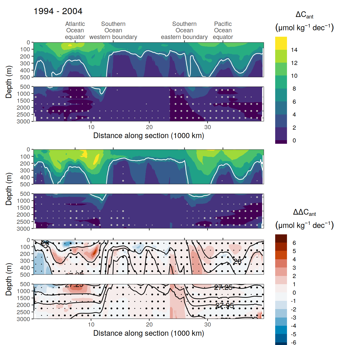
| Version | Author | Date |
|---|---|---|
| 8ded995 | jens-daniel-mueller | 2023-01-05 |
| 0f2c9d5 | jens-daniel-mueller | 2022-12-08 |
| 3a7bab0 | jens-daniel-mueller | 2022-11-28 |
| 322b1c1 | jens-daniel-mueller | 2022-11-25 |
| 491f8b1 | jens-daniel-mueller | 2022-11-25 |
| 4da4d66 | jens-daniel-mueller | 2022-11-25 |
| 534ee74 | jens-daniel-mueller | 2022-11-25 |
| 5520de8 | jens-daniel-mueller | 2022-11-15 |
| 1dad51a | jens-daniel-mueller | 2022-11-15 |
| 6edad9b | jens-daniel-mueller | 2022-11-11 |
| 16beb51 | jens-daniel-mueller | 2022-11-08 |
| b92657d | jens-daniel-mueller | 2022-11-08 |
| 7275091 | jens-daniel-mueller | 2022-11-05 |
ggsave(path = here::here("output/publication"),
       filename = "FigS_dcant_global_section_synthetic_data.png",
       height = 10,
       width = 8,
       dpi = 600)

rm(p_dcant_global_section_dec1, p_dcant_global_section_dec2,
   p_dcant_global_section_offset)
11 Zonal sections
11.1 Additive uncertainty
delta_dcant_zonal_all <-
  dcant_zonal_all %>%
  filter(data_source %in% c("obs", "mod"),
         period %in% two_decades) %>%
  select(data_source, lat, depth, period, basin_AIP, dcant) %>%
  drop_na() %>%
  pivot_wider(names_from = period,
              values_from = dcant) %>%
  mutate(dcant_offset = `2004 - 2014` - `1994 - 2004`,
         period = "(2004 - 2014) - (1994 - 2004)")

dcant_zonal_all_uncertainty <-
  dcant_zonal_all_ensemble %>%
  filter(data_source %in% c("obs", "mod"),
         period %in% two_decades) %>%
  select(lat,
         depth,
         period,
         basin_AIP,
         data_source,
         MLR_basins,
         Version_ID_group,
         dcant) %>%
  mutate(lat_grid = as.numeric(as.character(cut(
    lat, seq(-90, 90, 10), seq(-85, 85, 10)
  ))),
  # depth_grid = depth
  depth_grid = as.numeric(as.character(cut(
    depth,
    c(seq(0, 500, 100), seq(1000, 10000, 500)),
    c(seq(50, 450, 100), seq(750, 10000, 500)),
    right = FALSE
  )))
  ) %>%
  group_by(lat_grid,
           depth_grid,
           data_source,
           period,
           basin_AIP,
           MLR_basins,
           Version_ID_group) %>%
  summarise(dcant = mean(dcant)) %>%
  ungroup() %>%
  rename(lat = lat_grid,
         depth = depth_grid)

dcant_zonal_all_uncertainty <-
  additive_uncertainty(dcant_zonal_all_uncertainty)


delta_dcant_zonal_all_uncertainty <- dcant_zonal_all_uncertainty[[3]]
dcant_zonal_all_uncertainty <- dcant_zonal_all_uncertainty[[1]]

dcant_zonal_all_uncertainty  %>%
  filter(data_source == "obs") %>%
  p_section_zonal_continous_depth(
    var = "std_case",
    plot_slabs = "n",
    title_text = NULL,
    subtitle_text = NULL,
    col = "div"
  ) +
  facet_grid(period~basin_AIP)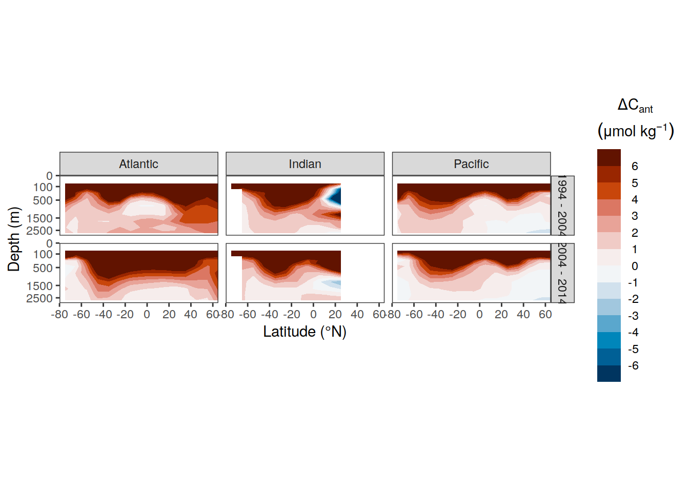
| Version | Author | Date |
|---|---|---|
| 3a7bab0 | jens-daniel-mueller | 2022-11-28 |
dcant_zonal_all_uncertainty  %>%
  filter(data_source == "obs") %>%
  p_section_zonal_continous_depth(
    var = "sd",
    plot_slabs = "n",
    title_text = NULL,
    subtitle_text = NULL,
    col = "div"
  ) +
  facet_grid(period ~ basin_AIP)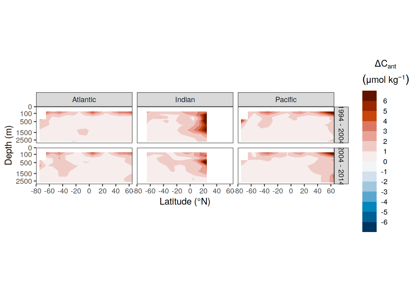
| Version | Author | Date |
|---|---|---|
| 3a7bab0 | jens-daniel-mueller | 2022-11-28 |
ggplot() +
  geom_point(
    data = dcant_zonal_all_uncertainty %>%
      filter(signif_single == 0,
             data_source == "obs"),
    aes(lat, depth),
    shape = 4
  ) +
  facet_grid(period ~ basin_AIP) +
  scale_y_reverse()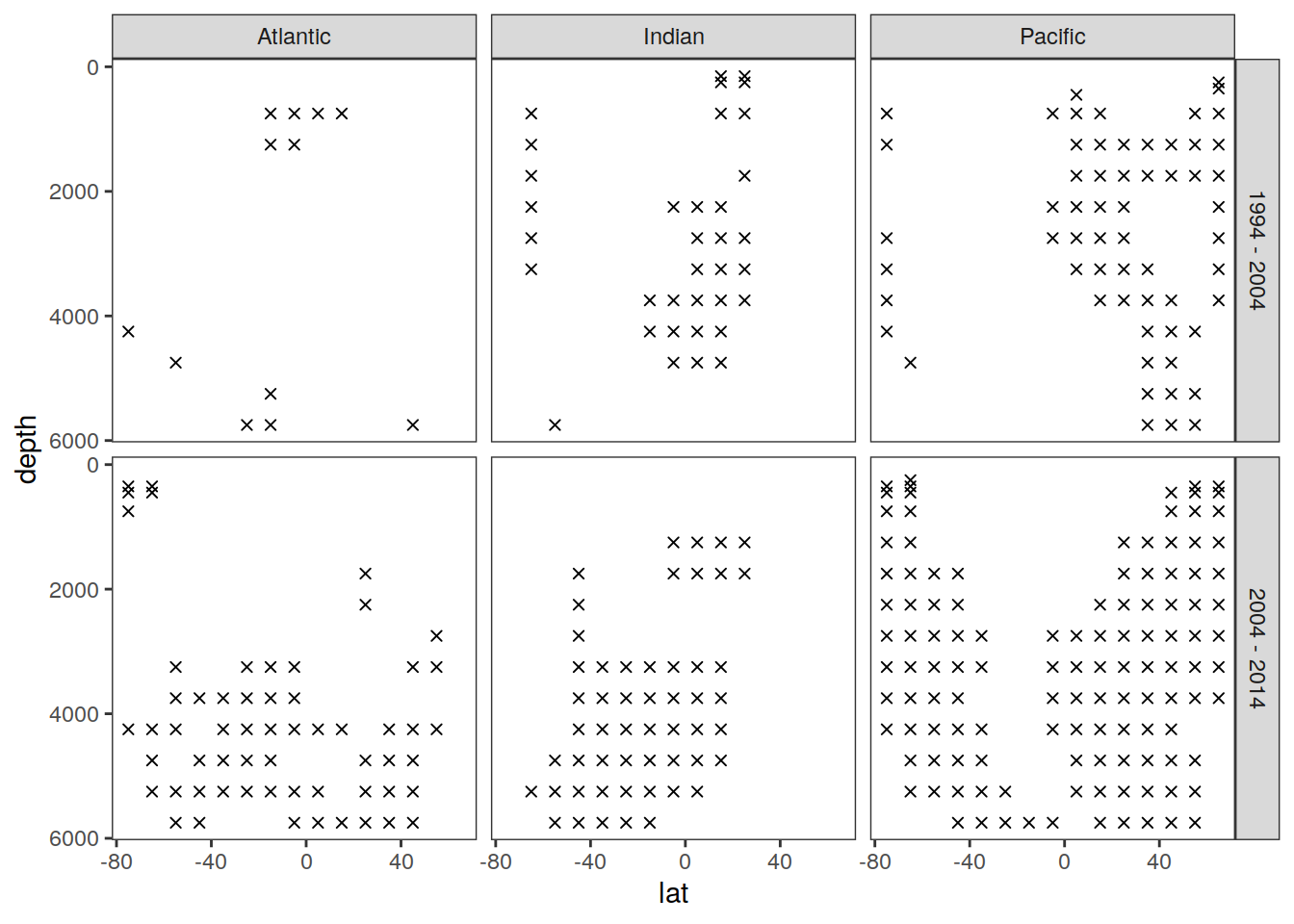
| Version | Author | Date |
|---|---|---|
| 3a7bab0 | jens-daniel-mueller | 2022-11-28 |
ggplot() +
  geom_point(
    data = dcant_zonal_all_uncertainty %>%
      filter(signif_double == 0,
             data_source == "obs"),
    aes(lat, depth),
    shape = 4
  ) +
  facet_grid(period ~ basin_AIP) +
  scale_y_reverse()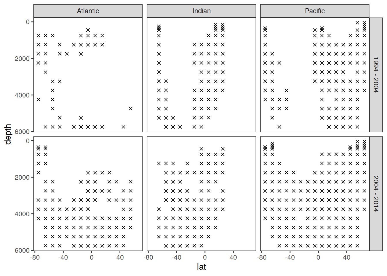
| Version | Author | Date |
|---|---|---|
| 3a7bab0 | jens-daniel-mueller | 2022-11-28 |
delta_dcant_zonal_all_uncertainty  %>%
  filter(data_source == "obs") %>%
  p_section_zonal_continous_depth(
    var = "delta_dcant",
    plot_slabs = "n",
    title_text = NULL,
    subtitle_text = NULL,
    col = "div"
  ) +
  facet_grid(. ~ basin_AIP)
| Version | Author | Date |
|---|---|---|
| 3a7bab0 | jens-daniel-mueller | 2022-11-28 |
delta_dcant_zonal_all_uncertainty  %>%
  filter(data_source == "obs") %>%
  select(-delta_dcant) %>%
  rename(delta_dcant = RSS) %>%
  p_section_zonal_continous_depth(
    var = "delta_dcant",
    plot_slabs = "n",
    title_text = NULL,
    subtitle_text = NULL,
    col = "div"
  ) +
  facet_grid(. ~ basin_AIP)
| Version | Author | Date |
|---|---|---|
| 3a7bab0 | jens-daniel-mueller | 2022-11-28 |
ggplot() +
  geom_point(
    data = delta_dcant_zonal_all_uncertainty %>%
      filter(signif_single == 0),
    aes(lat, depth),
    shape = 4
  ) +
  scale_y_reverse() +
  facet_grid(data_source~basin_AIP)
| Version | Author | Date |
|---|---|---|
| 3a7bab0 | jens-daniel-mueller | 2022-11-28 |
ggplot() +
  geom_point(
    data = delta_dcant_zonal_all_uncertainty %>%
      filter(signif_double == 0),
    aes(lat, depth),
    shape = 4
  ) +
  scale_y_reverse() +
  facet_grid(data_source~basin_AIP)
| Version | Author | Date |
|---|---|---|
| 3a7bab0 | jens-daniel-mueller | 2022-11-28 |
11.2 dcant - absolut
p_dcant_zonal_absolute <-
  dcant_zonal_all %>%
  filter(
    data_source == "obs",
    period %in% two_decades,
    depth <= params_global$inventory_depth_standard
  ) %>%
  p_section_zonal_continous_depth(var = "dcant",
                                  plot_slabs = "n",
                                  title_text = NULL) +
  geom_contour(aes(lat, depth, z = dcant),
               breaks = 5,
               col = "white") +
  # geom_point(
  #   data = dcant_zonal_all_uncertainty %>% filter(signif_single == 0),
  #   aes(lat, depth),
  #   shape = 20,
  #   size = 1,
  #   col = "grey"
  # ) +
  # geom_point(
  #   data = dcant_zonal_all_uncertainty %>% filter(signif_double == 0),
  #   aes(lat, depth),
  #   shape = 20,
  #   size = 0.1,
  #   col = "grey"
  # )+
  # geom_text_contour(
  #   aes(lat, depth, z = dcant),
  #   breaks = 5,
  #   stroke = 0.2,
  #   stroke.colour = "white",
  #   rotate = FALSE,
  #   label.placer = label_placer_n(n = 1)
  # ) +
  facet_grid(period ~ basin_AIP) +
  theme(
    axis.text.x = element_blank(),
    axis.title.x = element_blank(),
    legend.position = "top"
  ) +
  guides(fill = guide_colorsteps(
    barheight = unit(0.5, "cm"),
    barwidth = unit(7, "cm"),
    show.limits = FALSE
  ))

p_dcant_zonal_absolute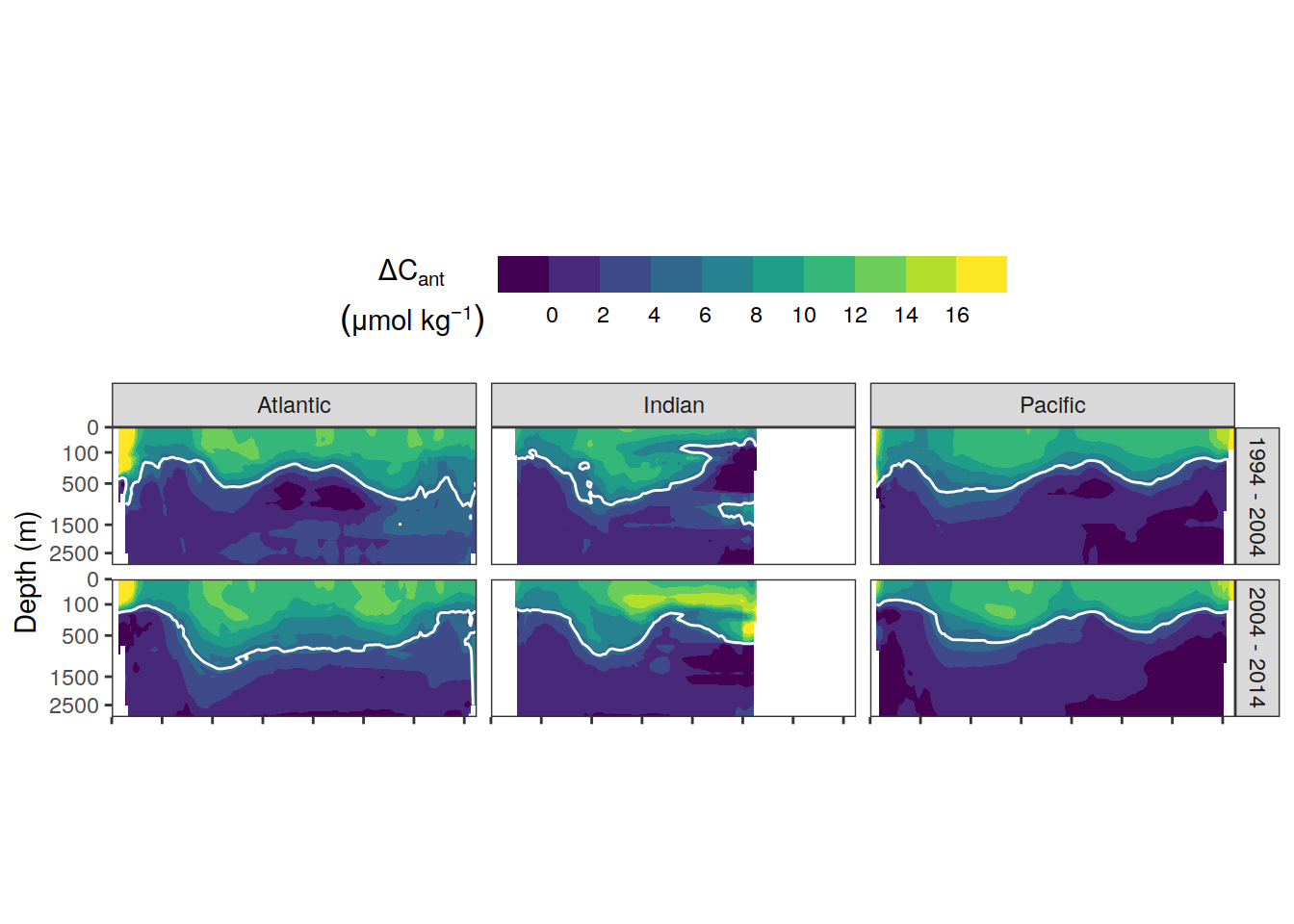
| Version | Author | Date |
|---|---|---|
| 3a7bab0 | jens-daniel-mueller | 2022-11-28 |
| 2345935 | jens-daniel-mueller | 2022-10-29 |
| 051b911 | jens-daniel-mueller | 2022-09-07 |
| 75bd58c | jens-daniel-mueller | 2022-09-07 |
| 1c6de0d | jens-daniel-mueller | 2022-09-07 |
| 78dbb27 | jens-daniel-mueller | 2022-08-11 |
| 302d289 | jens-daniel-mueller | 2022-08-11 |
| f68fcfa | jens-daniel-mueller | 2022-07-26 |
| f2615fb | jens-daniel-mueller | 2022-07-26 |
| e2adac6 | jens-daniel-mueller | 2022-07-22 |
| fea41c1 | jens-daniel-mueller | 2022-07-20 |
| d2ae54c | jens-daniel-mueller | 2022-07-18 |
| ea46812 | jens-daniel-mueller | 2022-07-13 |
| 16dc3af | jens-daniel-mueller | 2022-06-27 |
| 87e9eb8 | jens-daniel-mueller | 2022-06-27 |
| b52b159 | jens-daniel-mueller | 2022-06-27 |
| 09b0780 | jens-daniel-mueller | 2022-05-24 |
| 1d73ec9 | jens-daniel-mueller | 2022-05-16 |
| 2ca0109 | jens-daniel-mueller | 2022-05-02 |
| b018a9a | jens-daniel-mueller | 2022-04-29 |
| e09320d | jens-daniel-mueller | 2022-04-12 |
| acad2e2 | jens-daniel-mueller | 2022-04-09 |
| 3d81135 | jens-daniel-mueller | 2022-04-07 |
| a74e341 | jens-daniel-mueller | 2022-04-04 |
| bd9e11d | jens-daniel-mueller | 2022-03-22 |
| 2501978 | jens-daniel-mueller | 2022-03-21 |
| 094bfa0 | jens-daniel-mueller | 2022-02-18 |
| d2191ad | jens-daniel-mueller | 2022-02-04 |
| 5f2aed0 | jens-daniel-mueller | 2022-01-27 |
| 9753eb8 | jens-daniel-mueller | 2022-01-26 |
| b1d7720 | jens-daniel-mueller | 2022-01-21 |
| e572075 | jens-daniel-mueller | 2022-01-21 |
11.3 dcant - absolute delta
dcant_zonal_all %>%
  filter(data_source %in% c("mod", "obs"),
         period != "1994 - 2014") %>%
  select(data_source, lat, depth, basin_AIP, period, dcant) %>%
  pivot_wider(names_from = period,
              values_from = dcant) %>%
  mutate(delta_dcant = `2004 - 2014` - `1994 - 2004`) %>%
  group_by(data_source) %>%
  group_split() %>%
  # head(1) %>%
  map(
    ~ p_section_zonal_continous_depth(
      df = .x,
      var = "delta_dcant",
      plot_slabs = "n",
      subtitle_text = unique(.x$data_source),
      col = "bias"
    ) +
      facet_grid(basin_AIP ~ .)
  )
[[1]]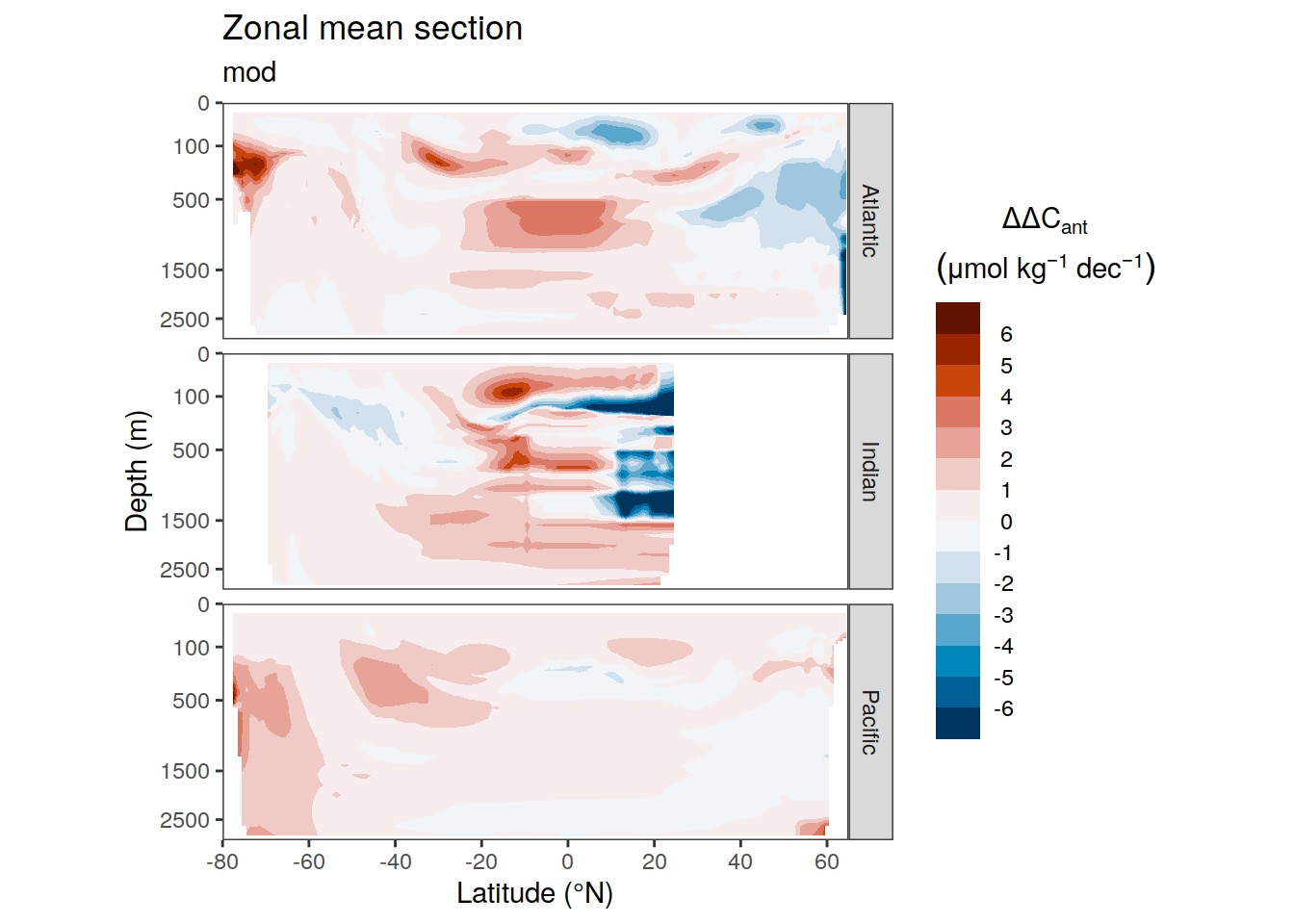
[[2]]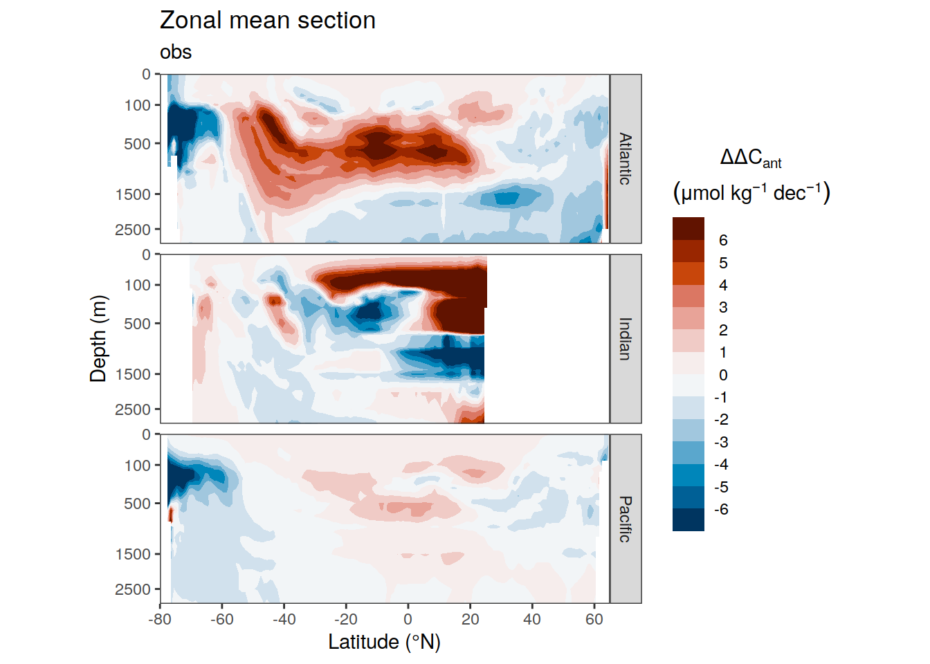
p_dcant_zonal_delta <-
  dcant_zonal_all %>%
  filter(data_source %in% c("obs"),
         period != "1994 - 2014") %>%
  select(data_source, lat, depth, basin_AIP, period, gamma_mean, dcant) %>%
  pivot_wider(names_from = period,
              values_from = dcant) %>%
  mutate(delta_dcant = `2004 - 2014` - `1994 - 2004`) %>%
  p_section_zonal_continous_depth(
    var = "delta_dcant",
    plot_slabs = "y",
    drop_slabs = 1,
    subtitle_text = NULL,
    title_text = NULL,
    col = "bias"
  ) +
  # geom_point(
  #   data = delta_dcant_zonal_all_uncertainty %>% filter(signif_single == 0),
  #   aes(lat, depth),
  #   shape = 20,
  #   size = 1,
  #   col = "black"
  # ) +
  # geom_point(
  #   data = delta_dcant_zonal_all_uncertainty %>% filter(signif_double == 0),
  #   aes(lat, depth),
  #   shape = 20,
  #   size = 0.1,
  #   col = "black"
  # ) +
  facet_grid("Dec. diff." ~ basin_AIP) +
  theme(
    strip.text.x = element_blank(),
    strip.background.x = element_blank(),
    legend.position = "bottom"
  ) +
  guides(fill = guide_colorsteps(
    barheight = unit(0.5, "cm"),
    barwidth = unit(10, "cm"),
    show.limits = FALSE
  ))

p_dcant_zonal_absolute / p_dcant_zonal_delta +
  plot_layout(heights = c(2,1)) +
  plot_annotation(tag_levels = 'A')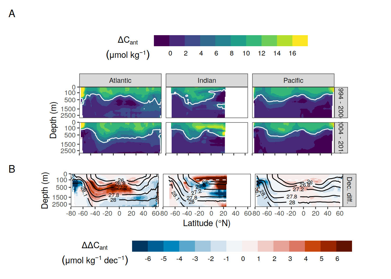
ggsave(path = here::here("output/publication"),
       filename = "FigS_dcant_zonal_mean_section.png",
       height = 6,
       width = 8,
       dpi = 600)

rm(p_dcant_zonal_absolute, p_dcant_zonal_delta)
11.4 Bias
p_dcant_zonal_absolute_mod <-
  dcant_zonal_all %>%
  filter(
    data_source != "obs",
    period %in% two_decades,
    depth <= params_global$inventory_depth_standard
  ) %>%
    mutate(data_source = case_when(
    data_source == "mod" ~ "Reconstruction",
    data_source == "mod_truth" ~ "Model truth"
  )) %>%
  p_section_zonal_continous_depth(var = "dcant",
                                  plot_slabs = "n",
                                  title_text = NULL) +
  geom_contour(aes(lat, depth, z = dcant),
               breaks = 5,
               col = "white") +
  facet_nested(data_source+period ~ basin_AIP) +
  theme(
    axis.text.x = element_blank(),
    axis.title.x = element_blank(),
    legend.position = "top"
  ) +
  guides(fill = guide_colorsteps(
    barheight = unit(0.5, "cm"),
    barwidth = unit(7, "cm"),
    show.limits = FALSE
  ))

p_dcant_zonal_absolute_mod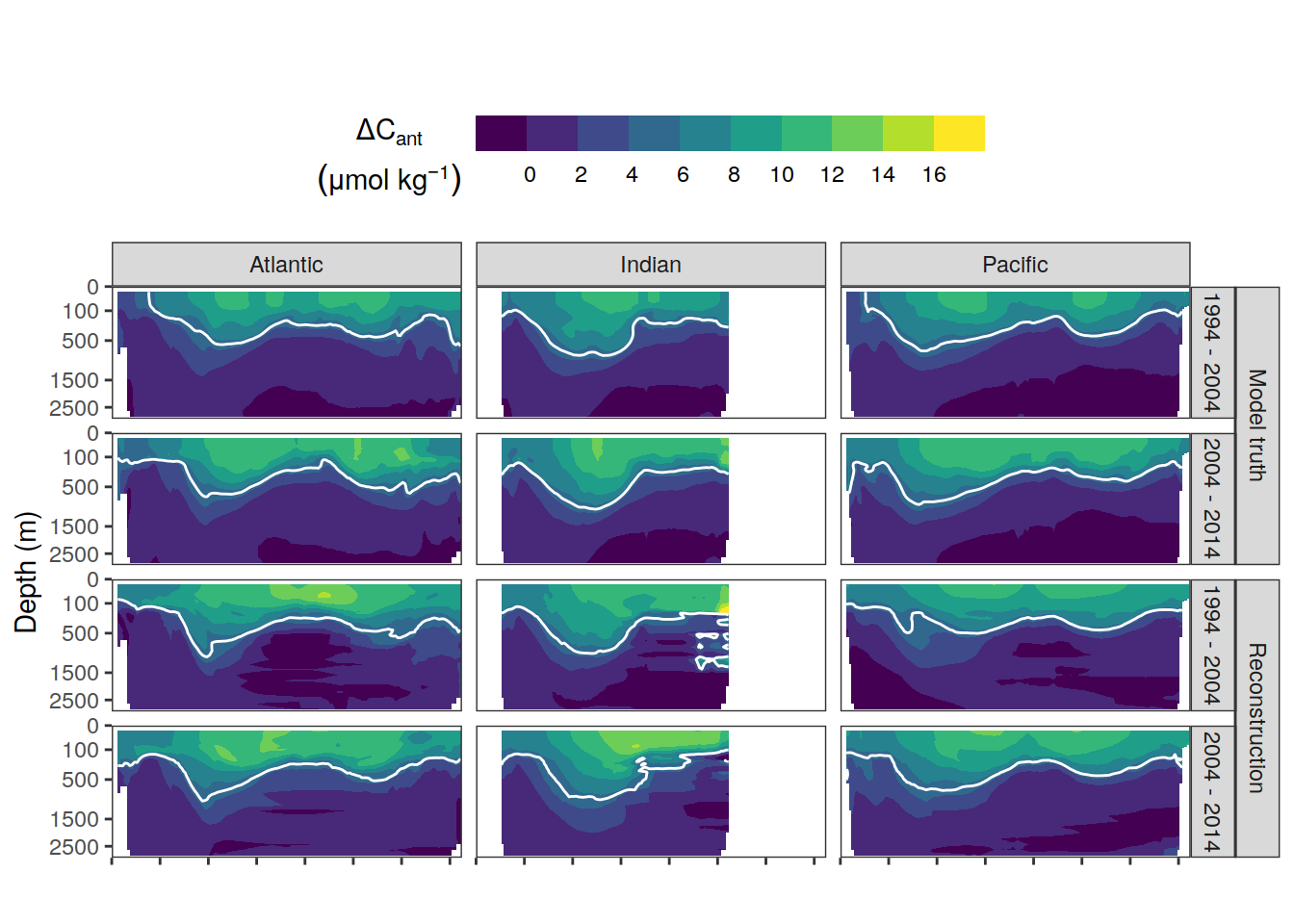
| Version | Author | Date |
|---|---|---|
| 3a7bab0 | jens-daniel-mueller | 2022-11-28 |
| 2345935 | jens-daniel-mueller | 2022-10-29 |
| 051b911 | jens-daniel-mueller | 2022-09-07 |
| 75bd58c | jens-daniel-mueller | 2022-09-07 |
| 1c6de0d | jens-daniel-mueller | 2022-09-07 |
| 78dbb27 | jens-daniel-mueller | 2022-08-11 |
| 302d289 | jens-daniel-mueller | 2022-08-11 |
| 5b77c4f | jens-daniel-mueller | 2022-08-10 |
p_dcant_zonal_bias <-
  dcant_zonal_all %>%
  filter(data_source != "obs",
         period %in% two_decades) %>%
  select(data_source, lat, depth, basin_AIP, period, dcant) %>%
  pivot_wider(names_from = data_source,
              values_from = dcant) %>%
  mutate(dcant_bias = mod - mod_truth) %>%
  p_section_zonal_continous_depth(
    var = "dcant_bias",
    plot_slabs = "n",
    drop_slabs = 1,
    subtitle_text = NULL,
    title_text = NULL,
    col = "bias"
  ) +
  facet_grid(period ~ basin_AIP) +
  theme(
    strip.text.x = element_blank(),
    strip.background.x = element_blank(),
    legend.position = "bottom"
  ) +
  guides(fill = guide_colorsteps(
    barheight = unit(0.5, "cm"),
    barwidth = unit(10, "cm"),
    show.limits = FALSE
  ))

p_dcant_zonal_absolute_mod / p_dcant_zonal_bias +
  plot_layout(heights = c(2,1)) +
  plot_annotation(tag_levels = 'A')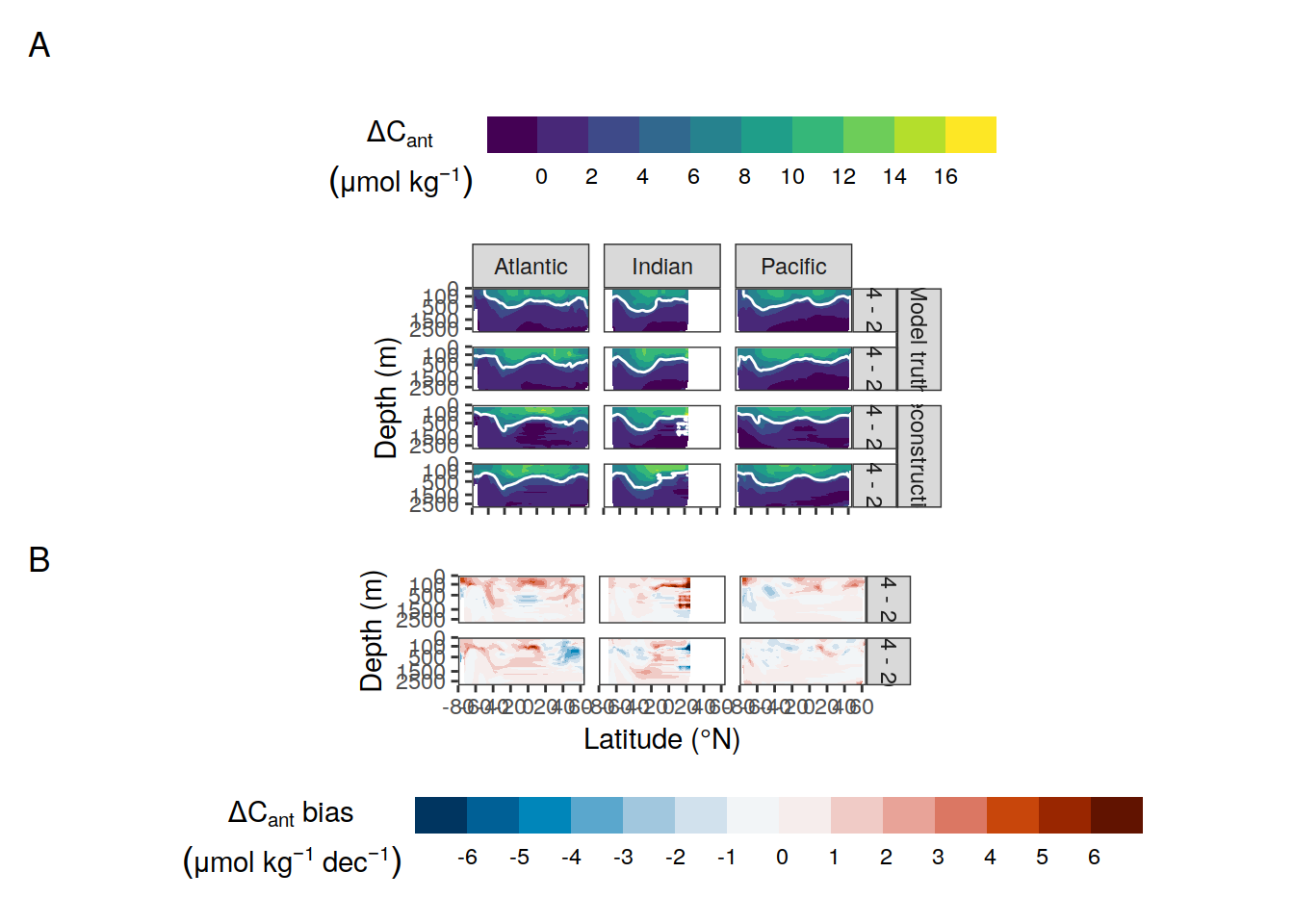
| Version | Author | Date |
|---|---|---|
| 3a7bab0 | jens-daniel-mueller | 2022-11-28 |
| 5520de8 | jens-daniel-mueller | 2022-11-15 |
| 2345935 | jens-daniel-mueller | 2022-10-29 |
| 46c163a | jens-daniel-mueller | 2022-10-10 |
| 051b911 | jens-daniel-mueller | 2022-09-07 |
| 75bd58c | jens-daniel-mueller | 2022-09-07 |
| 1c6de0d | jens-daniel-mueller | 2022-09-07 |
| 78dbb27 | jens-daniel-mueller | 2022-08-11 |
| 302d289 | jens-daniel-mueller | 2022-08-11 |
| 5b77c4f | jens-daniel-mueller | 2022-08-10 |
ggsave(
  path = here::here("output/publication"),
  filename = "FigS_dcant_zonal_mean_section_synthetic_data.png",
  height = 9,
  width = 8,
  dpi = 600
)

rm(p_dcant_zonal_absolute_mod,
   p_dcant_zonal_bias)
12 Penetration depth spatial
dcant_penetration_depth_all_lat_mean_all_ensemble %>%
  filter(dcant_lim == 5,
         period %in% two_decades,
         data_source != "obs") %>%
  mutate(
    data_source = case_when(
      data_source == "mod" ~ "Reconstruction\nensemble",
      data_source == "mod_truth" ~ "Model truth"
    ),
    data_source = fct_reorder(data_source, desc(data_source))
  ) %>%
  ggplot(aes(
    lat,
    depth_mean,
    group = interaction(MLR_basins, Version_ID_group, data_source)
  )) +
  geom_path(aes(col = data_source)) +
  geom_path(
    data = dcant_penetration_depth_all_lat_mean_all %>%
      filter(dcant_lim == 5,
             period %in% two_decades,
             data_source == "mod") %>%
      mutate(
        data_source = case_when(data_source == "mod" ~ "Standard case"),
        data_source = fct_reorder(data_source, desc(data_source))
      ),
    aes(lat,
        depth_mean,
        col = data_source)
  ) +
  scale_colour_manual(values = c("red", "grey", "black")) +
  labs(y = "Depth (m)",
       x = "Latitude (°N)") +
  theme(legend.title = element_blank()) +
  scale_y_reverse() +
  facet_grid(basin_AIP ~ period, scales = "free_x") +
  coord_cartesian(ylim = c(1500,0))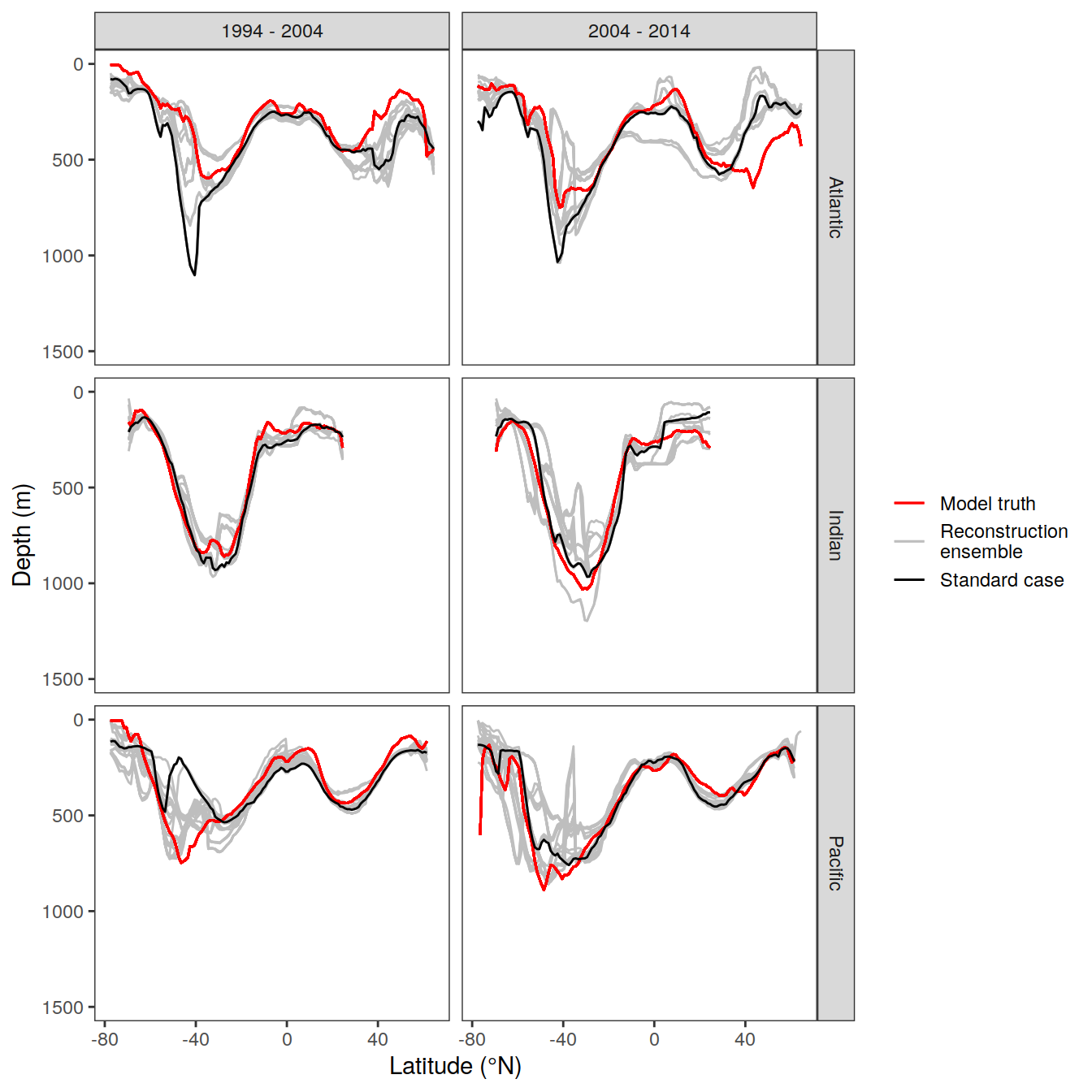
| Version | Author | Date |
|---|---|---|
| 0f2c9d5 | jens-daniel-mueller | 2022-12-08 |
| 3a7bab0 | jens-daniel-mueller | 2022-11-28 |
| 534ee74 | jens-daniel-mueller | 2022-11-25 |
| 1dad51a | jens-daniel-mueller | 2022-11-15 |
| 6edad9b | jens-daniel-mueller | 2022-11-11 |
| 16beb51 | jens-daniel-mueller | 2022-11-08 |
| b92657d | jens-daniel-mueller | 2022-11-08 |
| 7275091 | jens-daniel-mueller | 2022-11-05 |
| 99610ed | jens-daniel-mueller | 2022-11-01 |
| 7060801 | jens-daniel-mueller | 2022-10-31 |
| ecb84c1 | jens-daniel-mueller | 2022-10-30 |
| 2345935 | jens-daniel-mueller | 2022-10-29 |
| 46c163a | jens-daniel-mueller | 2022-10-10 |
| 8105380 | jens-daniel-mueller | 2022-10-07 |
# ggsave(
#   path = here::here("output/publication"),
#   filename = "FigS_dcant_penetration_depth_synthetic_data.png",
#   height = 9,
#   width = 8
# )


dcant_penetration_depth_all_lat_mean_all_ensemble %>%
  filter(dcant_lim == 5,
         period %in% two_decades,
         data_source == "mod") %>%
  mutate(
    data_source = case_when(
      data_source == "mod" ~ "Reconstruction\nensemble",
      data_source == "mod_truth" ~ "Model truth"
    ),
    data_source = fct_reorder(data_source, desc(data_source))
  ) %>%
  ggplot(aes(
    lat,
    depth_mean,
    group = interaction(MLR_basins, Version_ID_group, data_source)
  )) +
  geom_path(aes(col = MLR_basins)) +
  geom_path(
    data = dcant_penetration_depth_all_lat_mean_all_ensemble %>%
      filter(
        dcant_lim == 5,
        period %in% two_decades,
        data_source == "mod_truth"
      ),
    aes(
      lat,
      depth_mean,
      group = interaction(MLR_basins, Version_ID_group, data_source)
    ),
    col = "black"
  ) +
  scale_color_vibrant() +
  labs(y = "Depth (m)",
       x = "Latitude (°N)") +
  theme(legend.title = element_blank()) +
  scale_y_reverse() +
  facet_grid(basin_AIP ~ period, scales = "free_x") +
  coord_cartesian(ylim = c(1500, 0))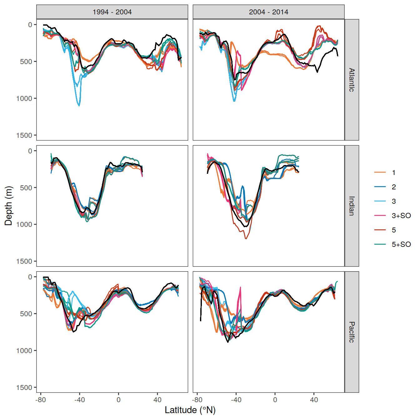
| Version | Author | Date |
|---|---|---|
| 0f2c9d5 | jens-daniel-mueller | 2022-12-08 |
| 3a7bab0 | jens-daniel-mueller | 2022-11-28 |
| 534ee74 | jens-daniel-mueller | 2022-11-25 |
| 1dad51a | jens-daniel-mueller | 2022-11-15 |
| 6edad9b | jens-daniel-mueller | 2022-11-11 |
| 16beb51 | jens-daniel-mueller | 2022-11-08 |
| b92657d | jens-daniel-mueller | 2022-11-08 |
| 7275091 | jens-daniel-mueller | 2022-11-05 |
| 99610ed | jens-daniel-mueller | 2022-11-01 |
| 7060801 | jens-daniel-mueller | 2022-10-31 |
| ecb84c1 | jens-daniel-mueller | 2022-10-30 |
| 2345935 | jens-daniel-mueller | 2022-10-29 |
| 46c163a | jens-daniel-mueller | 2022-10-10 |
| 8105380 | jens-daniel-mueller | 2022-10-07 |
# ggsave(
#   path = here::here("output/publication"),
#   filename = "FigS_dcant_penetration_depth_synthetic_data_MLR_basins.png",
#   height = 9,
#   width = 8
# )


dcant_penetration_depth_all_lat_mean_all_ensemble %>%
  filter(dcant_lim == 5,
         period %in% two_decades,
         data_source != "mod_truth") %>%
  mutate(
    data_source = case_when(
      data_source == "mod" ~ "Synthetic data",
      data_source == "obs" ~ "Observations"
    ),
    data_source = fct_reorder(data_source, desc(data_source))
  ) %>%
  ggplot(aes(
    lat,
    depth_mean,
    group = interaction(MLR_basins, Version_ID_group, data_source)
  )) +
  geom_path(aes(col = data_source)) +
  scale_colour_highcontrast() +
  labs(y = "Depth (m)",
       x = "Latitude (°N)") +
  theme(legend.title = element_blank()) +
  scale_y_reverse() +
  facet_grid(basin_AIP ~ period, scales = "free_x") +
  coord_cartesian(ylim = c(1500,0))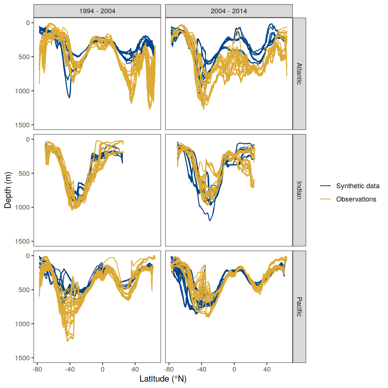
| Version | Author | Date |
|---|---|---|
| 0f2c9d5 | jens-daniel-mueller | 2022-12-08 |
| 3a7bab0 | jens-daniel-mueller | 2022-11-28 |
| 534ee74 | jens-daniel-mueller | 2022-11-25 |
| 1dad51a | jens-daniel-mueller | 2022-11-15 |
| 6edad9b | jens-daniel-mueller | 2022-11-11 |
| 16beb51 | jens-daniel-mueller | 2022-11-08 |
| b92657d | jens-daniel-mueller | 2022-11-08 |
| 7275091 | jens-daniel-mueller | 2022-11-05 |
| 99610ed | jens-daniel-mueller | 2022-11-01 |
| 7060801 | jens-daniel-mueller | 2022-10-31 |
| ecb84c1 | jens-daniel-mueller | 2022-10-30 |
| 2345935 | jens-daniel-mueller | 2022-10-29 |
| 46c163a | jens-daniel-mueller | 2022-10-10 |
# ggsave(
#   path = here::here("output/publication"),
#   filename = "FigS_dcant_penetration_depth_synthetic_data_vs_observations.png",
#   height = 9,
#   width = 8
# )

dcant_penetration_depth_all_lat_mean_all_ensemble %>%
  filter(dcant_lim == 5,
         period %in% two_decades,
         data_source == "obs") %>%
  mutate(
    data_source = case_when(
      data_source == "obs" ~ "Observations"
    ),
    data_source = fct_reorder(data_source, desc(data_source))
  ) %>%
  ggplot(aes(
    lat,
    depth_mean,
    group = interaction(MLR_basins, Version_ID_group, data_source)
  )) +
  geom_path(aes(col = MLR_basins)) +
  scale_color_vibrant() +
  labs(y = "Depth (m)",
       x = "Latitude (°N)") +
  theme(legend.title = element_blank()) +
  scale_y_reverse() +
  facet_grid(basin_AIP ~ period, scales = "free_x") +
  coord_cartesian(ylim = c(1500,0))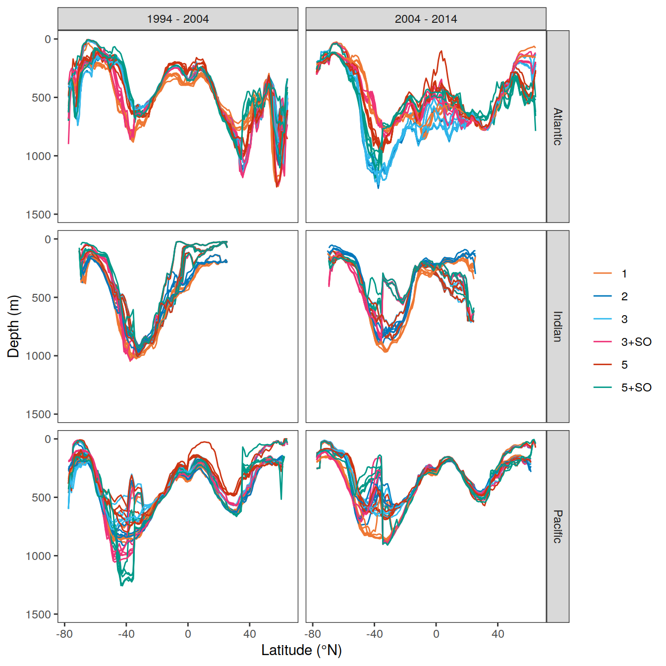
| Version | Author | Date |
|---|---|---|
| 0f2c9d5 | jens-daniel-mueller | 2022-12-08 |
| 3a7bab0 | jens-daniel-mueller | 2022-11-28 |
| 534ee74 | jens-daniel-mueller | 2022-11-25 |
| 1dad51a | jens-daniel-mueller | 2022-11-15 |
| 6edad9b | jens-daniel-mueller | 2022-11-11 |
| 16beb51 | jens-daniel-mueller | 2022-11-08 |
| b92657d | jens-daniel-mueller | 2022-11-08 |
| 7275091 | jens-daniel-mueller | 2022-11-05 |
| 99610ed | jens-daniel-mueller | 2022-11-01 |
| 7060801 | jens-daniel-mueller | 2022-10-31 |
| ecb84c1 | jens-daniel-mueller | 2022-10-30 |
| 2345935 | jens-daniel-mueller | 2022-10-29 |
| 46c163a | jens-daniel-mueller | 2022-10-10 |
13 Concentration profiles
13.1 dCant, absolute
13.1.1 Standard case
dcant_profile_basin_MLR_all %>%
  arrange(depth) %>%
  filter(period != "1994 - 2014",
         depth <= params_global$inventory_depth_standard) %>%
  group_split(data_source) %>%
  # head(1) %>%
  map(
    ~ ggplot(data = .x,
             aes(dcant,
                 depth)) +
      geom_hline(yintercept = params_global$inventory_depth_standard) +
      geom_vline(xintercept = 0) +
      geom_ribbon(
        aes(
          xmin = dcant - dcant_sd,
          xmax = dcant + dcant_sd,
          fill = period
        ),
        alpha = 0.3
      ) +
      geom_path(aes(col = period)) +
      scale_y_continuous(trans = trans_reverser("sqrt"),
                         breaks = c(0, 100, 500, seq(1500, 5000, 1000))) +
      coord_cartesian(expand = 0) +
      scale_color_brewer(
        palette = "Set1",
        name = "mean \u00B1 regional SD",
        direction = -1
      ) +
      scale_fill_brewer(
        palette = "Set1",
        name = "mean \u00B1 regional SD",
        direction = -1
      ) +
      labs(
        title = paste("data_source", unique(.x$data_source)),
        y = "Depth (m)",
        x = dcant_umol_label
      ) +
      facet_wrap( ~ basin, ncol = 3, dir = "v") +
      theme(legend.position = c(0.8, 0.2))
  )
[[1]]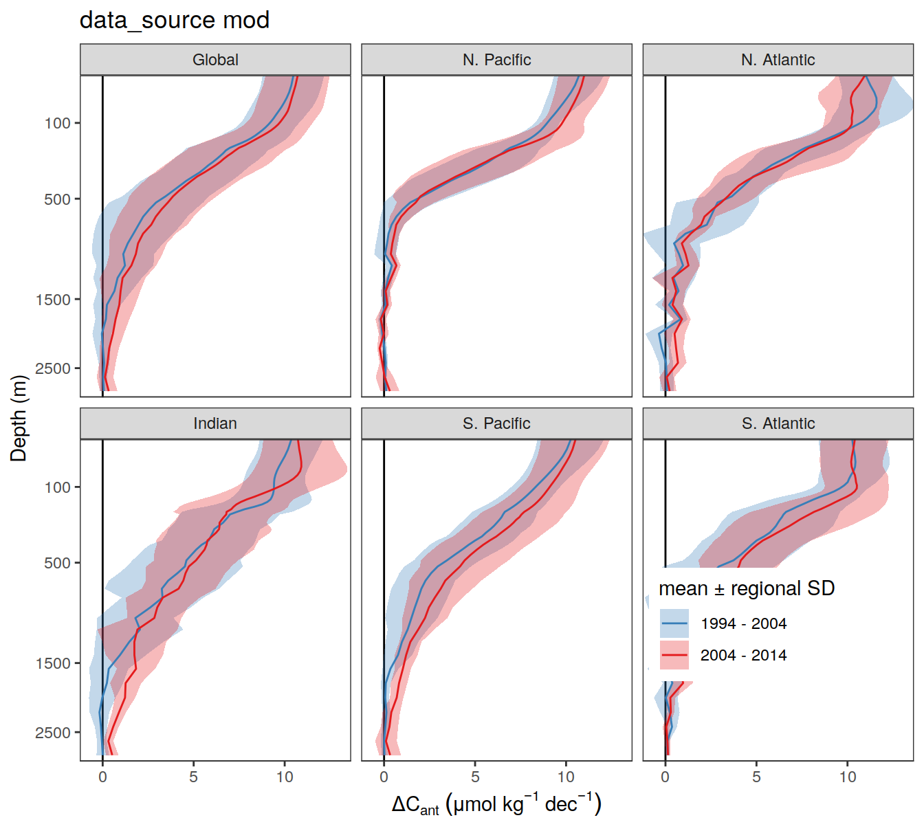
| Version | Author | Date |
|---|---|---|
| 3a7bab0 | jens-daniel-mueller | 2022-11-28 |
| 5520de8 | jens-daniel-mueller | 2022-11-15 |
| 7275091 | jens-daniel-mueller | 2022-11-05 |
| 2345935 | jens-daniel-mueller | 2022-10-29 |
| 91052ae | jens-daniel-mueller | 2022-10-20 |
| 051b911 | jens-daniel-mueller | 2022-09-07 |
| 75bd58c | jens-daniel-mueller | 2022-09-07 |
| 1c6de0d | jens-daniel-mueller | 2022-09-07 |
| 78dbb27 | jens-daniel-mueller | 2022-08-11 |
| 302d289 | jens-daniel-mueller | 2022-08-11 |
| fea41c1 | jens-daniel-mueller | 2022-07-20 |
| d2ae54c | jens-daniel-mueller | 2022-07-18 |
| 2695085 | jens-daniel-mueller | 2022-07-17 |
| 87e9eb8 | jens-daniel-mueller | 2022-06-27 |
| b52b159 | jens-daniel-mueller | 2022-06-27 |
| 1d73ec9 | jens-daniel-mueller | 2022-05-16 |
| 2ca0109 | jens-daniel-mueller | 2022-05-02 |
| b018a9a | jens-daniel-mueller | 2022-04-29 |
| e09320d | jens-daniel-mueller | 2022-04-12 |
| acad2e2 | jens-daniel-mueller | 2022-04-09 |
| 3d81135 | jens-daniel-mueller | 2022-04-07 |
| a74e341 | jens-daniel-mueller | 2022-04-04 |
| bd9e11d | jens-daniel-mueller | 2022-03-22 |
| 2501978 | jens-daniel-mueller | 2022-03-21 |
| d2191ad | jens-daniel-mueller | 2022-02-04 |
| 4673df5 | jens-daniel-mueller | 2022-02-02 |
| 60727e6 | jens-daniel-mueller | 2022-02-02 |
| 913e42f | jens-daniel-mueller | 2022-02-01 |
| 189de95 | jens-daniel-mueller | 2022-02-01 |
| b62308d | jens-daniel-mueller | 2022-01-31 |
| 5f2aed0 | jens-daniel-mueller | 2022-01-27 |
| c6fe495 | jens-daniel-mueller | 2022-01-26 |
| 9753eb8 | jens-daniel-mueller | 2022-01-26 |
| b1d7720 | jens-daniel-mueller | 2022-01-21 |
[[2]]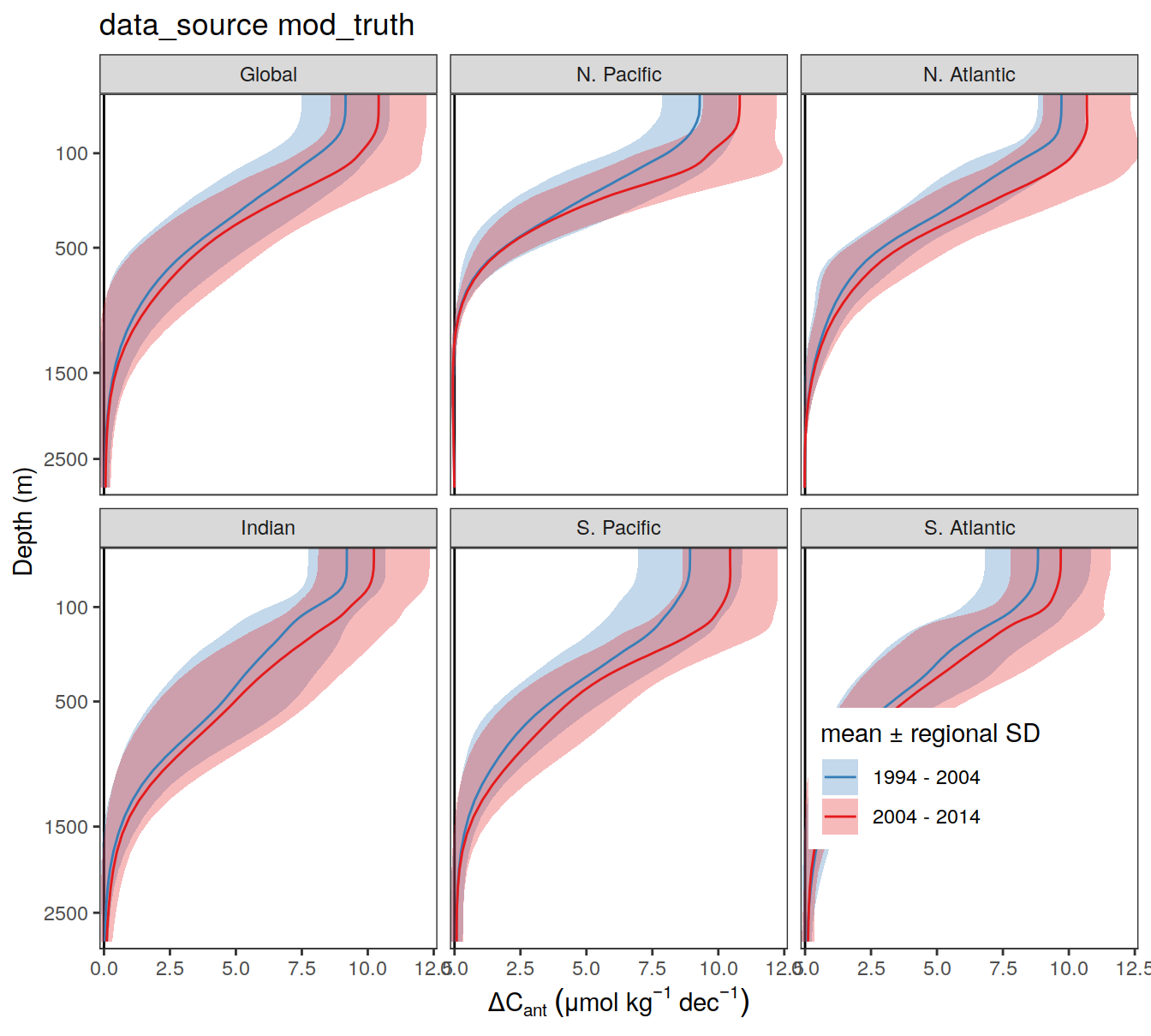
| Version | Author | Date |
|---|---|---|
| 3a7bab0 | jens-daniel-mueller | 2022-11-28 |
| 5520de8 | jens-daniel-mueller | 2022-11-15 |
| 7275091 | jens-daniel-mueller | 2022-11-05 |
| 91052ae | jens-daniel-mueller | 2022-10-20 |
| 051b911 | jens-daniel-mueller | 2022-09-07 |
| 75bd58c | jens-daniel-mueller | 2022-09-07 |
| 1c6de0d | jens-daniel-mueller | 2022-09-07 |
| 318fefe | jens-daniel-mueller | 2022-08-11 |
| fea41c1 | jens-daniel-mueller | 2022-07-20 |
| d2ae54c | jens-daniel-mueller | 2022-07-18 |
| 2695085 | jens-daniel-mueller | 2022-07-17 |
| 748aa43 | jens-daniel-mueller | 2022-06-27 |
| 16dc3af | jens-daniel-mueller | 2022-06-27 |
| 87e9eb8 | jens-daniel-mueller | 2022-06-27 |
| b52b159 | jens-daniel-mueller | 2022-06-27 |
| 1d73ec9 | jens-daniel-mueller | 2022-05-16 |
| 2ca0109 | jens-daniel-mueller | 2022-05-02 |
| b018a9a | jens-daniel-mueller | 2022-04-29 |
| e09320d | jens-daniel-mueller | 2022-04-12 |
| acad2e2 | jens-daniel-mueller | 2022-04-09 |
| 3d81135 | jens-daniel-mueller | 2022-04-07 |
| a74e341 | jens-daniel-mueller | 2022-04-04 |
| bd9e11d | jens-daniel-mueller | 2022-03-22 |
| 2501978 | jens-daniel-mueller | 2022-03-21 |
| d2191ad | jens-daniel-mueller | 2022-02-04 |
| 4673df5 | jens-daniel-mueller | 2022-02-02 |
| 60727e6 | jens-daniel-mueller | 2022-02-02 |
| 913e42f | jens-daniel-mueller | 2022-02-01 |
| 189de95 | jens-daniel-mueller | 2022-02-01 |
| b62308d | jens-daniel-mueller | 2022-01-31 |
| 5f2aed0 | jens-daniel-mueller | 2022-01-27 |
| c6fe495 | jens-daniel-mueller | 2022-01-26 |
| 9753eb8 | jens-daniel-mueller | 2022-01-26 |
| b1d7720 | jens-daniel-mueller | 2022-01-21 |
[[3]]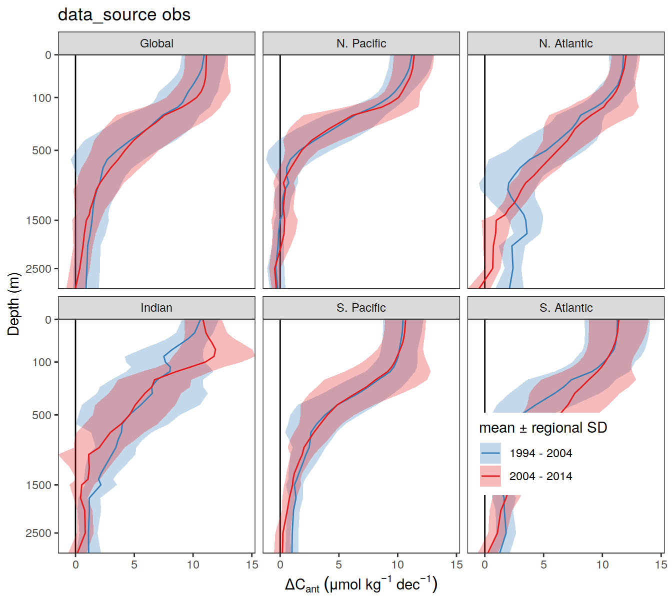
| Version | Author | Date |
|---|---|---|
| 3a7bab0 | jens-daniel-mueller | 2022-11-28 |
| 5520de8 | jens-daniel-mueller | 2022-11-15 |
| 7275091 | jens-daniel-mueller | 2022-11-05 |
| 2345935 | jens-daniel-mueller | 2022-10-29 |
| 91052ae | jens-daniel-mueller | 2022-10-20 |
| 051b911 | jens-daniel-mueller | 2022-09-07 |
| 75bd58c | jens-daniel-mueller | 2022-09-07 |
| 1c6de0d | jens-daniel-mueller | 2022-09-07 |
| 78dbb27 | jens-daniel-mueller | 2022-08-11 |
| 302d289 | jens-daniel-mueller | 2022-08-11 |
| 318fefe | jens-daniel-mueller | 2022-08-11 |
13.1.2 Ensemble members
dcant_profile_basin_MLR_all_ensemble %>%
  arrange(depth) %>%
  filter(
    period != "1994 - 2014",
    depth <= params_global$inventory_depth_standard,
    data_source == "obs"
  ) %>%
  group_split(data_source) %>%
  map(
    ~ ggplot() +
      geom_hline(yintercept = params_global$inventory_depth_standard) +
      geom_vline(xintercept = 0) +
      geom_path(
        data = .x,
        aes(
          dcant,
          depth,
          col = period,
          group = Version_ID,
          linetype = "Ensemble member",
          size = "Ensemble member",
          alpha = "Ensemble member"
        )
      ) +
      geom_path(
        data = .x %>% filter(Version_ID %in% Version_IDs),
        aes(
          dcant,
          depth,
          col = period,
          group = Version_ID,
          linetype = "Standard case",
          alpha = "Standard case",
          size = "Standard case"
        )
      ) +
      geom_path(
        data = .x %>% filter(Version_ID %in% Version_IDs),
        aes(
          dcant,
          depth,
          group = Version_ID
        )
      ) +
      scale_size_manual(values = c(0.7, 1.5), name=" ") +
      scale_linetype_manual(values = c(1, 1), name=" ") +
      scale_alpha_manual(values = c(0.4, 1), name=" ") +
      scale_y_continuous(trans = trans_reverser("sqrt"),
                         breaks = c(0, 100, 500, seq(1500, 5000, 1000))) +
      coord_cartesian(expand = 0) +
      scale_color_brewer(
        palette = "Set1",
        direction = -1
      ) +
      scale_fill_brewer(
        palette = "Set1",
        direction = -1
      ) +
      labs(
        # title = paste("data_source", unique(.x$data_source)),
        y = "Depth (m)",
        x = dcant_umol_label
      ) +
      facet_wrap( ~ basin, ncol = 3, dir = "v") +
      theme(legend.position = "top")
  )
[[1]]
| Version | Author | Date |
|---|---|---|
| 3a7bab0 | jens-daniel-mueller | 2022-11-28 |
| 534ee74 | jens-daniel-mueller | 2022-11-25 |
| 5520de8 | jens-daniel-mueller | 2022-11-15 |
| 1dad51a | jens-daniel-mueller | 2022-11-15 |
| 6edad9b | jens-daniel-mueller | 2022-11-11 |
| 16beb51 | jens-daniel-mueller | 2022-11-08 |
| b92657d | jens-daniel-mueller | 2022-11-08 |
| 7275091 | jens-daniel-mueller | 2022-11-05 |
| 99610ed | jens-daniel-mueller | 2022-11-01 |
| 7060801 | jens-daniel-mueller | 2022-10-31 |
| ecb84c1 | jens-daniel-mueller | 2022-10-30 |
| 2345935 | jens-daniel-mueller | 2022-10-29 |
| 91052ae | jens-daniel-mueller | 2022-10-20 |
| 051b911 | jens-daniel-mueller | 2022-09-07 |
| 75bd58c | jens-daniel-mueller | 2022-09-07 |
| 1c6de0d | jens-daniel-mueller | 2022-09-07 |
| 78dbb27 | jens-daniel-mueller | 2022-08-11 |
| 302d289 | jens-daniel-mueller | 2022-08-11 |
| fea41c1 | jens-daniel-mueller | 2022-07-20 |
| d2ae54c | jens-daniel-mueller | 2022-07-18 |
| 2695085 | jens-daniel-mueller | 2022-07-17 |
| 535196a | jens-daniel-mueller | 2022-07-17 |
| afb27ad | jens-daniel-mueller | 2022-07-15 |
| b492b46 | jens-daniel-mueller | 2022-07-15 |
| bd24a0f | jens-daniel-mueller | 2022-07-15 |
| f1d7f80 | jens-daniel-mueller | 2022-07-13 |
13.1.3 Surface dCant
mean_surface_dcant <- dcant_profile_basin_MLR_all_ensemble %>%
  arrange(depth) %>%
  filter(depth <= 50) %>%
  group_by(period, basin, Version_ID_group, MLR_basins, data_source) %>%
  summarise(mean_surface_dcant = mean(dcant)) %>%
  ungroup()


mean_surface_dcant %>%
  filter(period %in% two_decades,
         data_source == "obs") %>%
  ggplot(aes(x = period,
             y = mean_surface_dcant,
             fill = Version_ID_group)) +
  geom_jitter(shape = 21, alpha = 0.8) +
  scale_fill_muted() +
  facet_wrap(~basin)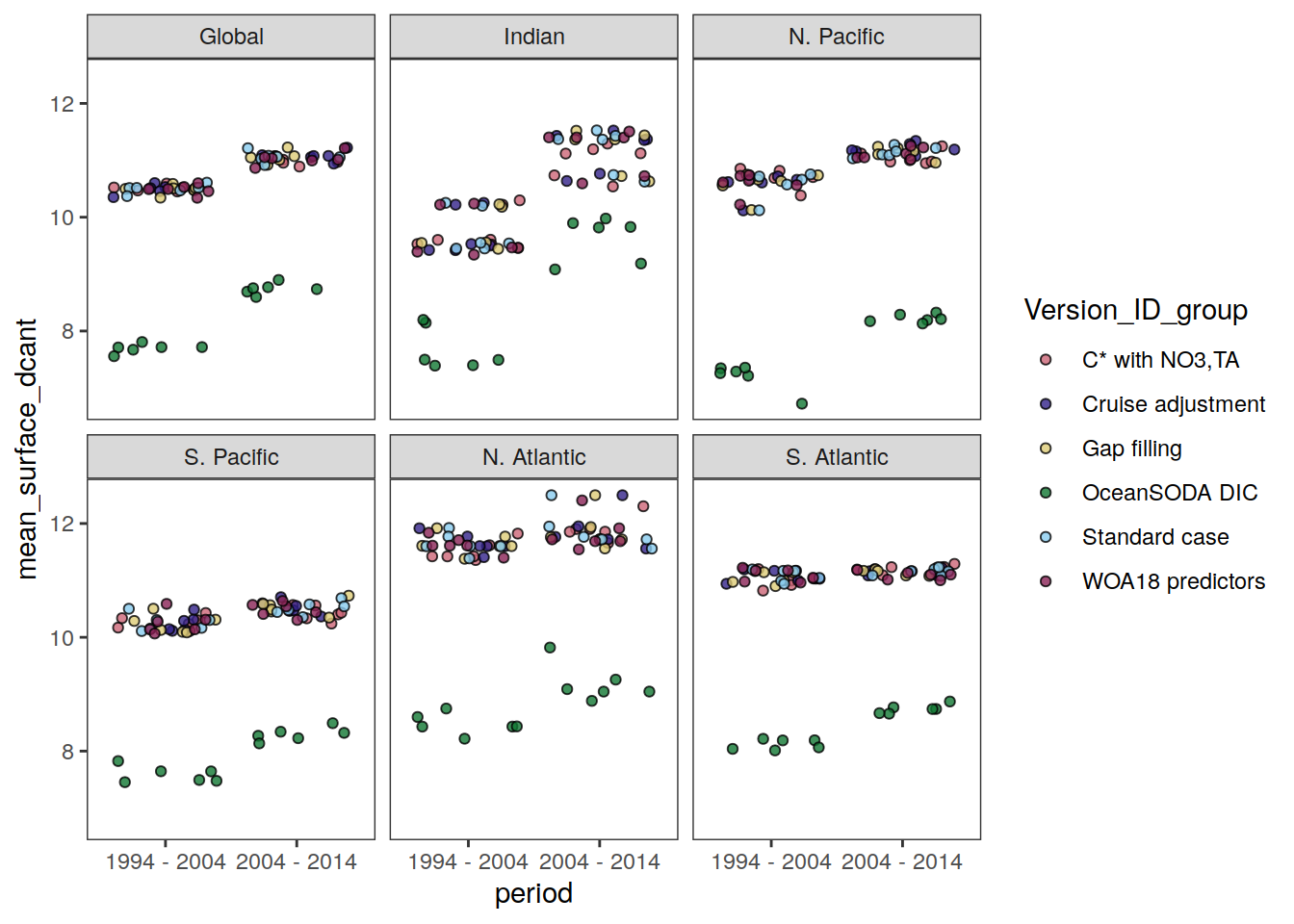
full_join(dcant_profile_basin_MLR_all_ensemble %>%
            filter(depth <= 50),
          mean_surface_dcant) %>%
  group_by(basin, period, data_source) %>%
  summarise(
    mean_surface_dcant = mean(mean_surface_dcant, na.rm = TRUE),
    sd_surface_dcant = sd(dcant) * sd_factor
  ) %>%
  ungroup() %>%
  kable() %>%
  kable_styling() %>%
scroll_box(height = "300px")| basin | period | data_source | mean_surface_dcant | sd_surface_dcant |
|---|---|---|---|---|
| Global | 1994 - 2004 | mod | 9.986285 | 1.0945634 |
| Global | 1994 - 2004 | mod_truth | 9.119623 | 0.0942101 |
| Global | 1994 - 2004 | obs | 10.027440 | 2.1875373 |
| Global | 1994 - 2014 | mod | 20.349763 | 1.7671640 |
| Global | 1994 - 2014 | mod_truth | 19.512012 | 0.1485833 |
| Global | 1994 - 2014 | obs | 20.616197 | 3.8921063 |
| Global | 2004 - 2014 | mod | 10.478444 | 0.9027755 |
| Global | 2004 - 2014 | mod_truth | 10.392390 | 0.0545695 |
| Global | 2004 - 2014 | obs | 10.657403 | 1.7478204 |
| Indian | 1994 - 2004 | mod | 9.618109 | 1.7588451 |
| Indian | 1994 - 2004 | mod_truth | 9.186885 | 0.0580122 |
| Indian | 1994 - 2004 | obs | 9.394741 | 2.2003655 |
| Indian | 1994 - 2014 | mod | 19.877479 | 3.1468737 |
| Indian | 1994 - 2014 | mod_truth | 19.386323 | 0.1379031 |
| Indian | 1994 - 2014 | obs | 20.198908 | 2.8316950 |
| Indian | 2004 - 2014 | mod | 10.400052 | 1.5129513 |
| Indian | 2004 - 2014 | mod_truth | 10.199438 | 0.0805878 |
| Indian | 2004 - 2014 | obs | 10.888760 | 1.5095440 |
| N. Pacific | 1994 - 2004 | mod | 10.098490 | 1.3675247 |
| N. Pacific | 1994 - 2004 | mod_truth | 9.221239 | 0.1727115 |
| N. Pacific | 1994 - 2004 | obs | 10.030856 | 2.7076018 |
| N. Pacific | 1994 - 2014 | mod | 20.590696 | 2.1681197 |
| N. Pacific | 1994 - 2014 | mod_truth | 19.988747 | 0.2795669 |
| N. Pacific | 1994 - 2014 | obs | 20.602712 | 4.8778119 |
| N. Pacific | 2004 - 2014 | mod | 10.518470 | 0.9349842 |
| N. Pacific | 2004 - 2014 | mod_truth | 10.767508 | 0.1072571 |
| N. Pacific | 2004 - 2014 | obs | 10.642882 | 2.2265069 |
| S. Pacific | 1994 - 2004 | mod | 9.609298 | 1.2072769 |
| S. Pacific | 1994 - 2004 | mod_truth | 8.898910 | 0.0712817 |
| S. Pacific | 1994 - 2004 | obs | 9.807174 | 2.0420842 |
| S. Pacific | 1994 - 2014 | mod | 19.847672 | 1.8235284 |
| S. Pacific | 1994 - 2014 | mod_truth | 19.346396 | 0.0775971 |
| S. Pacific | 1994 - 2014 | obs | 19.859225 | 3.6926131 |
| S. Pacific | 2004 - 2014 | mod | 10.235104 | 1.1423519 |
| S. Pacific | 2004 - 2014 | mod_truth | 10.447486 | 0.0106044 |
| S. Pacific | 2004 - 2014 | obs | 10.128636 | 1.6929087 |
| N. Atlantic | 1994 - 2004 | mod | 11.219982 | 1.1475039 |
| N. Atlantic | 1994 - 2004 | mod_truth | 9.693375 | 0.0623285 |
| N. Atlantic | 1994 - 2004 | obs | 11.093514 | 2.4026173 |
| N. Atlantic | 1994 - 2014 | mod | 21.737565 | 0.7119938 |
| N. Atlantic | 1994 - 2014 | mod_truth | 20.378481 | 0.0628299 |
| N. Atlantic | 1994 - 2014 | obs | 22.459459 | 4.4267368 |
| N. Atlantic | 2004 - 2014 | mod | 10.563675 | 1.4511103 |
| N. Atlantic | 2004 - 2014 | mod_truth | 10.685107 | 0.0125663 |
| N. Atlantic | 2004 - 2014 | obs | 11.422295 | 2.1258690 |
| S. Atlantic | 1994 - 2004 | mod | 10.109842 | 0.4621263 |
| S. Atlantic | 1994 - 2004 | mod_truth | 8.791151 | 0.0908767 |
| S. Atlantic | 1994 - 2004 | obs | 10.572092 | 2.2335592 |
| S. Atlantic | 1994 - 2014 | mod | 20.559925 | 1.2162979 |
| S. Atlantic | 1994 - 2014 | mod_truth | 18.459719 | 0.1557427 |
| S. Atlantic | 1994 - 2014 | obs | 21.288251 | 4.0332443 |
| S. Atlantic | 2004 - 2014 | mod | 10.978043 | 3.6754168 |
| S. Atlantic | 2004 - 2014 | mod_truth | 9.668568 | 0.0651916 |
| S. Atlantic | 2004 - 2014 | obs | 10.747927 | 1.8425424 |
13.1.4 Halving depth
dcant_profile_basin_MLR_all_ensemble_penetration_depth <-
full_join(dcant_profile_basin_MLR_all_ensemble,
          mean_surface_dcant) %>%
  filter(Version_ID_group != "Surface eMLR(C*)") %>%
  arrange(depth) %>%
  filter(dcant >= mean_surface_dcant / 2) %>%
  group_by(period, basin, Version_ID_group, MLR_basins, data_source) %>%
  summarise(max_depth = max(depth)) %>%
  ungroup()

dcant_profile_basin_MLR_all_ensemble_penetration_depth %>%
  filter(period %in% two_decades,
         data_source == "obs") %>%
  ggplot(aes(x = period,
             y = max_depth,
             fill = MLR_basins)) +
  geom_jitter(shape = 21, alpha = 0.8) +
  scale_fill_muted() +
  facet_wrap(~basin)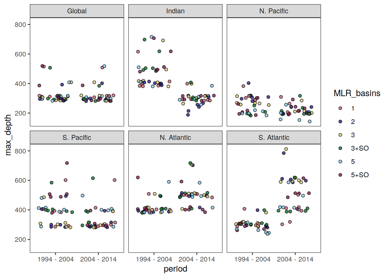
dcant_profile_basin_MLR_all_ensemble_penetration_depth_uncertainty <-
additive_uncertainty(
  dcant_profile_basin_MLR_all_ensemble_penetration_depth %>%
    rename(dcant = max_depth))

dcant_profile_basin_MLR_all_ensemble_penetration_depth_uncertainty <-
  dcant_profile_basin_MLR_all_ensemble_penetration_depth_uncertainty[[1]]

dcant_profile_basin_MLR_all_ensemble_penetration_depth_uncertainty %>%
  kable() %>%
  kable_styling() %>%
scroll_box(height = "300px")| period | basin | data_source | sd | std_case | signif_single | signif_double |
|---|---|---|---|---|---|---|
| 1994 - 2004 | Global | mod | 57.15453 | 327 | 1 | 1 |
| 1994 - 2004 | Global | mod_truth | 0.00000 | 351 | 1 | 1 |
| 1994 - 2004 | Global | obs | 100.00000 | 300 | 1 | 1 |
| 1994 - 2004 | Indian | mod | 179.17466 | 409 | 1 | 1 |
| 1994 - 2004 | Indian | mod_truth | 0.00000 | 483 | 1 | 1 |
| 1994 - 2004 | Indian | obs | 318.74755 | 400 | 1 | 0 |
| 1994 - 2004 | N. Pacific | mod | 58.37157 | 285 | 1 | 1 |
| 1994 - 2004 | N. Pacific | mod_truth | 0.00000 | 268 | 1 | 1 |
| 1994 - 2004 | N. Pacific | obs | 70.71068 | 250 | 1 | 1 |
| 1994 - 2004 | S. Pacific | mod | 79.50748 | 351 | 1 | 1 |
| 1994 - 2004 | S. Pacific | mod_truth | 0.00000 | 409 | 1 | 1 |
| 1994 - 2004 | S. Pacific | obs | 223.60680 | 300 | 1 | 0 |
| 1994 - 2004 | N. Atlantic | mod | 29.50525 | 285 | 1 | 1 |
| 1994 - 2004 | N. Atlantic | mod_truth | 0.00000 | 327 | 1 | 1 |
| 1994 - 2004 | N. Atlantic | obs | 100.00000 | 400 | 1 | 1 |
| 1994 - 2004 | S. Atlantic | mod | 31.24100 | 327 | 1 | 1 |
| 1994 - 2004 | S. Atlantic | mod_truth | 0.00000 | 351 | 1 | 1 |
| 1994 - 2004 | S. Atlantic | obs | 100.49876 | 300 | 1 | 1 |
| 1994 - 2014 | Global | mod | 54.35476 | 327 | 1 | 1 |
| 1994 - 2014 | Global | mod_truth | 0.00000 | 351 | 1 | 1 |
| 1994 - 2014 | Global | obs | 100.00000 | 300 | 1 | 1 |
| 1994 - 2014 | Indian | mod | 141.26302 | 443 | 1 | 1 |
| 1994 - 2014 | Indian | mod_truth | 0.00000 | 443 | 1 | 1 |
| 1994 - 2014 | Indian | obs | 101.98039 | 400 | 1 | 1 |
| 1994 - 2014 | N. Pacific | mod | 47.00468 | 268 | 1 | 1 |
| 1994 - 2014 | N. Pacific | mod_truth | 0.00000 | 251 | 1 | 1 |
| 1994 - 2014 | N. Pacific | obs | 113.57817 | 200 | 1 | 0 |
| 1994 - 2014 | S. Pacific | mod | 53.47560 | 378 | 1 | 1 |
| 1994 - 2014 | S. Pacific | mod_truth | 0.00000 | 409 | 1 | 1 |
| 1994 - 2014 | S. Pacific | obs | 215.40659 | 300 | 1 | 0 |
| 1994 - 2014 | N. Atlantic | mod | 25.86426 | 305 | 1 | 1 |
| 1994 - 2014 | N. Atlantic | mod_truth | 0.00000 | 351 | 1 | 1 |
| 1994 - 2014 | N. Atlantic | obs | 200.00000 | 400 | 1 | 1 |
| 1994 - 2014 | S. Atlantic | mod | 36.41758 | 327 | 1 | 1 |
| 1994 - 2014 | S. Atlantic | mod_truth | 0.00000 | 378 | 1 | 1 |
| 1994 - 2014 | S. Atlantic | obs | 153.62292 | 400 | 1 | 1 |
| 2004 - 2014 | Global | mod | 58.07753 | 327 | 1 | 1 |
| 2004 - 2014 | Global | mod_truth | 0.00000 | 351 | 1 | 1 |
| 2004 - 2014 | Global | obs | 100.00000 | 300 | 1 | 1 |
| 2004 - 2014 | Indian | mod | 175.84186 | 409 | 1 | 1 |
| 2004 - 2014 | Indian | mod_truth | 0.00000 | 443 | 1 | 1 |
| 2004 - 2014 | Indian | obs | 112.24972 | 300 | 1 | 1 |
| 2004 - 2014 | N. Pacific | mod | 38.27584 | 268 | 1 | 1 |
| 2004 - 2014 | N. Pacific | mod_truth | 0.00000 | 251 | 1 | 1 |
| 2004 - 2014 | N. Pacific | obs | 112.24972 | 200 | 1 | 0 |
| 2004 - 2014 | S. Pacific | mod | 79.52258 | 409 | 1 | 1 |
| 2004 - 2014 | S. Pacific | mod_truth | 0.00000 | 378 | 1 | 1 |
| 2004 - 2014 | S. Pacific | obs | 101.98039 | 300 | 1 | 1 |
| 2004 - 2014 | N. Atlantic | mod | 14.00000 | 327 | 1 | 1 |
| 2004 - 2014 | N. Atlantic | mod_truth | 0.00000 | 351 | 1 | 1 |
| 2004 - 2014 | N. Atlantic | obs | 224.49944 | 500 | 1 | 1 |
| 2004 - 2014 | S. Atlantic | mod | 45.00000 | 351 | 1 | 1 |
| 2004 - 2014 | S. Atlantic | mod_truth | 0.00000 | 378 | 1 | 1 |
| 2004 - 2014 | S. Atlantic | obs | 256.12497 | 600 | 1 | 1 |
dcant_profile_basin_MLR_all_ensemble_penetration_depth_uncertainty %>%
  filter(period %in% two_decades,
         data_source == "obs") %>%
  ggplot(aes(x = period,
             y = std_case,
             ymin = std_case - sd,
             ymax = std_case + sd)) +
  geom_pointrange() +
  facet_wrap(~basin)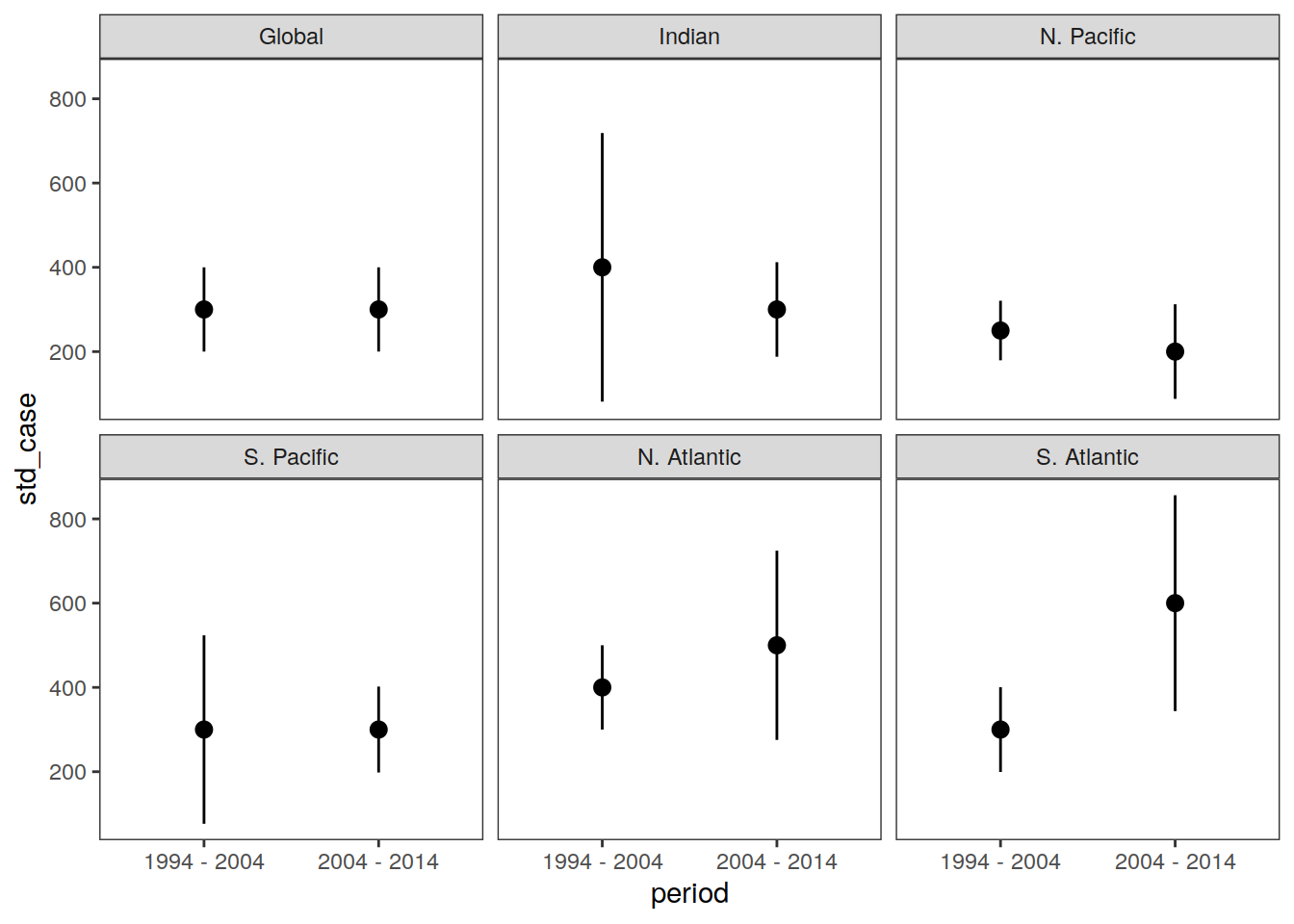
rm(dcant_profile_basin_MLR_all_ensemble_penetration_depth,
   dcant_profile_basin_MLR_all_ensemble_penetration_depth_uncertainty)
13.1.5 Additive uncertainty
# dcant_profile_basin_MLR_all_ensemble %>% distinct(data_source)

dcant_profile_basin_MLR_all_uncertainty <- dcant_profile_basin_MLR_all_ensemble %>%
  select(-c(dcant_sd, Version_ID, tref1, tref2)) %>%
  filter(period %in% two_decades)

dcant_profile_basin_MLR_all_uncertainty <- additive_uncertainty(dcant_profile_basin_MLR_all_uncertainty)

delta_dcant_profile_basin_MLR_all_uncertainty <- dcant_profile_basin_MLR_all_uncertainty[[3]]
dcant_profile_basin_MLR_all_uncertainty_contributions <- dcant_profile_basin_MLR_all_uncertainty[[2]]
dcant_profile_basin_MLR_all_uncertainty <- dcant_profile_basin_MLR_all_uncertainty[[1]]


p_dcant_profiles <-
  dcant_profile_basin_MLR_all_uncertainty %>%
  arrange(depth) %>%
  filter(
    depth <= params_global$inventory_depth_standard,
    data_source == "obs"
  ) %>%
  ggplot() +
  geom_vline(xintercept = 0, size = 0.1) +
  geom_ribbon(
    aes(
      xmin = std_case - sd*2,
      xmax = std_case + sd*2,
      y = depth,
      fill = period
    ),
    alpha = 0.2
  ) +
  geom_ribbon(
    aes(
      xmin = std_case - sd,
      xmax = std_case + sd,
      y = depth,
      fill = period
    ),
    alpha = 0.4
  ) +
  geom_path(
    aes(std_case,
        depth,
        col = period),
    size = 1
  ) +
  scale_y_reverse(breaks = seq(0,3000,500))+
  # scale_y_continuous(
  #   trans = trans_reverser("sqrt"),
  #   breaks = c(0, 100, 500, seq(1000, 5000, 1000)))+
  coord_cartesian(expand = 0, xlim = c(-2,14)) +
  scale_color_manual(values = c("#EE7733", "#009988"), name = "Mean \u00B1 1σ/2σ") +
  scale_fill_manual(values = c("#EE7733", "#009988"), name = "Mean \u00B1 1σ/2σ") +
  labs(y = "Depth (m)",
       x = dcant_umol_label) +
  facet_wrap(~ basin, ncol = 3, dir = "v") +
  theme(legend.position = c(0.9, 0.1))

p_dcant_profiles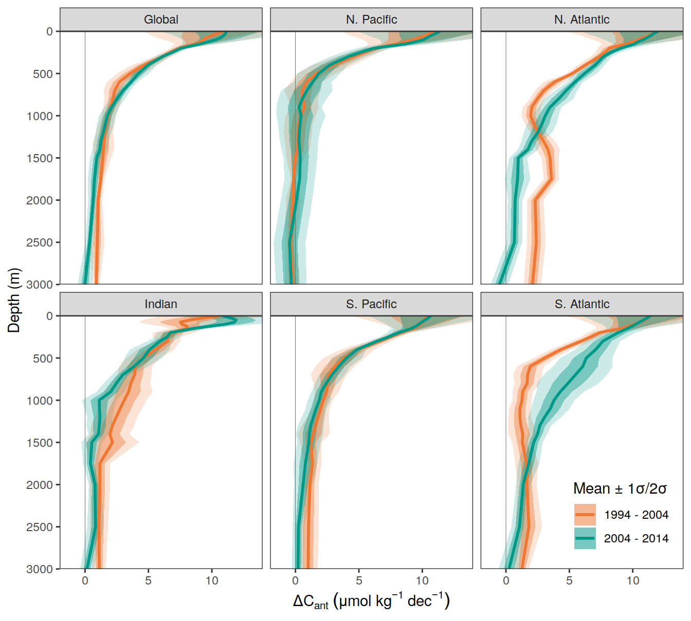
| Version | Author | Date |
|---|---|---|
| 3a7bab0 | jens-daniel-mueller | 2022-11-28 |
| 322b1c1 | jens-daniel-mueller | 2022-11-25 |
| 491f8b1 | jens-daniel-mueller | 2022-11-25 |
| 4da4d66 | jens-daniel-mueller | 2022-11-25 |
| 534ee74 | jens-daniel-mueller | 2022-11-25 |
| 5520de8 | jens-daniel-mueller | 2022-11-15 |
| 1dad51a | jens-daniel-mueller | 2022-11-15 |
| ebc85e2 | jens-daniel-mueller | 2022-11-14 |
p_dcant_profiles_mod <-
  dcant_profile_basin_MLR_all_uncertainty %>%
  arrange(depth) %>%
  filter(
    depth <= params_global$inventory_depth_standard,
    data_source != "obs"
  ) %>%
    mutate(data_source = case_when(
    data_source == "mod" ~ "Reconstruction",
    data_source == "mod_truth" ~ "Model truth"
  )) %>%
  ggplot() +
  geom_vline(xintercept = 0, size = 0.1) +
  # geom_hline(yintercept = 1000, size = 0.1) +
  geom_ribbon(
    aes(
      xmin = std_case - sd*2,
      xmax = std_case + sd*2,
      y = depth,
      fill = data_source
    ),
    alpha = 0.2
  ) +
  geom_ribbon(
    aes(
      xmin = std_case - sd,
      xmax = std_case + sd,
      y = depth,
      fill = data_source
    ),
    alpha = 0.4
  ) +
  geom_path(
    aes(std_case,
        depth,
        col = data_source),
    size = 1
  ) +
  scale_y_reverse(breaks = seq(0,3000,500)) +
  # scale_y_continuous(trans = trans_reverser("sqrt"),
  #                    breaks = c(0, 100, 500, seq(1000, 5000, 1000))) +
  coord_cartesian(expand = 0, xlim = c(-2,14)) +
  scale_color_manual(values = c("#009988", "#EE7733"), name = "Mean \u00B1 1σ/2σ") +
  scale_fill_manual(values = c("#009988", "#EE7733"), name = "Mean \u00B1 1σ/2σ") +
  labs(y = "Depth (m)",
       x = dcant_umol_label) +
  facet_grid(period ~ basin) +
  theme(legend.position = "top")

p_dcant_profiles_mod
| Version | Author | Date |
|---|---|---|
| 3a7bab0 | jens-daniel-mueller | 2022-11-28 |
| 322b1c1 | jens-daniel-mueller | 2022-11-25 |
| 491f8b1 | jens-daniel-mueller | 2022-11-25 |
| 4da4d66 | jens-daniel-mueller | 2022-11-25 |
| 534ee74 | jens-daniel-mueller | 2022-11-25 |
| 5520de8 | jens-daniel-mueller | 2022-11-15 |
| 1dad51a | jens-daniel-mueller | 2022-11-15 |
| ebc85e2 | jens-daniel-mueller | 2022-11-14 |
dcant_profile_basin_MLR_all_ensemble %>%
  arrange(depth) %>%
  filter(
    period != "1994 - 2014",
    depth <= params_global$inventory_depth_standard,
    data_source == "obs"
  ) %>%
  group_split(data_source) %>%
  map(
    ~ ggplot() +
      geom_hline(yintercept = params_global$inventory_depth_standard) +
      geom_vline(xintercept = 0) +
      geom_path(
        data = .x,
        aes(dcant,
            depth,
            col = MLR_basins,
            group = Version_ID)
      ) +
      scale_size_manual(values = c(0.5, 2), name = "x") +
      scale_linetype_manual(values = c(2, 1), name = "x") +
      scale_y_continuous(trans = trans_reverser("sqrt"),
                         breaks = c(0, 100, 500, seq(1500, 5000, 1000))) +
      coord_cartesian(expand = 0) +
      scale_color_brewer(palette = "Dark2", name = "regional\nclustering") +
      labs(y = "Depth (m)",
           x = dcant_umol_label) +
      facet_grid(basin ~ period)
  )
[[1]]
| Version | Author | Date |
|---|---|---|
| 3a7bab0 | jens-daniel-mueller | 2022-11-28 |
| 534ee74 | jens-daniel-mueller | 2022-11-25 |
| 5520de8 | jens-daniel-mueller | 2022-11-15 |
| 1dad51a | jens-daniel-mueller | 2022-11-15 |
| ebc85e2 | jens-daniel-mueller | 2022-11-14 |
| 6edad9b | jens-daniel-mueller | 2022-11-11 |
| 16beb51 | jens-daniel-mueller | 2022-11-08 |
| b92657d | jens-daniel-mueller | 2022-11-08 |
| 7275091 | jens-daniel-mueller | 2022-11-05 |
| 99610ed | jens-daniel-mueller | 2022-11-01 |
| 7060801 | jens-daniel-mueller | 2022-10-31 |
| ecb84c1 | jens-daniel-mueller | 2022-10-30 |
| 2345935 | jens-daniel-mueller | 2022-10-29 |
| 91052ae | jens-daniel-mueller | 2022-10-20 |
| 051b911 | jens-daniel-mueller | 2022-09-07 |
| 75bd58c | jens-daniel-mueller | 2022-09-07 |
| 1c6de0d | jens-daniel-mueller | 2022-09-07 |
| fea41c1 | jens-daniel-mueller | 2022-07-20 |
| d2ae54c | jens-daniel-mueller | 2022-07-18 |
| 2695085 | jens-daniel-mueller | 2022-07-17 |
| 535196a | jens-daniel-mueller | 2022-07-17 |
| afb27ad | jens-daniel-mueller | 2022-07-15 |
| b492b46 | jens-daniel-mueller | 2022-07-15 |
| bd24a0f | jens-daniel-mueller | 2022-07-15 |
| 17cd1d1 | jens-daniel-mueller | 2022-07-13 |
| 8fb595c | jens-daniel-mueller | 2022-07-12 |
| 003b161 | jens-daniel-mueller | 2022-07-12 |
| 232909e | jens-daniel-mueller | 2022-07-01 |
dcant_profile_basin_MLR_all_ensemble %>%
  arrange(depth) %>%
  filter(
    period != "1994 - 2014",
    depth <= params_global$inventory_depth_standard,
    data_source != "mod_truth"
  ) %>%
  group_split(data_source) %>%
  # head(1) %>%
  map(
    ~ ggplot() +
      geom_hline(yintercept = params_global$inventory_depth_standard) +
      geom_vline(xintercept = 0) +
      geom_path(
        data = .x,
        aes(
          dcant,
          depth,
          col = Version_ID_group,
          group = Version_ID
        )) +
      scale_y_continuous(trans = trans_reverser("sqrt"),
                         breaks = c(0, 100, 500, seq(1500, 5000, 1000))) +
      coord_cartesian(expand = 0) +
      scale_color_muted(
        name = "configuration"
      ) +
      labs(
        y = "Depth (m)",
        x = dcant_umol_label,
        title = paste("data_source", unique(.x$data_source))
      ) +
      facet_grid(basin ~ period)
  )
[[1]]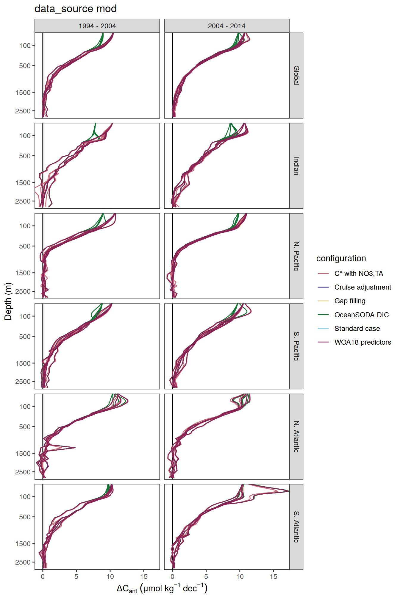
| Version | Author | Date |
|---|---|---|
| 8ded995 | jens-daniel-mueller | 2023-01-05 |
| 0f2c9d5 | jens-daniel-mueller | 2022-12-08 |
| 3a7bab0 | jens-daniel-mueller | 2022-11-28 |
| 534ee74 | jens-daniel-mueller | 2022-11-25 |
| 5520de8 | jens-daniel-mueller | 2022-11-15 |
| 1dad51a | jens-daniel-mueller | 2022-11-15 |
| ebc85e2 | jens-daniel-mueller | 2022-11-14 |
| 6edad9b | jens-daniel-mueller | 2022-11-11 |
| 16beb51 | jens-daniel-mueller | 2022-11-08 |
| b92657d | jens-daniel-mueller | 2022-11-08 |
| 7275091 | jens-daniel-mueller | 2022-11-05 |
| 99610ed | jens-daniel-mueller | 2022-11-01 |
| 7060801 | jens-daniel-mueller | 2022-10-31 |
| ecb84c1 | jens-daniel-mueller | 2022-10-30 |
| 2345935 | jens-daniel-mueller | 2022-10-29 |
| 91052ae | jens-daniel-mueller | 2022-10-20 |
| 051b911 | jens-daniel-mueller | 2022-09-07 |
| 75bd58c | jens-daniel-mueller | 2022-09-07 |
| 1c6de0d | jens-daniel-mueller | 2022-09-07 |
| fea41c1 | jens-daniel-mueller | 2022-07-20 |
| d2ae54c | jens-daniel-mueller | 2022-07-18 |
| 2695085 | jens-daniel-mueller | 2022-07-17 |
| 535196a | jens-daniel-mueller | 2022-07-17 |
| afb27ad | jens-daniel-mueller | 2022-07-15 |
| b492b46 | jens-daniel-mueller | 2022-07-15 |
| bd24a0f | jens-daniel-mueller | 2022-07-15 |
| 17cd1d1 | jens-daniel-mueller | 2022-07-13 |
| 8fb595c | jens-daniel-mueller | 2022-07-12 |
| 003b161 | jens-daniel-mueller | 2022-07-12 |
| 6be73e0 | jens-daniel-mueller | 2022-06-30 |
[[2]]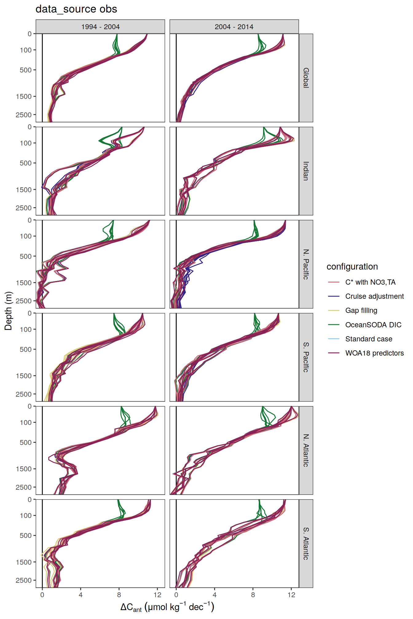
| Version | Author | Date |
|---|---|---|
| 8ded995 | jens-daniel-mueller | 2023-01-05 |
| 0f2c9d5 | jens-daniel-mueller | 2022-12-08 |
| 3a7bab0 | jens-daniel-mueller | 2022-11-28 |
| 534ee74 | jens-daniel-mueller | 2022-11-25 |
| 5520de8 | jens-daniel-mueller | 2022-11-15 |
| 1dad51a | jens-daniel-mueller | 2022-11-15 |
| ebc85e2 | jens-daniel-mueller | 2022-11-14 |
| 6edad9b | jens-daniel-mueller | 2022-11-11 |
| 16beb51 | jens-daniel-mueller | 2022-11-08 |
| b92657d | jens-daniel-mueller | 2022-11-08 |
| 7275091 | jens-daniel-mueller | 2022-11-05 |
| 91052ae | jens-daniel-mueller | 2022-10-20 |
| 051b911 | jens-daniel-mueller | 2022-09-07 |
| 75bd58c | jens-daniel-mueller | 2022-09-07 |
| 1c6de0d | jens-daniel-mueller | 2022-09-07 |
| 318fefe | jens-daniel-mueller | 2022-08-11 |
| fea41c1 | jens-daniel-mueller | 2022-07-20 |
| d2ae54c | jens-daniel-mueller | 2022-07-18 |
| 2695085 | jens-daniel-mueller | 2022-07-17 |
| 535196a | jens-daniel-mueller | 2022-07-17 |
| afb27ad | jens-daniel-mueller | 2022-07-15 |
| b492b46 | jens-daniel-mueller | 2022-07-15 |
| bd24a0f | jens-daniel-mueller | 2022-07-15 |
| 17cd1d1 | jens-daniel-mueller | 2022-07-13 |
| 8fb595c | jens-daniel-mueller | 2022-07-12 |
| 003b161 | jens-daniel-mueller | 2022-07-12 |
| 6be73e0 | jens-daniel-mueller | 2022-06-30 |
bind_rows(
  dcant_profile_basin_MLR_all_ensemble %>%
    filter(
      period %in% two_decades,
      depth <= params_global$inventory_depth_standard,
      data_source == "obs",
      Version_ID_group == "Standard case"
    ),
  dcant_profile_basin_MLR_all_sensitivity %>%
    filter(
      period %in% two_decades,
      depth <= params_global$inventory_depth_standard,
      data_source == "obs",
      Version_ID_group == "No data adjustments"
    )
) %>%
  group_by(depth,
           period,
           basin,
           Version_ID_group) %>%
  summarise(dcant_sd = sd(dcant),
            dcant = mean(dcant)) %>%
  ungroup() %>%
  filter(basin == "N. Pacific" & period == "2004 - 2014" |
         basin == "Indian" & period == "1994 - 2004") %>%
  ggplot() +
  geom_hline(yintercept = params_global$inventory_depth_standard) +
  geom_vline(xintercept = 0) +
  geom_ribbon(
    aes(
      xmin = dcant - dcant_sd*2,
      xmax = dcant + dcant_sd*2,
      y = depth,
      fill = Version_ID_group
    ),
    alpha = 0.2
  )+
  geom_ribbon(
    aes(
      xmin = dcant - dcant_sd,
      xmax = dcant + dcant_sd,
      y = depth,
      fill = Version_ID_group
    ),
    alpha = 0.4
  )+
  geom_path(aes(dcant,
                depth,
                col = Version_ID_group,
                group = Version_ID_group),
    size = 1) +
  scale_y_continuous(trans = trans_reverser("sqrt"),
                     breaks = c(0, 100, 500, seq(1500, 5000, 1000))) +
  coord_cartesian(expand = FALSE, xlim = c(-1,13)) +
  scale_color_manual(values = colour("high contrast", names = FALSE)(3)[c(1,3)],
                     name = "Mean \u00B1 1σ/2σ") +
  scale_fill_manual(values = colour("high contrast", names = FALSE)(3)[c(1,3)],
                    name = "Mean \u00B1 1σ/2σ") +
  labs(y = "Depth (m)",
       x = dcant_umol_label) +
  facet_nested_wrap(~ basin + period) +
  theme(legend.position = c(0.85,0.15))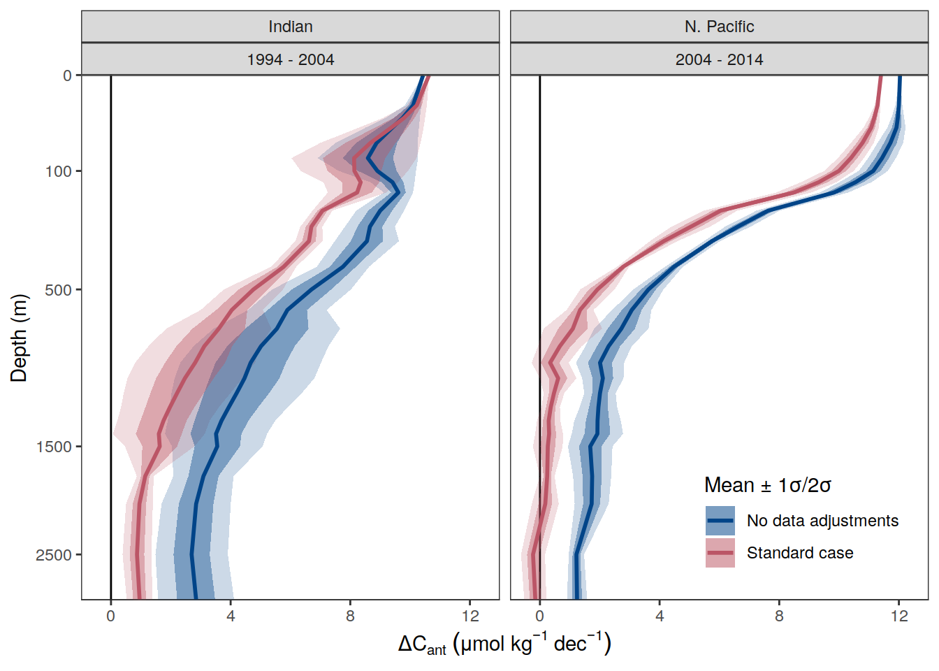
| Version | Author | Date |
|---|---|---|
| 3a7bab0 | jens-daniel-mueller | 2022-11-28 |
| 322b1c1 | jens-daniel-mueller | 2022-11-25 |
| 5520de8 | jens-daniel-mueller | 2022-11-15 |
| ebc85e2 | jens-daniel-mueller | 2022-11-14 |
| 6edad9b | jens-daniel-mueller | 2022-11-11 |
| 2345935 | jens-daniel-mueller | 2022-10-29 |
| 91052ae | jens-daniel-mueller | 2022-10-20 |
| 46c163a | jens-daniel-mueller | 2022-10-10 |
ggsave(path = here::here("output/publication"),
       filename = "FigS_dcant_profiles_data_adjustments.png",
       height = 6,
       width = 8,
       dpi = 600)
13.2 dCant - delta
delta_dcant_profile_basin_MLR_all_uncertainty %>%
  group_split(data_source) %>%
  # head(3) %>%
  map(
    ~ ggplot(data = .x,
             aes(delta_dcant,
                 depth)) +
      geom_hline(yintercept = params_global$inventory_depth_standard) +
      geom_vline(xintercept = 0) +
      geom_ribbon(
        aes(
          xmin = delta_dcant - RSS,
          xmax = delta_dcant + RSS
        ),
        alpha = 0.3
      ) +
      geom_path() +
      scale_y_continuous(trans = trans_reverser("sqrt"),
                         breaks = c(0, 100, 500, seq(1500, 5000, 1000))) +
      coord_cartesian(expand = 0) +
      scale_color_brewer(palette = "Set1", name = "mean \u00B1 sd") +
      scale_fill_brewer(palette = "Set1", name = "mean \u00B1 sd") +
      labs(
        title = paste("data_source", unique(.x$data_source)),
        y = "Depth (m)",
        x = ddcant_umol_label
      ) +
      facet_wrap(~ basin, ncol = 3)
  )
[[1]]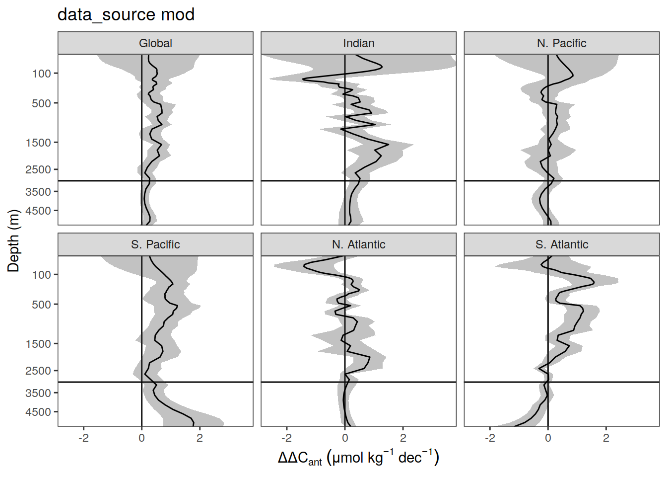
| Version | Author | Date |
|---|---|---|
| 3a7bab0 | jens-daniel-mueller | 2022-11-28 |
| 322b1c1 | jens-daniel-mueller | 2022-11-25 |
| 491f8b1 | jens-daniel-mueller | 2022-11-25 |
| 4da4d66 | jens-daniel-mueller | 2022-11-25 |
| 534ee74 | jens-daniel-mueller | 2022-11-25 |
| 5520de8 | jens-daniel-mueller | 2022-11-15 |
| 1dad51a | jens-daniel-mueller | 2022-11-15 |
| 6edad9b | jens-daniel-mueller | 2022-11-11 |
| 16beb51 | jens-daniel-mueller | 2022-11-08 |
| b92657d | jens-daniel-mueller | 2022-11-08 |
| 7275091 | jens-daniel-mueller | 2022-11-05 |
| 2345935 | jens-daniel-mueller | 2022-10-29 |
| 91052ae | jens-daniel-mueller | 2022-10-20 |
| 051b911 | jens-daniel-mueller | 2022-09-07 |
| 75bd58c | jens-daniel-mueller | 2022-09-07 |
| 1c6de0d | jens-daniel-mueller | 2022-09-07 |
| 78dbb27 | jens-daniel-mueller | 2022-08-11 |
| 302d289 | jens-daniel-mueller | 2022-08-11 |
| fea41c1 | jens-daniel-mueller | 2022-07-20 |
| d2ae54c | jens-daniel-mueller | 2022-07-18 |
| 2695085 | jens-daniel-mueller | 2022-07-17 |
| 87e9eb8 | jens-daniel-mueller | 2022-06-27 |
| b52b159 | jens-daniel-mueller | 2022-06-27 |
| 1d73ec9 | jens-daniel-mueller | 2022-05-16 |
| 2ca0109 | jens-daniel-mueller | 2022-05-02 |
| b018a9a | jens-daniel-mueller | 2022-04-29 |
| e09320d | jens-daniel-mueller | 2022-04-12 |
| acad2e2 | jens-daniel-mueller | 2022-04-09 |
| 3d81135 | jens-daniel-mueller | 2022-04-07 |
| a74e341 | jens-daniel-mueller | 2022-04-04 |
| bd9e11d | jens-daniel-mueller | 2022-03-22 |
| 2501978 | jens-daniel-mueller | 2022-03-21 |
| d2191ad | jens-daniel-mueller | 2022-02-04 |
| 913e42f | jens-daniel-mueller | 2022-02-01 |
| 189de95 | jens-daniel-mueller | 2022-02-01 |
| b62308d | jens-daniel-mueller | 2022-01-31 |
| 5f2aed0 | jens-daniel-mueller | 2022-01-27 |
| eccd82b | jens-daniel-mueller | 2022-01-26 |
| c6fe495 | jens-daniel-mueller | 2022-01-26 |
[[2]]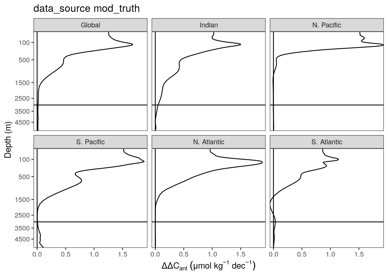
| Version | Author | Date |
|---|---|---|
| 3a7bab0 | jens-daniel-mueller | 2022-11-28 |
| 5520de8 | jens-daniel-mueller | 2022-11-15 |
| 7275091 | jens-daniel-mueller | 2022-11-05 |
| 91052ae | jens-daniel-mueller | 2022-10-20 |
| 051b911 | jens-daniel-mueller | 2022-09-07 |
| 75bd58c | jens-daniel-mueller | 2022-09-07 |
| 1c6de0d | jens-daniel-mueller | 2022-09-07 |
| 318fefe | jens-daniel-mueller | 2022-08-11 |
| fea41c1 | jens-daniel-mueller | 2022-07-20 |
| d2ae54c | jens-daniel-mueller | 2022-07-18 |
| 2695085 | jens-daniel-mueller | 2022-07-17 |
| 87e9eb8 | jens-daniel-mueller | 2022-06-27 |
| b52b159 | jens-daniel-mueller | 2022-06-27 |
| 1d73ec9 | jens-daniel-mueller | 2022-05-16 |
| 2ca0109 | jens-daniel-mueller | 2022-05-02 |
| b018a9a | jens-daniel-mueller | 2022-04-29 |
| e09320d | jens-daniel-mueller | 2022-04-12 |
| acad2e2 | jens-daniel-mueller | 2022-04-09 |
| 3d81135 | jens-daniel-mueller | 2022-04-07 |
| a74e341 | jens-daniel-mueller | 2022-04-04 |
| bd9e11d | jens-daniel-mueller | 2022-03-22 |
| 2501978 | jens-daniel-mueller | 2022-03-21 |
| d2191ad | jens-daniel-mueller | 2022-02-04 |
| 913e42f | jens-daniel-mueller | 2022-02-01 |
| 189de95 | jens-daniel-mueller | 2022-02-01 |
| b62308d | jens-daniel-mueller | 2022-01-31 |
| 5f2aed0 | jens-daniel-mueller | 2022-01-27 |
| eccd82b | jens-daniel-mueller | 2022-01-26 |
| c6fe495 | jens-daniel-mueller | 2022-01-26 |
[[3]]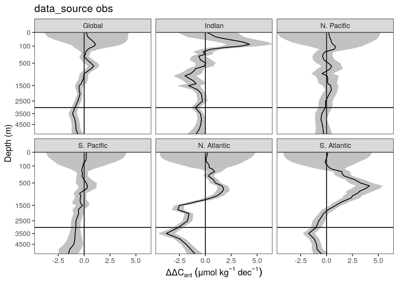
| Version | Author | Date |
|---|---|---|
| 3a7bab0 | jens-daniel-mueller | 2022-11-28 |
| 322b1c1 | jens-daniel-mueller | 2022-11-25 |
| 491f8b1 | jens-daniel-mueller | 2022-11-25 |
| 4da4d66 | jens-daniel-mueller | 2022-11-25 |
| 534ee74 | jens-daniel-mueller | 2022-11-25 |
| 5520de8 | jens-daniel-mueller | 2022-11-15 |
| 1dad51a | jens-daniel-mueller | 2022-11-15 |
| 6edad9b | jens-daniel-mueller | 2022-11-11 |
| 16beb51 | jens-daniel-mueller | 2022-11-08 |
| b92657d | jens-daniel-mueller | 2022-11-08 |
| 7275091 | jens-daniel-mueller | 2022-11-05 |
| 2345935 | jens-daniel-mueller | 2022-10-29 |
| 91052ae | jens-daniel-mueller | 2022-10-20 |
| 051b911 | jens-daniel-mueller | 2022-09-07 |
| 75bd58c | jens-daniel-mueller | 2022-09-07 |
| 1c6de0d | jens-daniel-mueller | 2022-09-07 |
| 78dbb27 | jens-daniel-mueller | 2022-08-11 |
| 302d289 | jens-daniel-mueller | 2022-08-11 |
| 318fefe | jens-daniel-mueller | 2022-08-11 |
14 Inventories
dcant_budget_basin_MLR_all_uncertainty_sensitivity <-
  dcant_budget_basin_MLR_all_sensitivity %>%
  filter(data_source != "mod_truth",
         period != "1994 - 2014") %>%
  select(-c(inv_depth, Version_ID, tref1, tref2))

dcant_budget_basin_MLR_all_uncertainty_sensitivity <- additive_uncertainty(dcant_budget_basin_MLR_all_uncertainty_sensitivity)

delta_dcant_budget_basin_MLR_all_uncertainty_sensitivity <- dcant_budget_basin_MLR_all_uncertainty_sensitivity[[3]]
dcant_budget_basin_MLR_all_uncertainty_contributions_sensitivity <- dcant_budget_basin_MLR_all_uncertainty_sensitivity[[2]]
dcant_budget_basin_MLR_all_uncertainty_sensitivity <- dcant_budget_basin_MLR_all_uncertainty_sensitivity[[1]]
dcant_budget_basin_MLR_all_uncertainty <-
dcant_budget_basin_MLR_all_ensemble %>%
filter(data_source != "mod_truth",
period == "1994 - 2014") %>%
select(-c(inv_depth, Version_ID, tref1, tref2))
dcant_budget_basin_MLR_all_uncertainty <- additive_uncertainty(dcant_budget_basin_MLR_all_uncertainty)
delta_dcant_budget_basin_MLR_all_uncertainty <- dcant_budget_basin_MLR_all_uncertainty[[3]]
dcant_budget_basin_MLR_all_uncertainty_contributions <- dcant_budget_basin_MLR_all_uncertainty[[2]]
dcant_budget_basin_MLR_all_uncertainty <- dcant_budget_basin_MLR_all_uncertainty[[1]]dcant_budget_basin_MLR_all_uncertainty <-
dcant_budget_basin_MLR_all_ensemble %>%
filter(data_source != "mod_truth",
period != "1994 - 2014") %>%
select(-c(inv_depth, Version_ID, tref1, tref2))
dcant_budget_basin_MLR_all_uncertainty <- additive_uncertainty(dcant_budget_basin_MLR_all_uncertainty)
delta_dcant_budget_basin_MLR_all_uncertainty <- dcant_budget_basin_MLR_all_uncertainty[[3]]
dcant_budget_basin_MLR_all_uncertainty_contributions <- dcant_budget_basin_MLR_all_uncertainty[[2]]
dcant_budget_basin_MLR_all_uncertainty <- dcant_budget_basin_MLR_all_uncertainty[[1]]14.1 Deep Ocean
dcant_budget_basin_MLR_all_ensemble_10000 <-
  bind_rows(
    dcant_budget_basin_MLR_all_ensemble,
    dcant_budget_basin_MLR_all_ensemble_10000)

dcant_budget_basin_MLR_all_ensemble_10000 %>%
  ggplot(aes(period,dcant, fill = as.factor(inv_depth))) +
  geom_jitter(shape = 21, alpha = 0.8) +
  facet_grid(basin ~ data_source, scales = "free_y") +
  scale_fill_highcontrast(name = "Integration\ndepth (m)") +
  scale_y_continuous(limits = c(0,NA))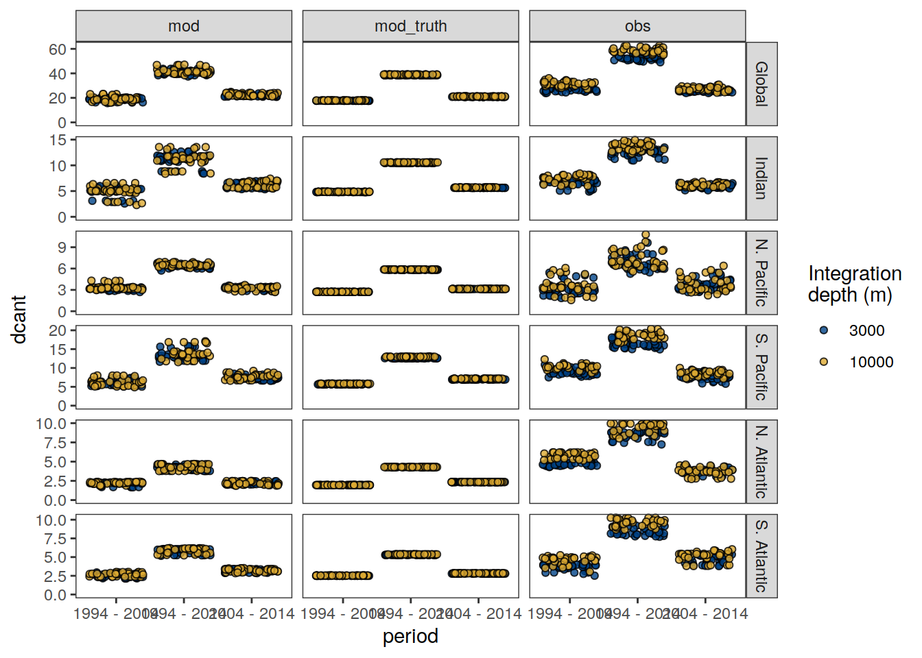
dcant_budget_basin_MLR_all_ensemble_10000 %>%
  arrange(inv_depth) %>%
  group_by(basin, period, data_source, MLR_basins, Version_ID_group) %>%
  summarise(deep_dcant = 100*((dcant / lag(dcant))-1)) %>%
  ungroup() %>%
  ggplot(aes(period,deep_dcant, fill = Version_ID_group)) +
  geom_hline(yintercept = 0) +
  geom_jitter(shape = 21, alpha = 0.8) +
  scale_fill_muted() +
  facet_grid(basin ~ data_source)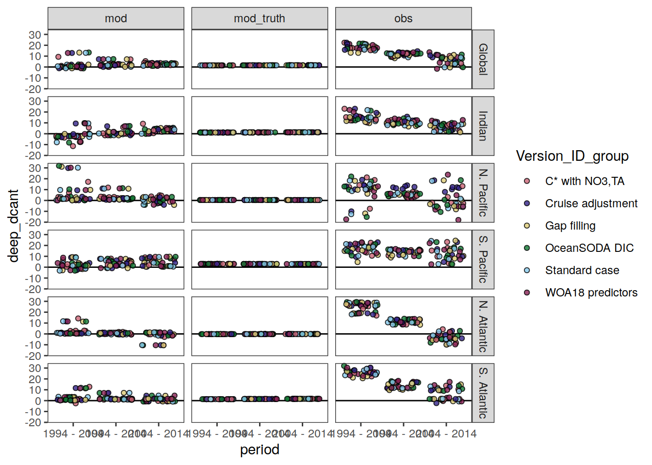
dcant_budget_basin_MLR_all_ensemble_10000 %>%
  arrange(inv_depth) %>%
  group_by(basin, period, data_source, MLR_basins, Version_ID_group) %>%
  summarise(deep_dcant = 100*((dcant / lag(dcant))-1)) %>%
  ungroup() %>%
  ggplot(aes(period,deep_dcant, fill = MLR_basins)) +
  geom_hline(yintercept = 0) +
  geom_jitter(shape = 21, alpha = 0.8) +
  scale_fill_bright() +
  facet_grid(basin ~ data_source)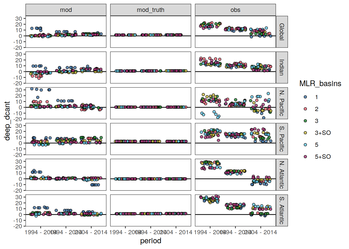
# inventory scaling

dcant_budget_basin_MLR_all_ensemble <-
  dcant_budget_basin_MLR_all_ensemble %>%
  mutate(dcant = if_else(basin == "Global",
                         dcant * dcant_scaling,
                         dcant))

dcant_budget_basin_MLR_all <- dcant_budget_basin_MLR_all %>%
  mutate(dcant = if_else(basin == "Global",
                         dcant * dcant_scaling,
                         dcant))

dcant_budget_basin_MLR_all_sensitivity <-
  dcant_budget_basin_MLR_all_sensitivity %>%
  mutate(dcant = if_else(basin == "Global",
                         dcant * dcant_scaling,
                         dcant))

# uncertainty scaling

scaling_uncertainty <-
  dcant_budget_basin_MLR_all_uncertainty %>%
  select(-c(sd, starts_with("signif_"))) %>%
  filter(basin == "Global") %>%
  mutate(
    sd = std_case * (dcant_scaling - 1) * dcant_scaling_uncertainty,
    Version_ID_group = "Scaling uncertainty"
  ) %>%
  select(-std_case)


dcant_budget_basin_MLR_all_uncertainty_contributions <-
  bind_rows(dcant_budget_basin_MLR_all_uncertainty_contributions,
            scaling_uncertainty)

rm(scaling_uncertainty)

dcant_budget_basin_MLR_all_uncertainty <-
  dcant_budget_basin_MLR_all_uncertainty %>%
  mutate(
    sd = if_else(basin == "Global",
                 sqrt(
                   sd ^ 2 +
                     (std_case * (dcant_scaling - 1) * dcant_scaling_uncertainty) ^
                     2
                 ),
                 sd),
    std_case = if_else(basin == "Global",
                       std_case * dcant_scaling,
                       std_case)
  )


dcant_budget_basin_MLR_all_uncertainty_sensitivity <-
  dcant_budget_basin_MLR_all_uncertainty_sensitivity %>%
  mutate(
    sd = if_else(basin == "Global",
                 sqrt(
                   sd ^ 2 +
                     (std_case * (dcant_scaling - 1) * dcant_scaling_uncertainty) ^
                     2
                 ),
                 sd),
    std_case = if_else(basin == "Global",
                       std_case * dcant_scaling,
                       std_case)
  )


delta_dcant_budget_basin_MLR_all_uncertainty <-
  delta_dcant_budget_basin_MLR_all_uncertainty %>%
  mutate(
    RSS = if_else(basin == "Global",
                  RSS * dcant_scaling,
                  RSS),
    delta_dcant = if_else(basin == "Global",
                          delta_dcant * dcant_scaling,
                          delta_dcant),
  )
dcant_budget_basin_MLR_all_uncertainty_contributions %>%
filter(data_source == "obs") %>%
mutate(
basin = fct_relevel(
basin,
"Global",
"N. Pacific",
"N. Atlantic",
"Indian",
"S. Pacific",
"S. Atlantic"
)
) %>%
ggplot(aes("x", abs(sd), fill = Version_ID_group)) +
geom_hline(yintercept = 0, col = "grey10") +
geom_col(position = position_dodge(preserve = "single"),
col = "grey10") +
scale_fill_bright(name = "eMLR(C*)\nconfiguration\ncomponent") +
labs(y = expression(Absolute~Delta*Cant~inventory~offset~from~standard~case~(Pg~C~dec^{-1}))) +
theme(
axis.title.x = element_blank(),
axis.text.x = element_blank(),
axis.ticks.x = element_blank()
) +
guides(pattern = guide_legend(override.aes = list(fill = "white")),
fill = guide_legend(override.aes = list(pattern = "none"))) +
# expand_limits(y = c(0,2.2)) +
# scale_y_continuous(expand = c(0,0)) +
facet_nested_wrap( ~ basin + period, ncol = 6)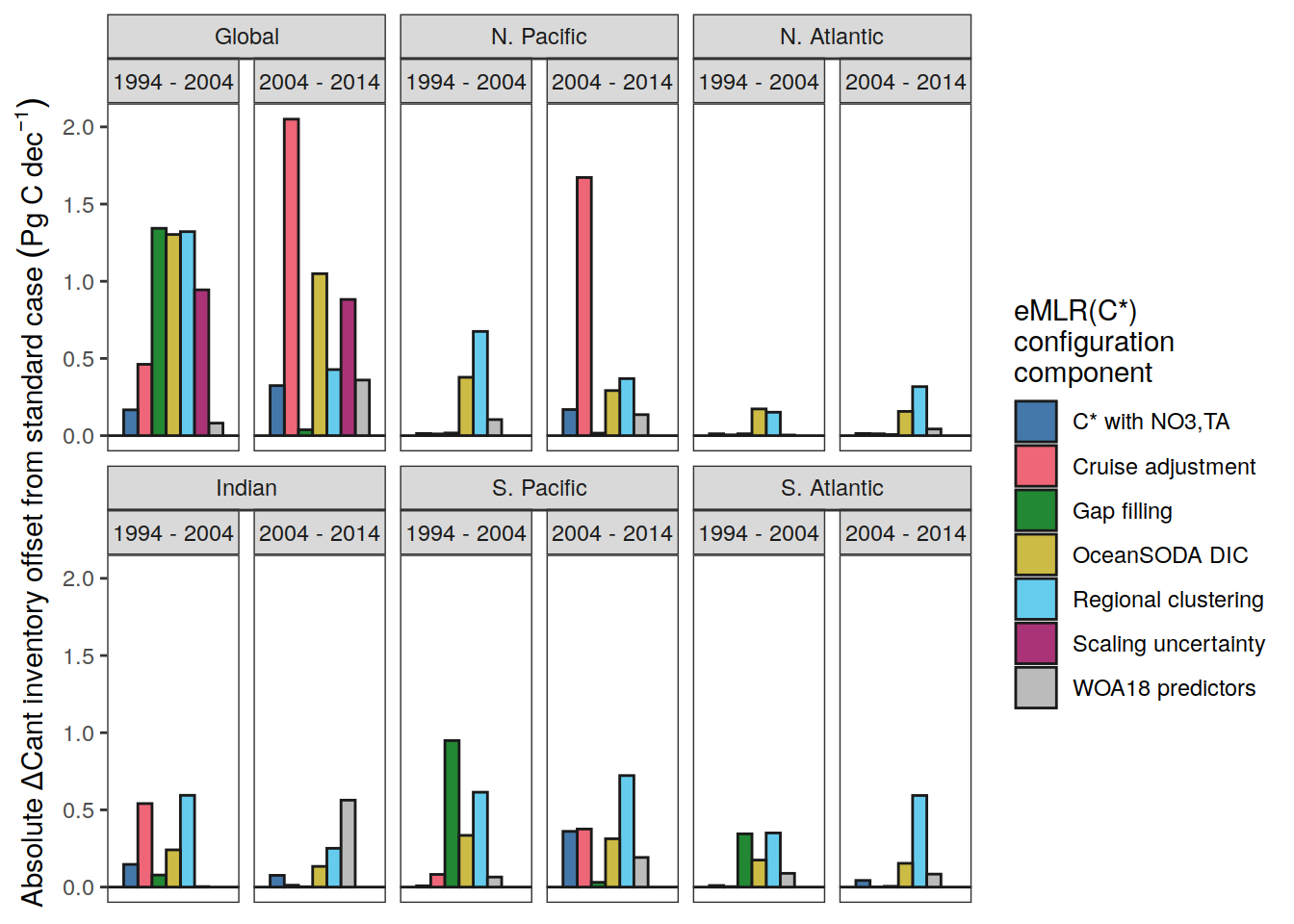
| Version | Author | Date |
|---|---|---|
| 8ded995 | jens-daniel-mueller | 2023-01-05 |
| 0f2c9d5 | jens-daniel-mueller | 2022-12-08 |
| 3a7bab0 | jens-daniel-mueller | 2022-11-28 |
| 322b1c1 | jens-daniel-mueller | 2022-11-25 |
| 491f8b1 | jens-daniel-mueller | 2022-11-25 |
| 4da4d66 | jens-daniel-mueller | 2022-11-25 |
| 534ee74 | jens-daniel-mueller | 2022-11-25 |
| f39bfd4 | jens-daniel-mueller | 2022-11-17 |
| e924c80 | jens-daniel-mueller | 2022-11-17 |
| ea34027 | jens-daniel-mueller | 2022-11-15 |
| 8ac0da0 | jens-daniel-mueller | 2022-11-15 |
| 1dad51a | jens-daniel-mueller | 2022-11-15 |
| 6edad9b | jens-daniel-mueller | 2022-11-11 |
ggsave(path = here::here("output/publication"),
       filename = "FigS_dcant_inventory_uncertainty_contributions.png",
       height = 6,
       width = 8,
       dpi = 600)
dcant_budget_basin_MLR_all_uncertainty_contributions_sensitivity %>%
filter(data_source == "obs",
Version_ID_group != "Regional clustering") %>%
mutate(
basin = fct_relevel(
basin,
"Global",
"N. Pacific",
"N. Atlantic",
"Indian",
"S. Pacific",
"S. Atlantic"
)
) %>%
ggplot(aes("x", abs(sd), fill = Version_ID_group)) +
geom_hline(yintercept = 0, col = "grey10") +
geom_col(position = position_dodge(preserve = "single"),
col = "grey10") +
scale_fill_bright(name = "eMLR(C*)\nconfiguration\ncomponent") +
labs(y = expression(Absolute~Delta*Cant~inventory~offset~from~standard~case~(Pg~C~dec^{-1}))) +
theme(
axis.title.x = element_blank(),
axis.text.x = element_blank(),
axis.ticks.x = element_blank()
) +
guides(pattern = guide_legend(override.aes = list(fill = "white")),
fill = guide_legend(override.aes = list(pattern = "none"))) +
# expand_limits(y = c(0,2.2)) +
# scale_y_continuous(expand = c(0,0)) +
facet_nested_wrap( ~ basin + period, ncol = 6)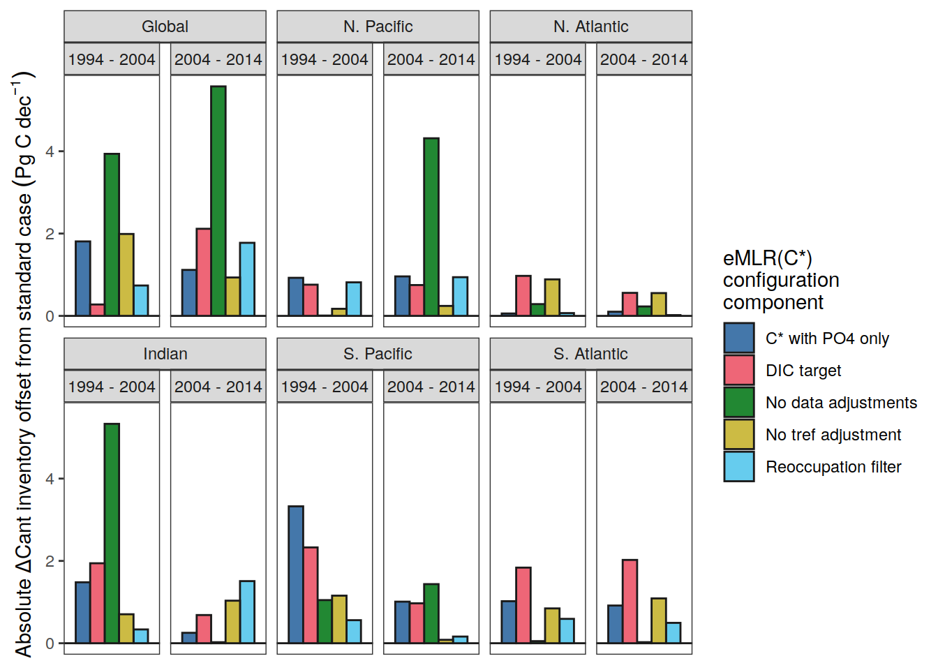
ggsave(path = here::here("output/publication"),
       filename = "FigS_dcant_inventory_uncertainty_contributions_sensitivity.png",
       height = 6,
       width = 8,
       dpi = 600)
# estimate area scaling factor to achieve identical coverage
tcant_inv <-
inner_join(tcant_inv, basinmask)
dcant_inv_all <-
inner_join(dcant_inv_all, basinmask)
area_scaling <-
bind_rows(
tcant_inv %>% distinct(lat, lon, basin) %>%
mutate(source = "SO4"),
dcant_inv_all %>% distinct(lat, lon, basin) %>%
mutate(source = "M22")
)
map +
geom_tile(data = area_scaling,
aes(lon, lat, fill = basin)) +
facet_wrap( ~ source)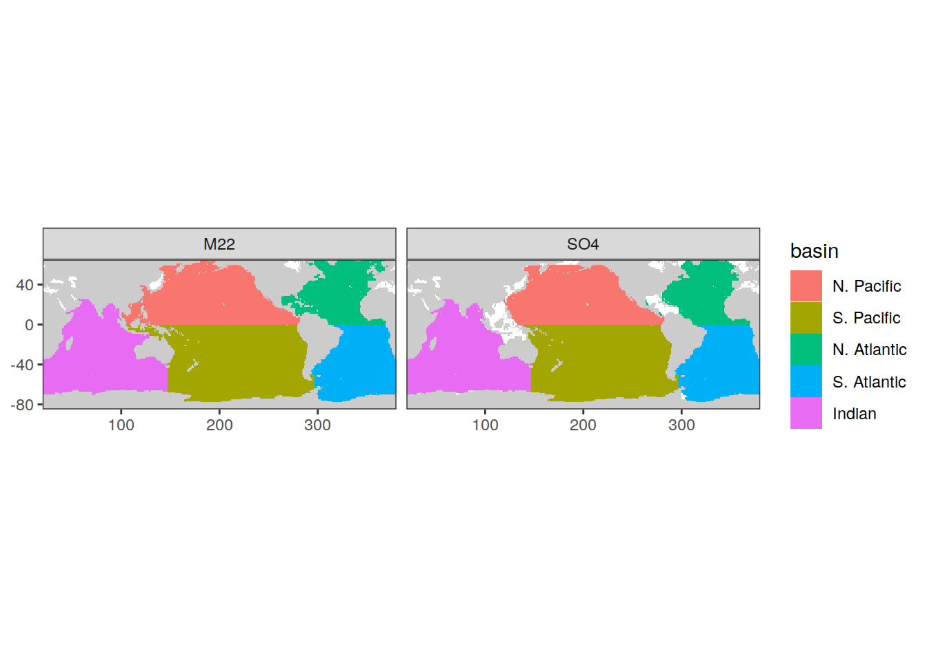
area_scaling <- area_scaling %>%
  mutate(area = earth_surf(lat, lon)) %>%
  group_by(basin, source) %>%
  summarise(area_total = sum(area)) %>%
  ungroup() %>%
  pivot_wider(values_from = area_total,
              names_from = source) %>%
  mutate(scaling_factor = M22 / SO4)


tcant_budget_basin_MLR <-
  tcant_inv %>%
  mutate(method = "layer",
         data_source = "obs") %>%
  group_by(basin) %>%
  nest() %>%
  mutate(budget = map(.x = data, ~m_dcant_budget(.x))) %>%
  select(-data) %>%
  unnest(budget)

tcant_budget_basin_MLR <-
  full_join(tcant_budget_basin_MLR,
            area_scaling %>% select(basin, scaling_factor)) %>%
  mutate(value = value * scaling_factor) %>%
  select(-scaling_factor)


tcant_budget_basin_MLR <-
  left_join(tcant_budget_basin_MLR %>%
              mutate(period = "1800 - 1994"),
            delta_pCO2_atm)


tcant_budget_basin_MLR <- tcant_budget_basin_MLR %>%
  filter(estimate == "dcant") %>%
  select(-estimate) %>%
  rename(dcant = value)

tcant_budget_basin_MLR <- tcant_budget_basin_MLR %>%
  mutate(beta_1994 = dcant / delta_pCO2) %>%
  select(basin, beta_1994)

tcant_budget_basin_MLR <-
  bind_rows(tcant_budget_basin_MLR,
            tibble(basin = "Global", beta_1994 = 118 / 78.3))
14.2 Scatterplots
14.2.1 Ensemble uncertainty
dcant_budget_basin_MLR_all_ensemble %>%
  ggplot(aes(period, dcant, col = Version_ID_group)) +
  geom_jitter(alpha = 0.5) +
  scale_color_brewer(palette = "Dark2") +
  facet_grid(basin ~ data_source, scales = "free_y")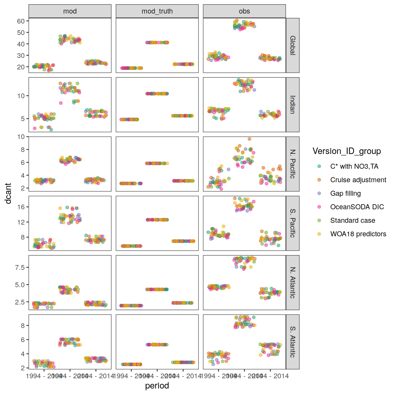
| Version | Author | Date |
|---|---|---|
| 8ded995 | jens-daniel-mueller | 2023-01-05 |
| 0f2c9d5 | jens-daniel-mueller | 2022-12-08 |
| 3a7bab0 | jens-daniel-mueller | 2022-11-28 |
| 534ee74 | jens-daniel-mueller | 2022-11-25 |
| 1dad51a | jens-daniel-mueller | 2022-11-15 |
| 6edad9b | jens-daniel-mueller | 2022-11-11 |
| 16beb51 | jens-daniel-mueller | 2022-11-08 |
| b92657d | jens-daniel-mueller | 2022-11-08 |
| 7275091 | jens-daniel-mueller | 2022-11-05 |
tcant_budget_basin_MLR <- expand_grid(
  tcant_budget_basin_MLR,
  delta_pCO2_atm %>% filter(period %in% two_decades)
)

tcant_budget_basin_MLR <- tcant_budget_basin_MLR %>%
  mutate(dcant = beta_1994 * delta_pCO2)

tcant_budget_basin_MLR <- tcant_budget_basin_MLR %>%
  mutate(
    basin = fct_relevel(
      basin,
      "Global",
      "Indian",
      "N. Pacific",
      "S. Pacific",
      "N. Atlantic",
      "S. Atlantic"
    )
  )


dcant_budget_basin_MLR_all_ensemble %>%
  filter(data_source == "obs",
         period != "1994 - 2014") %>%
  mutate(ensemble_role = "Uncertainty cases") %>%
  ggplot(aes(period, dcant)) +
  # scale_fill_muted(name = "ensemble group") +
  scale_color_manual(values = c("grey", "black", "red"),
                     name = "Ensemble member") +
  geom_boxplot(
    width = .1,
    outlier.shape = NA,
    fill = "grey",
    alpha = 0.7,
    position = position_nudge(x = 0.3)
  ) +
  geom_point(
    data = dcant_budget_basin_MLR_all_sensitivity %>%
      mutate(ensemble_role = "Sensitivity cases") %>%
      filter(data_source == "obs",
         period != "1994 - 2014"),
    aes(fill = Version_ID_group,
        col = ensemble_role),
    size = 1.3,
    alpha = .7,
    shape = 21,
    position = position_dodge2(width = 0.3)
  ) +
  geom_point(
    aes(fill = Version_ID_group,
        col = ensemble_role),
    size = 1.3,
    alpha = .7,
    shape = 21,
    position = position_dodge2(width = 0.3)
  ) +
  scale_y_continuous(name = dcant_pgc_label) +
  facet_wrap(~ basin, ncol = 3, scales = "free_y")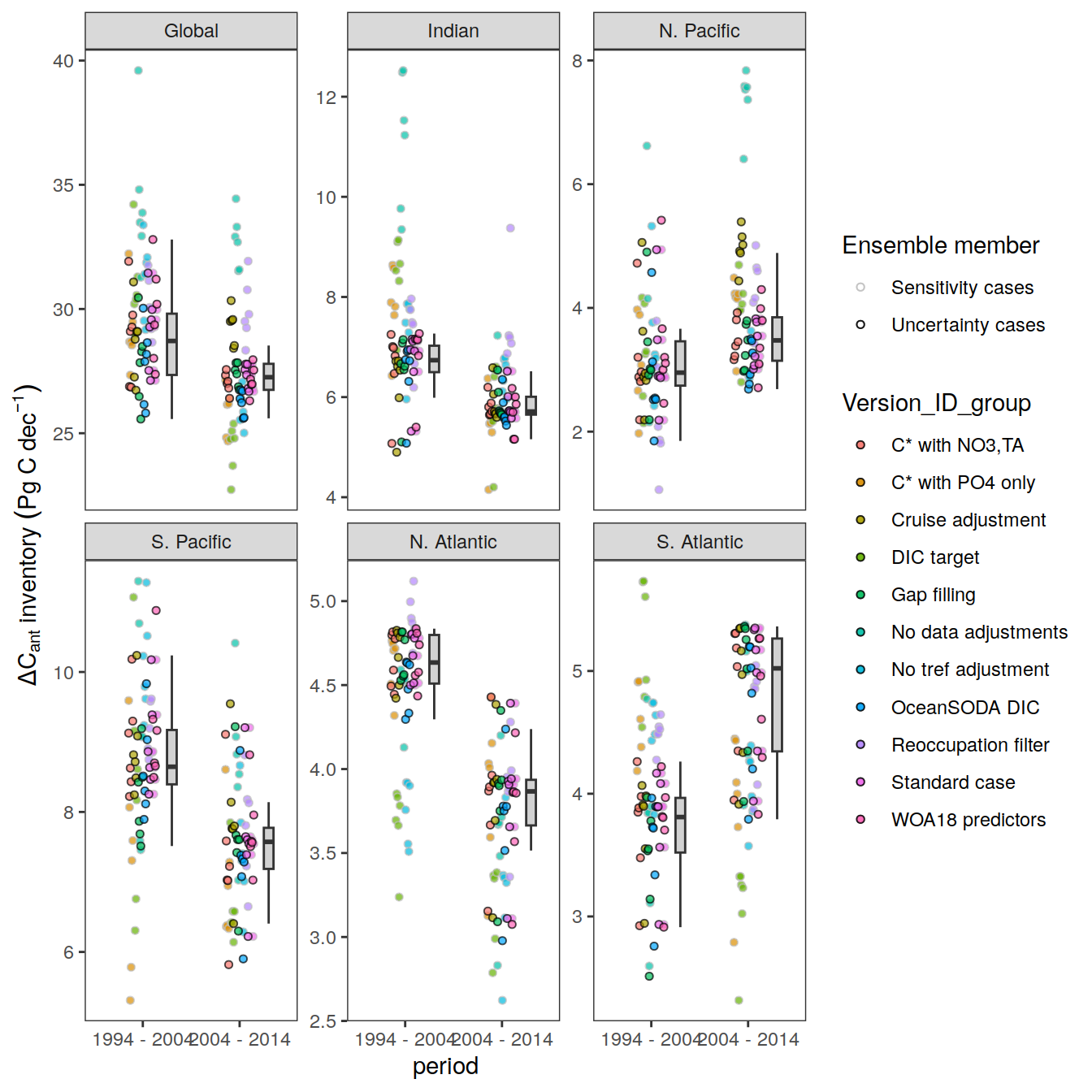
| Version | Author | Date |
|---|---|---|
| 8ded995 | jens-daniel-mueller | 2023-01-05 |
| 0f2c9d5 | jens-daniel-mueller | 2022-12-08 |
| 3a7bab0 | jens-daniel-mueller | 2022-11-28 |
| 534ee74 | jens-daniel-mueller | 2022-11-25 |
| ea34027 | jens-daniel-mueller | 2022-11-15 |
| 5520de8 | jens-daniel-mueller | 2022-11-15 |
| 1dad51a | jens-daniel-mueller | 2022-11-15 |
| 375300e | jens-daniel-mueller | 2022-11-14 |
| ebc85e2 | jens-daniel-mueller | 2022-11-14 |
| 6edad9b | jens-daniel-mueller | 2022-11-11 |
| 16beb51 | jens-daniel-mueller | 2022-11-08 |
| b92657d | jens-daniel-mueller | 2022-11-08 |
| 7275091 | jens-daniel-mueller | 2022-11-05 |
14.2.2 Additive uncertainty
dcant_budget_basin_MLR_all_ensemble %>%
  filter(data_source == "obs",
         period != "1994 - 2014",
         !(Version_ID %in% Version_IDs),
         MLR_basins == unique(params_local_all$MLR_basins)) %>%
  ggplot(aes(period, dcant)) +
  geom_errorbar(
    data = tcant_budget_basin_MLR,
    aes(x = period,
        ymax = dcant, ymin = dcant,
        col = "Scaled 1994\nestimate"),
    width = 0.8,
    size = 1,
    linetype = 1,
    position = position_nudge(x = 0.05)
  ) +
  geom_jitter(
    data = dcant_budget_basin_MLR_all_ensemble %>%
      filter(data_source == "obs",
             period != "1994 - 2014",
             Version_ID_group == unique(params_local_all$Version_ID_group)),
    aes(fill = "Regional clustering",
        alpha = "Regional clustering"),
    shape = 21,
    position = position_jitter(width = 0.1, height = 0)
  ) +
  geom_point(
    aes(fill = "Configuration changes",
        alpha = "Configuration changes"),
    shape = 21,
    position = position_jitter(width = 0.1, height = 0)
  ) +
  geom_crossbar(
    data = dcant_budget_basin_MLR_all_uncertainty %>% filter(data_source == "obs"),
    aes(
      x = period,
      y = std_case,
      ymin = std_case - sd*2,
      ymax = std_case + sd*2,
      linetype = "Combined uncertainty"
    ),
    width = 0.1,
    fill = "#BBBBBB",
    alpha = 0.2,
    position = position_nudge(x = 0.2)
  ) +
  geom_crossbar(
    data = dcant_budget_basin_MLR_all_uncertainty %>% filter(data_source == "obs"),
    aes(
      x = period,
      y = std_case,
      ymin = std_case - sd,
      ymax = std_case + sd,
      alpha = "Combined uncertainty",
    ),
    width = 0.1,
    fill = "#BBBBBB",
    alpha = 0.4,
    position = position_nudge(x = 0.2)
  ) +
  geom_point(
    data = dcant_budget_basin_MLR_all_uncertainty %>% filter(data_source == "obs"),
    aes(x = period,
        y = std_case,
        fill = "Standard case",
        alpha = "Standard case"),
    size = 2,
    shape = 21,
    position = position_nudge(x = 0.2)
  ) +
  scale_fill_manual(name = "group", values = c("#BB5566", "#004488", "white")) +
  scale_color_manual(values = c("grey50"), label = expression(Scaled~C[ant]~1994)) +
  scale_linetype(name = "X") +
  scale_alpha_manual(name = "group", values = c(0.7,0.7,1)) +
  scale_shape_manual(values = 95) +
  scale_y_continuous(name = dcant_pgc_label) +
  guides(
    fill = guide_legend(order = 1),
    linetype = guide_legend(order = 2),
    alpha = guide_legend(order = 1)
  ) +
  facet_wrap(~ basin, ncol = 3, dir = "v", scales = "free_y") +
  theme(legend.title = element_blank(),
        axis.title.x = element_blank())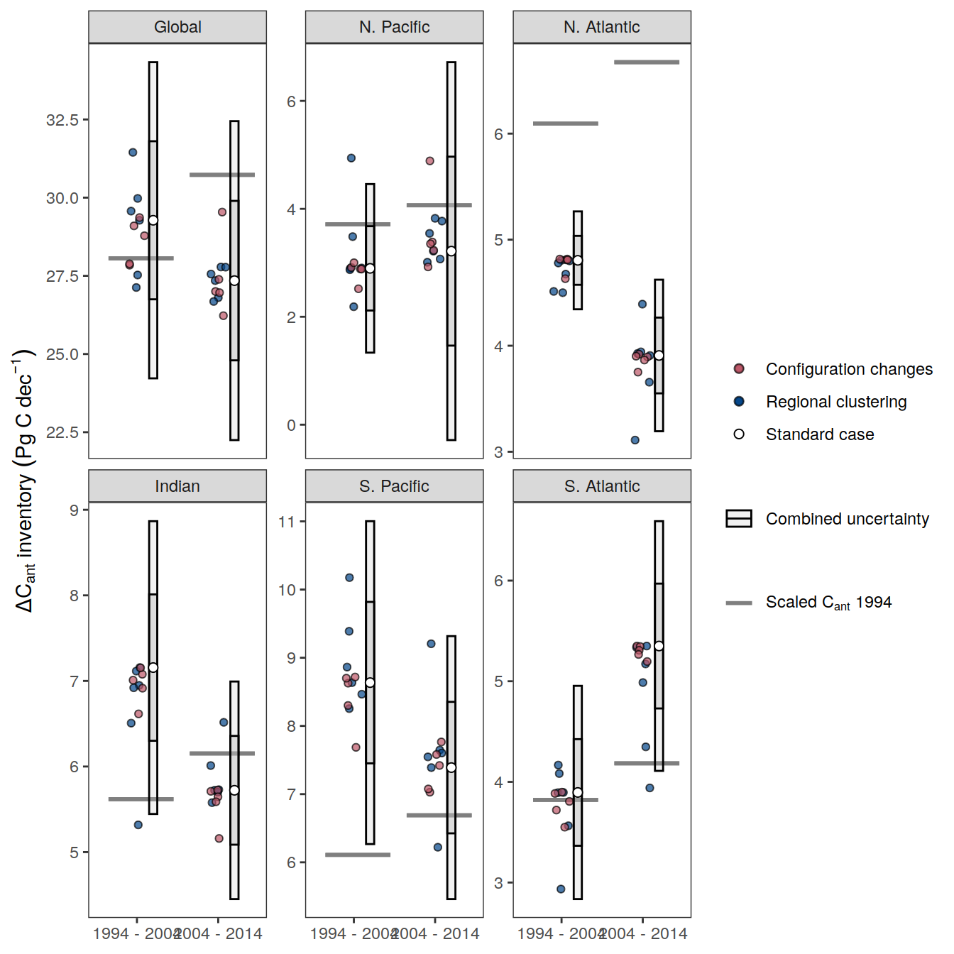
| Version | Author | Date |
|---|---|---|
| 0f2c9d5 | jens-daniel-mueller | 2022-12-08 |
| 3a7bab0 | jens-daniel-mueller | 2022-11-28 |
| 322b1c1 | jens-daniel-mueller | 2022-11-25 |
| 491f8b1 | jens-daniel-mueller | 2022-11-25 |
| 4da4d66 | jens-daniel-mueller | 2022-11-25 |
| 534ee74 | jens-daniel-mueller | 2022-11-25 |
| e924c80 | jens-daniel-mueller | 2022-11-17 |
| ea34027 | jens-daniel-mueller | 2022-11-15 |
| 5520de8 | jens-daniel-mueller | 2022-11-15 |
| 1dad51a | jens-daniel-mueller | 2022-11-15 |
| ebc85e2 | jens-daniel-mueller | 2022-11-14 |
| 6edad9b | jens-daniel-mueller | 2022-11-11 |
| 16beb51 | jens-daniel-mueller | 2022-11-08 |
| b92657d | jens-daniel-mueller | 2022-11-08 |
| 0b939ca | jens-daniel-mueller | 2022-11-08 |
| 7275091 | jens-daniel-mueller | 2022-11-05 |
ggsave(path = here::here("output/publication"),
       filename = "Fig_dcant_inventory.png",
       height = 6,
       width = 8,
       dpi = 600)
14.2.3 Beta
# determine scaling factor from dcant -> beta inventories
# including scaling for: delta pCO2 atm, basin area, PgC -> molC

beta_scaling <-
  bind_rows(
    area_scaling,
    area_scaling %>%
      summarise(M22 = sum(M22) * dcant_scaling) %>%
      mutate(basin = "Global")
  ) %>%
  select(basin, area = M22)


beta_scaling <-
  full_join(delta_pCO2_atm,
            beta_scaling,
            by = character())

beta_scaling <- beta_scaling %>%
  mutate(scaling_factor = 1e15 / 12 / delta_pCO2 / area) %>%
  select(period, basin, scaling_factor, area)

beta_scaling <- beta_scaling %>%
  mutate(
    basin = fct_relevel(
      basin,
      "Global",
      "Indian",
      "N. Pacific",
      "S. Pacific",
      "N. Atlantic",
      "S. Atlantic"
    )
  )

beta_budget_basin_MLR_all_sensitivity <-
  left_join(dcant_budget_basin_MLR_all_sensitivity,
            beta_scaling) %>%
  mutate(beta = dcant * scaling_factor) %>%
  select(-scaling_factor)

beta_budget_basin_MLR_all_ensemble <-
  left_join(dcant_budget_basin_MLR_all_ensemble,
            beta_scaling) %>%
  mutate(beta = dcant * scaling_factor) %>%
  select(-scaling_factor)


tcant_budget_basin_MLR <-
  left_join(tcant_budget_basin_MLR,
            beta_scaling) %>%
  mutate(beta_1994 = beta_1994 * 1e15 / 12 / area) %>%
  select(-c(area,scaling_factor))

beta_budget_basin_MLR_all_uncertainty <-
  left_join(dcant_budget_basin_MLR_all_uncertainty,
            beta_scaling) %>%
  mutate(
    sd = sd * scaling_factor,
    std_case = std_case * scaling_factor
    ) %>%
  select(-scaling_factor)

beta_budget_basin_MLR_all_uncertainty_contributions <-
  left_join(dcant_budget_basin_MLR_all_uncertainty_contributions,
            beta_scaling) %>%
  mutate(
    sd = sd * scaling_factor
    ) %>%
  select(-scaling_factor)
dcant_beta_basin_MLR_all_uncertainty <-
bind_rows(
dcant_budget_basin_MLR_all_uncertainty %>% mutate(estimate = "dcant"),
beta_budget_basin_MLR_all_uncertainty %>% mutate(estimate = "beta")
) %>%
select(-c(area, starts_with("signif_")))
dcant_beta_basin_MLR_all_uncertainty_significance <-
dcant_beta_basin_MLR_all_uncertainty %>%
arrange(period) %>%
group_by(estimate, basin, data_source) %>%
mutate(
delta = std_case - lag(std_case),
RSS = sqrt(sd ^ 2 + lag(sd ^ 2))
) %>%
ungroup() %>%
filter(!is.na(delta))
dcant_beta_basin_MLR_all_uncertainty_significance <-
full_join(
dcant_beta_basin_MLR_all_uncertainty %>%
pivot_wider(
names_from = period,
values_from = c(sd, std_case),
names_sep = " "
),
dcant_beta_basin_MLR_all_uncertainty_significance %>%
select(-c(sd, std_case))
)
dcant_beta_basin_MLR_all_uncertainty_significance <-
dcant_beta_basin_MLR_all_uncertainty_significance %>%
mutate(across(where(is.numeric), signif, 2))
dcant_beta_basin_MLR_all_uncertainty_significance %>%
kable() %>%
kable_styling() %>%
scroll_box(height = "300px")| basin | data_source | estimate | sd 1994 - 2004 | sd 2004 - 2014 | std_case 1994 - 2004 | std_case 2004 - 2014 | period | delta | RSS |
|---|---|---|---|---|---|---|---|---|---|
| Global | mod | dcant | 1.600 | 1.600 | 20.00 | 25.00 | 2004 - 2014 | 4.8000 | 2.300 |
| Global | obs | dcant | 2.500 | 2.500 | 29.00 | 27.00 | 2004 - 2014 | -1.9000 | 3.600 |
| Indian | mod | dcant | 0.800 | 0.700 | 5.10 | 6.60 | 2004 - 2014 | 1.5000 | 1.100 |
| Indian | obs | dcant | 0.860 | 0.640 | 7.20 | 5.70 | 2004 - 2014 | -1.4000 | 1.100 |
| N. Pacific | mod | dcant | 0.260 | 0.300 | 3.10 | 3.40 | 2004 - 2014 | 0.2300 | 0.400 |
| N. Pacific | obs | dcant | 0.780 | 1.800 | 2.90 | 3.20 | 2004 - 2014 | 0.3200 | 1.900 |
| S. Pacific | mod | dcant | 0.800 | 0.440 | 5.50 | 7.40 | 2004 - 2014 | 1.9000 | 0.920 |
| S. Pacific | obs | dcant | 1.200 | 0.960 | 8.60 | 7.40 | 2004 - 2014 | -1.2000 | 1.500 |
| N. Atlantic | mod | dcant | 0.180 | 0.280 | 2.20 | 2.40 | 2004 - 2014 | 0.2200 | 0.330 |
| N. Atlantic | obs | dcant | 0.230 | 0.360 | 4.80 | 3.90 | 2004 - 2014 | -0.9000 | 0.430 |
| S. Atlantic | mod | dcant | 0.230 | 0.240 | 2.70 | 3.40 | 2004 - 2014 | 0.7100 | 0.330 |
| S. Atlantic | obs | dcant | 0.530 | 0.620 | 3.90 | 5.40 | 2004 - 2014 | 1.5000 | 0.820 |
| Global | mod | beta | 0.020 | 0.018 | 0.25 | 0.28 | 2004 - 2014 | 0.0340 | 0.027 |
| Global | obs | beta | 0.032 | 0.029 | 0.37 | 0.31 | 2004 - 2014 | -0.0540 | 0.043 |
| Indian | mod | beta | 0.049 | 0.039 | 0.31 | 0.37 | 2004 - 2014 | 0.0540 | 0.063 |
| Indian | obs | beta | 0.052 | 0.036 | 0.44 | 0.32 | 2004 - 2014 | -0.1200 | 0.063 |
| N. Pacific | mod | beta | 0.015 | 0.016 | 0.18 | 0.18 | 2004 - 2014 | -0.0033 | 0.022 |
| N. Pacific | obs | beta | 0.045 | 0.091 | 0.17 | 0.17 | 2004 - 2014 | 0.0023 | 0.100 |
| S. Pacific | mod | beta | 0.037 | 0.019 | 0.26 | 0.32 | 2004 - 2014 | 0.0580 | 0.042 |
| S. Pacific | obs | beta | 0.055 | 0.041 | 0.40 | 0.31 | 2004 - 2014 | -0.0880 | 0.069 |
| N. Atlantic | mod | beta | 0.020 | 0.028 | 0.24 | 0.25 | 2004 - 2014 | 0.0010 | 0.034 |
| N. Atlantic | obs | beta | 0.025 | 0.036 | 0.53 | 0.39 | 2004 - 2014 | -0.1400 | 0.044 |
| S. Atlantic | mod | beta | 0.023 | 0.022 | 0.27 | 0.31 | 2004 - 2014 | 0.0410 | 0.032 |
| S. Atlantic | obs | beta | 0.053 | 0.057 | 0.39 | 0.49 | 2004 - 2014 | 0.0990 | 0.078 |
dcant_beta_basin_MLR_all_uncertainty_significance_table <-
dcant_beta_basin_MLR_all_uncertainty_significance %>%
  filter(data_source == "obs") %>%
  select(-data_source) %>%
  mutate(
    `1994 - 2004` = paste(`std_case 1994 - 2004`, `sd 1994 - 2004`, sep = " ± "),
    `2004 - 2014` = paste(`std_case 2004 - 2014`, `sd 2004 - 2014`, sep = " ± "),
    `Decadal change` = paste0(delta, " ± ", RSS,
                              if_else(abs(delta) > RSS, " *",""),
                              if_else(abs(delta) > RSS*2, "*",""))
  ) %>%
  select(Region = basin,
         Estimate = estimate,
         `1994 - 2004`,
         `2004 - 2014`,
         `Decadal change`) %>%
  arrange(Region)

dcant_beta_basin_MLR_all_uncertainty_significance_table %>%
  write_csv(here::here("output/publication/Table_inventory_stats.csv"))
beta_budget_basin_MLR_all_ensemble %>%
filter(
data_source == "obs",
period != "1994 - 2014",
!(Version_ID %in% Version_IDs),
MLR_basins == unique(params_local_all$MLR_basins)
) %>%
ggplot(aes(period, beta)) +
geom_errorbar(
data = tcant_budget_basin_MLR %>%
rename(beta = beta_1994),
aes(x = period,
ymax = beta, ymin = beta,
col = "Scaled 1994\nestimate"),
width = 0.8,
size = 1,
linetype = 1,
position = position_nudge(x = 0.05)
) +
geom_jitter(
data = beta_budget_basin_MLR_all_ensemble %>%
filter(data_source == "obs",
period != "1994 - 2014",
Version_ID_group == unique(params_local_all$Version_ID_group)),
aes(fill = "Regional clustering",
alpha = "Regional clustering"),
shape = 21,
position = position_jitter(width = 0.1, height = 0)
) +
geom_point(
aes(fill = "Configuration changes",
alpha = "Configuration changes"),
shape = 21,
position = position_jitter(width = 0.1, height = 0)
) +
geom_crossbar(
data = beta_budget_basin_MLR_all_uncertainty %>% filter(data_source == "obs"),
aes(
x = period,
y = std_case,
ymin = std_case - sd*2,
ymax = std_case + sd*2,
linetype = "Combined uncertainty"
),
width = 0.1,
fill = "#BBBBBB",
alpha = 0.2,
position = position_nudge(x = 0.2)
) +
geom_crossbar(
data = beta_budget_basin_MLR_all_uncertainty %>% filter(data_source == "obs"),
aes(
x = period,
y = std_case,
ymin = std_case - sd,
ymax = std_case + sd,
alpha = "Combined uncertainty",
),
width = 0.1,
fill = "#BBBBBB",
alpha = 0.4,
position = position_nudge(x = 0.2)
) +
geom_point(
data = beta_budget_basin_MLR_all_uncertainty %>% filter(data_source == "obs"),
aes(x = period,
y = std_case,
fill = "Standard case",
alpha = "Standard case"),
size = 2,
shape = 21,
position = position_nudge(x = 0.2)
) +
scale_fill_manual(name = "group", values = c("#BB5566", "#004488", "white")) +
scale_color_manual(values = c("grey50"), label = expression(Scaled~C[ant]~1994)) +
scale_linetype(name = "X") +
scale_alpha_manual(name = "group", values = c(0.7,0.7,1)) +
scale_shape_manual(values = 95) +
scale_y_continuous(name = beta_inv_label) +
guides(
fill = guide_legend(order = 1),
linetype = guide_legend(order = 2),
alpha = guide_legend(order = 1)
) +
facet_wrap(~ basin, ncol = 3, dir = "v") +
theme(legend.title = element_blank(),
axis.title.x = element_blank())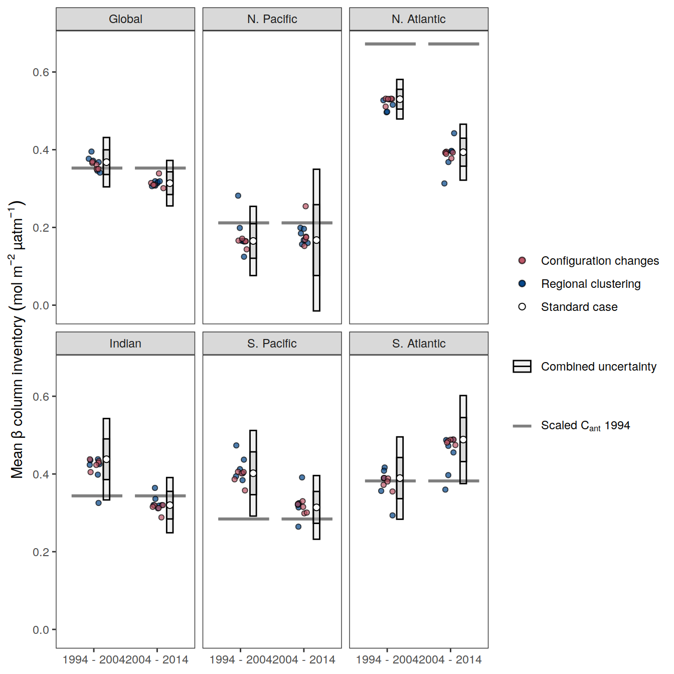
| Version | Author | Date |
|---|---|---|
| 2cca4eb | jens-daniel-mueller | 2023-01-10 |
| 0f2c9d5 | jens-daniel-mueller | 2022-12-08 |
| 3a7bab0 | jens-daniel-mueller | 2022-11-28 |
| 322b1c1 | jens-daniel-mueller | 2022-11-25 |
| 491f8b1 | jens-daniel-mueller | 2022-11-25 |
| 4da4d66 | jens-daniel-mueller | 2022-11-25 |
| 534ee74 | jens-daniel-mueller | 2022-11-25 |
| e924c80 | jens-daniel-mueller | 2022-11-17 |
| 8e1702d | jens-daniel-mueller | 2022-11-16 |
| ea34027 | jens-daniel-mueller | 2022-11-15 |
| 5520de8 | jens-daniel-mueller | 2022-11-15 |
| 1dad51a | jens-daniel-mueller | 2022-11-15 |
| ebc85e2 | jens-daniel-mueller | 2022-11-14 |
ggsave(path = here::here("output/publication"),
       filename = "FigS_beta_inventory.png",
       height = 6,
       width = 8,
       dpi = 600)
14.2.4 Biases
dcant_budget_basin_MLR_all_bias <-
  dcant_budget_basin_MLR_all_ensemble %>%
  filter(data_source %in% c("mod", "mod_truth")) %>%
  pivot_wider(names_from = data_source,
              values_from = dcant) %>%
  mutate(dcant_bias = mod - mod_truth,
         dcant_bias_rel = 100 * dcant_bias / mod_truth) %>%
  filter(period %in% two_decades)


dcant_budget_basin_MLR_all_bias <-
  dcant_budget_basin_MLR_all_bias %>%
  select(basin, period, MLR_basins, Version_ID_group, dcant = dcant_bias)

dcant_budget_basin_MLR_all_bias_uncertainty <-
  additive_uncertainty(dcant_budget_basin_MLR_all_bias)

delta_dcant_budget_basin_MLR_all_bias_uncertainty <-
  dcant_budget_basin_MLR_all_bias_uncertainty[[3]]
dcant_budget_basin_MLR_all_bias_uncertainty_contributions <-
  dcant_budget_basin_MLR_all_bias_uncertainty[[2]]
dcant_budget_basin_MLR_all_bias_uncertainty <-
  dcant_budget_basin_MLR_all_bias_uncertainty[[1]]


dcant_budget_basin_MLR_all_bias  %>%
  filter(period != "1994 - 2014",
         MLR_basins == unique(params_local_all$MLR_basins)) %>%
  ggplot(aes(period, dcant)) +
  geom_hline(yintercept = 0) +
  geom_jitter(
    data = dcant_budget_basin_MLR_all_bias %>%
      filter(period != "1994 - 2014",
             Version_ID_group == unique(params_local_all$Version_ID_group)),
    aes(fill = "Regional clustering",
        alpha = "Regional clustering"),
    shape = 21,
    position = position_jitter(width = 0.1, height = 0)
  ) +
  geom_point(
    aes(fill = "Configuration changes",
        alpha = "Configuration changes"),
    shape = 21,
    position = position_jitter(width = 0.1, height = 0)
  ) +
  geom_crossbar(
    data = dcant_budget_basin_MLR_all_bias_uncertainty,
    aes(
      x = period,
      y = std_case,
      ymin = std_case - sd*2,
      ymax = std_case + sd*2,
      linetype = "Combined uncertainty"
    ),
    width = 0.1,
    fill = "#BBBBBB",
    alpha = 0.2,
    position = position_nudge(x = 0.2)
  ) +
  geom_crossbar(
    data = dcant_budget_basin_MLR_all_bias_uncertainty,
    aes(
      x = period,
      y = std_case,
      ymin = std_case - sd,
      ymax = std_case + sd,
      alpha = "Combined uncertainty",
    ),
    width = 0.1,
    fill = "#BBBBBB",
    alpha = 0.4,
    position = position_nudge(x = 0.2)
  ) +
  geom_point(
    data = dcant_budget_basin_MLR_all_bias_uncertainty,
    aes(x = period,
        y = std_case,
        fill = "Standard case",
        alpha = "Standard case"),
    size = 2,
    shape = 21,
    position = position_nudge(x = 0.2)
  ) +
  scale_fill_manual(name = "group", values = c("#BB5566", "#004488", "white")) +
  scale_color_manual(values = c("grey50"), label = expression(Scaled~C[ant]~1994)) +
  scale_linetype(name = "X") +
  scale_alpha_manual(name = "group", values = c(0.7,0.7,1)) +
  scale_shape_manual(values = 95) +
  scale_y_continuous(name = dcant_bias_pgc_label) +
  guides(
    fill = guide_legend(order = 1),
    linetype = guide_legend(order = 2),
    alpha = guide_legend(order = 1)
  ) +
  facet_wrap(~ basin, ncol = 3, dir = "v", scales = "free_y") +
  theme(legend.title = element_blank(),
        axis.title.x = element_blank())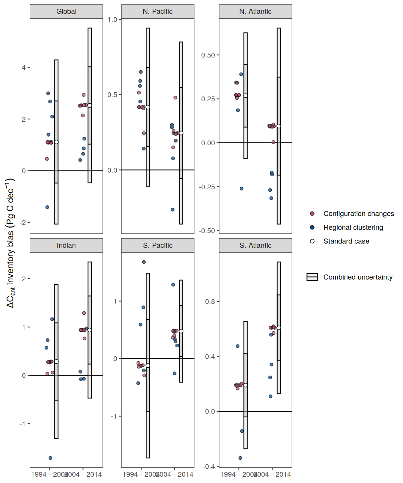
| Version | Author | Date |
|---|---|---|
| 0f2c9d5 | jens-daniel-mueller | 2022-12-08 |
| 3a7bab0 | jens-daniel-mueller | 2022-11-28 |
| 491f8b1 | jens-daniel-mueller | 2022-11-25 |
| 4da4d66 | jens-daniel-mueller | 2022-11-25 |
| 534ee74 | jens-daniel-mueller | 2022-11-25 |
| ea34027 | jens-daniel-mueller | 2022-11-15 |
| 5520de8 | jens-daniel-mueller | 2022-11-15 |
| 1dad51a | jens-daniel-mueller | 2022-11-15 |
| ebc85e2 | jens-daniel-mueller | 2022-11-14 |
| 6edad9b | jens-daniel-mueller | 2022-11-11 |
ggsave(path = here::here("output/publication"),
       filename = "FigS_dcant_bias_inventory_synthetic_data.png",
       height = 6,
       width = 8,
       dpi = 600)
14.3 Flow chart
dcant_budget_basin_MLR_all <-
  dcant_budget_basin_MLR_all %>%
  filter(basin != "Global")

dcant_budget_basin_MLR_all <- left_join(dcant_budget_basin_MLR_all,
                           co2_atm %>% rename(tref1 = year,
                                              pCO21 = pCO2))

dcant_budget_basin_MLR_all <- left_join(dcant_budget_basin_MLR_all,
                           co2_atm %>% rename(tref2 = year,
                                              pCO22 = pCO2))


dcant_budget_basin_MLR_all_plot <- dcant_budget_basin_MLR_all %>%
  filter(period != "1994 - 2014",
         data_source == "obs")
tcant_budget_basin_MLR <-
tcant_inv %>%
mutate(method = "layer",
data_source = "obs") %>%
group_by(basin) %>%
nest() %>%
mutate(budget = map(.x = data, ~m_dcant_budget(.x))) %>%
select(-data) %>%
unnest(budget)
tcant_budget_basin_MLR <-
full_join(tcant_budget_basin_MLR,
area_scaling %>% select(basin, scaling_factor)) %>%
mutate(value = value * scaling_factor) %>%
select(-scaling_factor)
tcant_budget_basin_MLR <- tcant_budget_basin_MLR %>%
mutate(pCO21 = 281,
tref1 = 1800,
tref2 = 1994)
tcant_budget_basin_MLR <- left_join(tcant_budget_basin_MLR,
co2_atm %>% rename(tref2 = year,
pCO22 = pCO2))
tcant_budget_basin_MLR <- tcant_budget_basin_MLR %>%
mutate(period = paste(tref1, tref2, sep = " - ")) %>%
filter(estimate == "dcant") %>%
select(-estimate) %>%
rename(dcant = value)
dcant_budget_basin_MLR_all_plot <- bind_rows(
dcant_budget_basin_MLR_all_plot,
tcant_budget_basin_MLR)
dcant_budget_basin_MLR_all_plot <-
left_join(dcant_budget_basin_MLR_all_plot,
dcant_budget_basin_MLR_all_ensemble_summary)14.3.1 Absolute
g1 <- dcant_budget_basin_MLR_all_plot %>%
  filter(period != "1800 - 1994") %>%
  ggplot(aes(
    y = dcant,
    x = period,
    alluvium = basin,
    fill  = basin,
    stratum = basin
  )) +
  stat_alluvium(decreasing = FALSE) +
  stat_stratum(decreasing = FALSE) +
  stat_stratum(geom = "text",
               decreasing = FALSE,
               aes(label = paste(
                 round(after_stat(max-min),1)
                 # 100*round(after_stat(prop), 2), "%"
                 ))) +
  ggrepel::geom_label_repel(
    data = dcant_budget_basin_MLR_all_plot %>% filter(period == "2004 - 2014"),
    stat = "stratum",
    size = 4,
    nudge_x = .5,
    point.padding = 3,
    aes(fill = basin, label = basin),
    decreasing = FALSE
  )+
  scale_fill_brewer(palette = "Paired", guide = "none") +
  scale_y_continuous(limits = c(0, 32), expand = c(0, 0)) +
  labs(y = dcant_pgc_label) +
  theme(axis.text.x = element_text(angle = 45, hjust = 1),
        axis.title.x = element_blank()) +
  theme_classic()


newdat <- tibble(layer_data(g1))

change <-
  newdat %>%
  select(x, alluvium, count) %>%
  pivot_wider(names_from = x,
              values_from = count) %>%
  mutate(dcant_change = round(100*(`2` - `1`) / `1`)) %>%
  select(alluvium, dcant_change)

coord <- newdat %>%
  filter(x == 2) %>%
  select(x, y, alluvium)

new_layer <- full_join(
  change,
  coord
)

new_layer <- new_layer %>%
  mutate(dcant_change = as.character(dcant_change),
         dcant_change = if_else(str_detect(dcant_change, "-"),
                                dcant_change,
                                paste0("+", dcant_change)),
         dcant_change = paste(dcant_change, "%"))

g1 +
  geom_text(data = new_layer,
            aes(
              x = x - 0.3,
              y = y,
              label = dcant_change
            ),
            inherit.aes = FALSE)
g2 <- dcant_budget_basin_MLR_all_plot %>%
filter(period != "1800 - 1994") %>%
ggplot(aes(
y = dcant,
x = period,
alluvium = basin,
fill = basin,
stratum = basin,
label = basin
)) +
geom_alluvium() +
geom_stratum() +
stat_stratum(geom = "text",
aes(label = paste(
round(after_stat(count),1)
# 100*round(after_stat(prop), 2), "%"
))) +
ggrepel::geom_label_repel(
data = dcant_budget_basin_MLR_all_plot %>% filter(period == "2004 - 2014"),
stat = "stratum",
size = 4,
nudge_x = .5,
point.padding = 3,
aes(fill = basin)
)+
scale_fill_brewer(palette = "Paired", guide = "none") +
scale_color_brewer(palette = "Paired", guide = "none") +
scale_y_continuous(limits = c(0, 33), expand = c(0, 0)) +
guides(y = "none") +
labs(title = dcant_pgc_label) +
theme_classic() +
theme(axis.text.x = element_text(angle = 45, hjust = 1),
axis.title.x = element_blank(),
axis.title.y = element_blank(),
plot.title = element_text(hjust = 0.5))
newdat <- tibble(layer_data(g2))
change_basin <-
newdat %>%
select(x, alluvium, count) %>%
pivot_wider(names_from = x,
values_from = count) %>%
mutate(dcant_change = round(100*(`2` - `1`) / `1`)) %>%
select(alluvium, dcant_change)
coord_basin <- newdat %>%
filter(x == 2) %>%
select(x, y, alluvium)
new_layer_basin <- full_join(
change_basin,
coord_basin
)
new_layer_basin <- new_layer_basin %>%
mutate(dcant_change = as.character(dcant_change),
dcant_change = if_else(str_detect(dcant_change, "-"),
dcant_change,
paste0("+", dcant_change)),
dcant_change = paste(dcant_change, "%"))
new_layer_total <-
newdat %>%
select(x, alluvium, count) %>%
group_by(x) %>%
summarise(dcant_change = sum(count)) %>%
ungroup()
new_layer_total <- new_layer_total %>%
mutate(y = dcant_change,
dcant_change = as.character(round(dcant_change,1)),
dcant_change = paste("global:",dcant_change))
g2 +
geom_text(data = new_layer_basin,
aes(
x = x - 0.3,
y = y,
label = dcant_change
),
inherit.aes = FALSE) +
geom_label(data = new_layer_total,
aes(
x = x,
y = y + 1,
label = dcant_change
),
inherit.aes = FALSE)14.3.2 Scaled
dcant_budget_basin_MLR_all_plot <- left_join(dcant_budget_basin_MLR_all_plot,
                           co2_atm %>% rename(tref1 = year,
                                              pCO21 = pCO2))

dcant_budget_basin_MLR_all_plot <- left_join(dcant_budget_basin_MLR_all_plot,
                           co2_atm %>% rename(tref2 = year,
                                              pCO22 = pCO2))

dcant_budget_basin_MLR_all_plot <- dcant_budget_basin_MLR_all_plot %>%
  mutate(delta_pCO2 = pCO22 - pCO21,
         beta = dcant / delta_pCO2,
         dcant_sd_scaled = dcant_sd / delta_pCO2) %>%
  select(-starts_with("pCO2"))


dcant_budget_global_all_ensemble_summary <- left_join(dcant_budget_global_all_ensemble_summary,
                           co2_atm %>% rename(tref1 = year,
                                              pCO21 = pCO2))

dcant_budget_global_all_ensemble_summary <- left_join(dcant_budget_global_all_ensemble_summary,
                           co2_atm %>% rename(tref2 = year,
                                              pCO22 = pCO2))

dcant_budget_global_all_ensemble_summary <- dcant_budget_global_all_ensemble_summary %>%
  mutate(delta_pCO2 = pCO22 - pCO21,
         beta = dcant_mean / delta_pCO2,
         dcant_sd_scaled = dcant_sd / delta_pCO2) %>%
  select(-starts_with("pCO2"))
g2 <- dcant_budget_basin_MLR_all_plot %>%
filter(period != "1800 - 1994") %>%
ggplot(aes(
y = beta,
x = period,
alluvium = basin,
fill = basin,
stratum = basin,
label = basin
)) +
geom_alluvium() +
geom_stratum() +
stat_stratum(geom = "text",
aes(label = paste(
round(after_stat(count),2)
# 100*round(after_stat(prop), 2), "%"
))) +
ggrepel::geom_label_repel(
data = dcant_budget_basin_MLR_all_plot %>% filter(period == "2004 - 2014"),
stat = "stratum",
size = 4,
nudge_x = .5,
point.padding = 3,
aes(fill = basin)
)+
scale_fill_brewer(palette = "Paired", guide = "none") +
scale_color_brewer(palette = "Paired", guide = "none") +
# scale_y_continuous(limits = c(0, 33), expand = c(0, 0)) +
guides(y = "none") +
labs(title = beta_inv_label) +
theme_classic() +
theme(axis.text.x = element_text(angle = 45, hjust = 1),
axis.title.x = element_blank(),
axis.title.y = element_blank(),
plot.title = element_text(hjust = 0.5))
newdat <- tibble(layer_data(g2))
change_basin <-
newdat %>%
select(x, alluvium, count) %>%
pivot_wider(names_from = x,
values_from = count) %>%
mutate(dcant_change = round(100*(`2` - `1`) / `1`)) %>%
select(alluvium, dcant_change)
coord_basin <- newdat %>%
filter(x == 2) %>%
select(x, y, alluvium)
new_layer_basin <- full_join(
change_basin,
coord_basin
)
new_layer_basin <- new_layer_basin %>%
mutate(dcant_change = as.character(dcant_change),
dcant_change = if_else(str_detect(dcant_change, "-"),
dcant_change,
paste0("+", dcant_change)),
dcant_change = paste(dcant_change, "%"))
new_layer_total <-
newdat %>%
select(x, alluvium, count) %>%
group_by(x) %>%
summarise(dcant_change = sum(count)) %>%
ungroup()
new_layer_total <- new_layer_total %>%
mutate(y = dcant_change,
dcant_change = as.character(round(dcant_change,2)),
dcant_change = paste("global:",dcant_change))
g2 +
geom_text(data = new_layer_basin,
aes(
x = x - 0.3,
y = y,
label = dcant_change
),
inherit.aes = FALSE) +
geom_label(data = new_layer_total,
aes(
x = x,
y = y + 0.05,
label = dcant_change
),
inherit.aes = FALSE)g2 <- dcant_budget_basin_MLR_all_plot %>%
ggplot(aes(
y = beta,
x = period,
alluvium = basin,
fill = basin,
stratum = basin,
label = basin
)) +
geom_alluvium() +
geom_stratum() +
stat_stratum(geom = "text",
aes(label = paste(
round(after_stat(count),2)
# 100*round(after_stat(prop), 2), "%"
))) +
ggrepel::geom_label_repel(
data = dcant_budget_basin_MLR_all_plot %>% filter(period == "2004 - 2014"),
stat = "stratum",
size = 4,
nudge_x = .5,
point.padding = 3,
aes(fill = basin)
)+
scale_fill_brewer(palette = "Paired", guide = "none") +
scale_color_brewer(palette = "Paired", guide = "none") +
scale_y_continuous(limits = c(0, 1.7), expand = c(0, 0)) +
guides(y = "none") +
labs(title = beta_inv_label) +
theme_classic() +
theme(axis.text.x = element_text(angle = 45, hjust = 1),
axis.title.x = element_blank(),
axis.title.y = element_blank(),
plot.title = element_text(hjust = 0.5))
newdat <- tibble(layer_data(g2))
change_basin <-
newdat %>%
select(x, alluvium, count) %>%
group_by(alluvium) %>%
arrange(x) %>%
mutate(dcant_change = round(100*(count - lag(count)) / lag(count))) %>%
ungroup()
coord_basin <- newdat %>%
select(x, y, alluvium)
new_layer_basin <- left_join(
change_basin %>% drop_na(),
coord_basin
)
new_layer_basin <- new_layer_basin %>%
mutate(dcant_change = as.character(dcant_change),
dcant_change = if_else(str_detect(dcant_change, "-"),
dcant_change,
paste0("+", dcant_change)),
dcant_change = paste(dcant_change, "%"))
new_layer_total <-
newdat %>%
select(x, alluvium, count) %>%
group_by(x) %>%
summarise(dcant_change = sum(count)) %>%
ungroup()
new_layer_total <- new_layer_total %>%
mutate(y = dcant_change,
dcant_change = as.character(round(dcant_change,2)),
dcant_change = paste("global:",dcant_change))
g2 +
geom_text(data = new_layer_basin,
aes(
x = x - 0.3,
y = y,
label = dcant_change
),
inherit.aes = FALSE) +
geom_label(data = new_layer_total,
aes(
x = x,
y = y + 0.1,
label = dcant_change
),
inherit.aes = FALSE)g2 <- dcant_budget_basin_MLR_all_plot %>%
ggplot(aes(
y = beta,
x = period,
alluvium = basin,
fill = basin,
stratum = basin,
label = basin
)) +
geom_alluvium() +
geom_stratum() +
ggrepel::geom_label_repel(
data = dcant_budget_basin_MLR_all_plot %>% filter(period == "2004 - 2014"),
stat = "stratum",
size = 4,
nudge_x = .5,
point.padding = 3,
aes(fill = basin)
)+
scale_fill_brewer(palette = "Paired", guide = "none") +
scale_color_brewer(palette = "Paired", guide = "none") +
scale_y_continuous(limits = c(0, 1.6), expand = c(0, 0)) +
guides(y = "none") +
labs(title = beta_inv_label) +
theme_classic() +
theme(axis.text.x = element_text(angle = 45, hjust = 1),
axis.title.x = element_blank(),
axis.title.y = element_blank(),
plot.title = element_text(hjust = 0.5))
newdat <- tibble(layer_data(g2))
# construct budget labels
budget_basin <-
newdat %>%
select(x, y, alluvium, count)
budget_layer_basin <- budget_basin %>%
mutate(dcant = as.character(round(count,2)))
# construct uncertainty labels
uncertainty_basin <-
dcant_budget_basin_MLR_all_plot %>%
mutate(x = fct_recode(period,
"2" = "1994 - 2004",
"3" = "2004 - 2014")) %>%
select(x, alluvium = basin, dcant_sd_scaled) %>%
drop_na() %>%
arrange(x, alluvium)
coord_basin <- newdat %>%
select(x, y, alluvium) %>%
filter(x != 1)
uncertainty_layer_basin <- bind_cols(
coord_basin,
uncertainty_basin %>% select(dcant_sd_scaled),
)
# construct change labels
change_basin <-
newdat %>%
select(x, alluvium, count) %>%
group_by(alluvium) %>%
arrange(x) %>%
mutate(dcant_change_abs = count - lag(count),
dcant_change = round(100*(dcant_change_abs) / lag(count))) %>%
ungroup()
coord_basin <- newdat %>%
select(x, y, alluvium)
new_layer_basin <- left_join(
change_basin %>% drop_na(),
coord_basin
)
new_layer_basin <- new_layer_basin %>%
mutate(dcant_change = as.character(dcant_change),
dcant_change = if_else(str_detect(dcant_change, "-"),
dcant_change,
paste0("+", dcant_change)),
dcant_change = paste0(dcant_change, "%"))
# construct global budget labels
new_layer_total <-
newdat %>%
select(x, alluvium, count) %>%
group_by(x) %>%
summarise(dcant_change = sum(count)) %>%
ungroup()
dcant_sd_scaled <- round(c(
0.24,
dcant_budget_global_all_ensemble_summary %>%
pull(dcant_sd_scaled)
), 2)
new_layer_total <- bind_cols(new_layer_total, dcant_sd_scaled = dcant_sd_scaled)
new_layer_total <- new_layer_total %>%
mutate(y = dcant_change,
dcant_sd_scaled_rel = round(100 * dcant_sd_scaled/dcant_change),
dcant_change = as.character(round(dcant_change,2)),
dcant_sd_scaled = round(dcant_sd_scaled,1),
dcant_change = paste0(dcant_change, "\n(±", dcant_sd_scaled, ")"))
# basin change + uncertainty
budget_layer_basin <- full_join(budget_layer_basin,
uncertainty_layer_basin)
budget_layer_basin <-
budget_layer_basin %>%
mutate(dcant_sd_scaled_rel = 100*dcant_sd_scaled/count,
dcant_sd_scaled_rel = as.character(round(dcant_sd_scaled_rel)),
dcant_sd_scaled_numeric = dcant_sd_scaled,
dcant_sd_scaled = round(dcant_sd_scaled, 2),
dcant_sd_scaled = paste0("(±", dcant_sd_scaled, ")"),
dcant_label = if_else(dcant_sd_scaled != "(±NA)",
paste0(dcant, "\n", dcant_sd_scaled),
dcant))
# uncertainty changes
uncertainty_changes <- budget_layer_basin %>%
select(x, alluvium, dcant_sd_scaled = dcant_sd_scaled_numeric) %>%
group_by(alluvium) %>%
mutate(dcant_change_uncert = sqrt(dcant_sd_scaled^2 + lag(dcant_sd_scaled)^2)) %>%
ungroup()
new_layer_basin <- left_join(new_layer_basin, uncertainty_changes) %>%
mutate(dcant_change_uncert_rel = 100*dcant_change_uncert/abs((count + lag(count))/2),
dcant_change_label = if_else(!is.na(dcant_change_uncert),
paste0(dcant_change, "\n(±", round(dcant_change_uncert_rel), "%)"),
dcant_change))
g2 +
geom_text(data = budget_layer_basin,
aes(
x = x,
y = y,
label = dcant_label
),
size = 3,
inherit.aes = FALSE) +
geom_text(data = new_layer_basin,
aes(
x = x - 0.3,
y = y,
label = dcant_change_label
),
size = 4,
inherit.aes = FALSE)
# geom_label(data = new_layer_total,
# aes(
# x = x,
# y = y + 0.13,
# label = dcant_change
# ),
# size = 4,
# inherit.aes = FALSE)
# ggsave(path = here::here("output/publication"),
# filename = "Fig_budget_beta_basin_hemisphere.png",
# height = 6,
# width = 8)14.4 Depth layer
dcant_budget_change <- dcant_budget_basin_MLR_layer_all %>%
  filter(estimate == "dcant",
         period != "1994 - 2014",
         inv_depth <= 3000,
         data_source == "obs") %>%
  rename(dcant = value) %>%
  select(-c(tref1, tref2, Version_ID)) %>%
  pivot_wider(names_from = period,
              values_from = dcant) %>%
  mutate(sign = if_else(`2004 - 2014` - `1994 - 2004` > 0,
                        "increase",
                        "decrease"))

dcant_budget_layer <- dcant_budget_basin_MLR_layer_all %>%
  filter(estimate == "dcant",
         period != "1994 - 2014",
         inv_depth <= 3400,
         data_source == "obs") %>%
  rename(dcant = value) %>%
  group_by(basin, period, data_source) %>%
  mutate(dcant = if_else(is.na(lead(dcant)), 888, dcant),
         dcant = na_if(dcant, 888)) %>%
  fill(dcant) %>%
  ungroup()

dcant_budget_layer %>%
  ggplot() +
  geom_hline(yintercept = 0) +
  geom_rect(
    data = dcant_budget_change,
    aes(
      xmin = inv_depth - 250,
      xmax = inv_depth + 250,
      ymin = `1994 - 2004`,
      ymax = `2004 - 2014`,
      fill = sign
    ),
    alpha = 0.4
  ) +
  geom_step(aes(inv_depth - 250, dcant, col = period), direction = "vh",
            size = 1) +
  coord_flip() +
  scale_x_reverse(breaks = seq(0, 3000, 500)) +
  scale_color_brewer(palette = "Set1", direction = -1, name = "period") +
  scale_fill_brewer(palette = "Set1", direction = -1, name = "") +
  facet_wrap(~ basin, ncol = 3, dir = "v") +
  labs(y = dcant_layer_budget_label,
       x = "Depth (m)") +
      theme(legend.position = c(0.8,0.2))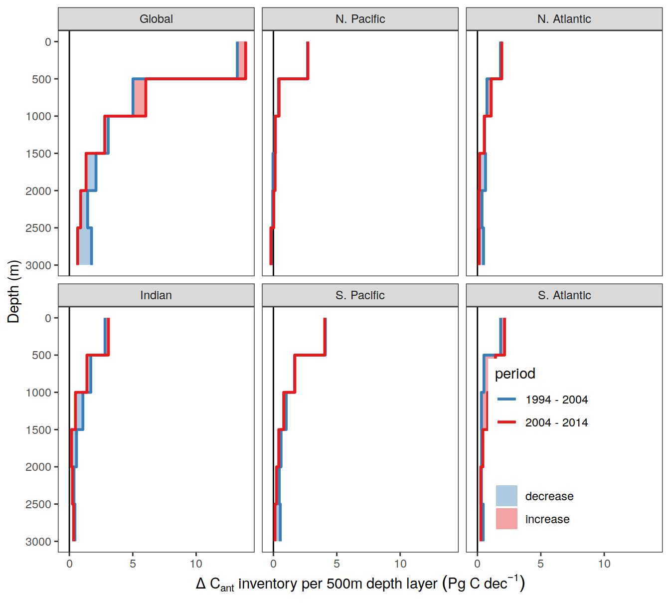
| Version | Author | Date |
|---|---|---|
| 0f2c9d5 | jens-daniel-mueller | 2022-12-08 |
| 3a7bab0 | jens-daniel-mueller | 2022-11-28 |
| ea34027 | jens-daniel-mueller | 2022-11-15 |
| 5520de8 | jens-daniel-mueller | 2022-11-15 |
| ebc85e2 | jens-daniel-mueller | 2022-11-14 |
| 2345935 | jens-daniel-mueller | 2022-10-29 |
| 91052ae | jens-daniel-mueller | 2022-10-20 |
| 78dbb27 | jens-daniel-mueller | 2022-08-11 |
| 302d289 | jens-daniel-mueller | 2022-08-11 |
| fea41c1 | jens-daniel-mueller | 2022-07-20 |
| d2ae54c | jens-daniel-mueller | 2022-07-18 |
| 2695085 | jens-daniel-mueller | 2022-07-17 |
| 26e9496 | jens-daniel-mueller | 2022-07-12 |
dcant_budget_basin_MLR_layer_all_uncertainty <-
dcant_budget_basin_MLR_layer_all_ensemble %>%
filter(estimate == "dcant",
period != "1994 - 2014",
inv_depth <= 3400) %>%
rename(dcant = value) %>%
select(-c(method, estimate, Version_ID, tref1, tref2)) %>%
group_by(basin, period, data_source, MLR_basins, Version_ID_group) %>%
mutate(dcant = if_else(is.na(lead(dcant)), 888, dcant),
dcant = na_if(dcant, 888)) %>%
fill(dcant) %>%
ungroup()
dcant_budget_basin_MLR_layer_all_uncertainty <- additive_uncertainty(dcant_budget_basin_MLR_layer_all_uncertainty)
delta_dcant_budget_basin_MLR_layer_all_uncertainty <- dcant_budget_basin_MLR_layer_all_uncertainty[[3]]
dcant_budget_basin_MLR_layer_all_uncertainty_contributions <- dcant_budget_basin_MLR_layer_all_uncertainty[[2]]
dcant_budget_basin_MLR_layer_all_uncertainty <- dcant_budget_basin_MLR_layer_all_uncertainty[[1]]
p_dcant_budget_depth_layer <-
dcant_budget_basin_MLR_layer_all_uncertainty %>%
filter(data_source == "obs") %>%
ggplot() +
geom_hline(yintercept = 0, size = 0.1) +
geom_rect(
aes(
xmin = inv_depth - 250,
xmax = inv_depth + 250,
ymin = std_case - sd*2,
ymax = std_case + sd*2,
fill = period
),
alpha = 0.2
) +
geom_rect(
aes(
xmin = inv_depth - 250,
xmax = inv_depth + 250,
ymin = std_case - sd,
ymax = std_case + sd,
fill = period
),
alpha = 0.4
) +
geom_step(aes(inv_depth - 250, std_case, col = period), direction = "vh",
size = 1) +
coord_flip() +
scale_x_reverse(breaks = seq(0, 3000, 500), limits = c(3000, 0), expand = c(0,0)) +
scale_color_manual(values = c("#EE7733", "#009988"), name = "Mean \u00B1 1σ/2σ") +
scale_fill_manual(values = c("#EE7733", "#009988"), name = "Mean \u00B1 1σ/2σ") +
labs(y = dcant_layer_budget_label,
x = "Depth (m)") +
facet_wrap(~ basin, ncol = 3, dir = "v", scales = "free_x") +
theme(legend.position = c(0.9, 0.1))
p_dcant_budget_depth_layer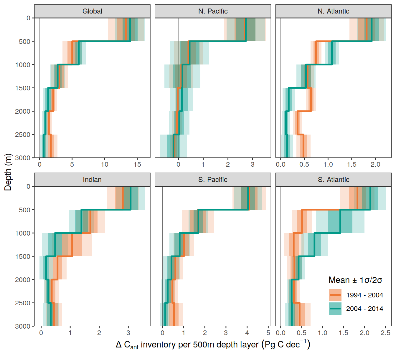
| Version | Author | Date |
|---|---|---|
| 3a7bab0 | jens-daniel-mueller | 2022-11-28 |
| 322b1c1 | jens-daniel-mueller | 2022-11-25 |
| 491f8b1 | jens-daniel-mueller | 2022-11-25 |
| 4da4d66 | jens-daniel-mueller | 2022-11-25 |
| 534ee74 | jens-daniel-mueller | 2022-11-25 |
| ea34027 | jens-daniel-mueller | 2022-11-15 |
| 5520de8 | jens-daniel-mueller | 2022-11-15 |
| 1dad51a | jens-daniel-mueller | 2022-11-15 |
| ebc85e2 | jens-daniel-mueller | 2022-11-14 |
| 6edad9b | jens-daniel-mueller | 2022-11-11 |
| 16beb51 | jens-daniel-mueller | 2022-11-08 |
| b92657d | jens-daniel-mueller | 2022-11-08 |
| 7275091 | jens-daniel-mueller | 2022-11-05 |
| 99610ed | jens-daniel-mueller | 2022-11-01 |
| 7060801 | jens-daniel-mueller | 2022-10-31 |
| ecb84c1 | jens-daniel-mueller | 2022-10-30 |
| 2345935 | jens-daniel-mueller | 2022-10-29 |
| 91052ae | jens-daniel-mueller | 2022-10-20 |
| 78dbb27 | jens-daniel-mueller | 2022-08-11 |
| 302d289 | jens-daniel-mueller | 2022-08-11 |
| fea41c1 | jens-daniel-mueller | 2022-07-20 |
| d803308 | jens-daniel-mueller | 2022-07-19 |
| b1f7ab3 | jens-daniel-mueller | 2022-07-18 |
| d2ae54c | jens-daniel-mueller | 2022-07-18 |
| 2695085 | jens-daniel-mueller | 2022-07-17 |
| 535196a | jens-daniel-mueller | 2022-07-17 |
| afb27ad | jens-daniel-mueller | 2022-07-15 |
| b492b46 | jens-daniel-mueller | 2022-07-15 |
| bd24a0f | jens-daniel-mueller | 2022-07-15 |
| 17cd1d1 | jens-daniel-mueller | 2022-07-13 |
| 26e9496 | jens-daniel-mueller | 2022-07-12 |
p_dcant_profiles + p_dcant_budget_depth_layer +
plot_layout(ncol = 1) +
plot_annotation(tag_levels = 'A')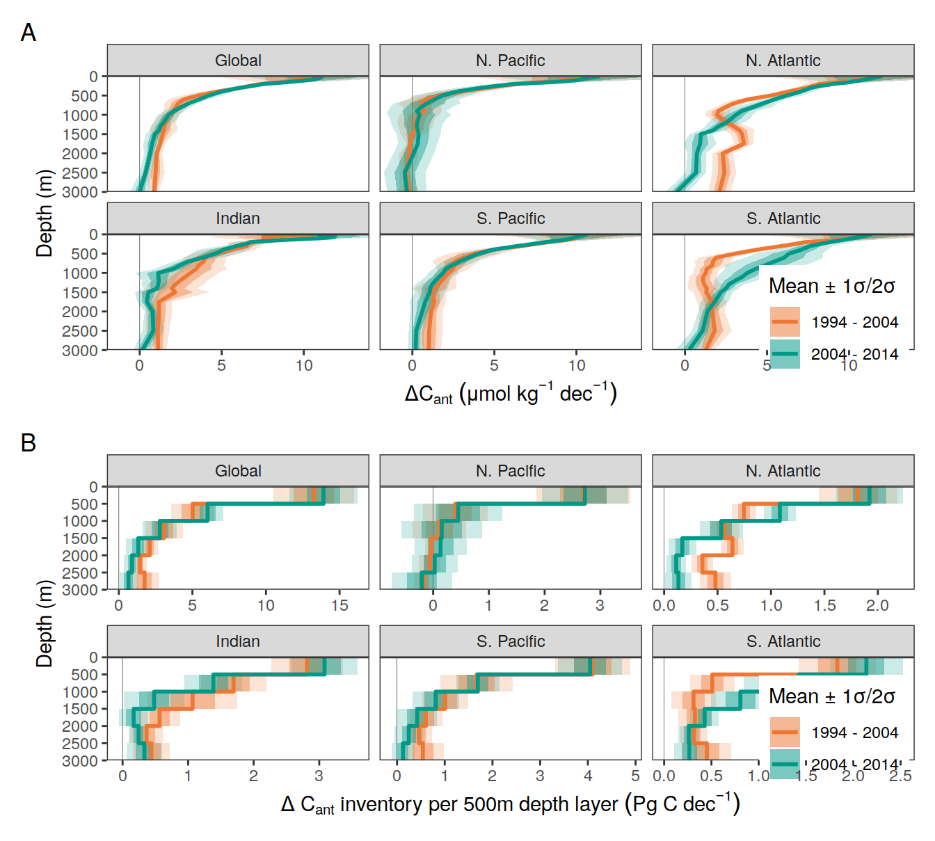
| Version | Author | Date |
|---|---|---|
| 3a7bab0 | jens-daniel-mueller | 2022-11-28 |
| 322b1c1 | jens-daniel-mueller | 2022-11-25 |
| 491f8b1 | jens-daniel-mueller | 2022-11-25 |
| 4da4d66 | jens-daniel-mueller | 2022-11-25 |
| 534ee74 | jens-daniel-mueller | 2022-11-25 |
| ea34027 | jens-daniel-mueller | 2022-11-15 |
| 5520de8 | jens-daniel-mueller | 2022-11-15 |
| 1dad51a | jens-daniel-mueller | 2022-11-15 |
| ebc85e2 | jens-daniel-mueller | 2022-11-14 |
| 6edad9b | jens-daniel-mueller | 2022-11-11 |
| 16beb51 | jens-daniel-mueller | 2022-11-08 |
| b92657d | jens-daniel-mueller | 2022-11-08 |
| 7275091 | jens-daniel-mueller | 2022-11-05 |
| 99610ed | jens-daniel-mueller | 2022-11-01 |
| 7060801 | jens-daniel-mueller | 2022-10-31 |
| ecb84c1 | jens-daniel-mueller | 2022-10-30 |
| 2345935 | jens-daniel-mueller | 2022-10-29 |
| 91052ae | jens-daniel-mueller | 2022-10-20 |
| 051b911 | jens-daniel-mueller | 2022-09-07 |
| 75bd58c | jens-daniel-mueller | 2022-09-07 |
| 1c6de0d | jens-daniel-mueller | 2022-09-07 |
| 78dbb27 | jens-daniel-mueller | 2022-08-11 |
| 302d289 | jens-daniel-mueller | 2022-08-11 |
| fea41c1 | jens-daniel-mueller | 2022-07-20 |
| d803308 | jens-daniel-mueller | 2022-07-19 |
ggsave(path = here::here("output/publication"),
filename = "Fig_dcant_profiles_and_depth_layer_inventories.png",
height = 12,
width = 8,
dpi = 600)p_dcant_budget_depth_layer_mod <-
dcant_budget_basin_MLR_layer_all_uncertainty %>%
filter(data_source != "obs") %>%
mutate(data_source = case_when(
data_source == "mod" ~ "Reconstruction",
data_source == "mod_truth" ~ "Model truth"
)) %>%
ggplot() +
geom_hline(yintercept = 0, size = 0.1) +
geom_rect(
aes(
xmin = inv_depth - 250,
xmax = inv_depth + 250,
ymin = std_case - sd,
ymax = std_case + sd,
fill = data_source
),
alpha = 0.2
) +
geom_rect(
aes(
xmin = inv_depth - 250,
xmax = inv_depth + 250,
ymin = std_case - sd*2,
ymax = std_case + sd*2,
fill = data_source
),
alpha = 0.4
) +
geom_step(aes(inv_depth - 250, std_case, col = data_source), direction = "vh",
size = 1) +
coord_flip() +
scale_x_reverse(breaks = seq(0, 3000, 500), limits = c(3000, 0), expand = c(0,0)) +
scale_color_manual(values = c("#009988", "#EE7733"), name = "Mean \u00B1 2σ") +
scale_fill_manual(values = c("#009988", "#EE7733"), name = "Mean \u00B1 2σ") +
labs(y = dcant_layer_budget_label,
x = "Depth (m)") +
facet_grid(period ~ basin, scales = "free_x") +
theme(legend.position = "none")
p_dcant_budget_depth_layer_mod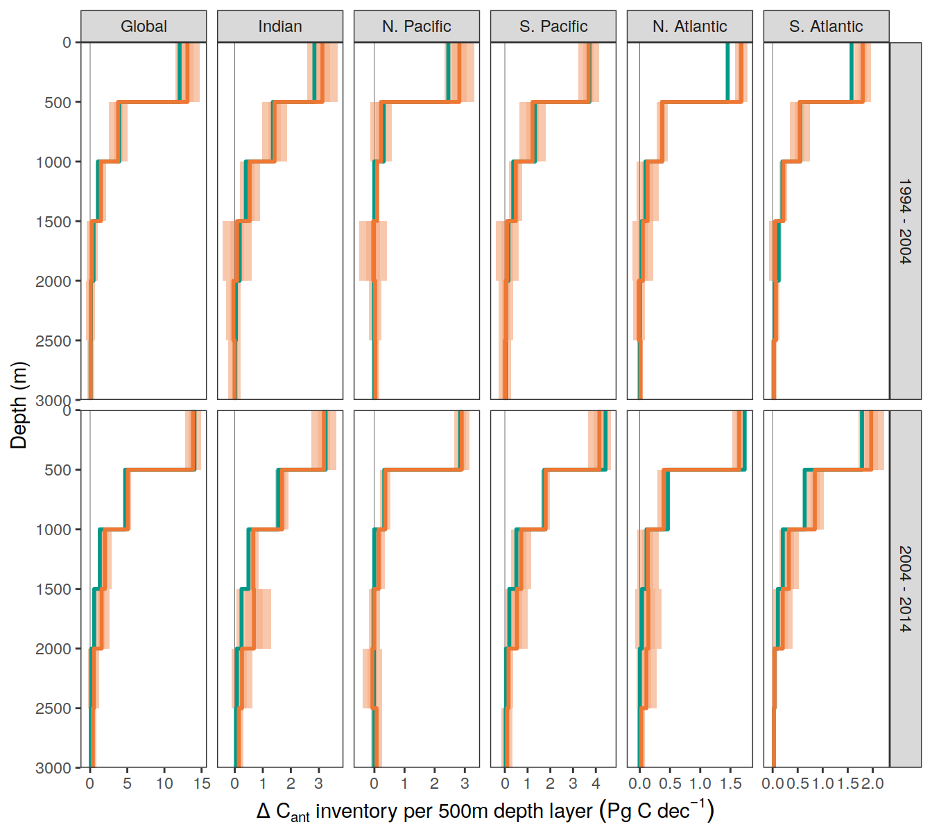
| Version | Author | Date |
|---|---|---|
| 3a7bab0 | jens-daniel-mueller | 2022-11-28 |
| 322b1c1 | jens-daniel-mueller | 2022-11-25 |
| 491f8b1 | jens-daniel-mueller | 2022-11-25 |
| 4da4d66 | jens-daniel-mueller | 2022-11-25 |
| 534ee74 | jens-daniel-mueller | 2022-11-25 |
| ea34027 | jens-daniel-mueller | 2022-11-15 |
| 5520de8 | jens-daniel-mueller | 2022-11-15 |
| 1dad51a | jens-daniel-mueller | 2022-11-15 |
| ebc85e2 | jens-daniel-mueller | 2022-11-14 |
| 6edad9b | jens-daniel-mueller | 2022-11-11 |
| 16beb51 | jens-daniel-mueller | 2022-11-08 |
| b92657d | jens-daniel-mueller | 2022-11-08 |
| 7275091 | jens-daniel-mueller | 2022-11-05 |
| 99610ed | jens-daniel-mueller | 2022-11-01 |
| 7060801 | jens-daniel-mueller | 2022-10-31 |
| ecb84c1 | jens-daniel-mueller | 2022-10-30 |
| 2345935 | jens-daniel-mueller | 2022-10-29 |
| 91052ae | jens-daniel-mueller | 2022-10-20 |
| 78dbb27 | jens-daniel-mueller | 2022-08-11 |
| 302d289 | jens-daniel-mueller | 2022-08-11 |
| 318fefe | jens-daniel-mueller | 2022-08-11 |
p_dcant_profiles_mod + p_dcant_budget_depth_layer_mod +
plot_layout(ncol = 1) +
plot_annotation(tag_levels = 'A')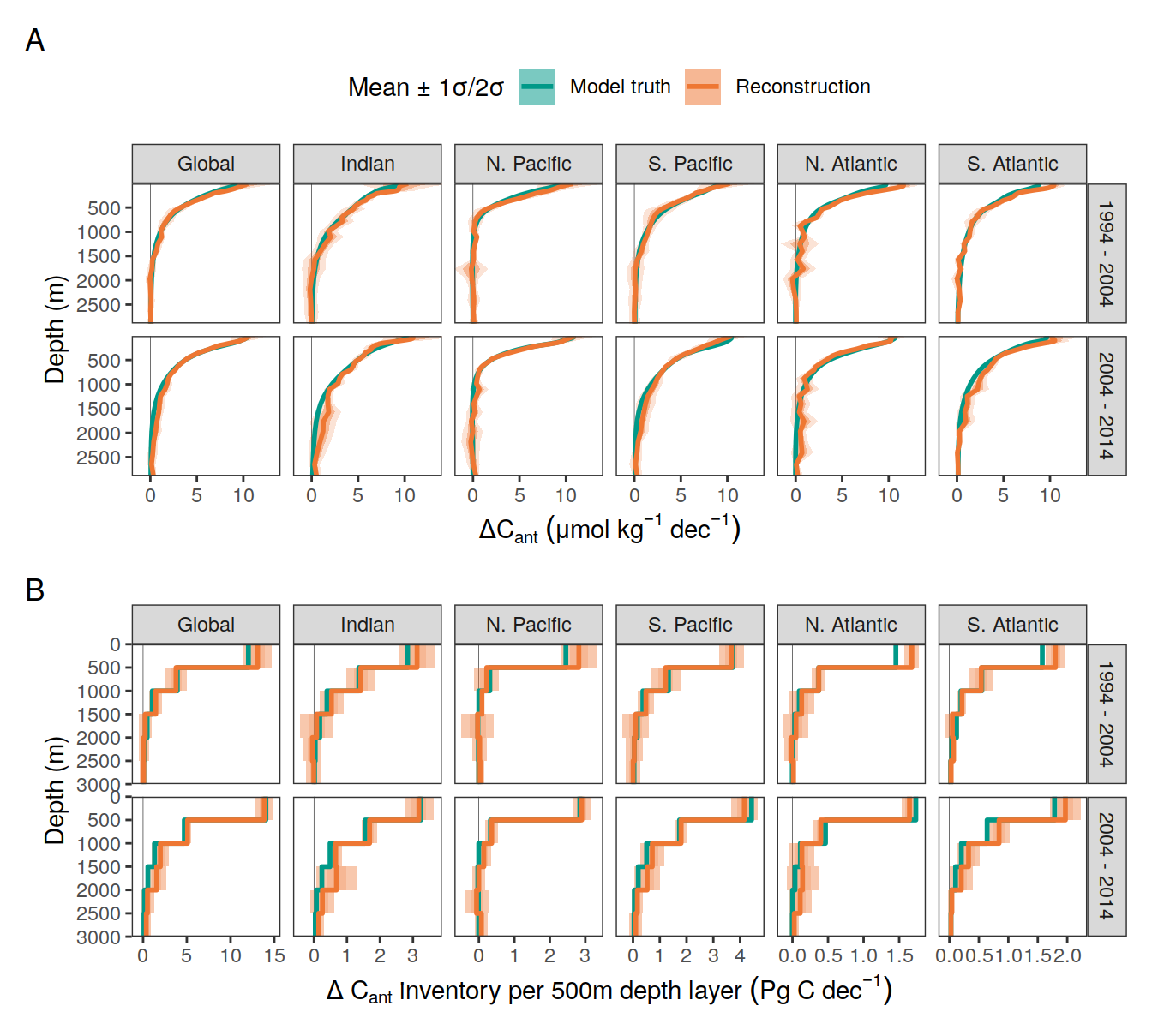
| Version | Author | Date |
|---|---|---|
| 3a7bab0 | jens-daniel-mueller | 2022-11-28 |
| 322b1c1 | jens-daniel-mueller | 2022-11-25 |
| 491f8b1 | jens-daniel-mueller | 2022-11-25 |
| 4da4d66 | jens-daniel-mueller | 2022-11-25 |
| 534ee74 | jens-daniel-mueller | 2022-11-25 |
| ea34027 | jens-daniel-mueller | 2022-11-15 |
| 5520de8 | jens-daniel-mueller | 2022-11-15 |
| 1dad51a | jens-daniel-mueller | 2022-11-15 |
| ebc85e2 | jens-daniel-mueller | 2022-11-14 |
| 6edad9b | jens-daniel-mueller | 2022-11-11 |
| 16beb51 | jens-daniel-mueller | 2022-11-08 |
| b92657d | jens-daniel-mueller | 2022-11-08 |
| 7275091 | jens-daniel-mueller | 2022-11-05 |
| 99610ed | jens-daniel-mueller | 2022-11-01 |
| 7060801 | jens-daniel-mueller | 2022-10-31 |
| ecb84c1 | jens-daniel-mueller | 2022-10-30 |
| 2345935 | jens-daniel-mueller | 2022-10-29 |
| 91052ae | jens-daniel-mueller | 2022-10-20 |
| 051b911 | jens-daniel-mueller | 2022-09-07 |
| 75bd58c | jens-daniel-mueller | 2022-09-07 |
| 1c6de0d | jens-daniel-mueller | 2022-09-07 |
| 78dbb27 | jens-daniel-mueller | 2022-08-11 |
| 302d289 | jens-daniel-mueller | 2022-08-11 |
| 318fefe | jens-daniel-mueller | 2022-08-11 |
ggsave(path = here::here("output/publication"),
filename = "FigS_dcant_profiles_and_depth_layer_inventories_synthetic_data.png",
height = 10,
width = 7,
dpi = 600)dcant_budget_change <- dcant_budget_basin_MLR_layer_all %>%
filter(estimate == "dcant",
period != "1994 - 2014",
inv_depth <= 3000,
data_source == "obs") %>%
rename(dcant = value) %>%
arrange(inv_depth) %>%
group_by(data_source, basin, period) %>%
mutate(dcant_cum = cumsum(dcant)) %>%
ungroup() %>%
select(-c(tref2, Version_ID, dcant)) %>%
pivot_wider(names_from = period,
values_from = dcant_cum) %>%
mutate(sign = if_else(`2004 - 2014` - `1994 - 2004` > 0,
"increase",
"decrease"))
dcant_budget_layer <- dcant_budget_basin_MLR_layer_all %>%
filter(estimate == "dcant",
period != "1994 - 2014",
inv_depth <= 3400,
data_source == "obs") %>%
rename(dcant = value) %>%
arrange(inv_depth) %>%
group_by(data_source, basin, period) %>%
mutate(dcant_cum = cumsum(dcant)) %>%
ungroup() %>%
group_by(basin, period, data_source) %>%
mutate(dcant_cum = if_else(is.na(lead(dcant_cum)), 888, dcant_cum),
dcant_cum = na_if(dcant_cum, 888)) %>%
fill(dcant_cum) %>%
ungroup()
dcant_budget_layer %>%
ggplot() +
geom_hline(yintercept = 0) +
geom_rect(
data = dcant_budget_change,
aes(
xmin = inv_depth - 250,
xmax = inv_depth + 250,
ymin = `1994 - 2004`,
ymax = `2004 - 2014`,
fill = sign
),
alpha = 0.3
) +
geom_step(aes(inv_depth - 250, dcant_cum, col = period), direction = "vh",
size = 1) +
coord_flip() +
scale_x_reverse(breaks = seq(0, 3000, 500)) +
scale_color_brewer(palette = "Set1",
direction = -1,
name = "Decade") +
scale_fill_brewer(palette = "Set1",
direction = -1,
name = "Decadal change") +
facet_wrap( ~ basin, ncol = 3, dir = "v") +
labs(y = dcant_layer_budget_label,
x = "Depth (m)",
title = "Cumulative layer inventory change") +
theme(legend.position = c(0.8,0.2))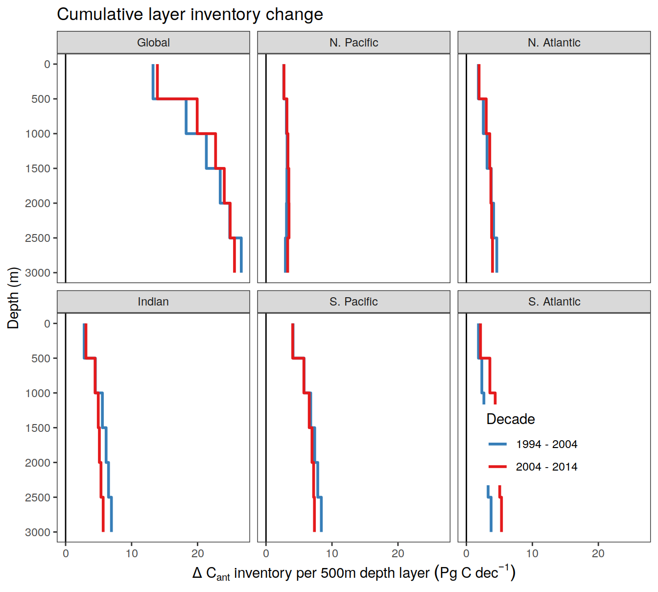
| Version | Author | Date |
|---|---|---|
| 3a7bab0 | jens-daniel-mueller | 2022-11-28 |
| ea34027 | jens-daniel-mueller | 2022-11-15 |
| 5520de8 | jens-daniel-mueller | 2022-11-15 |
| ebc85e2 | jens-daniel-mueller | 2022-11-14 |
| 2345935 | jens-daniel-mueller | 2022-10-29 |
| 91052ae | jens-daniel-mueller | 2022-10-20 |
| 78dbb27 | jens-daniel-mueller | 2022-08-11 |
| 302d289 | jens-daniel-mueller | 2022-08-11 |
| fea41c1 | jens-daniel-mueller | 2022-07-20 |
| d2ae54c | jens-daniel-mueller | 2022-07-18 |
| 2695085 | jens-daniel-mueller | 2022-07-17 |
| 26e9496 | jens-daniel-mueller | 2022-07-12 |
| 37f56b3 | jens-daniel-mueller | 2022-07-01 |
| df21d31 | jens-daniel-mueller | 2022-07-01 |
| 87e9eb8 | jens-daniel-mueller | 2022-06-27 |
| b52b159 | jens-daniel-mueller | 2022-06-27 |
| 1d73ec9 | jens-daniel-mueller | 2022-05-16 |
| 2ca0109 | jens-daniel-mueller | 2022-05-02 |
| b018a9a | jens-daniel-mueller | 2022-04-29 |
| e09320d | jens-daniel-mueller | 2022-04-12 |
| acad2e2 | jens-daniel-mueller | 2022-04-09 |
| 3d81135 | jens-daniel-mueller | 2022-04-07 |
| a74e341 | jens-daniel-mueller | 2022-04-04 |
| bd9e11d | jens-daniel-mueller | 2022-03-22 |
| 2501978 | jens-daniel-mueller | 2022-03-21 |
| d2191ad | jens-daniel-mueller | 2022-02-04 |
| 32e9682 | jens-daniel-mueller | 2022-02-02 |
| 913e42f | jens-daniel-mueller | 2022-02-01 |
| 189de95 | jens-daniel-mueller | 2022-02-01 |
| ab001eb | jens-daniel-mueller | 2022-01-31 |
| b62308d | jens-daniel-mueller | 2022-01-31 |
| 5f2aed0 | jens-daniel-mueller | 2022-01-27 |
15 Penetration depth
mean_column_inventory <- beta_budget_basin_MLR_all_ensemble %>%
mutate(dcant_area = dcant * 1e15 / 12 / area)
mean_column_inventory %>%
filter(period %in% two_decades,
data_source == "obs") %>%
ggplot(aes(x = period,
y = dcant_area,
fill = MLR_basins)) +
geom_jitter(shape = 21, alpha = 0.8) +
scale_fill_muted() +
facet_wrap(~basin)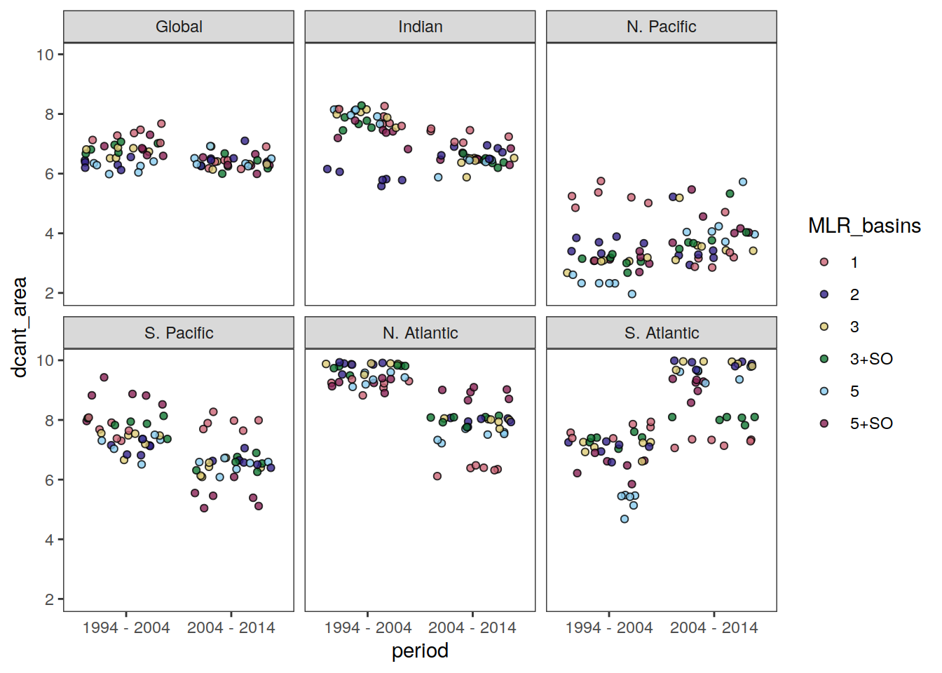
mean_surface_dcant %>%
filter(period %in% two_decades,
data_source == "obs") %>%
ggplot(aes(x = period,
y = mean_surface_dcant,
fill = MLR_basins)) +
geom_jitter(shape = 21, alpha = 0.8) +
scale_fill_muted() +
facet_wrap(~basin)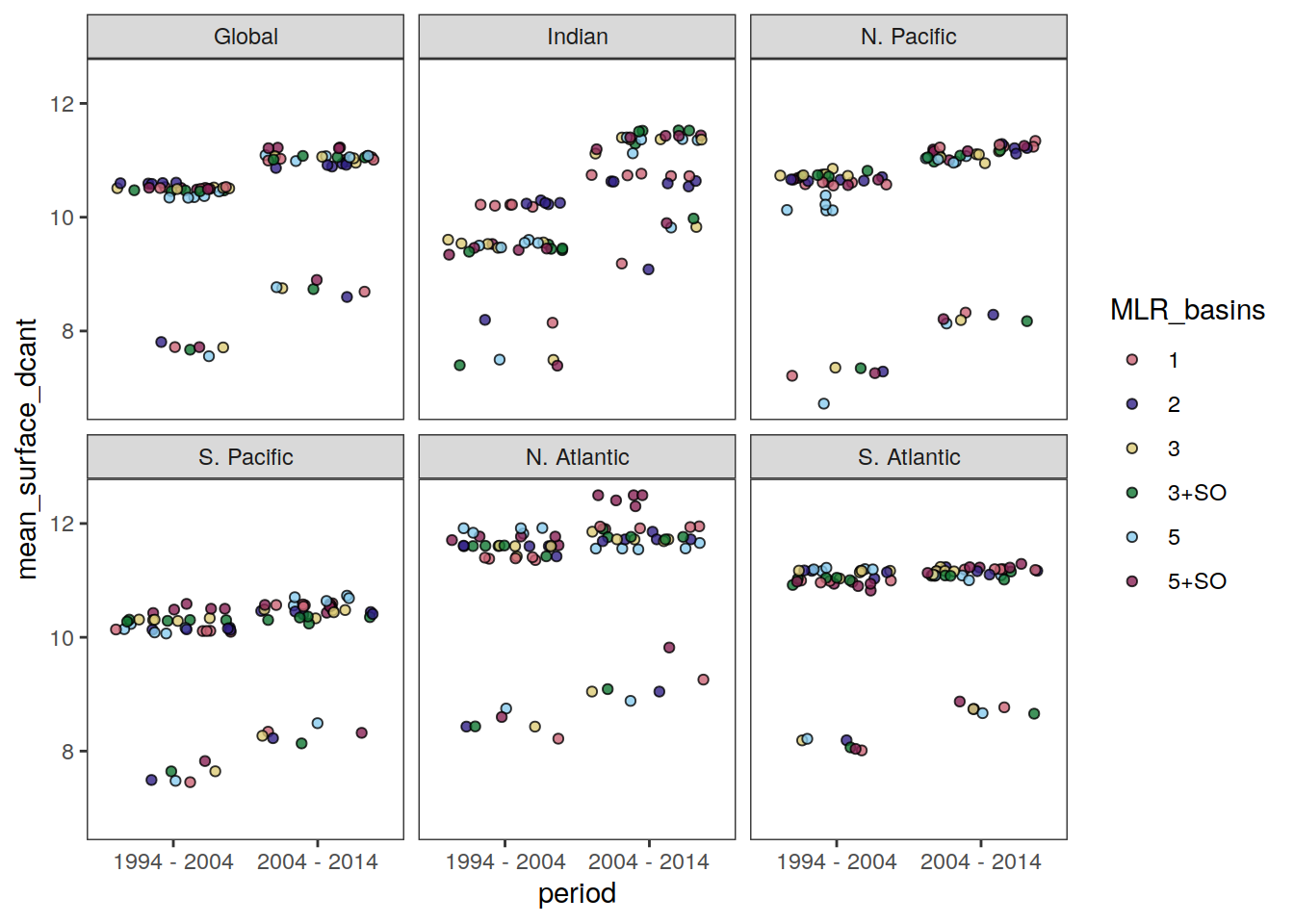
dcant_mean_penetration_depth <-
full_join(mean_column_inventory,
mean_surface_dcant) %>%
filter(Version_ID_group != "Surface eMLR(C*)") %>%
mutate(mean_surface_dcant = mean_surface_dcant * 1e3 * 1.025 / 1e6,
penetration_depth = dcant_area/mean_surface_dcant)
dcant_mean_penetration_depth %>%
filter(period %in% two_decades,
data_source == "obs") %>%
ggplot(aes(x = period,
y = penetration_depth,
fill = MLR_basins)) +
geom_jitter(shape = 21, alpha = 0.8) +
scale_fill_muted() +
facet_wrap(~basin)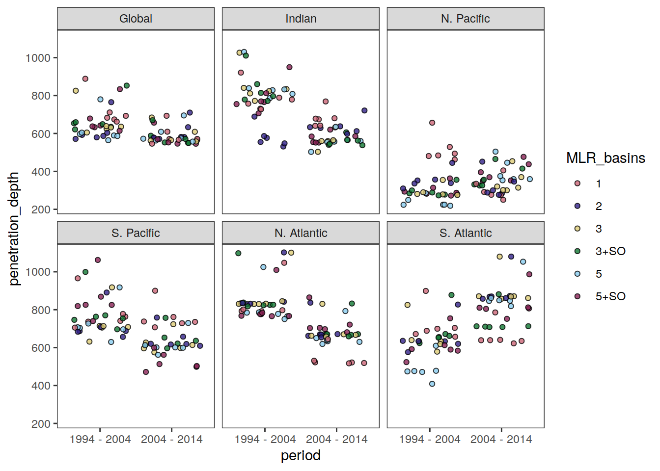
dcant_mean_penetration_depth_uncertainty <-
additive_uncertainty(
dcant_mean_penetration_depth %>%
filter(period %in% two_decades) %>%
select(data_source, period, Version_ID_group, MLR_basins, basin, penetration_depth) %>%
rename(dcant = penetration_depth))
delta_dcant_mean_penetration_depth_uncertainty <-
dcant_mean_penetration_depth_uncertainty[[3]]
dcant_mean_penetration_depth_uncertainty <-
dcant_mean_penetration_depth_uncertainty[[1]]
dcant_mean_penetration_depth_uncertainty %>%
filter(data_source == "obs") %>%
select(-c(data_source, starts_with("signif_"))) %>%
arrange(basin, period) %>%
kable() %>%
kable_styling() %>%
scroll_box(height = "300px")| period | basin | sd | std_case |
|---|---|---|---|
| 1994 - 2004 | Global | 195.1579 | 635.7219 |
| 2004 - 2014 | Global | 128.5704 | 564.4056 |
| 1994 - 2004 | Indian | 220.8476 | 834.0676 |
| 2004 - 2014 | Indian | 101.2224 | 559.8123 |
| 1994 - 2004 | N. Pacific | 100.3504 | 279.0525 |
| 2004 - 2014 | N. Pacific | 174.3395 | 300.0561 |
| 1994 - 2004 | S. Pacific | 227.9048 | 708.5043 |
| 2004 - 2014 | S. Pacific | 145.4462 | 596.1376 |
| 1994 - 2004 | N. Atlantic | 273.0824 | 829.9681 |
| 2004 - 2014 | N. Atlantic | 169.2454 | 668.0443 |
| 1994 - 2004 | S. Atlantic | 208.4508 | 633.5340 |
| 2004 - 2014 | S. Atlantic | 230.6747 | 870.9505 |
delta_dcant_mean_penetration_depth_uncertainty %>%
filter(data_source == "obs") %>%
select(-c(data_source, sd, std_case)) %>%
arrange(basin, period) %>%
kable() %>%
kable_styling() %>%
scroll_box(height = "300px")| period | basin | delta_dcant | RSS | signif_single | signif_double |
|---|---|---|---|---|---|
| 2004 - 2014 | Global | -71.31634 | 233.7027 | 0 | 0 |
| 2004 - 2014 | Indian | -274.25531 | 242.9396 | 1 | 0 |
| 2004 - 2014 | N. Pacific | 21.00356 | 201.1578 | 0 | 0 |
| 2004 - 2014 | S. Pacific | -112.36662 | 270.3612 | 0 | 0 |
| 2004 - 2014 | N. Atlantic | -161.92382 | 321.2756 | 0 | 0 |
| 2004 - 2014 | S. Atlantic | 237.41652 | 310.9060 | 0 | 0 |
dcant_mean_penetration_depth_uncertainty %>%
filter(period %in% two_decades,
data_source == "obs") %>%
ggplot(aes(x = basin,
y = std_case,
ymin = std_case - sd,
ymax = std_case + sd,
col = period)) +
scale_y_reverse(limits = c(1000,0)) +
geom_pointrange(position = position_dodge(width = 0.3))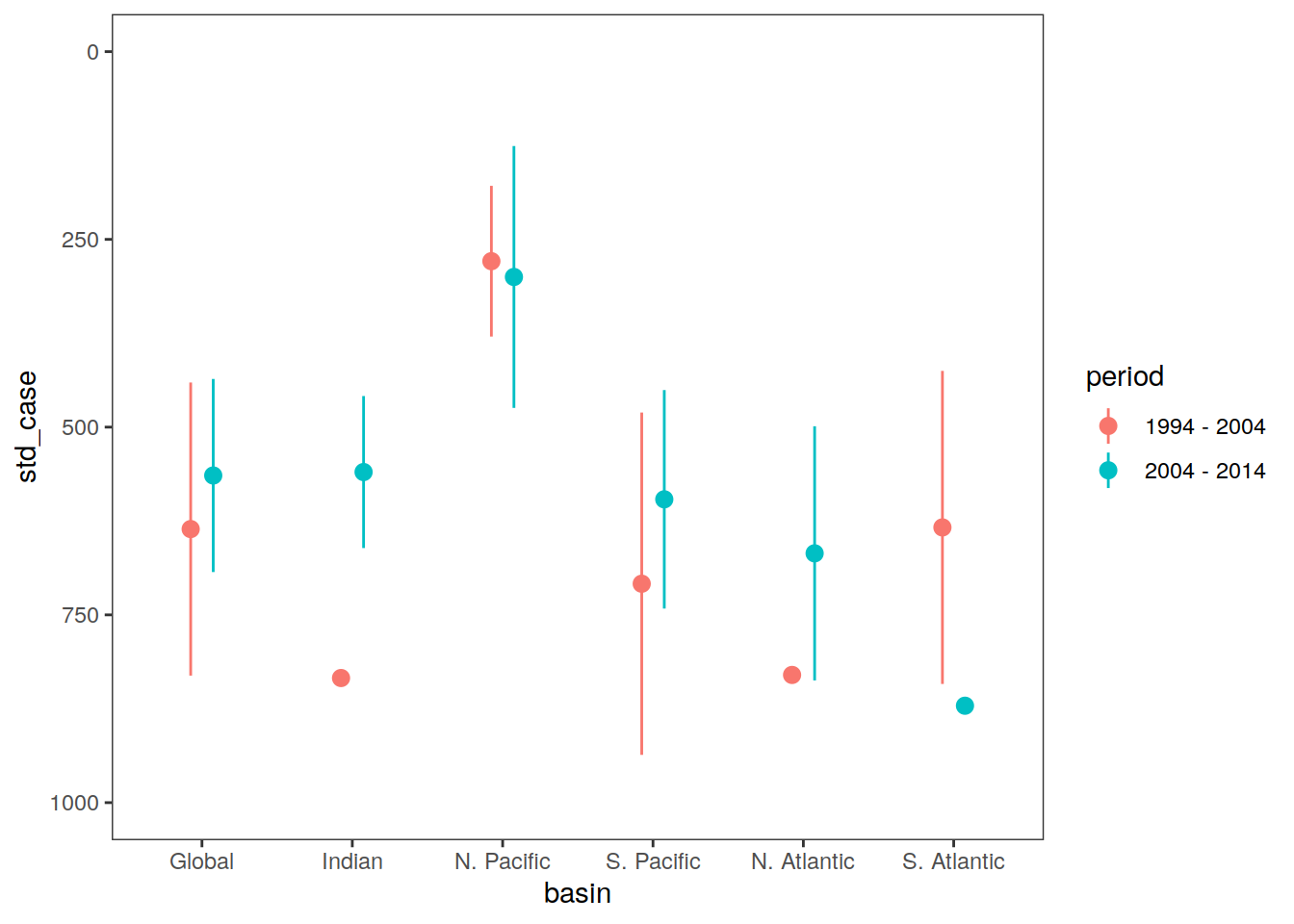
rm(mean_surface_dcant,
dcant_mean_penetration_depth,
dcant_mean_penetration_depth_uncertainty)16 Time series
16.1 eMLR only
dcant_budget_global_all_ensemble <-
dcant_budget_basin_MLR_all_ensemble %>%
filter(basin == "Global")
dcant_budget_global_all_ensemble %>%
filter(data_source == "obs",
period != "1994 - 2014") %>%
ggplot(aes(tref2, dcant, group = interaction(MLR_basins, Version_ID_group),
col=Version_ID_group)) +
geom_path() +
geom_point()
| Version | Author | Date |
|---|---|---|
| 8ded995 | jens-daniel-mueller | 2023-01-05 |
| 0f2c9d5 | jens-daniel-mueller | 2022-12-08 |
| 3a7bab0 | jens-daniel-mueller | 2022-11-28 |
| 534ee74 | jens-daniel-mueller | 2022-11-25 |
| 1dad51a | jens-daniel-mueller | 2022-11-15 |
| 6edad9b | jens-daniel-mueller | 2022-11-11 |
| 16beb51 | jens-daniel-mueller | 2022-11-08 |
| b92657d | jens-daniel-mueller | 2022-11-08 |
| 7275091 | jens-daniel-mueller | 2022-11-05 |
| 99610ed | jens-daniel-mueller | 2022-11-01 |
| 7060801 | jens-daniel-mueller | 2022-10-31 |
| ecb84c1 | jens-daniel-mueller | 2022-10-30 |
| 2345935 | jens-daniel-mueller | 2022-10-29 |
| 051b911 | jens-daniel-mueller | 2022-09-07 |
| 75bd58c | jens-daniel-mueller | 2022-09-07 |
| 1c6de0d | jens-daniel-mueller | 2022-09-07 |
| fea41c1 | jens-daniel-mueller | 2022-07-20 |
| d2ae54c | jens-daniel-mueller | 2022-07-18 |
| 2695085 | jens-daniel-mueller | 2022-07-17 |
| 535196a | jens-daniel-mueller | 2022-07-17 |
| d20faeb | jens-daniel-mueller | 2022-07-17 |
| afb27ad | jens-daniel-mueller | 2022-07-15 |
| b492b46 | jens-daniel-mueller | 2022-07-15 |
| bd24a0f | jens-daniel-mueller | 2022-07-15 |
| 17cd1d1 | jens-daniel-mueller | 2022-07-13 |
| 8fb595c | jens-daniel-mueller | 2022-07-12 |
| 003b161 | jens-daniel-mueller | 2022-07-12 |
| 232909e | jens-daniel-mueller | 2022-07-01 |
dcant_budget_global_all_ensemble %>%
filter(data_source == "obs") %>%
select(MLR_basins, Version_ID_group, period, dcant) %>%
pivot_wider(names_from = period,
values_from = dcant) %>%
ggplot(aes(`1994 - 2004`, `2004 - 2014`,
col=MLR_basins)) +
coord_equal() +
geom_point() +
facet_wrap(~ Version_ID_group)
| Version | Author | Date |
|---|---|---|
| 8ded995 | jens-daniel-mueller | 2023-01-05 |
| 0f2c9d5 | jens-daniel-mueller | 2022-12-08 |
| 3a7bab0 | jens-daniel-mueller | 2022-11-28 |
| 534ee74 | jens-daniel-mueller | 2022-11-25 |
| 1dad51a | jens-daniel-mueller | 2022-11-15 |
| 6edad9b | jens-daniel-mueller | 2022-11-11 |
| 16beb51 | jens-daniel-mueller | 2022-11-08 |
| b92657d | jens-daniel-mueller | 2022-11-08 |
| 7275091 | jens-daniel-mueller | 2022-11-05 |
| 99610ed | jens-daniel-mueller | 2022-11-01 |
| 7060801 | jens-daniel-mueller | 2022-10-31 |
| ecb84c1 | jens-daniel-mueller | 2022-10-30 |
| 2345935 | jens-daniel-mueller | 2022-10-29 |
| 051b911 | jens-daniel-mueller | 2022-09-07 |
| 75bd58c | jens-daniel-mueller | 2022-09-07 |
| 1c6de0d | jens-daniel-mueller | 2022-09-07 |
| fea41c1 | jens-daniel-mueller | 2022-07-20 |
| b1f7ab3 | jens-daniel-mueller | 2022-07-18 |
| d2ae54c | jens-daniel-mueller | 2022-07-18 |
| 2695085 | jens-daniel-mueller | 2022-07-17 |
| 535196a | jens-daniel-mueller | 2022-07-17 |
| d20faeb | jens-daniel-mueller | 2022-07-17 |
| afb27ad | jens-daniel-mueller | 2022-07-15 |
| b492b46 | jens-daniel-mueller | 2022-07-15 |
| bd24a0f | jens-daniel-mueller | 2022-07-15 |
| 17cd1d1 | jens-daniel-mueller | 2022-07-13 |
| 8fb595c | jens-daniel-mueller | 2022-07-12 |
| 003b161 | jens-daniel-mueller | 2022-07-12 |
| 232909e | jens-daniel-mueller | 2022-07-01 |
dcant_budget_global_all_ensemble %>%
filter(data_source == "obs") %>%
select(MLR_basins, Version_ID_group, period, dcant) %>%
pivot_wider(names_from = period,
values_from = dcant) %>%
ggplot(aes(`1994 - 2004`, `2004 - 2014`,
col=Version_ID_group)) +
coord_equal() +
geom_point() +
facet_wrap(~ MLR_basins)
| Version | Author | Date |
|---|---|---|
| 8ded995 | jens-daniel-mueller | 2023-01-05 |
| 0f2c9d5 | jens-daniel-mueller | 2022-12-08 |
| 3a7bab0 | jens-daniel-mueller | 2022-11-28 |
| 534ee74 | jens-daniel-mueller | 2022-11-25 |
| 1dad51a | jens-daniel-mueller | 2022-11-15 |
| 6edad9b | jens-daniel-mueller | 2022-11-11 |
| 16beb51 | jens-daniel-mueller | 2022-11-08 |
| b92657d | jens-daniel-mueller | 2022-11-08 |
| 7275091 | jens-daniel-mueller | 2022-11-05 |
| 99610ed | jens-daniel-mueller | 2022-11-01 |
| 7060801 | jens-daniel-mueller | 2022-10-31 |
| ecb84c1 | jens-daniel-mueller | 2022-10-30 |
| 2345935 | jens-daniel-mueller | 2022-10-29 |
| 051b911 | jens-daniel-mueller | 2022-09-07 |
| 75bd58c | jens-daniel-mueller | 2022-09-07 |
| 1c6de0d | jens-daniel-mueller | 2022-09-07 |
| fea41c1 | jens-daniel-mueller | 2022-07-20 |
| b1f7ab3 | jens-daniel-mueller | 2022-07-18 |
| d2ae54c | jens-daniel-mueller | 2022-07-18 |
| 2695085 | jens-daniel-mueller | 2022-07-17 |
| 535196a | jens-daniel-mueller | 2022-07-17 |
| d20faeb | jens-daniel-mueller | 2022-07-17 |
| afb27ad | jens-daniel-mueller | 2022-07-15 |
| b492b46 | jens-daniel-mueller | 2022-07-15 |
| bd24a0f | jens-daniel-mueller | 2022-07-15 |
| 17cd1d1 | jens-daniel-mueller | 2022-07-13 |
| 8fb595c | jens-daniel-mueller | 2022-07-12 |
| 003b161 | jens-daniel-mueller | 2022-07-12 |
| 232909e | jens-daniel-mueller | 2022-07-01 |
dcant_budget_global_all_ensemble %>%
filter(data_source == "obs") %>%
select(MLR_basins, Version_ID_group, period, dcant) %>%
pivot_wider(names_from = period,
values_from = dcant) %>%
ggplot(aes(`1994 - 2004`, `1994 - 2014`,
col=Version_ID_group)) +
coord_equal() +
geom_point()
| Version | Author | Date |
|---|---|---|
| 8ded995 | jens-daniel-mueller | 2023-01-05 |
| 0f2c9d5 | jens-daniel-mueller | 2022-12-08 |
| 3a7bab0 | jens-daniel-mueller | 2022-11-28 |
| 534ee74 | jens-daniel-mueller | 2022-11-25 |
| 1dad51a | jens-daniel-mueller | 2022-11-15 |
| 6edad9b | jens-daniel-mueller | 2022-11-11 |
| 16beb51 | jens-daniel-mueller | 2022-11-08 |
| b92657d | jens-daniel-mueller | 2022-11-08 |
| 7275091 | jens-daniel-mueller | 2022-11-05 |
| 99610ed | jens-daniel-mueller | 2022-11-01 |
| 7060801 | jens-daniel-mueller | 2022-10-31 |
| ecb84c1 | jens-daniel-mueller | 2022-10-30 |
| 2345935 | jens-daniel-mueller | 2022-10-29 |
| 051b911 | jens-daniel-mueller | 2022-09-07 |
| 75bd58c | jens-daniel-mueller | 2022-09-07 |
| 1c6de0d | jens-daniel-mueller | 2022-09-07 |
| fea41c1 | jens-daniel-mueller | 2022-07-20 |
| b1f7ab3 | jens-daniel-mueller | 2022-07-18 |
| d2ae54c | jens-daniel-mueller | 2022-07-18 |
| 2695085 | jens-daniel-mueller | 2022-07-17 |
| 535196a | jens-daniel-mueller | 2022-07-17 |
| d20faeb | jens-daniel-mueller | 2022-07-17 |
| afb27ad | jens-daniel-mueller | 2022-07-15 |
| b492b46 | jens-daniel-mueller | 2022-07-15 |
| bd24a0f | jens-daniel-mueller | 2022-07-15 |
| 17cd1d1 | jens-daniel-mueller | 2022-07-13 |
| 8fb595c | jens-daniel-mueller | 2022-07-12 |
| 003b161 | jens-daniel-mueller | 2022-07-12 |
| 232909e | jens-daniel-mueller | 2022-07-01 |
dcant_budget_global_all_ensemble %>%
filter(data_source == "obs") %>%
select(MLR_basins, Version_ID_group, period, dcant) %>%
pivot_wider(names_from = period,
values_from = dcant) %>%
ggplot(aes(`1994 - 2004` + `2004 - 2014`, `1994 - 2014`,
col=Version_ID_group)) +
geom_abline(intercept = 0, slope = 1) +
coord_equal() +
scale_x_continuous(breaks = seq(0,100,1)) +
scale_y_continuous(breaks = seq(0,100,1)) +
geom_point()
| Version | Author | Date |
|---|---|---|
| 8ded995 | jens-daniel-mueller | 2023-01-05 |
| 0f2c9d5 | jens-daniel-mueller | 2022-12-08 |
| 3a7bab0 | jens-daniel-mueller | 2022-11-28 |
| 534ee74 | jens-daniel-mueller | 2022-11-25 |
| 1dad51a | jens-daniel-mueller | 2022-11-15 |
| 6edad9b | jens-daniel-mueller | 2022-11-11 |
| 16beb51 | jens-daniel-mueller | 2022-11-08 |
| b92657d | jens-daniel-mueller | 2022-11-08 |
| 7275091 | jens-daniel-mueller | 2022-11-05 |
| 99610ed | jens-daniel-mueller | 2022-11-01 |
| 7060801 | jens-daniel-mueller | 2022-10-31 |
| ecb84c1 | jens-daniel-mueller | 2022-10-30 |
| 2345935 | jens-daniel-mueller | 2022-10-29 |
| 051b911 | jens-daniel-mueller | 2022-09-07 |
| 75bd58c | jens-daniel-mueller | 2022-09-07 |
| 1c6de0d | jens-daniel-mueller | 2022-09-07 |
| fea41c1 | jens-daniel-mueller | 2022-07-20 |
| b1f7ab3 | jens-daniel-mueller | 2022-07-18 |
dcant_budget_global_ts <- dcant_budget_basin_MLR_all %>%
filter(basin == "Global",
data_source == "obs",
period %in% two_decades) %>%
select(year = tref2, dcant_mean = dcant)
dcant_budget_global_all_ensemble_summary <-
dcant_budget_basin_MLR_all_uncertainty %>%
filter(data_source == "obs",
basin == "Global") %>%
mutate(
tref2 = as.numeric(str_sub(period, 8, 11)),
dcant_sd = sqrt(sd ^ 2 + lag(sd, default = 0) ^ 2),
dcant_sd_int = sd
) %>%
select(data_source, tref2, dcant_sd, dcant_sd_int)
# dcant_budget_global_all_ensemble_summary <-
# dcant_budget_basin_MLR_all_uncertainty_two_decades %>%
# filter(period %in% c("1994 - 2004", "1994 - 2014"),
# data_source == "obs",
# basin == "Global") %>%
# select(data_source, tref2, period, sd) %>%
# mutate(dcant_sd = sd*sd_factor)
# dcant_budget_global_all_ensemble_summary <-
# dcant_budget_basin_MLR_all_ensemble %>%
# filter(period %in% c("1994 - 2004", "1994 - 2014"),
# data_source == "obs",
# basin == "Global") %>%
# group_by(data_source, tref2, period) %>%
# summarise(#dcant_mean = mean(dcant),
# dcant_sd = sd(dcant)*sd_factor) %>%
# ungroup()
dcant_budget_global_ts <- left_join(dcant_budget_global_ts,
dcant_budget_global_all_ensemble_summary %>%
select(year = tref2, dcant_sd, dcant_sd_int))
tcant_S04 <- bind_cols(year = 1994, dcant_mean = 118, dcant_sd = 19)
tcant_ts <- full_join(dcant_budget_global_ts, tcant_S04)
tcant_ts <- left_join(tcant_ts, co2_atm)
co2_atm_pi <- bind_cols(pCO2 = 280, dcant_mean = 0, year = 1800, dcant_sd = NA)
tcant_ts <- full_join(tcant_ts, co2_atm_pi)
tcant_ts <- tcant_ts %>%
arrange(year) %>%
mutate(
tcant = cumsum(dcant_mean),
tcant_sd = sqrt(dcant_sd ^ 2 + nth(dcant_sd,2) ^ 2)
) %>%
mutate(
tcant_sd = case_when(
year == 1800 ~ 0,
year == 1994 ~ dcant_sd,
TRUE ~ tcant_sd
),
dcant_sd_int = case_when(
year == 1994 ~ dcant_sd,
TRUE ~ dcant_sd_int
),
dcant_sd = case_when(
year == 1994 ~ 0,
TRUE ~ dcant_sd
)
)
beta <- 1.57
co2_atm_pi_value <- 283
atm_co2_col <- "#CC3311"
tcant_col <- "#004488"
p_tcant_year <- tcant_ts %>%
ggplot(aes(year, tcant)) +
geom_line(data = co2_atm_reccap2 %>% filter(year > 1790),
aes(year, (pCO2 - co2_atm_pi_value) * beta),
col = atm_co2_col) +
geom_linerange(data = tcant_ts %>% filter(year != 1994),
aes(
ymin = tcant - dcant_sd_int*2,
ymax = tcant + dcant_sd_int*2,
col = "Central estimate\n \u00B1 1σ/2σ uncertainty"
), linewidth = 0.5) +
geom_linerange(aes(
ymin = tcant - dcant_sd_int,
ymax = tcant + dcant_sd_int,
col = "Central estimate\n \u00B1 1σ/2σ uncertainty"
), linewidth = 1) +
geom_point(fill = "white", shape = 21,
aes(col = "Central estimate\n \u00B1 1σ/2σ uncertainty")) +
scale_y_continuous(name = expression(Total ~ oceanic ~ C[ant] ~ (Pg~C)),
sec.axis = sec_axis( ~ (. / beta + co2_atm_pi_value),
name = expression(Atm. ~ pCO[2] ~ (µatm)))) +
scale_x_continuous(name = "Year", breaks = seq(1800, 2000, 50)) +
scale_color_manual(values = tcant_col) +
theme(
axis.title.y.right = element_text(color = atm_co2_col),
axis.text.y.right = element_text(color = atm_co2_col),
axis.ticks.y.right = element_line(color = atm_co2_col),
axis.title.y.left = element_text(color = tcant_col),
axis.text.y.left = element_text(color = tcant_col),
axis.ticks.y.left = element_line(color = tcant_col),
legend.background = element_rect(fill = "transparent"),
legend.position = c(0.85, 0.2),
legend.title = element_blank()
)
p_tcant_year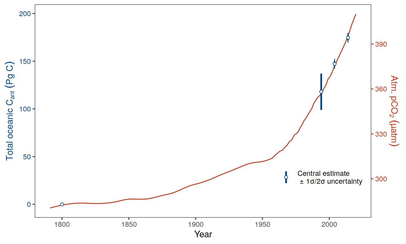
| Version | Author | Date |
|---|---|---|
| 2cca4eb | jens-daniel-mueller | 2023-01-10 |
| 0f2c9d5 | jens-daniel-mueller | 2022-12-08 |
| 3a7bab0 | jens-daniel-mueller | 2022-11-28 |
| 322b1c1 | jens-daniel-mueller | 2022-11-25 |
| 491f8b1 | jens-daniel-mueller | 2022-11-25 |
| 4da4d66 | jens-daniel-mueller | 2022-11-25 |
| 534ee74 | jens-daniel-mueller | 2022-11-25 |
| e924c80 | jens-daniel-mueller | 2022-11-17 |
| ea34027 | jens-daniel-mueller | 2022-11-15 |
| 1dad51a | jens-daniel-mueller | 2022-11-15 |
| 375300e | jens-daniel-mueller | 2022-11-14 |
| 6edad9b | jens-daniel-mueller | 2022-11-11 |
| 16beb51 | jens-daniel-mueller | 2022-11-08 |
| b92657d | jens-daniel-mueller | 2022-11-08 |
| 7275091 | jens-daniel-mueller | 2022-11-05 |
| 99610ed | jens-daniel-mueller | 2022-11-01 |
| 7060801 | jens-daniel-mueller | 2022-10-31 |
| ecb84c1 | jens-daniel-mueller | 2022-10-30 |
| 2345935 | jens-daniel-mueller | 2022-10-29 |
| 91052ae | jens-daniel-mueller | 2022-10-20 |
| 051b911 | jens-daniel-mueller | 2022-09-07 |
| 75bd58c | jens-daniel-mueller | 2022-09-07 |
| 1c6de0d | jens-daniel-mueller | 2022-09-07 |
| 78dbb27 | jens-daniel-mueller | 2022-08-11 |
| 302d289 | jens-daniel-mueller | 2022-08-11 |
| 9bbc6a4 | jens-daniel-mueller | 2022-07-20 |
| fea41c1 | jens-daniel-mueller | 2022-07-20 |
| d803308 | jens-daniel-mueller | 2022-07-19 |
| b1f7ab3 | jens-daniel-mueller | 2022-07-18 |
| d2ae54c | jens-daniel-mueller | 2022-07-18 |
| 2695085 | jens-daniel-mueller | 2022-07-17 |
| 535196a | jens-daniel-mueller | 2022-07-17 |
| afb27ad | jens-daniel-mueller | 2022-07-15 |
| b492b46 | jens-daniel-mueller | 2022-07-15 |
| bd24a0f | jens-daniel-mueller | 2022-07-15 |
| 17cd1d1 | jens-daniel-mueller | 2022-07-13 |
| 8fb595c | jens-daniel-mueller | 2022-07-12 |
| 003b161 | jens-daniel-mueller | 2022-07-12 |
| 8ab4a87 | jens-daniel-mueller | 2022-06-29 |
| 7629c78 | jens-daniel-mueller | 2022-06-29 |
| f6786c8 | jens-daniel-mueller | 2022-06-29 |
| 0825298 | jens-daniel-mueller | 2022-06-28 |
| 87e9eb8 | jens-daniel-mueller | 2022-06-27 |
| b52b159 | jens-daniel-mueller | 2022-06-27 |
| 1d73ec9 | jens-daniel-mueller | 2022-05-16 |
| 2ca0109 | jens-daniel-mueller | 2022-05-02 |
| b018a9a | jens-daniel-mueller | 2022-04-29 |
| e09320d | jens-daniel-mueller | 2022-04-12 |
| 8dca96a | jens-daniel-mueller | 2022-04-12 |
| 209c9b6 | jens-daniel-mueller | 2022-04-10 |
| acad2e2 | jens-daniel-mueller | 2022-04-09 |
| 3d81135 | jens-daniel-mueller | 2022-04-07 |
| a74e341 | jens-daniel-mueller | 2022-04-04 |
| 5a6be34 | jens-daniel-mueller | 2022-03-22 |
| bd9e11d | jens-daniel-mueller | 2022-03-22 |
| 2501978 | jens-daniel-mueller | 2022-03-21 |
| 251c7cf | jens-daniel-mueller | 2022-02-17 |
| 565224d | jens-daniel-mueller | 2022-02-17 |
| 2116dd3 | jens-daniel-mueller | 2022-02-09 |
| 6fe70a1 | jens-daniel-mueller | 2022-02-05 |
| a6b33aa | jens-daniel-mueller | 2022-02-04 |
atm_co2_col <- "transparent"
p_tcant_year_trans <- tcant_ts %>%
ggplot(aes(year, tcant)) +
geom_line(data = co2_atm_reccap2 %>% filter(year > 1790),
aes(year, (pCO2 - co2_atm_pi_value) * beta),
col = atm_co2_col) +
geom_linerange(data = tcant_ts %>% filter(year != 1994),
aes(
ymin = tcant - dcant_sd_int*2,
ymax = tcant + dcant_sd_int*2,
col = "Central estimate\n \u00B1 1σ/2σ uncertainty"
), linewidth = 0.5) +
geom_linerange(aes(
ymin = tcant - dcant_sd_int,
ymax = tcant + dcant_sd_int,
col = "Central estimate\n \u00B1 1σ/2σ uncertainty"
), linewidth = 1) +
geom_point(fill = "white", shape = 21,
aes(col = "Central estimate\n \u00B1 1σ/2σ uncertainty")) +
scale_y_continuous(name = expression(Total ~ oceanic ~ C[ant] ~ (Pg~C)),
sec.axis = sec_axis( ~ (. / beta + co2_atm_pi_value),
name = expression(Atm. ~ pCO[2] ~ (µatm)))) +
scale_x_continuous(name = "Year", breaks = seq(1800, 2000, 50)) +
scale_color_manual(values = tcant_col) +
theme(
axis.title.y.right = element_text(color = atm_co2_col),
axis.text.y.right = element_text(color = atm_co2_col),
axis.ticks.y.right = element_line(color = atm_co2_col),
axis.title.y.left = element_text(color = tcant_col),
axis.text.y.left = element_text(color = tcant_col),
axis.ticks.y.left = element_line(color = tcant_col),
legend.background = element_rect(fill = "transparent"),
legend.position = c(0.85, 0.2),
legend.title = element_blank()
)
p_tcant_year_trans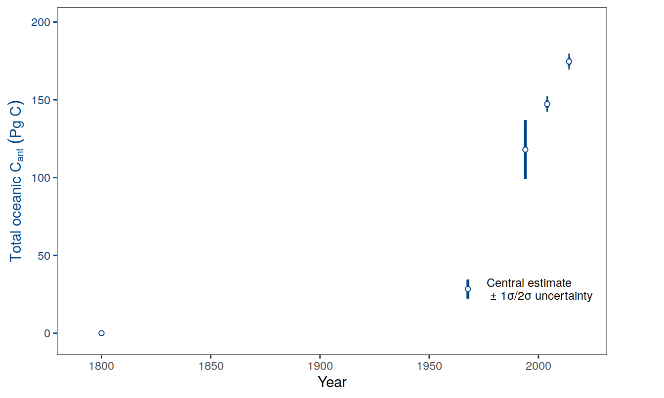
| Version | Author | Date |
|---|---|---|
| fdf5f22 | jens-daniel-mueller | 2023-01-11 |
| 2cca4eb | jens-daniel-mueller | 2023-01-10 |
| 3a7bab0 | jens-daniel-mueller | 2022-11-28 |
| 322b1c1 | jens-daniel-mueller | 2022-11-25 |
| 491f8b1 | jens-daniel-mueller | 2022-11-25 |
| 4da4d66 | jens-daniel-mueller | 2022-11-25 |
| 534ee74 | jens-daniel-mueller | 2022-11-25 |
| e924c80 | jens-daniel-mueller | 2022-11-17 |
| ea34027 | jens-daniel-mueller | 2022-11-15 |
| 1dad51a | jens-daniel-mueller | 2022-11-15 |
| 375300e | jens-daniel-mueller | 2022-11-14 |
| 6edad9b | jens-daniel-mueller | 2022-11-11 |
| 16beb51 | jens-daniel-mueller | 2022-11-08 |
| b92657d | jens-daniel-mueller | 2022-11-08 |
| 7275091 | jens-daniel-mueller | 2022-11-05 |
| 99610ed | jens-daniel-mueller | 2022-11-01 |
| 7060801 | jens-daniel-mueller | 2022-10-31 |
| ecb84c1 | jens-daniel-mueller | 2022-10-30 |
| 2345935 | jens-daniel-mueller | 2022-10-29 |
| 91052ae | jens-daniel-mueller | 2022-10-20 |
| d803308 | jens-daniel-mueller | 2022-07-19 |
| b1f7ab3 | jens-daniel-mueller | 2022-07-18 |
| d2ae54c | jens-daniel-mueller | 2022-07-18 |
| 2695085 | jens-daniel-mueller | 2022-07-17 |
| 535196a | jens-daniel-mueller | 2022-07-17 |
| afb27ad | jens-daniel-mueller | 2022-07-15 |
| b492b46 | jens-daniel-mueller | 2022-07-15 |
| bd24a0f | jens-daniel-mueller | 2022-07-15 |
| 17cd1d1 | jens-daniel-mueller | 2022-07-13 |
| 8fb595c | jens-daniel-mueller | 2022-07-12 |
| 003b161 | jens-daniel-mueller | 2022-07-12 |
| 8ab4a87 | jens-daniel-mueller | 2022-06-29 |
| 7629c78 | jens-daniel-mueller | 2022-06-29 |
| f6786c8 | jens-daniel-mueller | 2022-06-29 |
| 0825298 | jens-daniel-mueller | 2022-06-28 |
| 87e9eb8 | jens-daniel-mueller | 2022-06-27 |
| b52b159 | jens-daniel-mueller | 2022-06-27 |
| 1d73ec9 | jens-daniel-mueller | 2022-05-16 |
| 2ca0109 | jens-daniel-mueller | 2022-05-02 |
| b018a9a | jens-daniel-mueller | 2022-04-29 |
| e09320d | jens-daniel-mueller | 2022-04-12 |
| 8dca96a | jens-daniel-mueller | 2022-04-12 |
| 209c9b6 | jens-daniel-mueller | 2022-04-10 |
| acad2e2 | jens-daniel-mueller | 2022-04-09 |
| 3d81135 | jens-daniel-mueller | 2022-04-07 |
| a74e341 | jens-daniel-mueller | 2022-04-04 |
| 5a6be34 | jens-daniel-mueller | 2022-03-22 |
| bd9e11d | jens-daniel-mueller | 2022-03-22 |
| 2501978 | jens-daniel-mueller | 2022-03-21 |
| 251c7cf | jens-daniel-mueller | 2022-02-17 |
| 565224d | jens-daniel-mueller | 2022-02-17 |
| 2116dd3 | jens-daniel-mueller | 2022-02-09 |
atm_co2_col <- "#CC3311"
p_tcant_atm_co2 <- tcant_ts %>%
ggplot(aes(pCO2, tcant)) +
geom_ribbon(aes(
ymin = tcant - tcant_sd,
ymax = tcant + tcant_sd,
fill = "1800 - 2014",
alpha = "1800 - 2014"
)) +
geom_ribbon(aes(
ymin = tcant - dcant_sd,
ymax = tcant + dcant_sd,
fill = "1994 - 2014",
alpha = "1994 - 2014"
)) +
geom_line(color = tcant_col) +
geom_point(shape = 21, fill = "white", color = tcant_col) +
scale_x_continuous(breaks = seq(280, 400, 30)) +
scale_fill_manual(values = c(tcant_col, tcant_col), name = "Cumulative\n1σ-uncertainty") +
scale_alpha_manual(values = c(0.2, 0.6), name = "Cumulative\n1σ-uncertainty") +
geom_text(aes(label = year), nudge_x = -6, nudge_y = 6) +
labs(x = expression(Atmospheric ~ pCO[2] ~ (µatm)),
y = expression(Total ~ oceanic ~ C[ant] ~ (Pg~C))) +
theme(
axis.title.y.left = element_text(color = tcant_col),
axis.text.y.left = element_text(color = tcant_col),
axis.ticks.y.left = element_line(color = tcant_col),
legend.background = element_rect(fill = "transparent"),
legend.position = c(0.85, 0.25),
axis.title.x = element_text(color = atm_co2_col),
axis.text.x = element_text(color = atm_co2_col),
axis.ticks.x = element_line(color = atm_co2_col)
)
p_tcant_year / p_tcant_atm_co2 +
plot_annotation(tag_levels = 'A')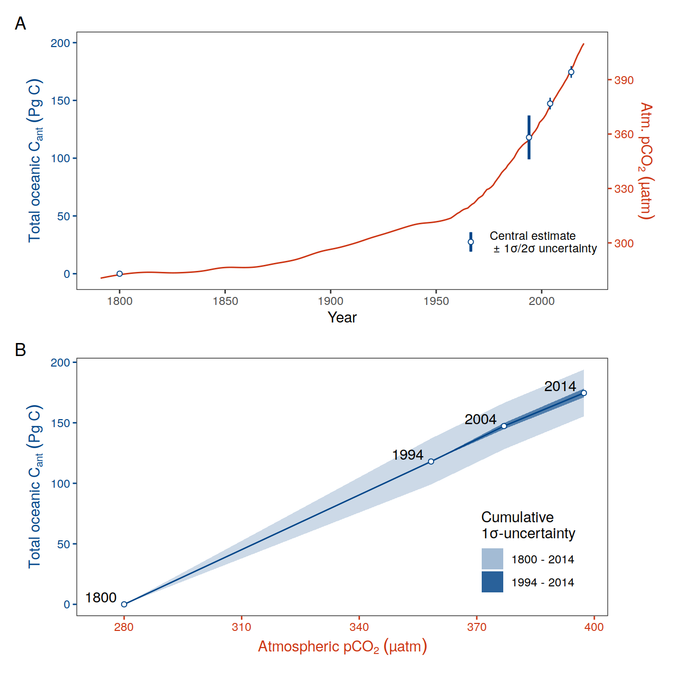
| Version | Author | Date |
|---|---|---|
| 2cca4eb | jens-daniel-mueller | 2023-01-10 |
| 0f2c9d5 | jens-daniel-mueller | 2022-12-08 |
| 3a7bab0 | jens-daniel-mueller | 2022-11-28 |
| 322b1c1 | jens-daniel-mueller | 2022-11-25 |
| 491f8b1 | jens-daniel-mueller | 2022-11-25 |
| 4da4d66 | jens-daniel-mueller | 2022-11-25 |
| 534ee74 | jens-daniel-mueller | 2022-11-25 |
| e924c80 | jens-daniel-mueller | 2022-11-17 |
| ea34027 | jens-daniel-mueller | 2022-11-15 |
| 1dad51a | jens-daniel-mueller | 2022-11-15 |
| 375300e | jens-daniel-mueller | 2022-11-14 |
| 6edad9b | jens-daniel-mueller | 2022-11-11 |
| 16beb51 | jens-daniel-mueller | 2022-11-08 |
| b92657d | jens-daniel-mueller | 2022-11-08 |
| 7275091 | jens-daniel-mueller | 2022-11-05 |
| 99610ed | jens-daniel-mueller | 2022-11-01 |
| 7060801 | jens-daniel-mueller | 2022-10-31 |
| ecb84c1 | jens-daniel-mueller | 2022-10-30 |
| 2345935 | jens-daniel-mueller | 2022-10-29 |
| 91052ae | jens-daniel-mueller | 2022-10-20 |
| 051b911 | jens-daniel-mueller | 2022-09-07 |
| 75bd58c | jens-daniel-mueller | 2022-09-07 |
| 1c6de0d | jens-daniel-mueller | 2022-09-07 |
| 78dbb27 | jens-daniel-mueller | 2022-08-11 |
| 302d289 | jens-daniel-mueller | 2022-08-11 |
| 9bbc6a4 | jens-daniel-mueller | 2022-07-20 |
| a80b59b | jens-daniel-mueller | 2022-07-20 |
| fea41c1 | jens-daniel-mueller | 2022-07-20 |
| d803308 | jens-daniel-mueller | 2022-07-19 |
| b1f7ab3 | jens-daniel-mueller | 2022-07-18 |
| d2ae54c | jens-daniel-mueller | 2022-07-18 |
| 2695085 | jens-daniel-mueller | 2022-07-17 |
| 535196a | jens-daniel-mueller | 2022-07-17 |
| afb27ad | jens-daniel-mueller | 2022-07-15 |
| b492b46 | jens-daniel-mueller | 2022-07-15 |
| bd24a0f | jens-daniel-mueller | 2022-07-15 |
| 17cd1d1 | jens-daniel-mueller | 2022-07-13 |
| 8fb595c | jens-daniel-mueller | 2022-07-12 |
| 003b161 | jens-daniel-mueller | 2022-07-12 |
| 8ab4a87 | jens-daniel-mueller | 2022-06-29 |
| 7629c78 | jens-daniel-mueller | 2022-06-29 |
| f6786c8 | jens-daniel-mueller | 2022-06-29 |
| 0825298 | jens-daniel-mueller | 2022-06-28 |
| 87e9eb8 | jens-daniel-mueller | 2022-06-27 |
| b52b159 | jens-daniel-mueller | 2022-06-27 |
| 1d73ec9 | jens-daniel-mueller | 2022-05-16 |
| 2ca0109 | jens-daniel-mueller | 2022-05-02 |
| b018a9a | jens-daniel-mueller | 2022-04-29 |
| e09320d | jens-daniel-mueller | 2022-04-12 |
| 8dca96a | jens-daniel-mueller | 2022-04-12 |
| 209c9b6 | jens-daniel-mueller | 2022-04-10 |
| acad2e2 | jens-daniel-mueller | 2022-04-09 |
| 3d81135 | jens-daniel-mueller | 2022-04-07 |
| a74e341 | jens-daniel-mueller | 2022-04-04 |
| 5a6be34 | jens-daniel-mueller | 2022-03-22 |
| bd9e11d | jens-daniel-mueller | 2022-03-22 |
| 2501978 | jens-daniel-mueller | 2022-03-21 |
| 251c7cf | jens-daniel-mueller | 2022-02-17 |
| 565224d | jens-daniel-mueller | 2022-02-17 |
| 2116dd3 | jens-daniel-mueller | 2022-02-09 |
| 6fe70a1 | jens-daniel-mueller | 2022-02-05 |
| a6b33aa | jens-daniel-mueller | 2022-02-04 |
| d2191ad | jens-daniel-mueller | 2022-02-04 |
| 0d0f790 | jens-daniel-mueller | 2022-02-02 |
| 60727e6 | jens-daniel-mueller | 2022-02-02 |
| c7b4984 | jens-daniel-mueller | 2022-02-02 |
| 7fb28a2 | jens-daniel-mueller | 2022-02-02 |
| 7655085 | jens-daniel-mueller | 2022-02-02 |
| ec7fe7e | jens-daniel-mueller | 2022-01-31 |
ggsave(path = here::here("output/publication"),
filename = "Fig_dcant_inventory_global_vs_atm_pCO2.png",
height = 6,
width = 7,
dpi = 600)
p_tcant_year / p_tcant_atm_co2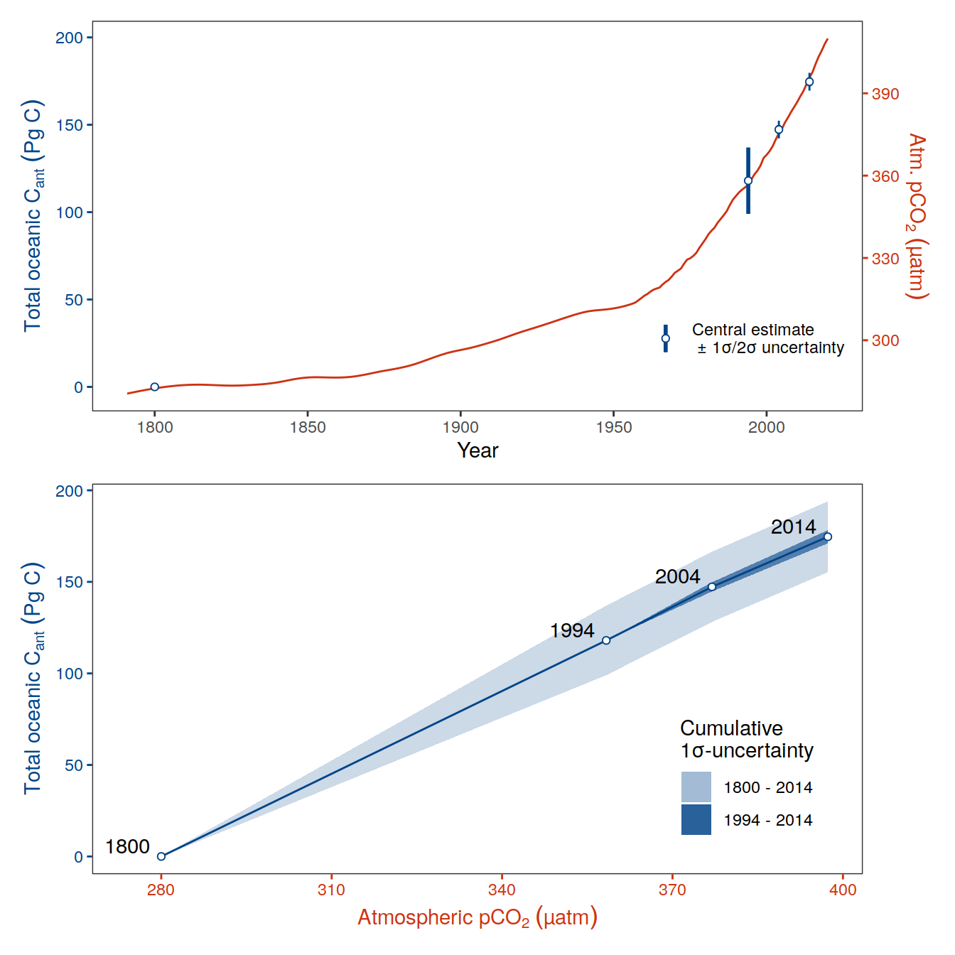
| Version | Author | Date |
|---|---|---|
| 2cca4eb | jens-daniel-mueller | 2023-01-10 |
| 0f2c9d5 | jens-daniel-mueller | 2022-12-08 |
| 3a7bab0 | jens-daniel-mueller | 2022-11-28 |
| 322b1c1 | jens-daniel-mueller | 2022-11-25 |
| 491f8b1 | jens-daniel-mueller | 2022-11-25 |
| 4da4d66 | jens-daniel-mueller | 2022-11-25 |
| 534ee74 | jens-daniel-mueller | 2022-11-25 |
| e924c80 | jens-daniel-mueller | 2022-11-17 |
| ea34027 | jens-daniel-mueller | 2022-11-15 |
| 1dad51a | jens-daniel-mueller | 2022-11-15 |
| 375300e | jens-daniel-mueller | 2022-11-14 |
| 6edad9b | jens-daniel-mueller | 2022-11-11 |
| 16beb51 | jens-daniel-mueller | 2022-11-08 |
| b92657d | jens-daniel-mueller | 2022-11-08 |
| 7275091 | jens-daniel-mueller | 2022-11-05 |
| 99610ed | jens-daniel-mueller | 2022-11-01 |
| 7060801 | jens-daniel-mueller | 2022-10-31 |
| ecb84c1 | jens-daniel-mueller | 2022-10-30 |
| 2345935 | jens-daniel-mueller | 2022-10-29 |
| 91052ae | jens-daniel-mueller | 2022-10-20 |
| b1f7ab3 | jens-daniel-mueller | 2022-07-18 |
| d2ae54c | jens-daniel-mueller | 2022-07-18 |
| 2695085 | jens-daniel-mueller | 2022-07-17 |
| 535196a | jens-daniel-mueller | 2022-07-17 |
| afb27ad | jens-daniel-mueller | 2022-07-15 |
| b492b46 | jens-daniel-mueller | 2022-07-15 |
| bd24a0f | jens-daniel-mueller | 2022-07-15 |
| 17cd1d1 | jens-daniel-mueller | 2022-07-13 |
| 8fb595c | jens-daniel-mueller | 2022-07-12 |
| 003b161 | jens-daniel-mueller | 2022-07-12 |
| 8ab4a87 | jens-daniel-mueller | 2022-06-29 |
| 7629c78 | jens-daniel-mueller | 2022-06-29 |
| f6786c8 | jens-daniel-mueller | 2022-06-29 |
| 0825298 | jens-daniel-mueller | 2022-06-28 |
| 87e9eb8 | jens-daniel-mueller | 2022-06-27 |
| b52b159 | jens-daniel-mueller | 2022-06-27 |
| 1d73ec9 | jens-daniel-mueller | 2022-05-16 |
| 2ca0109 | jens-daniel-mueller | 2022-05-02 |
| b018a9a | jens-daniel-mueller | 2022-04-29 |
| e09320d | jens-daniel-mueller | 2022-04-12 |
| 8dca96a | jens-daniel-mueller | 2022-04-12 |
| 209c9b6 | jens-daniel-mueller | 2022-04-10 |
| acad2e2 | jens-daniel-mueller | 2022-04-09 |
| 3d81135 | jens-daniel-mueller | 2022-04-07 |
| a74e341 | jens-daniel-mueller | 2022-04-04 |
| 5a6be34 | jens-daniel-mueller | 2022-03-22 |
| bd9e11d | jens-daniel-mueller | 2022-03-22 |
| 2501978 | jens-daniel-mueller | 2022-03-21 |
| 251c7cf | jens-daniel-mueller | 2022-02-17 |
| 565224d | jens-daniel-mueller | 2022-02-17 |
| 2116dd3 | jens-daniel-mueller | 2022-02-09 |
ggsave(path = here::here("output/presentation"),
filename = "Fig_dcant_budget_global_vs_atm_pCO2.png",
height = 6,
width = 7)
p_tcant_year_trans / p_tcant_atm_co2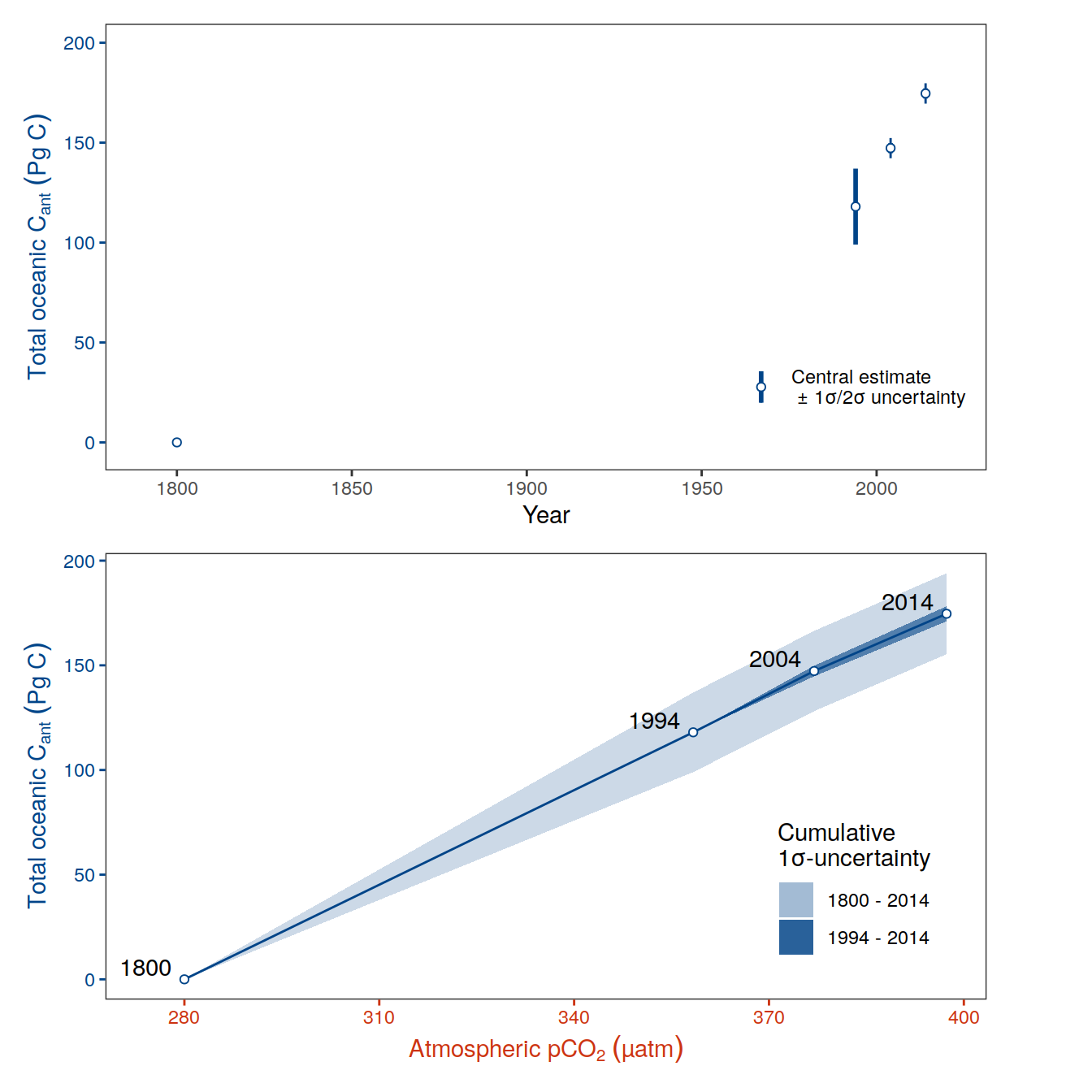
| Version | Author | Date |
|---|---|---|
| fdf5f22 | jens-daniel-mueller | 2023-01-11 |
| 2cca4eb | jens-daniel-mueller | 2023-01-10 |
| 3a7bab0 | jens-daniel-mueller | 2022-11-28 |
| 322b1c1 | jens-daniel-mueller | 2022-11-25 |
| 491f8b1 | jens-daniel-mueller | 2022-11-25 |
| 4da4d66 | jens-daniel-mueller | 2022-11-25 |
| 534ee74 | jens-daniel-mueller | 2022-11-25 |
| e924c80 | jens-daniel-mueller | 2022-11-17 |
| ea34027 | jens-daniel-mueller | 2022-11-15 |
| 1dad51a | jens-daniel-mueller | 2022-11-15 |
| 375300e | jens-daniel-mueller | 2022-11-14 |
| 6edad9b | jens-daniel-mueller | 2022-11-11 |
| 16beb51 | jens-daniel-mueller | 2022-11-08 |
| b92657d | jens-daniel-mueller | 2022-11-08 |
| 7275091 | jens-daniel-mueller | 2022-11-05 |
| 99610ed | jens-daniel-mueller | 2022-11-01 |
| 7060801 | jens-daniel-mueller | 2022-10-31 |
| ecb84c1 | jens-daniel-mueller | 2022-10-30 |
| 2345935 | jens-daniel-mueller | 2022-10-29 |
| 91052ae | jens-daniel-mueller | 2022-10-20 |
ggsave(path = here::here("output/presentation"),
filename = "Fig_dcant_budget_global_vs_atm_pCO2_trans.png",
height = 6,
width = 7)tcant_ts %>%
mutate(beta = dcant_mean / (pCO2-lag(pCO2)))# A tibble: 4 × 8
year dcant_mean dcant_sd dcant_sd_int pCO2 tcant tcant_sd beta
<dbl> <dbl> <dbl> <dbl> <dbl> <dbl> <dbl> <dbl>
1 1800 0 NA NA 280 0 0 NA
2 1994 118 0 19 358. 118 19 1.51
3 2004 29.3 2.53 2.53 377. 147. 19.2 1.57
4 2014 27.3 3.59 2.55 397. 175. 19.3 1.3416.2 incl fluxes
Ocean_Sink <- Ocean_Sink %>%
filter(product != "Watson")Ocean_Sink %>%
filter(year >= 2010, year <= 2019) %>%
group_by(type) %>%
summarise(GtC_yr_mean = mean(GtC_yr)) %>%
ungroup()# A tibble: 2 × 2
type GtC_yr_mean
<chr> <dbl>
1 data_products 3.02
2 models 2.46Ocean_Sink_cum_1994 <-
Ocean_Sink %>%
filter(year >= 1994, year <= 2007) %>%
mutate(fgco2_glob = if_else(year == 1994, 0, GtC_yr),
fgco2_glob = fgco2_glob) %>%
arrange(year) %>%
group_by(product, type) %>%
mutate(fgco2_glob_cum = cumsum(fgco2_glob)) %>%
ungroup()
Ocean_Sink_cum_1994 <-
left_join(Ocean_Sink_cum_1994,
co2_atm)
Ocean_Sink_cum_1994 %>%
group_split(type) %>%
map(
~ ggplot(data = .x, aes(pCO2, fgco2_glob_cum, col = product)) +
geom_line() +
geom_point(shape = 21, fill = "white") +
theme(legend.position = "bottom") +
facet_grid(. ~ type)
)[[1]]
[[2]]
Ocean_Sink_cum_1994 <- Ocean_Sink_cum_1994 %>%
mutate(fgco2_glob_cum_total = fgco2_glob_cum + 118) %>%
select(year, pCO2, product, fgco2_glob_cum, fgco2_glob_cum_total, type)
Ocean_Sink_cum_1994 <- Ocean_Sink_cum_1994 %>%
mutate(type = case_when(
type == "data_products" ~ "Observation-based\nsurface flux\nproducts",
TRUE ~ "Global Ocean\nBiogeochemical Models\n(GOBM)"
))
Ocean_Sink_cum_1994 %>%
filter(year == 2007) %>%
group_by(type) %>%
summarise(dcant_sd = sd(fgco2_glob_cum)*sd_factor) %>%
ungroup()# A tibble: 2 × 2
type dcant_sd
<chr> <dbl>
1 "Global Ocean\nBiogeochemical Models\n(GOBM)" 6.99
2 "Observation-based\nsurface flux\nproducts" 6.66Ocean_Sink_cum_1994 <-
Ocean_Sink %>%
filter(year >= 1994, year <= 2014) %>%
mutate(fgco2_glob = if_else(year == 1994, 0, GtC_yr),
fgco2_glob = fgco2_glob) %>%
arrange(year) %>%
group_by(product, type) %>%
mutate(fgco2_glob_cum = cumsum(fgco2_glob)) %>%
ungroup()
Ocean_Sink_cum_1994 <-
left_join(Ocean_Sink_cum_1994,
co2_atm)
Ocean_Sink_cum_1994 %>%
group_split(type) %>%
map(
~ ggplot(data = .x, aes(pCO2, fgco2_glob_cum, col = product)) +
geom_line() +
geom_point(shape = 21, fill = "white") +
theme(legend.position = "bottom") +
facet_grid(. ~ type)
)[[1]]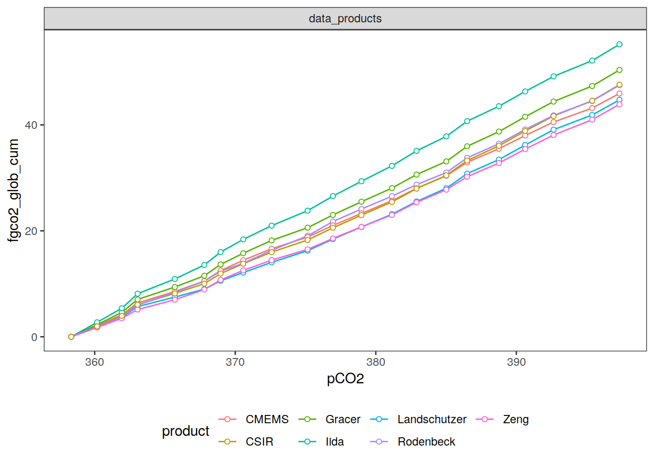
[[2]]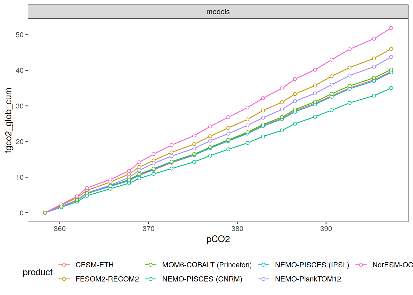
Ocean_Sink_cum_1994 <- Ocean_Sink_cum_1994 %>%
mutate(fgco2_glob_cum_total = fgco2_glob_cum + 118) %>%
select(year, pCO2, product, fgco2_glob_cum, fgco2_glob_cum_total, type)
Ocean_Sink_cum_1994 <- Ocean_Sink_cum_1994 %>%
mutate(type = case_when(
type == "data_products" ~ "Observation-based\nsurface flux\nproducts",
TRUE ~ "Global Ocean\nBiogeochemical Models\n(GOBM)"
))tcant_2004 <- tcant_ts %>%
filter(year == 2004) %>%
pull(tcant)
Ocean_Sink_cum_2004 <-
Ocean_Sink %>%
filter(year >= 2004, year <= 2014) %>%
mutate(fgco2_glob = if_else(year == 2004, 0, GtC_yr)) %>%
arrange(year) %>%
group_by(product, type) %>%
mutate(fgco2_glob_cum = cumsum(fgco2_glob)) %>%
ungroup()
Ocean_Sink_cum_2004 <-
left_join(Ocean_Sink_cum_2004,
co2_atm)
Ocean_Sink_cum_2004 %>%
group_split(type) %>%
map(
~ ggplot(data = .x, aes(pCO2, fgco2_glob_cum, col = product)) +
geom_line() +
geom_point(shape = 21, fill = "white") +
theme(legend.position = "bottom") +
facet_grid(. ~ type)
)[[1]]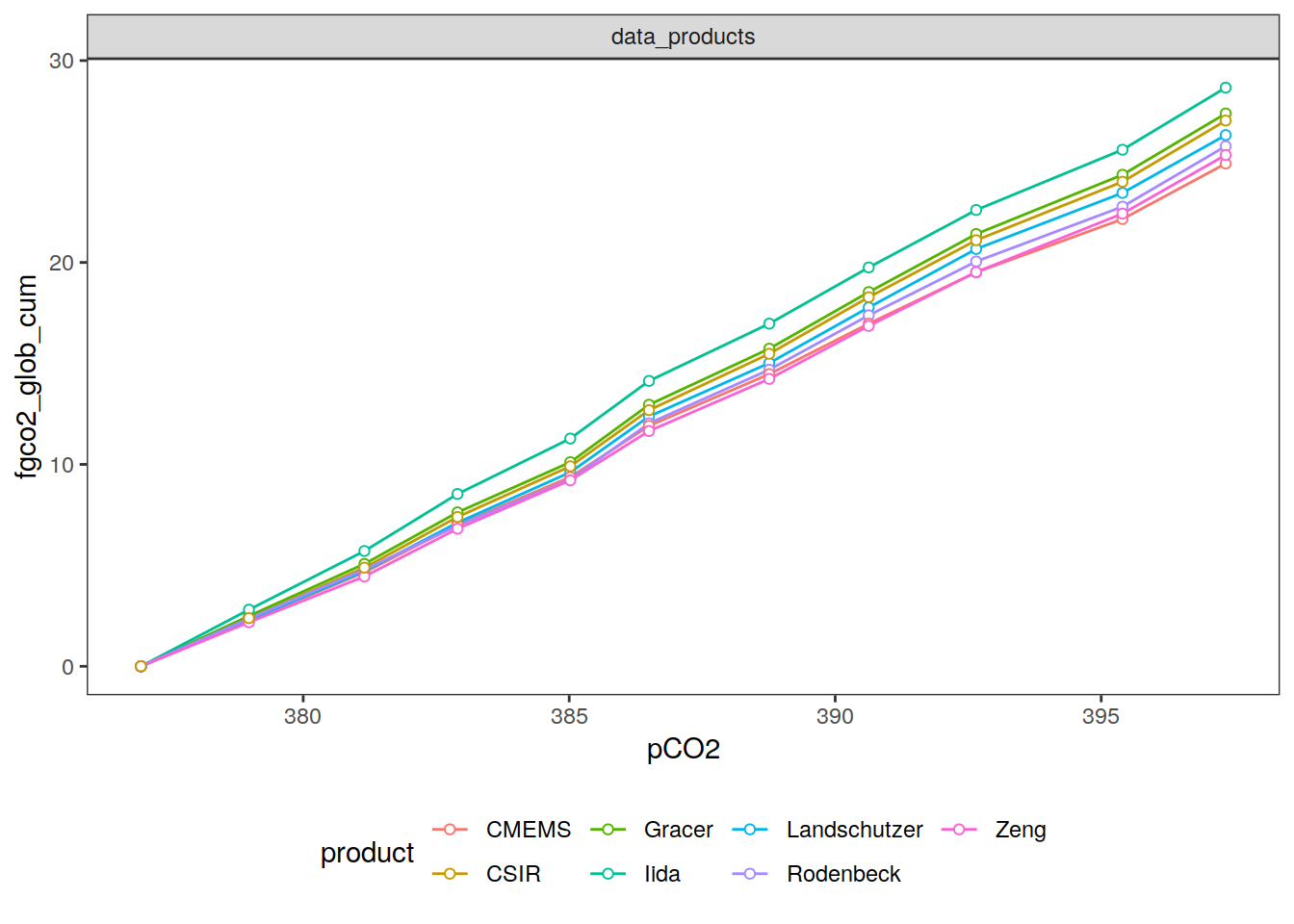
[[2]]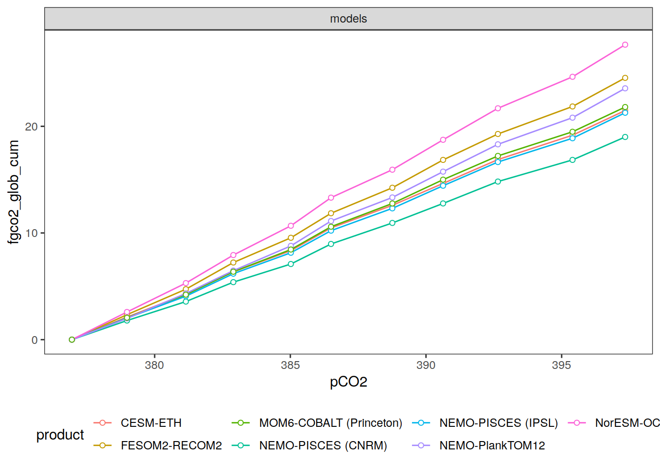
Ocean_Sink_cum_2004 <- Ocean_Sink_cum_2004 %>%
mutate(fgco2_glob_cum_total = fgco2_glob_cum + tcant_2004) %>%
select(year, pCO2, product, fgco2_glob_cum, fgco2_glob_cum_total, type)
Ocean_Sink_cum_2004 <- Ocean_Sink_cum_2004 %>%
mutate(type = case_when(
type == "data_products" ~ "Observation-based\nsurface flux\nproducts",
TRUE ~ "Global Ocean\nBiogeochemical Models\n(GOBM)"
))tcant_ts_zoom <- tcant_ts %>%
filter(year != 1800)
tcant_ts_zoom <-
tcant_ts_zoom %>%
mutate(tcant = tcant - 118)
tcant_min = tcant_ts_zoom %>% pull(tcant) %>% min()
tcant_max =
tcant_ts_zoom %>% pull(tcant) %>% max() +
tcant_ts_zoom %>% pull(dcant_sd) %>% max()*2
Ocean_Sink_cum_1994 <-
Ocean_Sink_cum_1994 %>%
mutate(fgco2_glob_cum_total = fgco2_glob_cum_total - 118)
Ocean_Sink_cum_2004 <-
Ocean_Sink_cum_2004 %>%
mutate(fgco2_glob_cum_total = fgco2_glob_cum_total - 118)
p_tcant_ts_zoom <-
tcant_ts_zoom %>%
ggplot(aes(pCO2, tcant)) +
geom_ribbon(
aes(ymin = tcant - dcant_sd*2,
ymax = tcant + dcant_sd*2),
alpha = 0.2,
fill = tcant_col
) +
geom_ribbon(
aes(
ymin = tcant - dcant_sd,
ymax = tcant + dcant_sd
),
alpha = 0.3,
fill = tcant_col
) +
geom_line(data = Ocean_Sink_cum_1994,
aes(pCO2, fgco2_glob_cum_total, group = product, col = type)) +
geom_point(
data = Ocean_Sink_cum_1994,
aes(pCO2, fgco2_glob_cum_total, group = product, col = type),
size = 0.3
) +
geom_point(
data = Ocean_Sink_cum_1994 %>% filter(year %in% c(2004, 2014)),
aes(
pCO2,
fgco2_glob_cum_total,
col = type
),
fill = "white",
shape = 21
) +
geom_line(aes(col = "eMLR(C*)")) +
geom_point(aes(col = "eMLR(C*)"),
shape = 21,
fill = "white") +
geom_text(aes(label = year), nudge_x = -2, nudge_y = 3) +
scale_color_highcontrast(name = "Data source") +
scale_fill_highcontrast(name = "Data source") +
scale_y_continuous(limits = c(tcant_min, tcant_max)) +
labs(x = expression(Atmospheric ~ pCO[2] ~ (µatm)),
y = expression(Cumulative ~ ocean ~ carbon ~ storage ~ since ~ 1994 ~ (Pg~C))) +
guides(colour = guide_legend(order = 1),
fill = "none") +
theme_classic() +
theme(
legend.background = element_rect(fill = "transparent"),
legend.position = c(0.25, 0.83),
legend.title = element_blank(),
legend.box.just = "top",
legend.box = "horizontal",
legend.key.size = unit(2.5, 'lines'),
panel.grid.major.y = element_line(colour = "black",
size = 0.1)
)
p_tcant_ts_zoom
| Version | Author | Date |
|---|---|---|
| 322b1c1 | jens-daniel-mueller | 2022-11-25 |
| 491f8b1 | jens-daniel-mueller | 2022-11-25 |
| 4da4d66 | jens-daniel-mueller | 2022-11-25 |
| 534ee74 | jens-daniel-mueller | 2022-11-25 |
| e924c80 | jens-daniel-mueller | 2022-11-17 |
| 8e1702d | jens-daniel-mueller | 2022-11-16 |
| ea34027 | jens-daniel-mueller | 2022-11-15 |
| 8ac0da0 | jens-daniel-mueller | 2022-11-15 |
| 1dad51a | jens-daniel-mueller | 2022-11-15 |
| 375300e | jens-daniel-mueller | 2022-11-14 |
| ebc85e2 | jens-daniel-mueller | 2022-11-14 |
| 6edad9b | jens-daniel-mueller | 2022-11-11 |
| 16beb51 | jens-daniel-mueller | 2022-11-08 |
| b92657d | jens-daniel-mueller | 2022-11-08 |
| 7275091 | jens-daniel-mueller | 2022-11-05 |
| 99610ed | jens-daniel-mueller | 2022-11-01 |
| 7060801 | jens-daniel-mueller | 2022-10-31 |
| ecb84c1 | jens-daniel-mueller | 2022-10-30 |
| 2345935 | jens-daniel-mueller | 2022-10-29 |
| 91052ae | jens-daniel-mueller | 2022-10-20 |
| 8105380 | jens-daniel-mueller | 2022-10-07 |
| f68fcfa | jens-daniel-mueller | 2022-07-26 |
| f2615fb | jens-daniel-mueller | 2022-07-26 |
| 4af29f9 | jens-daniel-mueller | 2022-07-24 |
| b18b250 | jens-daniel-mueller | 2022-07-20 |
| a80b59b | jens-daniel-mueller | 2022-07-20 |
| fea41c1 | jens-daniel-mueller | 2022-07-20 |
| d803308 | jens-daniel-mueller | 2022-07-19 |
| b1f7ab3 | jens-daniel-mueller | 2022-07-18 |
| d2ae54c | jens-daniel-mueller | 2022-07-18 |
| 2695085 | jens-daniel-mueller | 2022-07-17 |
| 535196a | jens-daniel-mueller | 2022-07-17 |
| afb27ad | jens-daniel-mueller | 2022-07-15 |
| b492b46 | jens-daniel-mueller | 2022-07-15 |
| bd24a0f | jens-daniel-mueller | 2022-07-15 |
| 17cd1d1 | jens-daniel-mueller | 2022-07-13 |
| 8fb595c | jens-daniel-mueller | 2022-07-12 |
| 003b161 | jens-daniel-mueller | 2022-07-12 |
| 8ab4a87 | jens-daniel-mueller | 2022-06-29 |
| 7629c78 | jens-daniel-mueller | 2022-06-29 |
| f6786c8 | jens-daniel-mueller | 2022-06-29 |
| 9393c07 | jens-daniel-mueller | 2022-06-28 |
| 0825298 | jens-daniel-mueller | 2022-06-28 |
| fb59a6f | jens-daniel-mueller | 2022-06-27 |
| 3c1100c | jens-daniel-mueller | 2022-05-16 |
| 2ca0109 | jens-daniel-mueller | 2022-05-02 |
| b018a9a | jens-daniel-mueller | 2022-04-29 |
| e09320d | jens-daniel-mueller | 2022-04-12 |
| 8dca96a | jens-daniel-mueller | 2022-04-12 |
| 209c9b6 | jens-daniel-mueller | 2022-04-10 |
| acad2e2 | jens-daniel-mueller | 2022-04-09 |
| 3d81135 | jens-daniel-mueller | 2022-04-07 |
| a74e341 | jens-daniel-mueller | 2022-04-04 |
| bd9e11d | jens-daniel-mueller | 2022-03-22 |
| 2501978 | jens-daniel-mueller | 2022-03-21 |
| c3a6238 | jens-daniel-mueller | 2022-03-08 |
| 094bfa0 | jens-daniel-mueller | 2022-02-18 |
| ba2d62e | jens-daniel-mueller | 2022-02-17 |
| 192504c | jens-daniel-mueller | 2022-02-17 |
| d2191ad | jens-daniel-mueller | 2022-02-04 |
| 4c5b079 | jens-daniel-mueller | 2022-02-03 |
| 4077397 | jens-daniel-mueller | 2022-02-03 |
dcant_type_box <-
bind_rows(
dcant_budget_basin_MLR_all_ensemble %>%
filter(
data_source == "obs",
basin == "Global",
!(Version_ID %in% Version_IDs),
MLR_basins == unique(params_local_all$MLR_basins) |
Version_ID_group == unique(params_local_all$Version_ID_group)
) %>%
select(period, dcant) %>%
mutate(type = "eMLR(C*)",
dcant = dcant,
dcant = if_else(period == "2004 - 2014",
dcant + tcant_2004 - 118,
dcant)),
Ocean_Sink_cum_1994 %>%
filter(year %in% c(2004, 2014)) %>%
mutate(period = if_else(year == 2004,
"1994 - 2004",
"1994 - 2014")) %>%
select(period, dcant = fgco2_glob_cum_total, type),
Ocean_Sink_cum_2004 %>%
filter(year %in% c(2014)) %>%
mutate(period = if_else(year == 2014,
"2004 - 2014",
"other")) %>%
select(period, dcant = fgco2_glob_cum_total, type)
)
dcant_type_box_stat <- dcant_type_box %>%
group_by(period, type) %>%
summarise(dcant_mean = mean(dcant),
dcant_sd = sd(dcant)) %>%
ungroup()
dcant_type_box_stat <-
left_join(
dcant_type_box_stat,
dcant_budget_basin_MLR_all_uncertainty %>%
filter(data_source == "obs",
basin == "Global") %>%
mutate(
std_case = if_else(period == "2004 - 2014",
std_case + tcant_2004 - 118,
std_case)
) %>%
select(period, std_case, sd)
)
dcant_type_box_stat <- dcant_type_box_stat %>%
mutate(dcant_mean = if_else(type == "eMLR(C*)",
std_case,
dcant_mean)) %>%
mutate(dcant_sd = if_else(type == "eMLR(C*)",
sd,
dcant_sd)) %>%
select(-c(std_case, sd))
p_tcant_box <-
dcant_type_box %>%
filter(period == "1994 - 2014") %>%
ggplot(aes(period, dcant)) +
geom_crossbar(
data = dcant_type_box_stat %>%
filter(period == "1994 - 2014"),
position = position_dodge(width = 1),
aes(
x = period,
y = dcant_mean,
ymin = dcant_mean - dcant_sd*2,
ymax = dcant_mean + dcant_sd*2,
col = type,
fill = type
), width = 0.7, alpha = 0.2
) +
geom_crossbar(
data = dcant_type_box_stat %>%
filter(period == "1994 - 2014"),
position = position_dodge(width = 1),
aes(
x = period,
y = dcant_mean,
ymin = dcant_mean - dcant_sd,
ymax = dcant_mean + dcant_sd,
col = type,
fill = type
), width = 0.7, alpha = 0.4
) +
geom_point(aes(fill = type),
position = position_jitterdodge(
dodge.width = 1,
jitter.width = 0.1),
shape = 21,
alpha = 0.5) +
scale_fill_highcontrast(
name = "Data source",
guide = "none"
) +
scale_color_highcontrast(
name = "Data source",
guide = "none"
) +
scale_y_continuous(limits = c(tcant_min, tcant_max)) +
labs(x = "20yr period") +
theme_classic() +
theme(
axis.line.y.left = element_blank(),
axis.text.y = element_blank(),
axis.ticks.y = element_blank(),
axis.title.y = element_blank(),
panel.grid.major.y = element_line(colour = "black",
size = 0.1)
)
name_sec_axis <- expression(
atop(Cumulative ~ ocean ~ carbon ~ storage,
since ~ 2004 ~ (Pg ~ C)))
p_tcant_box_10 <-
dcant_type_box %>%
filter(period != "1994 - 2014") %>%
ggplot(aes(period, dcant)) +
geom_crossbar(
data = dcant_type_box_stat %>%
filter(period != "1994 - 2014"),
position = position_dodge(width = 1),
aes(
x = period,
y = dcant_mean,
ymin = dcant_mean - dcant_sd*2,
ymax = dcant_mean + dcant_sd*2,
col = type,
fill = type
),
width = 0.7,
alpha = 0.2
) +
geom_crossbar(
data = dcant_type_box_stat %>%
filter(period != "1994 - 2014"),
position = position_dodge(width = 1),
aes(
x = period,
y = dcant_mean,
ymin = dcant_mean - dcant_sd,
ymax = dcant_mean + dcant_sd,
col = type,
fill = type
),
width = 0.7,
alpha = 0.4
) +
geom_point(
aes(fill = type),
position = position_jitterdodge(dodge.width = 1,
jitter.width = 0.1),
shape = 21,
alpha = 0.5
) +
geom_point(
data = dcant_type_box_stat %>%
filter(period != "1994 - 2014"),
position = position_dodge(width = 1),
aes(x = period,
y = dcant_mean,
col = type),
fill = "white",
shape = 21,
size = 2
) +
scale_fill_highcontrast(name = "Data source",
guide = "none") +
scale_color_highcontrast(name = "Data source",
guide = "none") +
scale_y_continuous(
limits = c(tcant_min, tcant_max),
sec.axis = sec_axis(
~ . - (tcant_2004 - 118),
name = name_sec_axis,
guide = guide_axis_truncated(trunc_lower = tcant_2004 - 118,
trunc_upper = tcant_2004 - 118 + 35),
breaks = seq(0, 30, 10)
)
)+
labs(x = "Decades")+
theme_classic() +
# guides(y.right = "axis_truncated") +
theme(
axis.line.y.left = element_blank(),
axis.text.y.left = element_blank(),
axis.ticks.y.left = element_blank(),
axis.title.y.left = element_blank(),
panel.grid.major.y = element_line(colour = "black",
size = 0.1)
)
p_tcant_box_10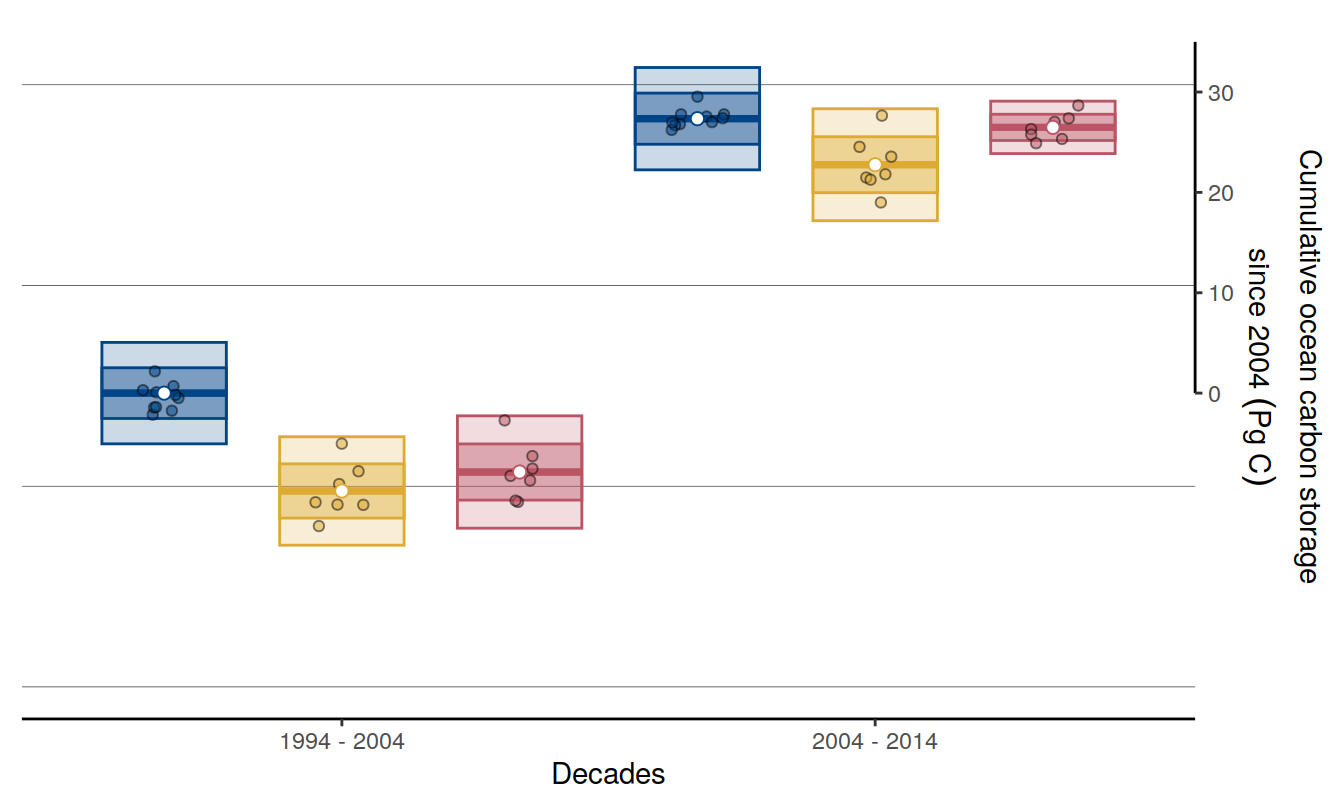
| Version | Author | Date |
|---|---|---|
| 2cca4eb | jens-daniel-mueller | 2023-01-10 |
| b9d5a73 | jens-daniel-mueller | 2022-12-15 |
| 0f2c9d5 | jens-daniel-mueller | 2022-12-08 |
| 322b1c1 | jens-daniel-mueller | 2022-11-25 |
| 491f8b1 | jens-daniel-mueller | 2022-11-25 |
| 4da4d66 | jens-daniel-mueller | 2022-11-25 |
| 534ee74 | jens-daniel-mueller | 2022-11-25 |
| e924c80 | jens-daniel-mueller | 2022-11-17 |
| 8e1702d | jens-daniel-mueller | 2022-11-16 |
| ea34027 | jens-daniel-mueller | 2022-11-15 |
| 8ac0da0 | jens-daniel-mueller | 2022-11-15 |
| 1dad51a | jens-daniel-mueller | 2022-11-15 |
| 375300e | jens-daniel-mueller | 2022-11-14 |
| ebc85e2 | jens-daniel-mueller | 2022-11-14 |
| 6edad9b | jens-daniel-mueller | 2022-11-11 |
| 16beb51 | jens-daniel-mueller | 2022-11-08 |
| b92657d | jens-daniel-mueller | 2022-11-08 |
| 7275091 | jens-daniel-mueller | 2022-11-05 |
| 99610ed | jens-daniel-mueller | 2022-11-01 |
| 7060801 | jens-daniel-mueller | 2022-10-31 |
| ecb84c1 | jens-daniel-mueller | 2022-10-30 |
| 2345935 | jens-daniel-mueller | 2022-10-29 |
| 0b40366 | jens-daniel-mueller | 2022-10-26 |
| 91052ae | jens-daniel-mueller | 2022-10-20 |
| 77e6a80 | jens-daniel-mueller | 2022-09-08 |
| 051b911 | jens-daniel-mueller | 2022-09-07 |
| 75bd58c | jens-daniel-mueller | 2022-09-07 |
| 1c6de0d | jens-daniel-mueller | 2022-09-07 |
| 78dbb27 | jens-daniel-mueller | 2022-08-11 |
| 302d289 | jens-daniel-mueller | 2022-08-11 |
| 318fefe | jens-daniel-mueller | 2022-08-11 |
| 5b77c4f | jens-daniel-mueller | 2022-08-10 |
| 9c3be27 | jens-daniel-mueller | 2022-08-09 |
| a691b29 | jens-daniel-mueller | 2022-08-09 |
| 910f96e | jens-daniel-mueller | 2022-08-08 |
| f68fcfa | jens-daniel-mueller | 2022-07-26 |
| f2615fb | jens-daniel-mueller | 2022-07-26 |
| 4af29f9 | jens-daniel-mueller | 2022-07-24 |
| b18b250 | jens-daniel-mueller | 2022-07-20 |
| a80b59b | jens-daniel-mueller | 2022-07-20 |
| fea41c1 | jens-daniel-mueller | 2022-07-20 |
| d803308 | jens-daniel-mueller | 2022-07-19 |
| b1f7ab3 | jens-daniel-mueller | 2022-07-18 |
| d2ae54c | jens-daniel-mueller | 2022-07-18 |
| 2695085 | jens-daniel-mueller | 2022-07-17 |
| 535196a | jens-daniel-mueller | 2022-07-17 |
| d20faeb | jens-daniel-mueller | 2022-07-17 |
| afb27ad | jens-daniel-mueller | 2022-07-15 |
| b492b46 | jens-daniel-mueller | 2022-07-15 |
| bd24a0f | jens-daniel-mueller | 2022-07-15 |
| 17cd1d1 | jens-daniel-mueller | 2022-07-13 |
| 26e9496 | jens-daniel-mueller | 2022-07-12 |
| 8fb595c | jens-daniel-mueller | 2022-07-12 |
| 003b161 | jens-daniel-mueller | 2022-07-12 |
| 8ab4a87 | jens-daniel-mueller | 2022-06-29 |
| 7629c78 | jens-daniel-mueller | 2022-06-29 |
| f6786c8 | jens-daniel-mueller | 2022-06-29 |
| 9393c07 | jens-daniel-mueller | 2022-06-28 |
| 0825298 | jens-daniel-mueller | 2022-06-28 |
p_tcant_ts_zoom + p_tcant_box + p_tcant_box_10 +
plot_layout(ncol = 3, widths = c(6,1,1.8)) +
plot_annotation(tag_levels = 'A')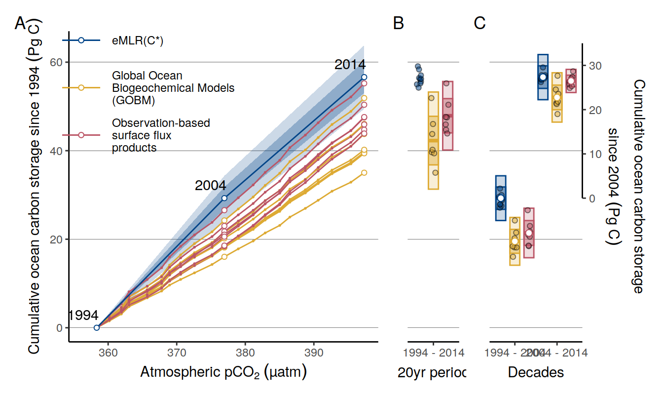
| Version | Author | Date |
|---|---|---|
| 2cca4eb | jens-daniel-mueller | 2023-01-10 |
| b9d5a73 | jens-daniel-mueller | 2022-12-15 |
| 0f2c9d5 | jens-daniel-mueller | 2022-12-08 |
| 322b1c1 | jens-daniel-mueller | 2022-11-25 |
| 491f8b1 | jens-daniel-mueller | 2022-11-25 |
| 4da4d66 | jens-daniel-mueller | 2022-11-25 |
| 534ee74 | jens-daniel-mueller | 2022-11-25 |
| e924c80 | jens-daniel-mueller | 2022-11-17 |
| 8e1702d | jens-daniel-mueller | 2022-11-16 |
| ea34027 | jens-daniel-mueller | 2022-11-15 |
| 8ac0da0 | jens-daniel-mueller | 2022-11-15 |
| 1dad51a | jens-daniel-mueller | 2022-11-15 |
| 375300e | jens-daniel-mueller | 2022-11-14 |
| ebc85e2 | jens-daniel-mueller | 2022-11-14 |
| 6edad9b | jens-daniel-mueller | 2022-11-11 |
| 16beb51 | jens-daniel-mueller | 2022-11-08 |
| b92657d | jens-daniel-mueller | 2022-11-08 |
| 7275091 | jens-daniel-mueller | 2022-11-05 |
| 99610ed | jens-daniel-mueller | 2022-11-01 |
| 7060801 | jens-daniel-mueller | 2022-10-31 |
| ecb84c1 | jens-daniel-mueller | 2022-10-30 |
| 2345935 | jens-daniel-mueller | 2022-10-29 |
| 0b40366 | jens-daniel-mueller | 2022-10-26 |
| 91052ae | jens-daniel-mueller | 2022-10-20 |
# ggsave(path = here::here("output/publication"),
# filename = "Fig_dcant_inventory_global_vs_GCB_ocean_sink.png",
# height = 6,
# width = 9)
p_tcant_ts_zoom + p_tcant_box_10 +
plot_layout(ncol = 2, widths = c(6,1.8))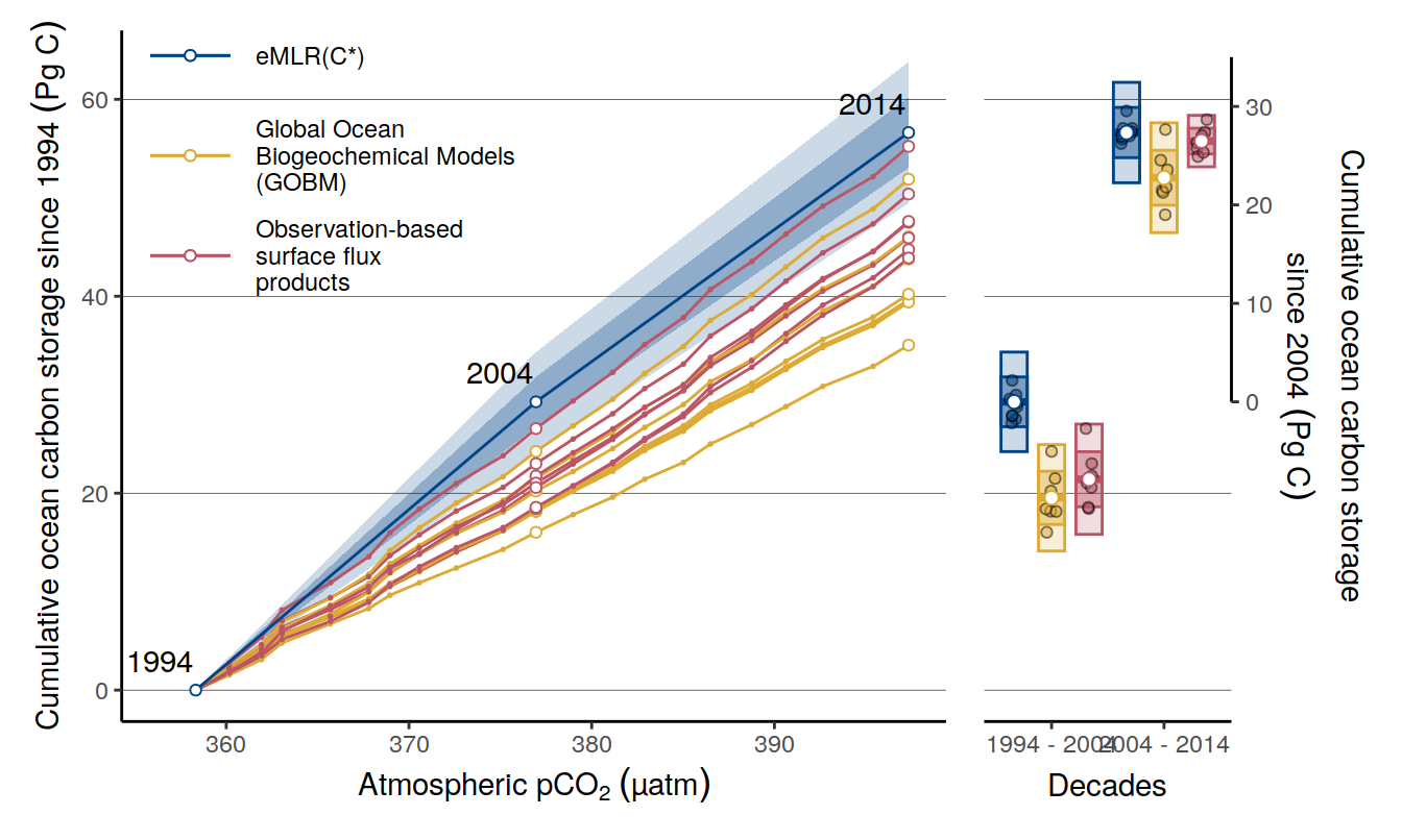
| Version | Author | Date |
|---|---|---|
| 2cca4eb | jens-daniel-mueller | 2023-01-10 |
ggsave(path = here::here("output/presentation"),
filename = "Fig_dcant_budget_global_vs_GCB_ocean_sink.png",
height = 6,
width = 9)
dcant_type_significance <- dcant_type_box_stat %>%
mutate(dcant_mean = dcant_mean,
dcant_mean = if_else(period == "2004 - 2014",
dcant_mean - (tcant_2004 - 118),
dcant_mean)) %>%
group_by(period) %>%
mutate(
dcant_diff = dcant_mean - first(dcant_mean),
dcant_diff_rel = 100 * dcant_diff / first(dcant_mean),
dcant_diff_sd = sqrt(dcant_sd ^ 2 + first(dcant_sd) ^ 2),
dcant_diff_sd_comparison = abs(dcant_diff_sd) - abs(dcant_diff)
) %>%
ungroup()
dcant_type_significance %>%
drop_na() %>%
kable() %>%
kable_styling() %>%
scroll_box(height = "300px")| period | type | dcant_mean | dcant_sd | dcant_diff | dcant_diff_rel | dcant_diff_sd | dcant_diff_sd_comparison |
|---|---|---|---|---|---|---|---|
| 1994 - 2004 | eMLR(C*) | 29.27668 | 2.527296 | 0.0000000 | 0.000000 | 3.574136 | 3.5741362 |
| 1994 - 2004 | Global Ocean Biogeochemical Models (GOBM) | 19.52578 | 2.701502 | -9.7508981 | -33.306028 | 3.699370 | -6.0515281 |
| 1994 - 2004 | Observation-based surface flux products | 21.41458 | 2.798867 | -7.8620944 | -26.854464 | 3.771058 | -4.0910360 |
| 2004 - 2014 | eMLR(C*) | 27.34720 | 2.549551 | 0.0000000 | 0.000000 | 3.605609 | 3.6056091 |
| 2004 - 2014 | Global Ocean Biogeochemical Models (GOBM) | 22.75899 | 2.788027 | -4.5882109 | -16.777624 | 3.778002 | -0.8102086 |
| 2004 - 2014 | Observation-based surface flux products | 26.48067 | 1.306376 | -0.8665297 | -3.168623 | 2.864756 | 1.9982262 |
p_tcant_box_10_dec1 <-
dcant_type_box %>%
filter(period == "1994 - 2004") %>%
ggplot(aes(period, dcant)) +
geom_crossbar(
data = dcant_type_box_stat %>%
filter(period == "1994 - 2004"),
position = position_dodge(width = 1),
aes(
x = period,
y = dcant_mean,
ymin = dcant_mean - dcant_sd*2,
ymax = dcant_mean + dcant_sd*2,
col = type,
fill = type
),
width = 0.7,
alpha = 0.2
) +
geom_crossbar(
data = dcant_type_box_stat %>%
filter(period == "1994 - 2004"),
position = position_dodge(width = 1),
aes(
x = period,
y = dcant_mean,
ymin = dcant_mean - dcant_sd,
ymax = dcant_mean + dcant_sd,
col = type,
fill = type
),
width = 0.7,
alpha = 0.4
) +
geom_point(
aes(fill = type),
position = position_jitterdodge(dodge.width = 1,
jitter.width = 0.1),
shape = 21,
alpha = 0.5
) +
geom_point(
data = dcant_type_box_stat %>%
filter(period == "1994 - 2004"),
position = position_dodge(width = 1),
aes(x = period,
y = dcant_mean,
col = type),
fill = "white",
shape = 21,
size = 2
) +
scale_fill_highcontrast(name = "Data source",
guide = "none") +
scale_color_highcontrast(name = "Data source",
guide = "none") +
scale_y_continuous(
limits = c(tcant_min, tcant_max),
breaks = seq(0,40,20)
)+
labs(x = "Decades")+
theme_classic() +
# guides(y.right = "axis_truncated") +
theme(
axis.line.y.left = element_blank(),
axis.text.y.left = element_blank(),
axis.title.x = element_blank(),
axis.ticks.y.left = element_blank(),
axis.title.y.left = element_blank(),
panel.grid.major.y = element_line(colour = "black",
size = 0.1)
)
p_tcant_box_10_dec1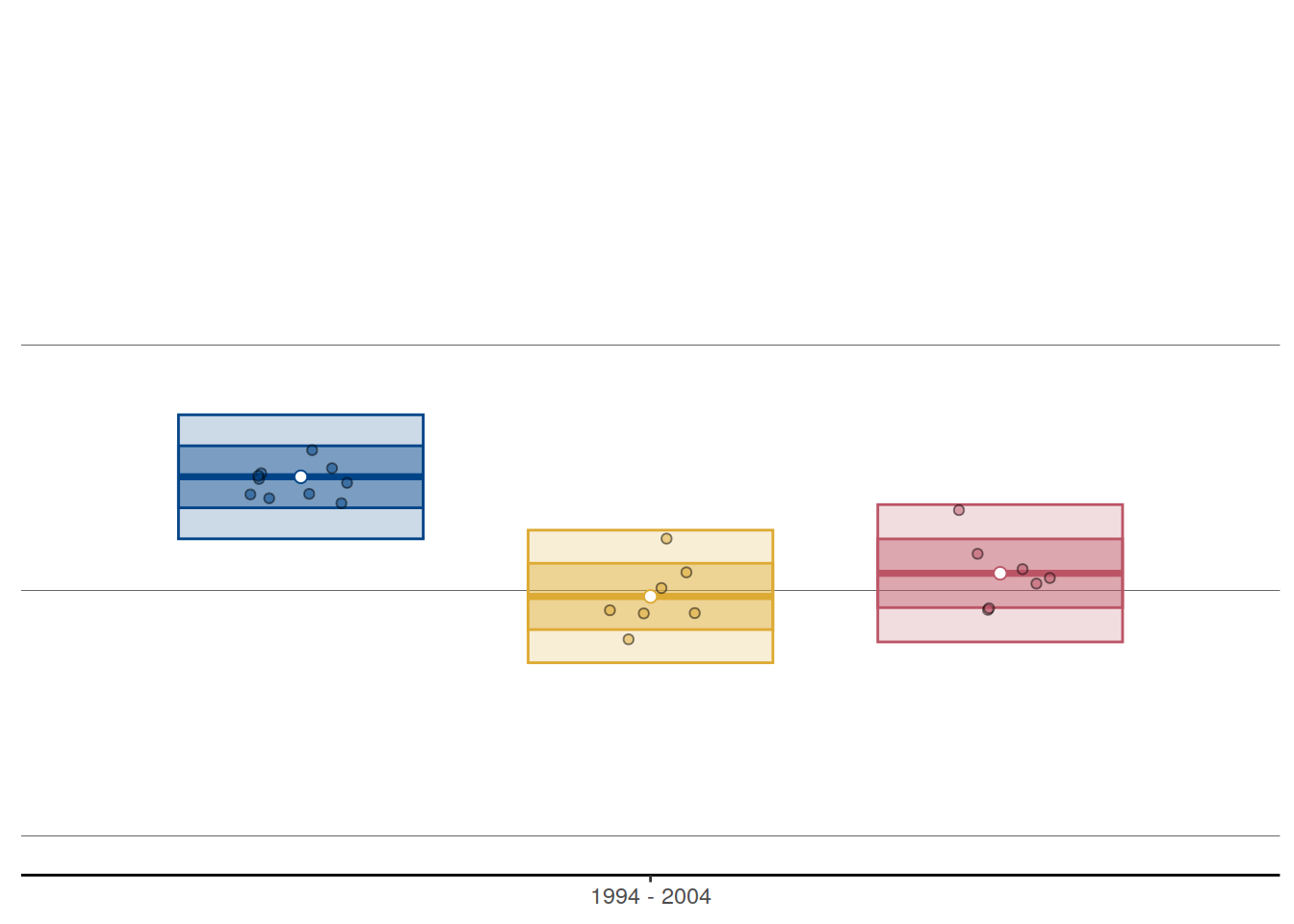
| Version | Author | Date |
|---|---|---|
| 2cca4eb | jens-daniel-mueller | 2023-01-10 |
p_tcant_box_10_dec2 <-
dcant_type_box %>%
filter(period == "2004 - 2014") %>%
ggplot(aes(period, dcant)) +
geom_crossbar(
data = dcant_type_box_stat %>%
filter(period == "2004 - 2014"),
position = position_dodge(width = 1),
aes(
x = period,
y = dcant_mean,
ymin = dcant_mean - dcant_sd*2,
ymax = dcant_mean + dcant_sd*2,
col = type,
fill = type
),
width = 0.7,
alpha = 0.2
) +
geom_crossbar(
data = dcant_type_box_stat %>%
filter(period == "2004 - 2014"),
position = position_dodge(width = 1),
aes(
x = period,
y = dcant_mean,
ymin = dcant_mean - dcant_sd,
ymax = dcant_mean + dcant_sd,
col = type,
fill = type
),
width = 0.7,
alpha = 0.4
) +
geom_point(
aes(fill = type),
position = position_jitterdodge(dodge.width = 1,
jitter.width = 0.1),
shape = 21,
alpha = 0.5
) +
geom_point(
data = dcant_type_box_stat %>%
filter(period == "2004 - 2014"),
position = position_dodge(width = 1),
aes(x = period,
y = dcant_mean,
col = type),
fill = "white",
shape = 21,
size = 2
) +
scale_fill_highcontrast(name = "Data source",
guide = "none") +
scale_color_highcontrast(name = "Data source",
guide = "none") +
scale_y_continuous(
limits = c(tcant_min, tcant_max),
breaks = seq(tcant_2004 - 118, tcant_2004 - 118 + 30, 20),
sec.axis = sec_axis(
~ . - (tcant_2004 - 118),
name = name_sec_axis,
guide = guide_axis_truncated(trunc_lower = tcant_2004 - 118,
trunc_upper = tcant_2004 - 118 + 35),
breaks = seq(0, 30, 20)
)
)+
theme_classic() +
# guides(y.right = "axis_truncated") +
theme(
axis.line.y.left = element_blank(),
axis.text.y.left = element_blank(),
axis.title.y.right = element_text(angle = 90,
hjust = 0.9),
axis.title.x = element_blank(),
axis.ticks.y.left = element_blank(),
axis.title.y.left = element_blank(),
panel.grid.major.y = element_line(colour = "black",
size = 0.1)
)
p_tcant_box_10_dec2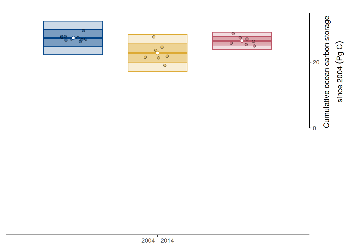
| Version | Author | Date |
|---|---|---|
| 2cca4eb | jens-daniel-mueller | 2023-01-10 |
Ocean_Sink_cum_1994_ensemble_mean <- Ocean_Sink_cum_1994 %>%
group_by(year, pCO2, type) %>%
summarise(fgco2_glob_cum_total_mean = mean(fgco2_glob_cum_total),
fgco2_glob_cum_total_sd = sd(fgco2_glob_cum_total)) %>%
ungroup()
p_tcant_ts_zoom <-
tcant_ts_zoom %>%
ggplot() +
geom_ribbon(aes(pCO2, tcant,
ymin = tcant - dcant_sd,
ymax = tcant + dcant_sd,
fill = "eMLR(C*)"),
alpha = 0.4) +
geom_ribbon(
aes(pCO2, tcant,
ymin = tcant - dcant_sd*2,
ymax = tcant + dcant_sd*2,
fill = "eMLR(C*)"),
alpha = 0.2
) +
geom_line(data = Ocean_Sink_cum_1994,
aes(pCO2, fgco2_glob_cum_total, group = product, col = type), size = 0.3) +
geom_line(data = Ocean_Sink_cum_1994_ensemble_mean,
aes(pCO2, fgco2_glob_cum_total_mean, col = type), size = 2) +
geom_point(
data = Ocean_Sink_cum_1994_ensemble_mean,
aes(pCO2, fgco2_glob_cum_total_mean, col = type), size = 1,
shape = 21,
fill = "white"
) +
geom_point(
data = Ocean_Sink_cum_1994_ensemble_mean %>% filter(year %in% c(2004, 2014)),
aes(pCO2, fgco2_glob_cum_total_mean, col = type), size = 2,
shape = 21,
fill = "white"
) +
geom_line(aes(pCO2, tcant, col = "eMLR(C*)"), size = 2) +
geom_point(aes(pCO2, tcant, col = "eMLR(C*)"), size = 2,
shape = 21,
fill = "white") +
geom_text(aes(pCO2, tcant, label = year), nudge_x = -2, nudge_y = 3) +
scale_color_highcontrast(name = "Data source") +
scale_fill_highcontrast(name = "Data source") +
scale_y_continuous(limits = c(tcant_min, tcant_max)) +
# coord_cartesian(expand = 0) +
labs(
x = expression(Atmospheric ~ pCO[2] ~ (µatm)),
y = expression(Cumulative ~ ocean ~ carbon ~ storage ~ since ~ 1994~(Pg~C))
) +
guides(colour = guide_legend(order = 1),
fill = "none") +
theme_classic() +
theme(
legend.background = element_rect(fill = "transparent"),
legend.position = c(0.25, 0.83),
legend.title = element_blank(),
legend.box.just = "top",
legend.box = "horizontal",
legend.key.size = unit(2.5, 'lines'),
panel.grid.major.y = element_line(colour = "black",
size = 0.1)
)
p_tcant_ts_zoom
| Version | Author | Date |
|---|---|---|
| 322b1c1 | jens-daniel-mueller | 2022-11-25 |
| 491f8b1 | jens-daniel-mueller | 2022-11-25 |
| 4da4d66 | jens-daniel-mueller | 2022-11-25 |
| 534ee74 | jens-daniel-mueller | 2022-11-25 |
| e924c80 | jens-daniel-mueller | 2022-11-17 |
| 8e1702d | jens-daniel-mueller | 2022-11-16 |
| ea34027 | jens-daniel-mueller | 2022-11-15 |
| 8ac0da0 | jens-daniel-mueller | 2022-11-15 |
| 1dad51a | jens-daniel-mueller | 2022-11-15 |
| 375300e | jens-daniel-mueller | 2022-11-14 |
| ebc85e2 | jens-daniel-mueller | 2022-11-14 |
| 6edad9b | jens-daniel-mueller | 2022-11-11 |
| 16beb51 | jens-daniel-mueller | 2022-11-08 |
| b92657d | jens-daniel-mueller | 2022-11-08 |
| 7275091 | jens-daniel-mueller | 2022-11-05 |
| 99610ed | jens-daniel-mueller | 2022-11-01 |
| 7060801 | jens-daniel-mueller | 2022-10-31 |
| ecb84c1 | jens-daniel-mueller | 2022-10-30 |
| 2345935 | jens-daniel-mueller | 2022-10-29 |
| 91052ae | jens-daniel-mueller | 2022-10-20 |
p_tcant_ts_zoom + p_tcant_box_10_dec1 + p_tcant_box_10_dec2 +
plot_layout(ncol = 3, widths = c(8,1,1)) +
plot_annotation(tag_levels = 'A')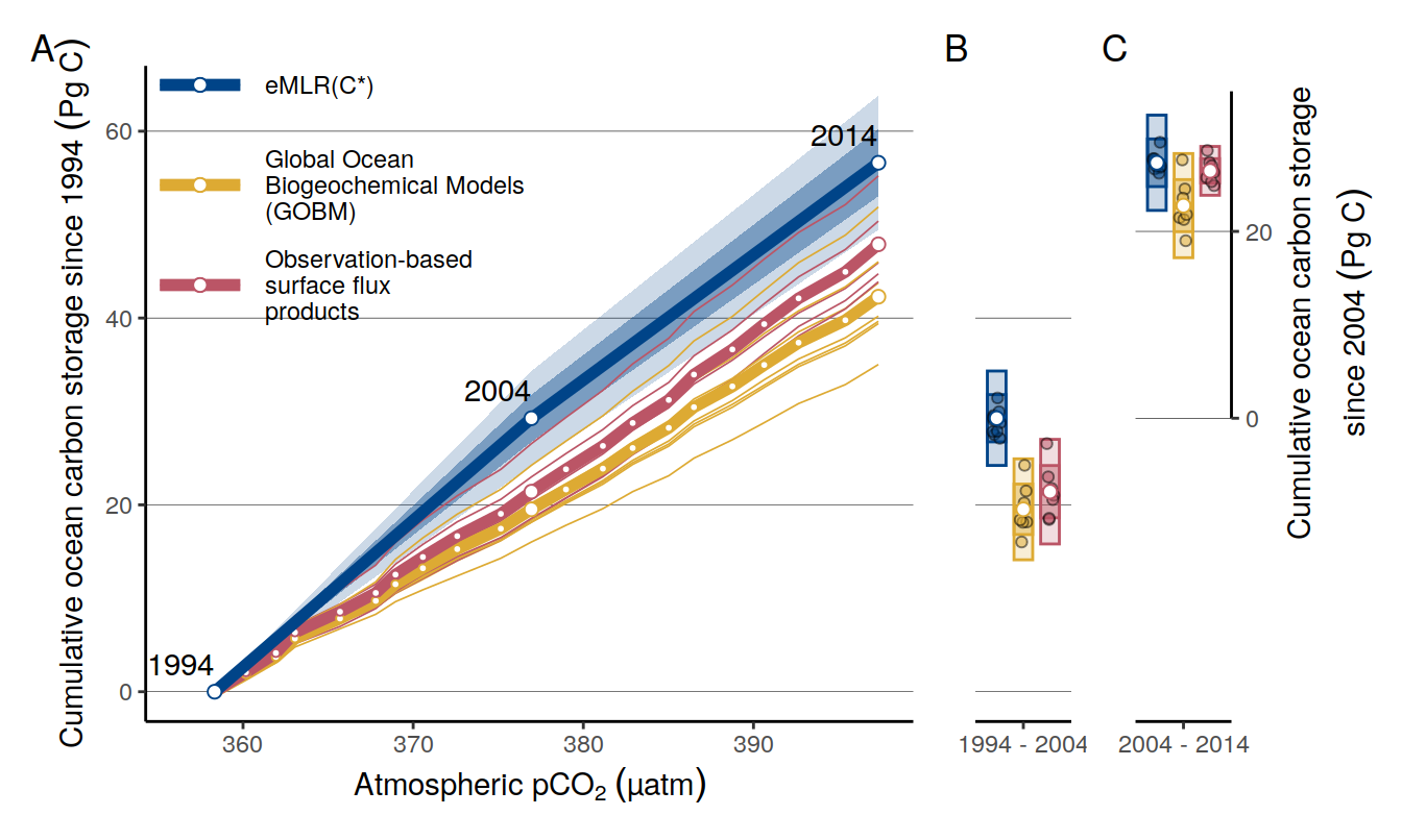
| Version | Author | Date |
|---|---|---|
| 2cca4eb | jens-daniel-mueller | 2023-01-10 |
| b9d5a73 | jens-daniel-mueller | 2022-12-15 |
| 0f2c9d5 | jens-daniel-mueller | 2022-12-08 |
| 322b1c1 | jens-daniel-mueller | 2022-11-25 |
| 491f8b1 | jens-daniel-mueller | 2022-11-25 |
| 4da4d66 | jens-daniel-mueller | 2022-11-25 |
| 534ee74 | jens-daniel-mueller | 2022-11-25 |
| e924c80 | jens-daniel-mueller | 2022-11-17 |
| 8e1702d | jens-daniel-mueller | 2022-11-16 |
| ea34027 | jens-daniel-mueller | 2022-11-15 |
| 8ac0da0 | jens-daniel-mueller | 2022-11-15 |
| 1dad51a | jens-daniel-mueller | 2022-11-15 |
| 375300e | jens-daniel-mueller | 2022-11-14 |
| ebc85e2 | jens-daniel-mueller | 2022-11-14 |
| 6edad9b | jens-daniel-mueller | 2022-11-11 |
| 16beb51 | jens-daniel-mueller | 2022-11-08 |
| b92657d | jens-daniel-mueller | 2022-11-08 |
| 7275091 | jens-daniel-mueller | 2022-11-05 |
| 99610ed | jens-daniel-mueller | 2022-11-01 |
| 7060801 | jens-daniel-mueller | 2022-10-31 |
| ecb84c1 | jens-daniel-mueller | 2022-10-30 |
| 2345935 | jens-daniel-mueller | 2022-10-29 |
| 0b40366 | jens-daniel-mueller | 2022-10-26 |
| 91052ae | jens-daniel-mueller | 2022-10-20 |
# p_tcant_ts_zoom + p_tcant_box_10 +
# plot_layout(ncol = 2, widths = c(6,1.8)) +
# plot_annotation(tag_levels = 'A')
ggsave(path = here::here("output/publication"),
filename = "Fig_dcant_inventory_global_vs_GCB_ocean_sink.png",
height = 6,
width = 8,
dpi = 600)17 Revelle changes
delta_revelle <- co2_atm %>%
mutate(revelle = seacarb::buffer(24,
pCO2,
2300 * 1e-6)$BetaD,
DIC = seacarb::carb(24,
pCO2,
2300 * 1e-6)$DIC,
delta_DIC = (1/pCO2) * DIC * (1/revelle) *1e6,
delta_DIC_rel = delta_DIC / mean(delta_DIC),
delta_DIC_rel_cum = delta_DIC_rel - first(delta_DIC_rel),
delta_year = year - first(year))
delta_revelle %>%
ggplot(aes(delta_year, pCO2)) +
geom_path() +
geom_point()
delta_revelle %>%
ggplot(aes(delta_year,1/revelle)) +
geom_smooth(method = "lm", aes(col="lm"), se = FALSE) +
geom_path() +
geom_point()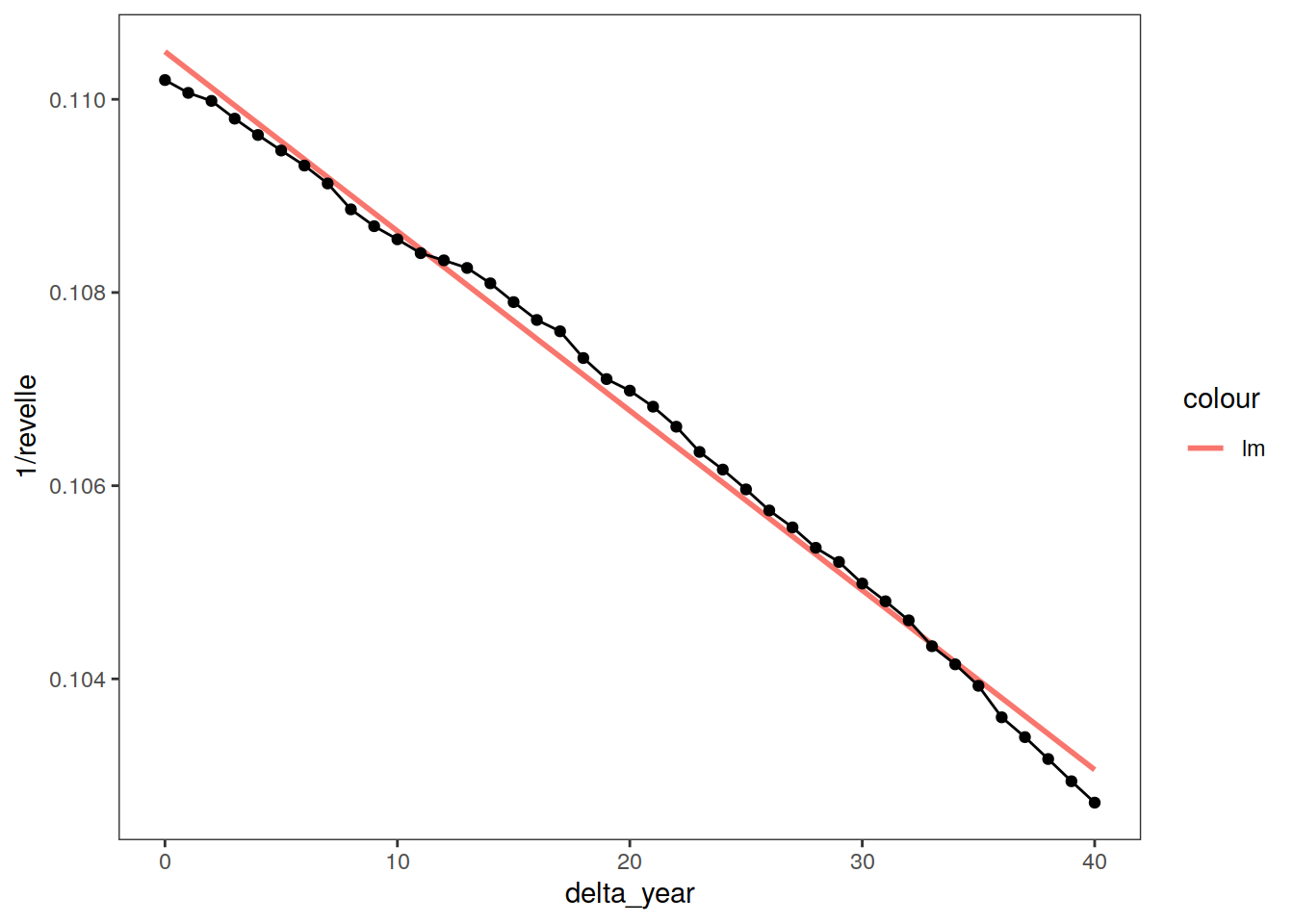
delta_revelle %>%
ggplot(aes(delta_year,delta_DIC_rel)) +
geom_smooth(method = "lm", aes(col="lm"), se = FALSE) +
geom_path() +
geom_point()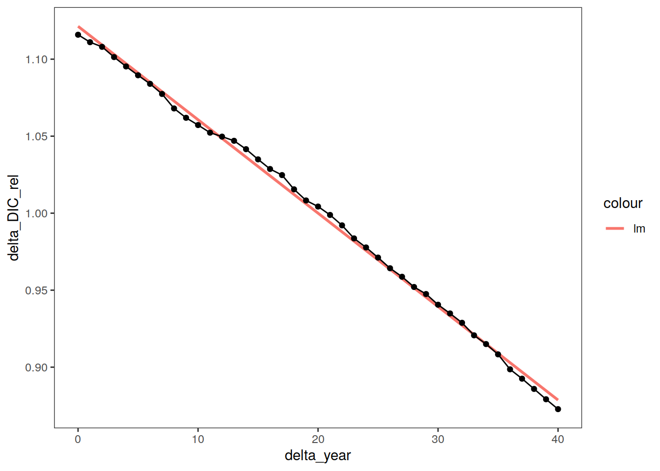
delta_revelle %>%
ggplot(aes(delta_year,delta_DIC_rel_cum)) +
geom_smooth(method = "lm", aes(col="lm"), se = FALSE) +
geom_path() +
geom_point()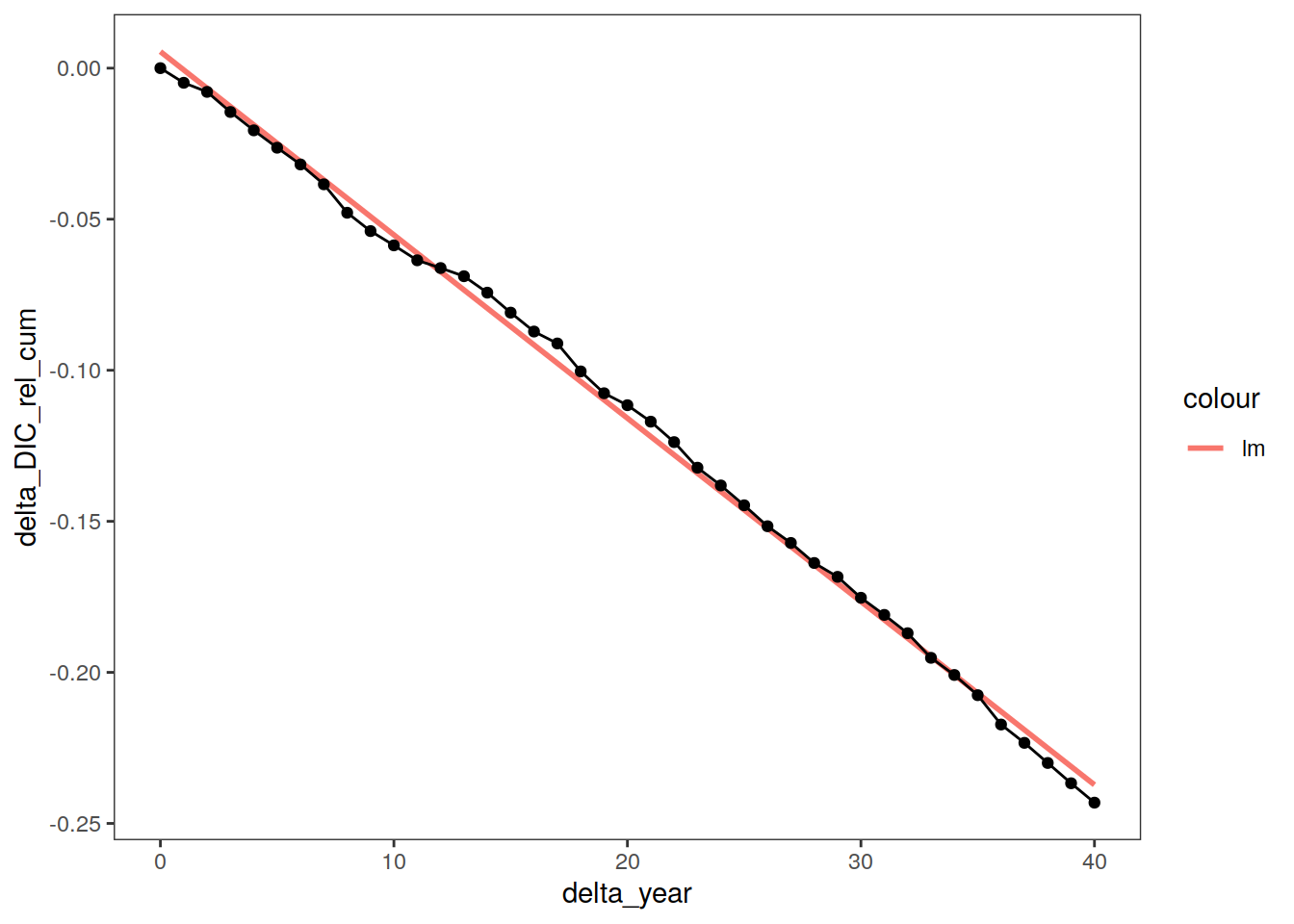
min(delta_revelle$delta_DIC_rel_cum / max(delta_revelle$delta_year))[1] -0.00607817618 GCB implications
18.1 Land sink
flux_label <- expression(CO[2]~flux~(Pg~C~yr^{-1}))
flux_components <- Global_Carbon_Budget %>%
distinct(estimate) %>%
pull()
emission_components <- flux_components[c(1,2,6)]
sink_components <- flux_components[3:5]
estimates <- Global_Carbon_Budget %>%
select(-GtC) %>%
filter(year >= 1990) %>%
pivot_wider(names_from = estimate,
values_from = GtC_yr) %>%
mutate(`fossil emissions` =
`fossil emissions excluding carbonation` - `cement carbonation sink`) %>%
select(-c(`fossil emissions excluding carbonation`, `cement carbonation sink`)) %>%
pivot_longer(-year,
names_to = "estimate",
values_to = "GtC_yr")
estimates <- estimates %>%
filter(!(estimate %in% c("budget imbalance"))) %>%
mutate(
sign = if_else(estimate %in% sink_components,
"sinks",
"emissions"),
GtC_yr = if_else(sign == "sinks",
-GtC_yr,
GtC_yr)
# GtC_yr = if_else(estimate == "cement carbonation sink",
# -GtC_yr,
# GtC_yr)
)
emissions_sinks <- estimates %>%
group_by(year, sign) %>%
summarise(GtC_yr = sum(GtC_yr)) %>%
ungroup()
estimates %>% distinct(estimate) %>% pull()[1] "land-use change emissions" "atmospheric growth"
[3] "ocean sink" "land sink"
[5] "fossil emissions" p_stacked_fluxes <- estimates %>%
mutate(
estimate = fct_relevel(
estimate,
"fossil emissions",
"land-use change emissions",
"atmospheric growth",
"land sink",
"ocean sink"
)
) %>%
ggplot() +
geom_area(aes(year, GtC_yr, fill = estimate),
col = "black",
alpha = 0.7,
size = 0.5) +
# geom_line(data = emissions_sinks %>% mutate(GtC_yr = if_else(sign == "emissions",
# -GtC_yr,
# GtC_yr)),
# aes(year, GtC_yr, linetype = sign)) +
scale_fill_manual(values = c("#BBBBBB", "#CCBB44", "#66CCEE", "#228833", "#4477AA"),
name = "flux component") +
geom_hline(yintercept = 0) +
scale_x_continuous(expand = c(0,0)) +
labs(y = flux_label,
title = "Carbon emissions and sinks",
subtitle = "Global Carbon Budget | Friedlingstein et al. (2021)") +
theme(axis.title.x = element_blank())
p_stacked_fluxes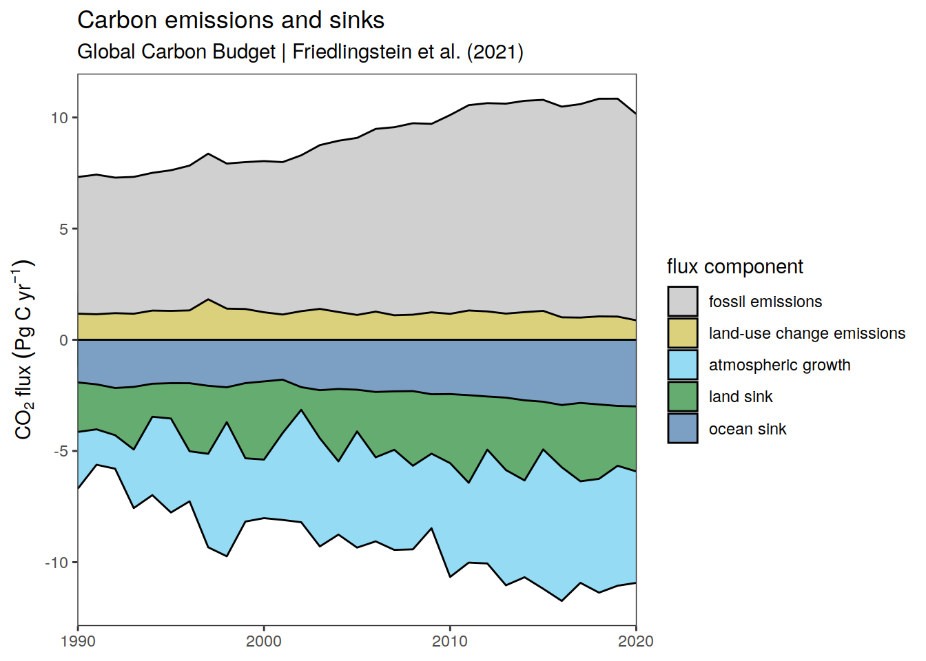
ggsave(path = here::here("output/presentation"),
filename = "Fig_GCB_emissions_sinks.png",
height = 4,
width = 7)
p_individual_fluxes <- estimates %>%
ggplot(aes(year, GtC_yr, col = estimate)) +
geom_hline(yintercept = 0) +
geom_path() +
geom_point(size = 0.5) +
scale_x_continuous(expand = c(0, 0)) +
scale_color_bright(name = "flux component") +
labs(y = flux_label,
title = "Individual flux components from GCB") +
theme(axis.title.x = element_blank())
p_individual_fluxes
BIM <- emissions_sinks %>%
pivot_wider(names_from = sign,
values_from = GtC_yr) %>%
mutate(BIM = emissions + sinks)
p_BIM <- ggplot() +
geom_line(data = Global_Carbon_Budget %>%
filter(estimate == "budget imbalance",
year >= 1994,
year < 2014),
aes(year, GtC_yr, col = "reported")) +
geom_line(data = BIM, aes(year, BIM, col = "recalculated")) +
geom_hline(yintercept = 0) +
scale_color_brewer(palette = "Set1") +
scale_x_continuous(expand = c(0, 0)) +
labs(y = flux_label,
title = "BIM from GCB") +
theme(axis.title.x = element_blank(),
legend.title = element_blank())
p_BIM
p_land_sink_gcb <- estimates %>%
select(year, estimate, GtC_yr) %>%
pivot_wider(names_from = estimate,
values_from = GtC_yr) %>%
mutate(`land sink residual` =
`fossil emissions` +
`land-use change emissions` +
`atmospheric growth` +
`ocean sink`) %>%
ggplot() +
geom_line(aes(year, -`land sink residual`, col = "residual")) +
geom_line(aes(year, `land sink`, col = "reported")) +
scale_x_continuous(expand = c(0, 0)) +
scale_color_brewer(palette = "Set1", name = "land sink\nestimate") +
labs(y = flux_label,
title = "Land sink estimates from GCB",
subtitle = "Note: The offset between reported and residual estimate equals BIM") +
theme(axis.title.x = element_blank(),
legend.title = element_blank())
p_land_sink_gcb
# Ocean_Sink %>% distinct(product)
Ocean_Sink_annual_mean <- Ocean_Sink %>%
filter(year >= 1990) %>%
group_by(year, type) %>%
summarise(GtC_yr = -mean(GtC_yr)) %>%
ungroup()
Ocean_Sink_annual_mean <- Ocean_Sink_annual_mean %>%
pivot_wider(names_from = type,
values_from = GtC_yr,
names_prefix = "ocean_sink_")
estimates_wide <- estimates %>%
select(year, estimate, GtC_yr) %>%
pivot_wider(names_from = estimate,
values_from = GtC_yr)
estimates_wide <-
full_join(estimates_wide, Ocean_Sink_annual_mean)
dcant_interior <- tcant_ts_zoom %>%
filter(year > 2000) %>%
mutate(dcant_mean = dcant_mean/10) %>%
pull(dcant_mean)
cnat <-
dcant_type_significance %>%
filter(type == "Observation-based\nsurface flux\nproducts" ,
period %in% two_decades) %>%
mutate(dcant_diff = dcant_diff/10) %>%
pull(dcant_diff)
estimates_wide <- estimates_wide %>%
mutate(ocean_sink_interior_Cant = case_when(
between(year, 1995, 2004) ~ -dcant_interior[1],
between(year, 2005, 2014) ~ -dcant_interior[2],
TRUE ~ NaN
)) %>%
mutate(ocean_sink_interior_Cnet = case_when(
between(year, 1995, 2004) ~ -dcant_interior[1]-cnat[1],
between(year, 2005, 2014) ~ -dcant_interior[2]-cnat[2],
TRUE ~ NaN
)) %>%
mutate(ocean_sink_interior_Cnat = case_when(
between(year, 1995, 2004) ~ -cnat[1],
between(year, 2005, 2014) ~ -cnat[2],
TRUE ~ NaN
))
p_ocean_sinks <- estimates_wide %>%
select(year, starts_with("ocean")) %>%
rename(GCB_mean = `ocean sink`) %>%
pivot_longer(-year,
names_to = "estimate",
names_prefix = "ocean_sink_",
values_to = "GtC_yr") %>%
mutate(estimate = str_replace(estimate, "_", " ")) %>%
ggplot(aes(year, GtC_yr, col = estimate)) +
geom_path() +
geom_point(size = 0.5) +
scale_x_continuous(expand = c(0, 0)) +
scale_color_brewer(palette = "Dark2", name = "ocean sink\nestimate") +
labs(y = flux_label,
title = "Ocean sink estimates",
subtitle = "Note: Watson et al. (2020) is excluded in data products and GCB mean") +
theme(axis.title.x = element_blank(),
legend.title = element_blank())
p_ocean_sinks
| Version | Author | Date |
|---|---|---|
| 445761e | jens-daniel-mueller | 2022-12-02 |
| 439cb85 | jens-daniel-mueller | 2022-11-29 |
| 9048dc4 | jens-daniel-mueller | 2022-11-29 |
| 3a7bab0 | jens-daniel-mueller | 2022-11-28 |
| ea34027 | jens-daniel-mueller | 2022-11-15 |
| 1dad51a | jens-daniel-mueller | 2022-11-15 |
| 6edad9b | jens-daniel-mueller | 2022-11-11 |
| 7275091 | jens-daniel-mueller | 2022-11-05 |
| 2345935 | jens-daniel-mueller | 2022-10-29 |
| 91052ae | jens-daniel-mueller | 2022-10-20 |
estimates_long <- estimates_wide %>%
select(year, starts_with("ocean")) %>%
rename(GCB_mean = `ocean sink`) %>%
pivot_longer(-year,
names_to = "estimate",
names_prefix = "ocean_sink_",
values_to = "GtC_yr") %>%
filter(estimate %in% c("data_products", "models"),
year >= 1990)
p_ocean_sinks_presentation <- estimates_long %>%
# mutate(estimate = str_replace(estimate, "_", " ")) %>%
ggplot() +
geom_path(data = Ocean_Sink %>% filter(year >= 1990),
aes(year, GtC_yr, group = product, col = type), size = 0.3) +
geom_path(aes(year, -GtC_yr, col = estimate), size = 2) +
geom_point(aes(year, -GtC_yr, col = estimate), size = 2, fill = "white", shape = 21) +
scale_x_continuous(expand = c(0, 0)) +
scale_color_manual(values = c("#BB5566", "#DDAA33"),
name = "ocean sink\nestimate") +
labs(y = flux_label,
title = "Ocean Carbon sink",
subtitle = "Global Carbon Budget | Friedlingstein et al. (2021)") +
theme(axis.title.x = element_blank(),
legend.title = element_blank())
p_ocean_sinks_presentation
ggsave(path = here::here("output/presentation"),
filename = "Fig_GCB_ocean_sinks.png",
height = 4,
width = 6)
p_ocean_sinks_presentation <-
estimates_long %>%
# mutate(estimate = str_replace(estimate, "_", " ")) %>%
ggplot() +
geom_path(
data = Ocean_Sink %>% filter(year >= 1990),
aes(year, GtC_yr, group = product, col = type),
size = 0.3
) +
geom_path(aes(year, -GtC_yr, col = estimate), size = 2) +
geom_point(
aes(year, -GtC_yr, col = estimate),
size = 2,
fill = "white",
shape = 21
) +
geom_path(
data = tibble(
year = c(1994, 2007),
estimate = "ocean_interior",
GtC_yr = -2.6
),
aes(year, -GtC_yr, col = estimate),
size = 2
)+
geom_rect(
data = tibble(
year_min = 1994,
year_max = 2007,
estimate = "ocean_interior",
GtC_yr_min = -2.6 - 0.3,
GtC_yr_max = -2.6 + 0.3,
),
aes(xmax = year_max, xmin = year_min, ymin = -GtC_yr_min, ymax = -GtC_yr_max, col = estimate),
fill = "transparent"
)+
scale_x_continuous(expand = c(0, 0)) +
scale_color_manual(values = c("#BB5566", "#DDAA33","#004488"),
name = "ocean sink\nestimate") +
labs(y = flux_label,
title = "Ocean Carbon sink",
subtitle = "Global Carbon Budget | Friedlingstein et al. (2021)") +
theme(axis.title.x = element_blank(),
legend.title = element_blank())
p_ocean_sinks_presentation
ggsave(path = here::here("output/presentation"),
filename = "Fig_GCB_ocean_sinks_eMLR.png",
height = 4,
width = 6)
land_sink <-
estimates_wide %>%
mutate(emissions_atmosphere = `fossil emissions` +
`land-use change emissions` +
`atmospheric growth`) %>%
rename(ocean_sink_gcb_mean = `ocean sink`) %>%
select(year, emissions_atmosphere, starts_with("ocean")) %>%
pivot_longer(
starts_with("ocean_sink"),
names_to = "ocean_sink_estimate",
values_to = "ocean_sink",
names_prefix = "ocean_sink_"
) %>%
mutate(land_sink = -emissions_atmosphere - ocean_sink)
p_land_sink <- land_sink %>%
mutate(ocean_sink_estimate =
str_replace(ocean_sink_estimate, "_", " ")) %>%
ggplot() +
geom_hline(yintercept = 0) +
geom_line(aes(year, land_sink, col = ocean_sink_estimate, linetype = "residual\nestimate")) +
geom_line(data = estimates_wide,
aes(year, `land sink`, linetype = "direct\nestimate", col = "reported land sink")) +
scale_x_continuous(expand = c(0, 0)) +
scale_linetype_manual(values = c(2, 1), name = "land sink\nestimate") +
scale_color_brewer(palette = "Dark2",
name = "ocean sink\nestimate\nunderlying\nresidual\nestimate") +
guides(linetype = guide_legend(order = 1),
color = guide_legend(order = 2)) +
labs(y = flux_label,
title = "Land sink estimates",
subtitle = "Residuals estimates are determined for a range of ocean sink estimates") +
theme(axis.title.x = element_blank())
p_land_sink
| Version | Author | Date |
|---|---|---|
| 445761e | jens-daniel-mueller | 2022-12-02 |
| 439cb85 | jens-daniel-mueller | 2022-11-29 |
| 9048dc4 | jens-daniel-mueller | 2022-11-29 |
| 3a7bab0 | jens-daniel-mueller | 2022-11-28 |
| ea34027 | jens-daniel-mueller | 2022-11-15 |
| 1dad51a | jens-daniel-mueller | 2022-11-15 |
| 6edad9b | jens-daniel-mueller | 2022-11-11 |
| 7275091 | jens-daniel-mueller | 2022-11-05 |
| 2345935 | jens-daniel-mueller | 2022-10-29 |
| 91052ae | jens-daniel-mueller | 2022-10-20 |
land_sink_long <-
full_join(
land_sink %>%
select(year, ocean_sink_estimate, land_sink),
estimates_wide %>%
select(year, land_sink = `land sink`) %>%
mutate(ocean_sink_estimate = "reported_land_sink")
)
land_sink_long_decade <- land_sink_long %>%
mutate(period = cut(year, c(1993, 2003, 2013),
c("1994 - 2004", "2004 - 2014"))) %>%
filter(!is.na(period)) %>%
group_by(ocean_sink_estimate, period) %>%
summarise(across(starts_with("land_sink"), list(mean = mean, sd = sd))) %>%
ungroup() %>%
mutate(ocean_sink_estimate =
str_replace_all(ocean_sink_estimate, "_", " "))
land_sink_long_decade# A tibble: 14 × 4
ocean_sink_estimate period land_sink_mean land_sink_sd
<chr> <fct> <dbl> <dbl>
1 data products 1994 - 2004 -1.96 1.19
2 data products 2004 - 2014 -2.96 0.789
3 gcb mean 1994 - 2004 -2.07 1.19
4 gcb mean 2004 - 2014 -3.16 0.800
5 interior Cant 1994 - 2004 NaN NA
6 interior Cant 2004 - 2014 -2.80 0.837
7 interior Cnat 1994 - 2004 NaN NA
8 interior Cnat 2004 - 2014 -5.71 0.876
9 interior Cnet 1994 - 2004 NaN NA
10 interior Cnet 2004 - 2014 -2.96 0.860
11 models 1994 - 2004 -2.15 1.21
12 models 2004 - 2014 -3.32 0.818
13 reported land sink 1994 - 2004 -2.33 0.892
14 reported land sink 2004 - 2014 -2.94 0.578p_land_sink_decade <-
land_sink_long_decade %>%
ggplot() +
geom_hline(yintercept = 0) +
geom_pointrange(
aes(
period,
land_sink_mean,
ymin = land_sink_mean - land_sink_sd,
ymax = land_sink_mean + land_sink_sd,
col = ocean_sink_estimate
),
position = position_dodge2(width = 0.5)
) +
scale_color_brewer(palette = "Dark2",
name = "ocean sink\nestimate\nunderlying\nresidual\nestimate") +
guides(shape = guide_legend(order = 1),
color = guide_legend(order = 2)) +
theme(axis.title.x = element_blank()) +
labs(y = flux_label,
title = "Decadal mean land sink estimates",
subtitle = "Errorbars indicate the StDev of the interannual variability") +
theme(axis.title.x = element_blank())
p_land_sink_decade
| Version | Author | Date |
|---|---|---|
| 445761e | jens-daniel-mueller | 2022-12-02 |
| 9048dc4 | jens-daniel-mueller | 2022-11-29 |
| 3a7bab0 | jens-daniel-mueller | 2022-11-28 |
| ea34027 | jens-daniel-mueller | 2022-11-15 |
| 1dad51a | jens-daniel-mueller | 2022-11-15 |
| 6edad9b | jens-daniel-mueller | 2022-11-11 |
| 7275091 | jens-daniel-mueller | 2022-11-05 |
| 2345935 | jens-daniel-mueller | 2022-10-29 |
| 91052ae | jens-daniel-mueller | 2022-10-20 |
land_sink <-
full_join(
land_sink,
estimates_wide %>%
select(year, land_sink_reported = `land sink`)
)
p_land_sink_residual <- land_sink %>%
mutate(ocean_sink_estimate =
str_replace(ocean_sink_estimate, "_", " ")) %>%
ggplot() +
geom_hline(yintercept = 0) +
geom_line(aes(year, land_sink - land_sink_reported, col = ocean_sink_estimate)) +
scale_x_continuous(expand = c(0, 0)) +
scale_color_brewer(palette = "Dark2",
name = "ocean sink\nestimate\nunderlying\nresidual") +
labs(y = flux_label,
title = "Land sink estimates (reported - residual)",
subtitle = "Residuals are determined for a range of ocean sink estimates") +
theme(axis.title.x = element_blank())
p_land_sink_residual
| Version | Author | Date |
|---|---|---|
| 445761e | jens-daniel-mueller | 2022-12-02 |
| 439cb85 | jens-daniel-mueller | 2022-11-29 |
| 9048dc4 | jens-daniel-mueller | 2022-11-29 |
| 3a7bab0 | jens-daniel-mueller | 2022-11-28 |
| ea34027 | jens-daniel-mueller | 2022-11-15 |
| 1dad51a | jens-daniel-mueller | 2022-11-15 |
| 6edad9b | jens-daniel-mueller | 2022-11-11 |
| 7275091 | jens-daniel-mueller | 2022-11-05 |
| 2345935 | jens-daniel-mueller | 2022-10-29 |
| 91052ae | jens-daniel-mueller | 2022-10-20 |
p_land_sink_residual_decade <- land_sink %>%
mutate(period = cut(year, c(1993, 2003, 2013),
c("1994 - 2004", "2004 - 2014"))) %>%
filter(!is.na(period)) %>%
mutate(land_sink_residual = land_sink - land_sink_reported) %>%
select(period, ocean_sink_estimate, land_sink_residual) %>%
group_by(ocean_sink_estimate, period) %>%
summarise(across(starts_with("land_sink"), list(mean = mean, sd = sd))) %>%
ungroup() %>%
mutate(ocean_sink_estimate =
str_replace(ocean_sink_estimate, "_", " ")) %>%
ggplot() +
geom_hline(yintercept = 0) +
geom_pointrange(
aes(
period,
land_sink_residual_mean,
ymin = land_sink_residual_mean - land_sink_residual_sd,
ymax = land_sink_residual_mean + land_sink_residual_sd,
col = ocean_sink_estimate
),
position = position_dodge2(width = 0.5)
) +
scale_color_brewer(palette = "Dark2",
name = "ocean sink\nestimate\nunderlying\nresidual") +
theme(axis.title.x = element_blank()) +
labs(y = flux_label,
title = "Decadal mean land sink estimates",
subtitle = "Errorbars indicate the StDev of the interannual variability") +
theme(axis.title.x = element_blank())
p_land_sink_residual_decade
BIM_ocean <- land_sink %>%
mutate(BIM = emissions_atmosphere + ocean_sink + land_sink_reported)
p_BIM_ocean <- BIM_ocean %>%
mutate(ocean_sink_estimate =
str_replace(ocean_sink_estimate, "_", " ")) %>%
ggplot() +
geom_hline(yintercept = 0) +
geom_line(aes(year, BIM, col = ocean_sink_estimate)) +
scale_x_continuous(expand = c(0, 0)) +
scale_color_brewer(palette = "Dark2",
name = "ocean sink\nestimate\nunderlying\nBIM") +
labs(y = flux_label,
title = "BIM estimates",
subtitle = "BIM estimates are determined for a range of ocean sink estimates") +
theme(axis.title.x = element_blank())
p_BIM_ocean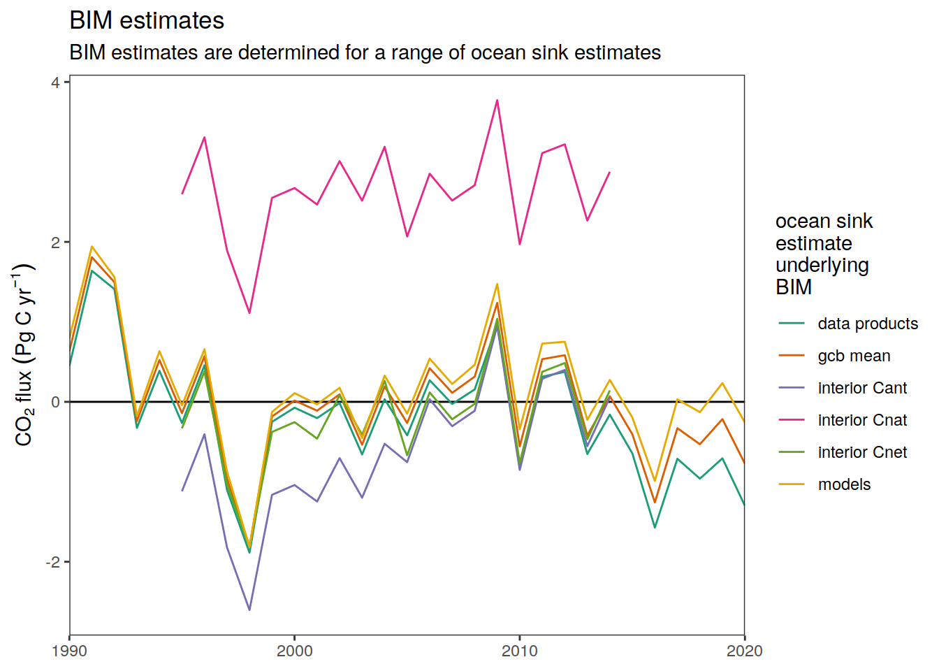
BIM_ocean_decade <- BIM_ocean %>%
mutate(period = cut(year, c(1993, 2003, 2013),
c("1994 - 2004", "2004 - 2014"))) %>%
filter(!is.na(period)) %>%
group_by(ocean_sink_estimate, period) %>%
summarise(across(starts_with("BIM"), list(mean = mean, sd = sd))) %>%
ungroup() %>%
mutate(ocean_sink_estimate =
str_replace_all(ocean_sink_estimate, "_", " "))
BIM_ocean_decade# A tibble: 12 × 4
ocean_sink_estimate period BIM_mean BIM_sd
<chr> <fct> <dbl> <dbl>
1 data products 1994 - 2004 -0.361 0.703
2 data products 2004 - 2014 0.0208 0.530
3 gcb mean 1994 - 2004 -0.254 0.709
4 gcb mean 2004 - 2014 0.215 0.535
5 interior Cant 1994 - 2004 NaN NA
6 interior Cant 2004 - 2014 -0.143 0.570
7 interior Cnat 1994 - 2004 NaN NA
8 interior Cnat 2004 - 2014 2.77 0.573
9 interior Cnet 1994 - 2004 NaN NA
10 interior Cnet 2004 - 2014 0.0134 0.561
11 models 1994 - 2004 -0.177 0.734
12 models 2004 - 2014 0.379 0.546p_BIM_ocean_decade <-
BIM_ocean_decade %>%
ggplot() +
geom_hline(yintercept = 0) +
geom_pointrange(
aes(
period,
BIM_mean,
ymin = BIM_mean - BIM_sd,
ymax = BIM_mean + BIM_sd,
col = ocean_sink_estimate
),
position = position_dodge2(width = 0.5)
) +
scale_color_brewer(palette = "Dark2",
name = "ocean sink\nestimate\nunderlying\nBIM") +
guides(shape = guide_legend(order = 1),
color = guide_legend(order = 2)) +
theme(axis.title.x = element_blank()) +
labs(y = flux_label,
title = "Decadal mean BIM estimates",
subtitle = "Errorbars indicate the StDev of the interannual variability") +
theme(axis.title.x = element_blank())
p_BIM_ocean_decade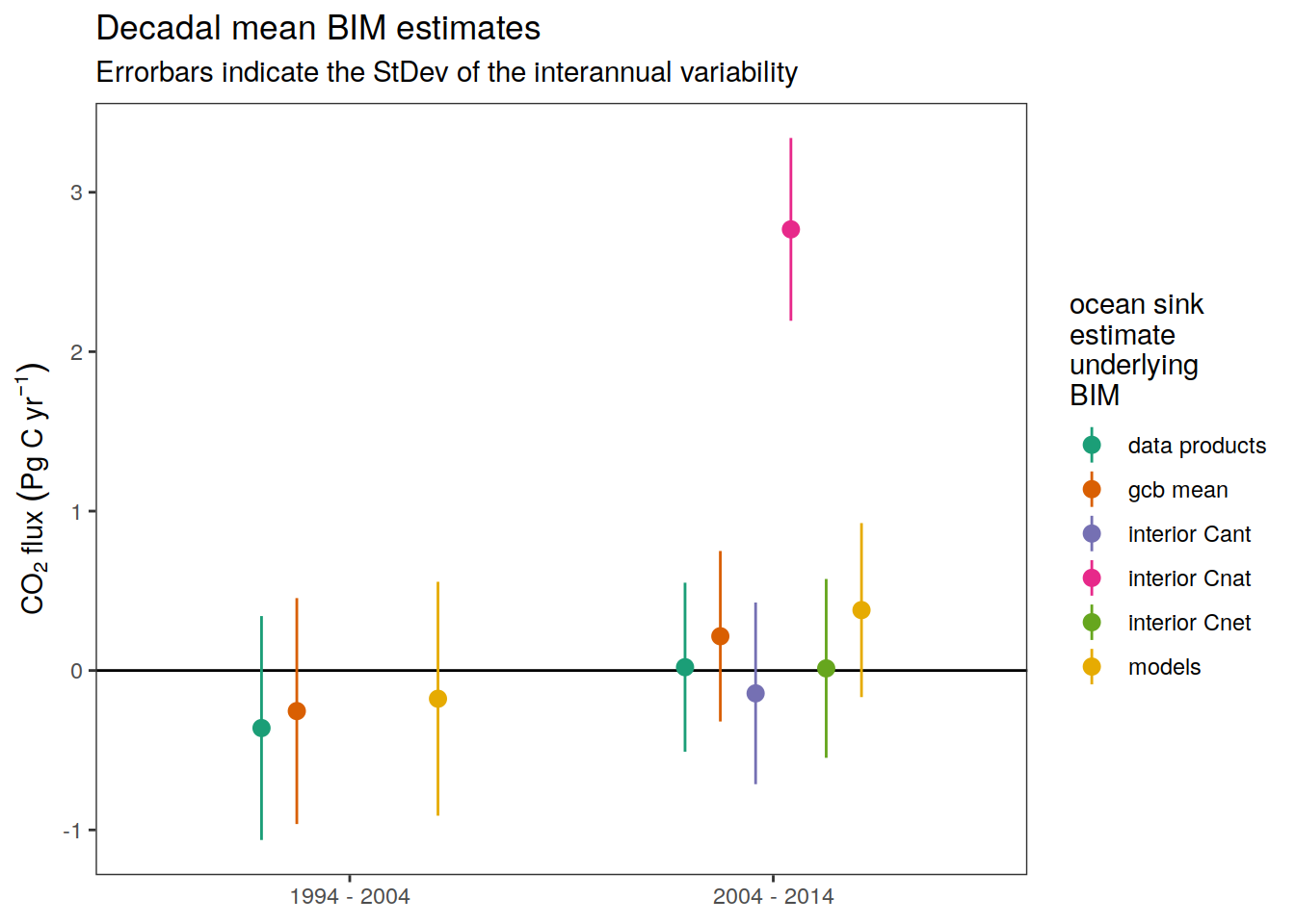
pdf(
file = here::here("output/publication/GCB_land_sink_and_BIM.pdf"),
height = 4,
width = 8
)
# p_stacked_fluxes
p_individual_fluxes
# p_BIM
# p_land_sink_gcb
p_ocean_sinks
p_land_sink
p_land_sink_decade
# p_land_sink_residual
# p_land_sink_residual_decade
p_BIM_ocean
p_BIM_ocean_decade
dev.off()png
2 rm(
p_stacked_fluxes,
p_individual_fluxes,
p_BIM,
p_land_sink_gcb,
p_ocean_sinks,
p_land_sink,
p_land_sink_decade,
p_land_sink_residual,
p_land_sink_residual_decade,
p_BIM_ocean,
p_BIM_ocean_decade,
estimates,
# estimates_wide,
land_sink,
land_sink_long,
land_sink_long_decade,
Ocean_Sink_annual_mean,
flux_components,
flux_label,
emission_components,
sink_components
)18.1.1 Decadal Budgets
Decadal_GCB_budgets <- estimates_wide %>%
pivot_longer(-year,
names_to = "CO2_sources_sinks",
values_to = "GtC_yr") %>%
mutate(period = cut(year, c(1994, 2004, 2014), c("1994 - 2004", "2004 - 2014"))) %>%
drop_na() %>%
group_by(period, CO2_sources_sinks) %>%
summarise(GtC = sum(GtC_yr)) %>%
ungroup()
Decadal_GCB_budgets <- Decadal_GCB_budgets %>%
filter(
!(CO2_sources_sinks %in% c("ocean_sink_data_products", "ocean sink", "ocean_sink_models"))
) %>%
mutate(CO2_sources_sinks = str_remove(CO2_sources_sinks, "_interior"))
total_emissions <- Decadal_GCB_budgets %>%
filter(
CO2_sources_sinks %in% c("fossil emissions", "land-use change emissions")
) %>%
group_by(period) %>%
summarise(GtC = sum(GtC)) %>%
ungroup() %>%
mutate(CO2_sources_sinks = "total emissions")
Decadal_GCB_budgets <- full_join(Decadal_GCB_budgets, total_emissions)
ocean_stats <- dcant_type_box_stat %>%
filter(period %in% two_decades) %>%
mutate(type = case_when(
type == "eMLR(C*)" ~ "ocean_sink_Cant",
type == "Observation-based\nsurface flux\nproducts" ~ "ocean_sink_Cnet",
TRUE ~ "x"
)) %>%
filter(type != "x") %>%
select(period, CO2_sources_sinks = type, GtC_sigma = dcant_sd)
Decadal_GCB_budgets <-
full_join(Decadal_GCB_budgets,
ocean_stats)
rm(ocean_stats)
ocean_stats <- dcant_type_significance %>%
filter(period %in% two_decades) %>%
mutate(type = case_when(
type == "Observation-based\nsurface flux\nproducts" ~ "ocean_sink_Cnat",
TRUE ~ "x"
)) %>%
filter(type != "x") %>%
select(period, CO2_sources_sinks = type, GtC_sigma = dcant_diff_sd)
library(rqdatatable)
Decadal_GCB_budgets <-
natural_join(
Decadal_GCB_budgets,
ocean_stats,
by = c("period", "CO2_sources_sinks"),
jointype = "FULL"
)
rm(ocean_stats)
Decadal_GCB_budgets <- Decadal_GCB_budgets %>%
mutate(GtC_sigma = case_when(
CO2_sources_sinks == "fossil emissions" ~ GtC * 0.4 / 7.7,
CO2_sources_sinks == "land-use change emissions" ~ GtC * 0.7 / 1.2,
CO2_sources_sinks == "total emissions" ~ GtC * 0.8 / 9.0,
CO2_sources_sinks == "atmospheric growth" ~ GtC * 0.02 / 4.0,
CO2_sources_sinks == "land sink" ~ GtC * 0.5 / 2.6,
TRUE ~ GtC_sigma
)) %>%
mutate(GtC_sigma = abs(GtC_sigma))
Decadal_GCB_budgets %>%
ggplot(aes(period, GtC,
ymin = GtC - GtC_sigma,
ymax = GtC + GtC_sigma,
col = CO2_sources_sinks)) +
geom_hline(yintercept = 0) +
scale_color_muted() +
geom_pointrange(position = position_dodge2(width = 0.5),
shape = 1)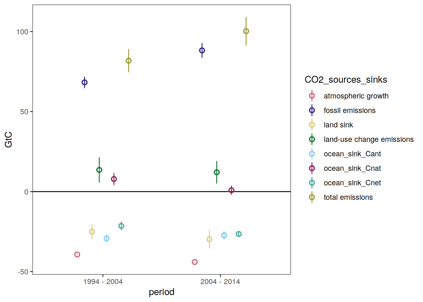
| Version | Author | Date |
|---|---|---|
| 445761e | jens-daniel-mueller | 2022-12-02 |
Decadal_GCB_fractions <- Decadal_GCB_budgets
Decadal_GCB_budgets <- Decadal_GCB_budgets %>%
mutate(across(where(is.numeric), round, 1)) %>%
mutate(GtC = paste(GtC, GtC_sigma, sep = " ± ")) %>%
select(-GtC_sigma) %>%
pivot_wider(names_from = period,
values_from = GtC) %>%
mutate(CO2_sources_sinks = str_replace_all(CO2_sources_sinks, "_", " "))
Decadal_GCB_budgets %>%
write_csv(here::here("output/publication/Table_GCB.csv"))
Decadal_GCB_fractions <- Decadal_GCB_fractions %>%
filter(CO2_sources_sinks %in% c("atmospheric growth", "land sink",
"ocean_sink_Cnet", "ocean_sink_Cant",
"total emissions")) %>%
group_by(period) %>%
mutate(fraction = abs(GtC / last(GtC))*100,
GtC_rel = abs(GtC_sigma / GtC),
fraction_rel = sqrt(GtC_rel^2 + last(GtC_rel)^2),
fraction_sigma = fraction_rel * fraction) %>%
ungroup() %>%
select(period, CO2_sources_sinks, fraction, fraction_sigma) %>%
mutate(across(where(is.numeric), round, 0)) %>%
mutate(fraction = paste0(fraction, " ± ", fraction_sigma)) %>%
select(-fraction_sigma) %>%
filter(CO2_sources_sinks != "total emissions") %>%
pivot_wider(names_from = period,
values_from = fraction) %>%
mutate(CO2_sources_sinks = str_replace_all(CO2_sources_sinks, "_", " "))
Decadal_GCB_fractions# A tibble: 4 × 3
CO2_sources_sinks `1994 - 2004` `2004 - 2014`
<chr> <chr> <chr>
1 atmospheric growth 48 ± 4 44 ± 4
2 land sink 31 ± 6 30 ± 6
3 ocean sink Cant 36 ± 4 27 ± 4
4 ocean sink Cnet 26 ± 4 26 ± 3 Decadal_GCB_fractions %>%
write_csv(here::here("output/publication/Table_GCB_fraction.csv"))18.2 Net land sink
flux_label <- expression(flux~(Pg~C~yr^{-1}))
Global_Carbon_Budget_net_land_sink <- Global_Carbon_Budget %>%
select(year, estimate, GtC_yr) %>%
pivot_wider(names_from = estimate,
values_from = GtC_yr) %>%
mutate(`net land sink` = `land sink` - `land-use change emissions`) %>%
select(-c(`land sink`, `land-use change emissions`)) %>%
pivot_longer(-year,
names_to = "estimate",
values_to = "GtC_yr")
flux_components <- Global_Carbon_Budget_net_land_sink %>%
distinct(estimate) %>%
pull()
emission_components <- flux_components[c(1,4)]
sink_components <- flux_components[c(2,3,6)]
estimates <- Global_Carbon_Budget_net_land_sink %>%
filter(!(estimate %in% c("budget imbalance")),
year >= 1990) %>%
mutate(
sign = if_else(estimate %in% sink_components,
"sinks",
"emissions"),
GtC_yr = if_else(sign == "sinks",
-GtC_yr,
GtC_yr),
GtC_yr = if_else(estimate == "cement carbonation sink",
-GtC_yr,
GtC_yr)
)
emissions_sinks <- estimates %>%
group_by(year, sign) %>%
summarise(GtC_yr = sum(GtC_yr)) %>%
ungroup()
p_stacked_fluxes <- estimates %>%
ggplot() +
geom_area(aes(year, GtC_yr, fill = estimate),
col = "white",
alpha = 0.7,
size = 0.5) +
geom_line(data = emissions_sinks %>% mutate(GtC_yr = if_else(sign == "emissions",
-GtC_yr,
GtC_yr)),
aes(year, GtC_yr, linetype = sign)) +
scale_fill_bright(name = "flux component") +
geom_hline(yintercept = 0) +
scale_x_continuous(expand = c(0,0)) +
labs(y = flux_label,
title = "Stacked emission and sink components from GCB",
subtitle = "Note: The cement carbonation sink is accounted for in emissions") +
theme(axis.title.x = element_blank())
p_stacked_fluxes
p_individual_fluxes <- estimates %>%
ggplot(aes(year, GtC_yr, col = estimate)) +
geom_hline(yintercept = 0) +
geom_path() +
geom_point(size = 0.5) +
scale_x_continuous(expand = c(0, 0)) +
scale_color_bright(name = "flux component") +
labs(y = flux_label,
title = "Individual flux components from GCB") +
theme(axis.title.x = element_blank())
p_individual_fluxes
BIM <- emissions_sinks %>%
pivot_wider(names_from = sign,
values_from = GtC_yr) %>%
mutate(BIM = emissions + sinks)
p_BIM <- ggplot() +
geom_line(data = Global_Carbon_Budget %>%
filter(estimate == "budget imbalance",
year >= 1990),
aes(year, GtC_yr, col = "reported")) +
geom_line(data = BIM, aes(year, BIM, col = "recalculated")) +
geom_hline(yintercept = 0) +
scale_color_brewer(palette = "Set1") +
scale_x_continuous(expand = c(0, 0)) +
labs(y = flux_label,
title = "BIM from GCB") +
theme(axis.title.x = element_blank(),
legend.title = element_blank())
p_BIM
p_land_sink_gcb <- estimates %>%
select(year, estimate, GtC_yr) %>%
pivot_wider(names_from = estimate,
values_from = GtC_yr) %>%
mutate(`net land sink residual` =
`fossil emissions excluding carbonation` +
`cement carbonation sink` +
`atmospheric growth` +
`ocean sink`) %>%
ggplot() +
geom_line(aes(year, -`net land sink residual`, col = "residual")) +
geom_line(aes(year, `net land sink`, col = "reported")) +
scale_x_continuous(expand = c(0, 0)) +
scale_color_brewer(palette = "Set1", name = "land sink\nestimate") +
labs(y = flux_label,
title = "Land sink estimates from GCB",
subtitle = "Note: The offset between reported and residual estimate equals BIM") +
theme(axis.title.x = element_blank(),
legend.title = element_blank())
p_land_sink_gcb
Ocean_Sink_annual_mean <- Ocean_Sink %>%
filter(year >= 1990) %>%
group_by(year, type) %>%
summarise(GtC_yr = -mean(GtC_yr)) %>%
ungroup()
Ocean_Sink_annual_mean <- Ocean_Sink_annual_mean %>%
pivot_wider(names_from = type,
values_from = GtC_yr,
names_prefix = "ocean_sink_")
estimates_wide <- estimates %>%
select(year, estimate, GtC_yr) %>%
pivot_wider(names_from = estimate,
values_from = GtC_yr)
estimates_wide <-
full_join(estimates_wide, Ocean_Sink_annual_mean)
dcant_interior <- tcant_ts_zoom %>%
filter(year > 2000) %>%
mutate(dcant_mean = dcant_mean/10) %>%
pull(dcant_mean)
cnat <-
dcant_type_significance %>%
filter(type == "Observation-based\nsurface flux\nproducts" ,
period %in% two_decades) %>%
mutate(dcant_diff = dcant_diff/10) %>%
pull(dcant_diff)
estimates_wide <- estimates_wide %>%
mutate(ocean_sink_interior_Cant = case_when(
between(year, 1994, 2003) ~ -dcant_interior[1],
between(year, 2004, 2013) ~ -dcant_interior[2],
TRUE ~ NaN
)) %>%
mutate(ocean_sink_interior_net = case_when(
between(year, 1994, 2003) ~ -dcant_interior[1]-cnat[1],
between(year, 2004, 2013) ~ -dcant_interior[2]-cnat[2],
TRUE ~ NaN
))
p_ocean_sinks <- estimates_wide %>%
select(year, starts_with("ocean")) %>%
rename(GCB_mean = `ocean sink`) %>%
pivot_longer(-year,
names_to = "estimate",
names_prefix = "ocean_sink_",
values_to = "GtC_yr") %>%
mutate(estimate = str_replace(estimate, "_", " ")) %>%
ggplot(aes(year, GtC_yr, col = estimate)) +
geom_path() +
geom_point(size = 0.5) +
scale_x_continuous(expand = c(0, 0)) +
scale_color_brewer(palette = "Set1", name = "ocean sink\nestimate") +
labs(y = flux_label,
title = "Ocean sink estimates",
subtitle = "Note: Watson et al. (2020) is included in data products and GCB mean") +
theme(axis.title.x = element_blank(),
legend.title = element_blank())
p_ocean_sinks
land_sink <-
estimates_wide %>%
mutate(emissions_atmosphere = `fossil emissions excluding carbonation` +
`atmospheric growth`) %>%
rename(ocean_sink_gcb_mean = `ocean sink`) %>%
select(year, emissions_atmosphere, starts_with("ocean")) %>%
pivot_longer(
starts_with("ocean_sink"),
names_to = "ocean_sink_estimate",
values_to = "ocean_sink",
names_prefix = "ocean_sink_"
) %>%
mutate(net_land_sink = -emissions_atmosphere - ocean_sink)
p_land_sink_residual <- land_sink %>%
mutate(ocean_sink_estimate =
str_replace(ocean_sink_estimate, "_", " ")) %>%
ggplot() +
geom_line(aes(year, net_land_sink, col = ocean_sink_estimate, linetype = "residual")) +
geom_line(data = estimates_wide %>%
filter(year >= 1990),
aes(year, `net land sink`, linetype = "reported")) +
scale_x_continuous(expand = c(0, 0)) +
scale_linetype_manual(values = c(2, 1), name = "net land sink\nestimate") +
scale_color_brewer(palette = "Set1",
name = "ocean sink\nestimate\nunderlying\nresidual") +
guides(linetype = guide_legend(order = 1),
color = guide_legend(order = 2)) +
labs(y = flux_label,
title = "Net land sink estimates",
subtitle = "Note: Residuals are determined for a range of ocean sink estimates") +
theme(axis.title.x = element_blank())
p_land_sink_residual
land_sink <-
full_join(
land_sink,
estimates_wide %>%
select(year, net_land_sink_reported = `net land sink`)
)
p_land_sink_residual_delta <- land_sink %>%
mutate(ocean_sink_estimate =
str_replace(ocean_sink_estimate, "_", " ")) %>%
ggplot() +
geom_hline(yintercept = 0) +
geom_line(aes(year, net_land_sink - net_land_sink_reported, col = ocean_sink_estimate)) +
scale_x_continuous(expand = c(0, 0)) +
scale_color_brewer(palette = "Set1",
name = "ocean sink\nestimate\nunderlying\nresidual") +
labs(y = flux_label,
title = "Let land sink estimates (reported - residual)",
subtitle = "Note: Residuals are determined for a range of ocean sink estimates") +
theme(axis.title.x = element_blank())
p_land_sink_residual_delta
p_land_sink_residual_decade <- land_sink %>%
mutate(period = cut(year, c(1993, 2003, 2013),
c("1994 - 2004", "2004 - 2014"))) %>%
filter(!is.na(period)) %>%
group_by(ocean_sink_estimate, period) %>%
summarise(across(starts_with("net_land_sink"), list(mean = mean, sd = sd))) %>%
ungroup() %>%
mutate(ocean_sink_estimate =
str_replace(ocean_sink_estimate, "_", " ")) %>%
ggplot() +
geom_pointrange(
aes(
period,
net_land_sink_reported_mean,
ymin = net_land_sink_reported_mean - net_land_sink_reported_sd,
ymax = net_land_sink_reported_mean + net_land_sink_reported_sd,
shape = "reported"
),
position = position_dodge2(width = 0.6)
) +
geom_pointrange(
aes(
period,
net_land_sink_mean,
ymin = net_land_sink_mean - net_land_sink_sd,
ymax = net_land_sink_mean + net_land_sink_sd,
col = ocean_sink_estimate,
shape = "residual"
),
position = position_dodge2(width = 0.5)
) +
scale_color_brewer(palette = "Set1",
name = "ocean sink\nestimate\nunderlying\nresidual") +
scale_shape_manual(values = c(17, 16), name = "land sink\nestimate") +
guides(shape = guide_legend(order = 1),
color = guide_legend(order = 2)) +
theme(axis.title.x = element_blank()) +
labs(y = flux_label,
title = "Decadal mean land sink estimates",
subtitle = "Note: Errorbars indicate the StDev of the IAV") +
theme(axis.title.x = element_blank())
p_land_sink_residual_decade
pdf(
file = here::here("output/publication/GCB_net_land_sink_residual.pdf"),
height = 6,
width = 9
)
p_stacked_fluxes
p_individual_fluxes
p_BIM
p_land_sink_gcb
p_ocean_sinks
p_land_sink_residual
p_land_sink_residual_delta
p_land_sink_residual_decade
dev.off()
rm(
p_stacked_fluxes,
p_individual_fluxes,
p_BIM,
p_land_sink_gcb,
p_ocean_sinks,
p_land_sink_residual,
p_land_sink_residual_delta,
p_land_sink_residual_decade,
estimates,
estimates_wide,
land_sink,
Ocean_Sink_annual_mean,
flux_components,
flux_label,
emission_components,
sink_components
)19 Write output files
19.1 Ocean interior dcant
Version_IDs_out_vector <- Version_IDs_out %>%
pull(Version_ID)
for (i_Version_IDs in Version_IDs_out_vector) {
# i_Version_IDs <- Version_IDs_out_vector[1]
path_version_data <-
paste(path_observations,
i_Version_IDs,
"/data/",
sep = "")
# load and join data files
dcant_3d <-
read_csv(paste(path_version_data,
"dcant_3d.csv",
sep = ""))
dcant_3d <- dcant_3d %>%
filter(data_source == "obs") %>%
select(lon, lat, depth, dcant) %>%
mutate(Version_ID = i_Version_IDs)
if (exists("dcant_3d_all")) {
dcant_3d_all <- bind_rows(dcant_3d_all, dcant_3d)
}
if (!exists("dcant_3d_all")) {
dcant_3d_all <- dcant_3d
}
}
dcant_3d_all <- full_join(dcant_3d_all, Version_IDs_out) %>%
select(-Version_ID)
# convert from tibble to stars object
dcant_3d_out_stars <- st_as_stars(
dcant_3d_all,
dims = c(
"lon",
"lat",
"depth",
"period",
"MLR_basins",
"Version_ID_group"
)
)
# assign coordinate system to horizontal (lon, lat) coordinates
# st_crs(dcant_inv_out_stars) <- "+proj=longlat"
st_crs(dcant_3d_out_stars) <- st_crs(4326)
# plot variable per depth level
ggplot() +
geom_stars(data = dcant_3d_out_stars %>%
filter(period == "1994 - 2004",
depth == 50)) +
facet_grid(MLR_basins~Version_ID_group) +
scale_fill_viridis_b(breaks = c(-Inf, seq(0,16,2), Inf),
na.value = "transparent")
file_out <- paste0(path_out, "dcant_emlr_cstar_mueller_94-04-14.nc")
# write stars object to .nc file
dcant_3d_out_stars %>%
write_mdim(file_out)
# reopen .nc file with all available stars functions
dcant_3d_read_ncdf <-
read_ncdf(file_out)
dcant_3d_read_mdim <-
read_mdim(file_out)
# plot variable in object reopened
ggplot() +
geom_stars(data = dcant_3d_read_ncdf %>%
filter(period == "1994 - 2004",
depth == 50)) +
facet_grid(MLR_basins~Version_ID_group) +
scale_fill_viridis_b(breaks = c(-Inf, seq(0,16,2), Inf),
na.value = "transparent")
ggplot() +
geom_stars(data = dcant_3d_read_mdim %>%
filter(period == "1994 - 2004",
depth == 50)) +
facet_grid(MLR_basins~Version_ID_group) +
scale_fill_viridis_b(breaks = c(-Inf, seq(0,16,2), Inf),
na.value = "transparent")
dcant_3d_read_tidync <-
tidync::tidync(file_out)
dcant_3d_read_tidync %>%
tidync::hyper_tibble() %>%
filter(period == "1994 - 2004",
depth == 50) %>%
ggplot(aes(lon, lat, fill = dcant)) +
geom_raster() +
facet_grid(MLR_basins ~ Version_ID_group) +
scale_fill_viridis_b(breaks = c(-Inf, seq(0,16,2), Inf),
na.value = "transparent")
# library(ncdf4)
# nc <- nc_open(file_out)
# nc_close(nc)
volume_mask <- dcant_3d_all %>%
filter(MLR_basins == "3",
Version_ID_group == "Standard case",
period == "1994 - 2004") %>%
select(lat, lon, depth)
volume_mask <- m_layer_thickness(volume_mask)
volume_mask <- volume_mask %>%
mutate(surface_area = earth_surf(lat = lat, lon = lon),
volume = surface_area * layer_thickness) %>%
select(lon, lat, depth, volume)
# volume_mask %>%
# summarise(
# total_surface_area = sum(surface_area),
# total_volume = sum(volume))
# convert from tibble to stars object
volume_mask_out_stars <- st_as_stars(
volume_mask,
dims = c(
"lon",
"lat",
"depth"
)
)
# assign coordinate system to horizontal (lon, lat) coordinates
# st_crs(dcant_inv_out_stars) <- "+proj=longlat"
st_crs(volume_mask_out_stars) <- st_crs(4326)
file_out <- paste0(path_out, "volume_mask_emlr_cstar_mueller_94-04-14.nc")
# write stars object to .nc file
volume_mask_out_stars %>%
write_mdim(file_out)
# reopen .nc file with all available stars functions
volume_mask_read_mdim <-
read_mdim(file_out)
# plot variable in object reopened
# ggplot() +
# geom_stars(data = dcant_3d_read_ncdf %>%
# filter(period == "1994 - 2004",
# depth == 50)) +
# facet_grid(MLR_basins~Version_ID_group) +
# scale_fill_viridis_b(breaks = c(-Inf, seq(0,16,2), Inf),
# na.value = "transparent")20 basinmask
basinmask_all <- basinmask_all %>%
mutate(
MLR_basins = case_when(
MLR_basins == "AIP" ~ "3",
MLR_basins == "SO_AIP" ~ "3+SO",
MLR_basins == "SO_5" ~ "5+SO",
TRUE ~ MLR_basins
)
)
basinmask_all %>%
ggplot(aes(lon, lat, fill = basin)) +
geom_raster() +
facet_wrap(~ MLR_basins)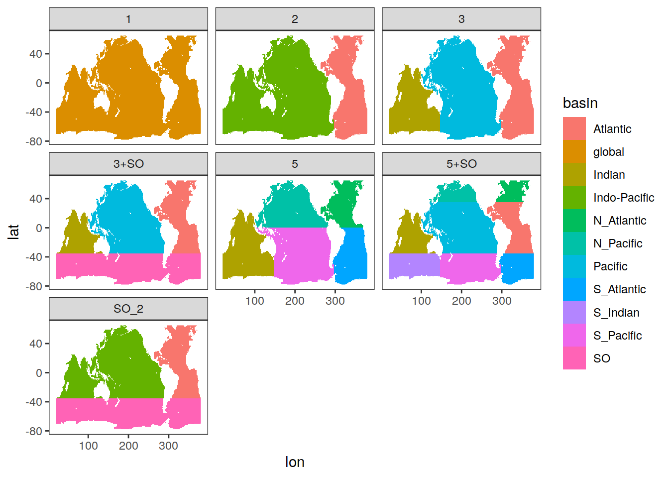
basinmask_all <- basinmask_all %>%
filter(MLR_basins != "SO_2")
basinmask_all %>% distinct(MLR_basins, basin)# A tibble: 23 × 2
basin MLR_basins
<chr> <chr>
1 global 1
2 Indo-Pacific 2
3 Atlantic 2
4 S_Pacific 5
5 S_Atlantic 5
6 Indian 5
7 N_Atlantic 5
8 N_Pacific 5
9 S_Pacific 5+SO
10 S_Atlantic 5+SO
# … with 13 more rowsbasinmask_all <- basinmask_all %>%
select(lon, lat, basin_mask = MLR_basins, basin_name = basin)
basinmask_all <- basinmask_all %>%
group_by(basin_mask) %>%
mutate(basin_name = as.numeric(as.factor(basin_name))) %>%
ungroup()
# convert from tibble to stars object
basinmask_all_out_stars <- st_as_stars(
basinmask_all,
dims = c(
"lon",
"lat",
"basin_mask"
)
)
# assign coordinate system to horizontal (lon, lat) coordinates
# st_crs(dcant_inv_out_stars) <- "+proj=longlat"
st_crs(basinmask_all_out_stars) <- st_crs(4326)
file_out <- paste0(path_out, "basin_mask_emlr_cstar_mueller_94-04-14.nc")
# write stars object to .nc file
basinmask_all_out_stars %>%
write_mdim(file_out)
# reopen .nc file with all available stars functions
basinmask_all_read_mdim <-
read_mdim(file_out)
# plot variable in object reopened
ggplot() +
geom_stars(data = basinmask_all_read_mdim,
aes(fill = as.factor(basin_name))) +
facet_wrap(~ basin_mask) +
scale_fill_muted(na.value = "transparent")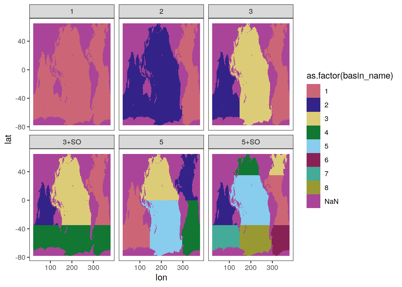
surface_area_mask <- basinmask_all %>%
filter(basin_mask == "1") %>%
select(-starts_with("basin")) %>%
mutate(surface_area = earth_surf(lat = lat, lon = lon))
surface_area_mask_out_stars <- st_as_stars(
surface_area_mask,
dims = c(
"lon",
"lat"
)
)
# assign coordinate system to horizontal (lon, lat) coordinates
# st_crs(dcant_inv_out_stars) <- "+proj=longlat"
st_crs(surface_area_mask_out_stars) <- st_crs(4326)
file_out <- paste0(path_out, "surface_area_mask_emlr_cstar_mueller_94-04-14.nc")
# write stars object to .nc file
surface_area_mask_out_stars %>%
write_mdim(file_out)21 Map test color palettes
breaks <- c(-Inf, seq(0, 16, 2), Inf)
legend_title <- expression(atop(Delta * C["ant"],
(mol ~ m ^ {
-2
})))
breaks_n <- length(breaks) - 1
dcant_inv_all_color_test <- dcant_inv_all %>%
filter(data_source %in% c("obs"),
period %in% two_decades) %>%
mutate(dcant_int = cut(dcant,
breaks,
right = FALSE))
scico_continous_palettes <- c(
"acton",
"bamako",
"batlow",
"bilbao",
"buda",
"davos",
"devon",
"grayC",
"hawaii",
"imola",
"lajolla",
"lapaz",
"nuuk",
"oslo",
"tokyo",
"turku"
)
p_test_scico <- function(df, i_palette) {
p_reg <- map +
geom_raster(data = df,
aes(lon, lat, fill = dcant_int)) +
scale_fill_scico_d(
palette = i_palette,
drop = FALSE,
name = legend_title,
guide = "none"
) +
labs(title = i_palette) +
theme(axis.text = element_blank(),
axis.ticks = element_blank()) +
facet_grid(.~period)
p_rev <- map +
geom_raster(data = df,
aes(lon, lat, fill = dcant_int)) +
scale_fill_scico_d(
palette = i_palette,
drop = FALSE,
name = legend_title,
direction = -1,
guide = "none"
) +
labs(title = paste(i_palette, "rev")) +
theme(axis.text = element_blank(),
axis.ticks = element_blank()) +
facet_grid(.~period)
p_comb <- p_reg / p_rev
return(p_comb)
}
all_plots_scico <- scico_continous_palettes %>%
# head(1) %>%
map(~p_test_scico(df = dcant_inv_all_color_test,
i_palette = .x))
viridis_continous_palettes <- c(
"viridis",
"magma",
"inferno",
"plasma"
)
p_test_viridis <- function(df, i_palette) {
p_reg <- map +
geom_raster(data = df,
aes(lon, lat, fill = dcant_int)) +
scale_fill_viridis_d(
option = i_palette,
drop = FALSE,
name = legend_title,
guide = "none"
) +
labs(title = i_palette) +
theme(axis.text = element_blank(),
axis.ticks = element_blank()) +
facet_grid(.~period)
p_rev <- map +
geom_raster(data = df,
aes(lon, lat, fill = dcant_int)) +
scale_fill_viridis_d(
option = i_palette,
drop = FALSE,
name = legend_title,
direction = -1,
guide = "none"
) +
labs(title = paste(i_palette, "rev")) +
theme(axis.text = element_blank(),
axis.ticks = element_blank()) +
facet_grid(.~period)
p_comb <- p_reg / p_rev
return(p_comb)
}
all_plots_viridis <- viridis_continous_palettes %>%
# head(1) %>%
map(~p_test_viridis(df = dcant_inv_all_color_test,
i_palette = .x))
library(colorspace)
colorspace_continous_palettes <- c(
# "Purple - Blue",
# "Red - Purple",
# "Blue - Yellow",
# "Heat",
# "Heat 2",
"Rocket"
# "Mako",
# "Dark",
# "Mint",
# "Mint",
# "BluGrn",
# "Teal",
# "Sunset",
# "SunsetDark",
# "ag_Sunset",
# "YlOrRd",
# "YlGnBu",
# "RdPu"
)
p_test_colorspace <- function(df, i_palette) {
i_palette <<- i_palette
p_reg <- map +
geom_raster(data = df,
aes(lon, lat, fill = dcant_int)) +
scale_fill_discrete_sequential(
palette = i_palette,
drop = FALSE,
name = legend_title,
guide = "none"
) +
labs(title = i_palette) +
theme(axis.text = element_blank(),
axis.ticks = element_blank()) +
facet_grid(.~period)
p_rev <- map +
geom_raster(data = df,
aes(lon, lat, fill = dcant_int)) +
scale_fill_discrete_sequential(
palette = i_palette,
drop = FALSE,
name = legend_title,
rev = FALSE,
guide = "none"
) +
labs(title = paste(i_palette, "rev")) +
theme(axis.text = element_blank(),
axis.ticks = element_blank()) +
facet_grid(.~period)
p_comb <- p_reg / p_rev
return(p_comb)
rm(i_palette)
}
all_plots_colorspace <- colorspace_continous_palettes %>%
# head(2) %>%
map(~p_test_colorspace(df = dcant_inv_all_color_test,
i_palette = .x))
all_plots_colorspace
all_plots <- c(all_plots_colorspace, all_plots_viridis, all_plots_scico)
pdf(here::here("output/publication/test_color_scales.pdf"),
width = 8, height = 4)
all_plots
dev.off()
sessionInfo()R version 4.2.2 (2022-10-31)
Platform: x86_64-pc-linux-gnu (64-bit)
Running under: openSUSE Leap 15.4
Matrix products: default
BLAS: /usr/local/R-4.2.2/lib64/R/lib/libRblas.so
LAPACK: /usr/local/R-4.2.2/lib64/R/lib/libRlapack.so
locale:
[1] LC_CTYPE=en_US.UTF-8 LC_NUMERIC=C
[3] LC_TIME=en_US.UTF-8 LC_COLLATE=en_US.UTF-8
[5] LC_MONETARY=en_US.UTF-8 LC_MESSAGES=en_US.UTF-8
[7] LC_PAPER=en_US.UTF-8 LC_NAME=C
[9] LC_ADDRESS=C LC_TELEPHONE=C
[11] LC_MEASUREMENT=en_US.UTF-8 LC_IDENTIFICATION=C
attached base packages:
[1] stats graphics grDevices utils datasets methods base
other attached packages:
[1] rqdatatable_1.3.1 rquery_1.4.9 wrapr_2.0.9
[4] stars_0.6-0 abind_1.4-5 ggpattern_1.0.1
[7] ggh4x_0.2.3 khroma_1.9.0 kableExtra_1.3.4
[10] ggdist_3.2.0 ggalluvial_0.12.3 terra_1.6-41
[13] sf_1.0-9 rnaturalearth_0.1.0 geomtextpath_0.1.1
[16] colorspace_2.0-3 marelac_2.1.10 shape_1.4.6
[19] ggforce_0.4.1 metR_0.13.0 scico_1.3.1
[22] patchwork_1.1.2 collapse_1.8.9 forcats_0.5.2
[25] stringr_1.4.1 dplyr_1.0.10 purrr_0.3.5
[28] readr_2.1.3 tidyr_1.2.1 tibble_3.1.8
[31] ggplot2_3.4.0 tidyverse_1.3.2 workflowr_1.7.0
loaded via a namespace (and not attached):
[1] readxl_1.4.1 backports_1.4.1 systemfonts_1.0.4
[4] lwgeom_0.2-10 plyr_1.8.8 splines_4.2.2
[7] sp_1.5-1 digest_0.6.30 htmltools_0.5.3
[10] fansi_1.0.3 magrittr_2.0.3 checkmate_2.1.0
[13] memoise_2.0.1 googlesheets4_1.0.1 tzdb_0.3.0
[16] modelr_0.1.10 vroom_1.6.0 svglite_2.1.0
[19] timechange_0.1.1 rvest_1.0.3 textshaping_0.3.6
[22] haven_2.5.1 xfun_0.35 callr_3.7.3
[25] crayon_1.5.2 jsonlite_1.8.3 zoo_1.8-11
[28] glue_1.6.2 polyclip_1.10-4 gtable_0.3.1
[31] gargle_1.2.1 webshot_0.5.4 distributional_0.3.1
[34] scales_1.2.1 DBI_1.1.3 Rcpp_1.0.9
[37] isoband_0.2.6 viridisLite_0.4.1 units_0.8-0
[40] bit_4.0.5 proxy_0.4-27 httr_1.4.4
[43] seacarb_3.3.1 RColorBrewer_1.1-3 ellipsis_0.3.2
[46] pkgconfig_2.0.3 farver_2.1.1 sass_0.4.4
[49] dbplyr_2.2.1 utf8_1.2.2 here_1.0.1
[52] tidyselect_1.2.0 labeling_0.4.2 rlang_1.0.6
[55] later_1.3.0 munsell_0.5.0 cellranger_1.1.0
[58] tools_4.2.2 cachem_1.0.6 cli_3.4.1
[61] generics_0.1.3 broom_1.0.1 evaluate_0.18
[64] fastmap_1.1.0 yaml_2.3.6 ragg_1.2.4
[67] oce_1.7-10 processx_3.8.0 knitr_1.41
[70] bit64_4.0.5 fs_1.5.2 nlme_3.1-160
[73] whisker_0.4 xml2_1.3.3 compiler_4.2.2
[76] rstudioapi_0.14 e1071_1.7-12 reprex_2.0.2
[79] tweenr_2.0.2 bslib_0.4.1 stringi_1.7.8
[82] highr_0.9 ps_1.7.2 lattice_0.20-45
[85] Matrix_1.5-3 classInt_0.4-8 vctrs_0.5.1
[88] pillar_1.8.1 lifecycle_1.0.3 jquerylib_0.1.4
[91] gsw_1.1-1 data.table_1.14.6 httpuv_1.6.6
[94] R6_2.5.1 promises_1.2.0.1 KernSmooth_2.23-20
[97] codetools_0.2-18 MASS_7.3-58.1 assertthat_0.2.1
[100] rprojroot_2.0.3 withr_2.5.0 SolveSAPHE_2.1.0
[103] mgcv_1.8-41 parallel_4.2.2 hms_1.1.2
[106] grid_4.2.2 rnaturalearthdata_0.1.0 class_7.3-20
[109] rmarkdown_2.18 googledrive_2.0.0 git2r_0.30.1
[112] getPass_0.2-2 lubridate_1.9.0