CMEMS
Jens Daniel Müller
16 May, 2024
Last updated: 2024-05-16
Checks: 7 0
Knit directory:
heatwave_co2_flux_2023/analysis/
This reproducible R Markdown analysis was created with workflowr (version 1.7.0). The Checks tab describes the reproducibility checks that were applied when the results were created. The Past versions tab lists the development history.
Great! Since the R Markdown file has been committed to the Git repository, you know the exact version of the code that produced these results.
Great job! The global environment was empty. Objects defined in the global environment can affect the analysis in your R Markdown file in unknown ways. For reproduciblity it’s best to always run the code in an empty environment.
The command set.seed(20240307) was run prior to running
the code in the R Markdown file. Setting a seed ensures that any results
that rely on randomness, e.g. subsampling or permutations, are
reproducible.
Great job! Recording the operating system, R version, and package versions is critical for reproducibility.
Nice! There were no cached chunks for this analysis, so you can be confident that you successfully produced the results during this run.
Great job! Using relative paths to the files within your workflowr project makes it easier to run your code on other machines.
Great! You are using Git for version control. Tracking code development and connecting the code version to the results is critical for reproducibility.
The results in this page were generated with repository version 3f7c586. See the Past versions tab to see a history of the changes made to the R Markdown and HTML files.
Note that you need to be careful to ensure that all relevant files for
the analysis have been committed to Git prior to generating the results
(you can use wflow_publish or
wflow_git_commit). workflowr only checks the R Markdown
file, but you know if there are other scripts or data files that it
depends on. Below is the status of the Git repository when the results
were generated:
Ignored files:
    Ignored:    .Rhistory
    Ignored:    .Rproj.user/
    Ignored:    data/

Unstaged changes:
    Modified:   analysis/child/pCO2_product_synopsis.Rmd
    Modified:   code/Workflowr_project_managment.R
Note that any generated files, e.g. HTML, png, CSS, etc., are not included in this status report because it is ok for generated content to have uncommitted changes.
These are the previous versions of the repository in which changes were
made to the R Markdown (analysis/CMEMS.Rmd) and HTML
(docs/CMEMS.html) files. If you’ve configured a remote Git
repository (see ?wflow_git_remote), click on the hyperlinks
in the table below to view the files as they were in that past version.
| File | Version | Author | Date | Message |
|---|---|---|---|---|
| Rmd | 3f7c586 | jens-daniel-mueller | 2024-05-16 | CMEMS sfco2 data included |
| html | 51df30d | jens-daniel-mueller | 2024-05-15 | Build site. |
| Rmd | 981d5e1 | jens-daniel-mueller | 2024-05-15 | kw K0 product included, mean flux densities computed |
| html | 009791f | jens-daniel-mueller | 2024-05-14 | Build site. |
| html | 3b5d16b | jens-daniel-mueller | 2024-05-13 | Build site. |
| Rmd | 1e1dee5 | jens-daniel-mueller | 2024-05-13 | pco2 to fco2 conversions, changed output files |
| html | 77accd5 | jens-daniel-mueller | 2024-05-07 | Build site. |
| Rmd | e5f46df | jens-daniel-mueller | 2024-05-07 | new input files, revised date format and temperature scale |
| html | e9c4ecf | jens-daniel-mueller | 2024-05-07 | Build site. |
| Rmd | b9670ef | jens-daniel-mueller | 2024-05-07 | new input files, revised date format |
| Rmd | e17c3fc | jens-daniel-mueller | 2024-05-07 | manual commit |
| html | 5d10d21 | jens-daniel-mueller | 2024-05-07 | Build site. |
| Rmd | 14c0b11 | jens-daniel-mueller | 2024-05-07 | new input files |
| html | 7f9c687 | jens-daniel-mueller | 2024-04-23 | Build site. |
| html | ce4e2a6 | jens-daniel-mueller | 2024-04-17 | Build site. |
| html | 58e3680 | jens-daniel-mueller | 2024-04-11 | Build site. |
| html | dfcf790 | jens-daniel-mueller | 2024-04-11 | Build site. |
| html | 139bc97 | jens-daniel-mueller | 2024-04-11 | manual deletion of files |
| html | 2321242 | jens-daniel-mueller | 2024-04-11 | Build site. |
| Rmd | d98842b | jens-daniel-mueller | 2024-04-10 | fixed anomaly year output |
| html | 07ccdb0 | jens-daniel-mueller | 2024-04-05 | Build site. |
| Rmd | ad6839e | jens-daniel-mueller | 2024-04-05 | fixed anomaly maps |
| html | 69dc18c | jens-daniel-mueller | 2024-04-04 | Build site. |
| html | c9d994c | jens-daniel-mueller | 2024-04-04 | Build site. |
| Rmd | 46f044d | jens-daniel-mueller | 2024-04-04 | rebuild entire website with individual anomaly years |
| Rmd | 9d258b5 | jens-daniel-mueller | 2024-04-03 | manual commit |
| html | 6bb7ce2 | jens-daniel-mueller | 2024-03-25 | Build site. |
| html | f9d2b99 | jens-daniel-mueller | 2024-03-25 | total cummulative intensity added |
| html | 3114859 | jens-daniel-mueller | 2024-03-25 | Build site. |
| html | 4589270 | jens-daniel-mueller | 2024-03-24 | Build site. |
| Rmd | 78b2c56 | jens-daniel-mueller | 2024-03-24 | new figure aspect ratios |
| html | 5c1676b | jens-daniel-mueller | 2024-03-24 | Build site. |
| Rmd | 31ffcb9 | jens-daniel-mueller | 2024-03-24 | CMEMS unit error fixed |
| html | a1c2e14 | jens-daniel-mueller | 2024-03-24 | Build site. |
| Rmd | c32eb8f | jens-daniel-mueller | 2024-03-24 | CMEMS analysis |
| html | 62ea4dd | jens-daniel-mueller | 2024-03-24 | Build site. |
| html | 1a5167d | jens-daniel-mueller | 2024-03-24 | Build site. |
| Rmd | cf4f62f | jens-daniel-mueller | 2024-03-23 | MHW stats and CMEMS added |
center <- -160
boundary <- center + 180
target_crs <- paste0("+proj=robin +over +lon_0=", center)
# target_crs <- paste0("+proj=eqearth +over +lon_0=", center)
# target_crs <- paste0("+proj=eqearth +lon_0=", center)
# target_crs <- paste0("+proj=igh_o +lon_0=", center)

worldmap <- ne_countries(scale = 'small',
                         type = 'map_units',
                         returnclass = 'sf')

worldmap <- worldmap %>% st_break_antimeridian(lon_0 = center)
worldmap_trans <- st_transform(worldmap, crs = target_crs)

# ggplot() +
#   geom_sf(data = worldmap_trans)

coastline <- ne_coastline(scale = 'small', returnclass = "sf")
coastline <- st_break_antimeridian(coastline, lon_0 = 200)
coastline_trans <- st_transform(coastline, crs = target_crs)

# ggplot() +
#   geom_sf(data = worldmap_trans, fill = "grey", col="grey") +
#   geom_sf(data = coastline_trans)


bbox <- st_bbox(c(xmin = -180, xmax = 180, ymax = 65, ymin = -78), crs = st_crs(4326))
bbox <- st_as_sfc(bbox)
bbox_trans <- st_break_antimeridian(bbox, lon_0 = center)

bbox_graticules <- st_graticule(
  x = bbox_trans,
  crs = st_crs(bbox_trans),
  datum = st_crs(bbox_trans),
  lon = c(20, 20.001),
  lat = c(-78,65),
  ndiscr = 1e3,
  margin = 0.001
)

bbox_graticules_trans <- st_transform(bbox_graticules, crs = target_crs)
rm(worldmap, coastline, bbox, bbox_trans)

# ggplot() +
#   geom_sf(data = worldmap_trans, fill = "grey", col="grey") +
#   geom_sf(data = coastline_trans) +
#   geom_sf(data = bbox_graticules_trans)

lat_lim <- ext(bbox_graticules_trans)[c(3,4)]*1.002
lon_lim <- ext(bbox_graticules_trans)[c(1,2)]*1.005

# ggplot() +
#   geom_sf(data = worldmap_trans, fill = "grey90", col = "grey90") +
#   geom_sf(data = coastline_trans) +
#   geom_sf(data = bbox_graticules_trans, linewidth = 1) +
#   coord_sf(crs = target_crs,
#            ylim = lat_lim,
#            xlim = lon_lim,
#            expand = FALSE) +
#   theme(
#     panel.border = element_blank(),
#     axis.text = element_blank(),
#     axis.ticks = element_blank()
#   )

latitude_graticules <- st_graticule(
  x = bbox_graticules,
  crs = st_crs(bbox_graticules),
  datum = st_crs(bbox_graticules),
  lon = c(20, 20.001),
  lat = c(-60,-30,0,30,60),
  ndiscr = 1e3,
  margin = 0.001
)

latitude_graticules_trans <- st_transform(latitude_graticules, crs = target_crs)

latitude_labels <- data.frame(lat_label = c("60°N","30°N","Eq.","30°S","60°S"),
                 lat = c(60,30,0,-30,-60)-4, lon = c(35)-c(0,2,4,2,0))

latitude_labels <- st_as_sf(x = latitude_labels,
               coords = c("lon", "lat"),
               crs = "+proj=longlat")

latitude_labels_trans <- st_transform(latitude_labels, crs = target_crs)

# ggplot() +
#   geom_sf(data = worldmap_trans, fill = "grey", col = "grey") +
#   geom_sf(data = coastline_trans) +
#   geom_sf(data = bbox_graticules_trans) +
#   geom_sf(data = latitude_graticules_trans,
#           col = "grey60",
#           linewidth = 0.2) +
#   geom_sf_text(data = latitude_labels_trans,
#                aes(label = lat_label),
#                size = 3,
#                col = "grey60")
Read data
path_pCO2_products <-
  "/nfs/kryo/work/datasets/gridded/ocean/2d/observation/pco2/"

path_CMEMS <- paste0(path_pCO2_products, "cmems_ffnn/v2023/r100_regridded/")
library(ncdf4)
nc <-
nc_open(paste0(
path_pCO2_products,
"VLIZ-SOM_FFN/VLIZ-SOM_FFN_vBAMS2024.nc"
))
nc <-
nc_open(paste0(
path_CMEMS,
"kw_OceanSODA_ETHZ_HR_LR-v2023.01-1982_2023.nc"
))
nc <-
nc_open(paste0(
path_CMEMS,
"CO2_fluxes/fluxCO2_model_v2022_r100_202402.nc"
))
nc <-
nc_open(paste0(
path_CMEMS,
"SSH_r100_199205.nc"
))
nc <-
nc_open("/nfs/kryo/work/datasets/gridded/ocean/2d/observation/pco2/cmems_ffnn/v2020/v2020.nc")
print(nc)
ncatt_get(nc, varid = "time")
ncvar_get(nc, varid = "time")CMEMS_files <- list.files(path = path_CMEMS)
CMEMS_files <- CMEMS_files[!(CMEMS_files %>% str_detect("fuCO2_clim"))]
# CMEMS_files <- str_remove(CMEMS_files, ".nc")
# CMEMS_files_dates <- str_sub(CMEMS_files, start = -6)
# CMEMS_files_names <- str_sub(CMEMS_files, end = -8)
# CMEMS_files_names <- str_remove(CMEMS_files_names, "_r100")
# CMEMS_files <- bind_cols(file_name_variable = CMEMS_files_names, file_name_date = CMEMS_files_dates)
# library(lubridate)
# CMEMS_files <- CMEMS_files %>%
# mutate(date = ym(file_name_date))
# CMEMS_files %>%
# filter(year(date) >= 2023) %>%
# ggplot(aes(file_name_date, file_name_variable)) +
# geom_point()
CMEMS_files <- CMEMS_files[!(CMEMS_files %>% str_detect("UV"))]
CMEMS_files <- CMEMS_files[!(CMEMS_files %>% str_detect("Ps"))]
CMEMS_files <- CMEMS_files[!(CMEMS_files %>% str_detect("Sea_Ice"))]
# print(CMEMS_files, max = 5000)
file_names <- str_split(CMEMS_files, "_", simplify = TRUE)[,1] %>% unique()
for (i_file_name in file_names) {
# i_file_name <- file_names[3]
CMEMS_files_var <-
CMEMS_files[CMEMS_files %>% str_detect(i_file_name)]
if(i_file_name == "xCO2"){
CMEMS_files_var <-
CMEMS_files_var[!CMEMS_files_var %>% str_detect("fluxCO2")]
}
for (i_name in CMEMS_files_var) {
# i_name <- CMEMS_files_var[465]
# i_name <- CMEMS_files_var[466]
# print(i_name)
library(ncdf4)
nc <- nc_open(paste0(path_CMEMS, i_name))
var_name <- names(nc$var)[1]
i_pco2_product_var <-
read_ncdf(paste0(path_CMEMS, i_name),
make_units = FALSE,
var = var_name)
if (exists("pco2_product_var")) {
pco2_product_var <-
c(pco2_product_var,
i_pco2_product_var)
}
if (!exists("pco2_product_var")) {
pco2_product_var <- i_pco2_product_var
}
# ggplot() +
# geom_stars(data = pco2_product_var) +
# scale_fill_viridis_c(trans = "log10", na.value = "red") +
# facet_wrap(~ time)
}
pco2_product_var <- pco2_product_var %>%
as_tibble()
pco2_product_var <-
pco2_product_var %>%
mutate(
area = earth_surf(lat, lon),
year = year(time),
month = month(time),
time = ymd(paste(year, month, "15", sep = "-"))
)
# ggplot() +
# geom_raster(data = pco2_product_var, aes(lon, lat, fill = CHL)) +
# scale_fill_viridis_c(trans = "log10", na.value = "red") +
# facet_wrap( ~ time)
if (exists("pco2_product")) {
pco2_product <-
full_join(pco2_product,
pco2_product_var)
}
if (!exists("pco2_product")) {
pco2_product <- pco2_product_var
}
rm(pco2_product_var)
}
rm(i_pco2_product_var,
nc, var_name,
i_file_name, file_names,
i_name, CMEMS_files_var,
CMEMS_files)
# rm(pco2_product)
pco2_product <-
pco2_product %>%
rename(chl = CHL,
mld = MLD,
atm_co2 = CO2,
fgco2 = fCO2_mean,
sfco2 = fuCO2_mean,
salinity = SSS,
temperature = SST)
pco2_product <-
pco2_product %>%
mutate(lon = if_else(lon < 20, lon + 360, lon),
fgco2 = -fgco2,
chl = log10(chl),
mld = log10(mld))
pco2_product <-
pco2_product %>%
mutate(temperature = if_else(
year == 2023 & month >=10,
temperature - 273.15,
temperature
))
# ggplot() +
# geom_raster(data = pco2_product %>%
# filter(year == 2023,
# month %in% 9:10),
# aes(lon, lat, fill = chl)) +
# scale_fill_viridis_c(na.value = "red") +
# facet_wrap( ~ month)
pco2_product <-
pco2_product %>%
filter(year <= 2023)
pco2_product <-
pco2_product %>%
mutate(
atm_fco2 = p2fCO2(T = temperature,
pCO2 = atm_co2),
dfco2 = sfco2 - atm_fco2
)
pco2_product <-
pco2_product %>%
select(-c(atm_co2))
# pco2_product <-
# pco2_product %>%
# mutate(kw_sol = kw * sol)names <- c("CO2_fluxes", "CO2_fugacity")
for (i_name in names) {
# i_name <- names[2]
CMEMS_files <- list.files(path = paste0(path_CMEMS, i_name, "/"),
full.names = TRUE)
# i_CMEMS_files <- CMEMS_files[2]
i_pco2_product <-
read_stars(CMEMS_files,
make_units = FALSE,
ignore_bounds = TRUE,
quiet = TRUE)
if (exists("pco2_product")) {
pco2_product <-
c(pco2_product,
i_pco2_product)
}
if (!exists("pco2_product")) {
pco2_product <- i_pco2_product
}
}
rm(CMEMS_files, i_pco2_product, i_name, names)
# rm(pco2_product)
pco2_product <- pco2_product %>%
as_tibble()
pco2_product <-
pco2_product %>%
rename(lon = x,
lat = y,
sfco2 = fuCO2_mean,
fgco2 = fCO2_mean) %>%
select(-contains("_std")) %>%
units::drop_units()
pco2_product <-
pco2_product %>%
mutate(area = earth_surf(lat, lon),
year = year(time),
month = month(time))
pco2_product <-
pco2_product %>%
mutate(lon = if_else(lon < 20, lon + 360, lon),
fgco2 = -fgco2)
pco2_product <-
pco2_product %>%
filter(year <= 2023)pCO2_product_preprocessing <-
knitr::knit_expand(file = here::here("analysis/child/pCO2_product_preprocessing.Rmd"))Preprocessing
Load masks
biome_mask <-
  read_rds(here::here("data/biome_mask.rds"))

map <-
  read_rds(here::here("data/map.rds"))

key_biomes <-
  read_rds(here::here("data/key_biomes.rds"))

super_biomes <-
  read_rds(here::here("data/super_biomes.rds"))

super_biome_mask <-
  read_rds(here::here("data/super_biome_mask.rds"))
Define labels and breaks
labels_breaks <- function(i_name) {

  if (i_name == "dco2") {
    i_legend_title <- "ΔpCO<sub>2</sub><br>(µatm)"
    # i_breaks <- c(-Inf, seq(0, 80, 10), Inf)
    # i_contour_level <- 50
    # i_contour_level_abs <- 2200
  }

  if (i_name == "dfco2") {
    i_legend_title <- "ΔfCO<sub>2</sub><br>(µatm)"
    # i_breaks <- c(-Inf, seq(0, 80, 10), Inf)
    # i_contour_level <- 50
    # i_contour_level_abs <- 2200
  }

  if (i_name == "atm_co2") {
    i_legend_title <- "pCO<sub>2,atm</sub><br>(µatm)"
    # i_breaks <- c(-Inf, seq(0, 80, 10), Inf)
    # i_contour_level <- 50
    # i_contour_level_abs <- 2200
  }

  if (i_name == "atm_fco2") {
    i_legend_title <- "fCO<sub>2,atm</sub><br>(µatm)"
    # i_breaks <- c(-Inf, seq(0, 80, 10), Inf)
    # i_contour_level <- 50
    # i_contour_level_abs <- 2200
  }

  if (i_name == "sol") {
    i_legend_title <- "K<sub>0</sub><br>(mol m<sup>-3</sup> µatm<sup>-1</sup>)"
    # i_breaks <- c(-Inf, seq(0, 80, 10), Inf)
    # i_contour_level <- 50
    # i_contour_level_abs <- 2200
  }

  if (i_name == "kw") {
    i_legend_title <- "k<sub>w</sub><br>(m yr<sup>-1</sup>)"
    # i_breaks <- c(-Inf, seq(0, 80, 10), Inf)
    # i_contour_level <- 50
    # i_contour_level_abs <- 2200
  }

  if (i_name == "kw_sol") {
    i_legend_title <- "k<sub>w</sub> K<sub>0</sub><br>(mol yr<sup>-1</sup> m<sup>-2</sup> µatm<sup>-1</sup>)"
    # i_breaks <- c(-Inf, seq(0, 80, 10), Inf)
    # i_contour_level <- 50
    # i_contour_level_abs <- 2200
  }

  if (i_name == "spco2") {
    i_legend_title <- "pCO<sub>2,ocean</sub><br>(µatm)"
    # i_breaks <- c(-Inf, seq(0, 80, 10), Inf)
    # i_contour_level <- 50
    # i_contour_level_abs <- 2200
  }

  if (i_name == "sfco2") {
    i_legend_title <- "fCO<sub>2,ocean</sub><br>(µatm)"
    # i_breaks <- c(-Inf, seq(0, 80, 10), Inf)
    # i_contour_level <- 50
    # i_contour_level_abs <- 2200
  }

  if (i_name == "fgco2") {
    i_legend_title <- "FCO<sub>2</sub><br>(mol m<sup>-2</sup> yr<sup>-1</sup>)"
    # i_breaks <- c(-Inf, seq(0, 80, 10), Inf)
    # i_contour_level <- 50
    # i_contour_level_abs <- 2200
  }

  if (i_name == "fgco2_hov") {
    i_legend_title <- "FCO<sub>2</sub><br>(PgC deg<sup>-1</sup> yr<sup>-1</sup>)"
    # i_breaks <- c(-Inf, seq(0, 80, 10), Inf)
    # i_contour_level <- 50
    # i_contour_level_abs <- 2200
  }

  if (i_name == "fgco2_int") {
    i_legend_title <- "FCO<sub>2</sub><br>(PgC yr<sup>-1</sup>)"
    # i_breaks <- c(-Inf, seq(0, 80, 10), Inf)
    # i_contour_level <- 50
    # i_contour_level_abs <- 2200
  }

  if (i_name == "temperature") {
    i_legend_title <- "SST<br>(°C)"
    # i_breaks <- c(-Inf, seq(0, 80, 10), Inf)
    # i_contour_level <- 50
    # i_contour_level_abs <- 2200
  }

  if (i_name == "salinity") {
    i_legend_title <- "SSS"
    # i_breaks <- c(-Inf, seq(0, 80, 10), Inf)
    # i_contour_level <- 50
    # i_contour_level_abs <- 2200
  }

  if (i_name == "chl") {
    i_legend_title <- "lg(Chl-a)<br>(lg(mg m<sup>-3</sup>))"
    # i_breaks <- c(-Inf, seq(0, 80, 10), Inf)
    # i_contour_level <- 50
    # i_contour_level_abs <- 2200
  }

  if (i_name == "mld") {
    i_legend_title <- "lg(MLD)<br>(lg(m))"
    # i_breaks <- c(-Inf, seq(0, 80, 10), Inf)
    # i_contour_level <- 50
    # i_contour_level_abs <- 2200
  }

  if (i_name == "press") {
    i_legend_title <- "pressure<sub>atm</sub><br>(Pa)"
    # i_breaks <- c(-Inf, seq(0, 80, 10), Inf)
    # i_contour_level <- 50
    # i_contour_level_abs <- 2200
  }

  if (i_name == "wind") {
    i_legend_title <- "Wind <br>(m sec<sup>-1</sup>)"
    # i_breaks <- c(-Inf, seq(0, 80, 10), Inf)
    # i_contour_level <- 50
    # i_contour_level_abs <- 2200
  }

  if (i_name == "SSH") {
    i_legend_title <- "SSH <br>(m)"
    # i_breaks <- c(-Inf, seq(0, 80, 10), Inf)
    # i_contour_level <- 50
    # i_contour_level_abs <- 2200
  }

  if (i_name == "fice") {
    i_legend_title <- "Sea ice <br>(%)"
    # i_breaks <- c(-Inf, seq(0, 80, 10), Inf)
    # i_contour_level <- 50
    # i_contour_level_abs <- 2200
  }

  all_labels_breaks <- lst(i_legend_title,
                           # i_breaks,
                           # i_contour_level,
                           # i_contour_level_abs
                           )

  return(all_labels_breaks)

}


# labels_breaks("fgco2")

x_axis_labels <-
  c(
    "dco2" = labels_breaks("dco2")$i_legend_title,
    "dfco2" = labels_breaks("dfco2")$i_legend_title,
    "atm_co2" = labels_breaks("atm_co2")$i_legend_title,
    "atm_fco2" = labels_breaks("atm_fco2")$i_legend_title,
    "sol" = labels_breaks("sol")$i_legend_title,
    "kw" = labels_breaks("kw")$i_legend_title,
    "kw_sol" = labels_breaks("kw_sol")$i_legend_title,
    "spco2" = labels_breaks("spco2")$i_legend_title,
    "sfco2" = labels_breaks("sfco2")$i_legend_title,
    "fgco2" = labels_breaks("fgco2")$i_legend_title,
    "fgco2_hov" = labels_breaks("fgco2_hov")$i_legend_title,
    "fgco2_int" = labels_breaks("fgco2_int")$i_legend_title,
    "temperature" = labels_breaks("temperature")$i_legend_title,
    "salinity" = labels_breaks("salinity")$i_legend_title,
    "chl" = labels_breaks("chl")$i_legend_title,
    "mld" = labels_breaks("mld")$i_legend_title,
    "press" = labels_breaks("press")$i_legend_title,
    "wind" = labels_breaks("wind")$i_legend_title,
    "SSH" = labels_breaks("SSH")$i_legend_title,
    "fice" = labels_breaks("fice")$i_legend_title
  )
Analysis settings
name_quadratic_fit <- c("atm_co2", "atm_fco2", "spco2", "sfco2")

start_year <- 1990

name_divergent <- c("dco2", "dfco2", "fgco2", "fgco2_hov", "fgco2_int")
Data preprocessing
pco2_product <-
  pco2_product %>%
  filter(year >= start_year)
pco2_product <-
full_join(pco2_product,
biome_mask)
# set all values outside biome mask to NA
pco2_product <-
pco2_product %>%
mutate(across(-c(lat, lon, time, area, year, month, biome),
~ if_else(is.na(biome), NA, .)))Compuations
# apply coarse grid

pco2_product_coarse <-
  m_grid_horizontal_coarse(pco2_product)

pco2_product_coarse <-
  pco2_product_coarse %>%
  select(-c(lon, lat, time, biome)) %>%
  group_by(year, month, lon_grid, lat_grid) %>%
  summarise(across(-area,
                   ~ weighted.mean(., area))) %>%
  ungroup() %>%
  rename(lon = lon_grid, lat = lat_grid)

pco2_product_coarse <-
  pco2_product_coarse %>%
  pivot_longer(-c(year, month, lon, lat)) %>%
  drop_na() %>%
  pivot_wider()

# compute annual means

pco2_product_coarse_annual <-
  pco2_product_coarse %>%
  select(-month) %>%
  group_by(year, lon, lat) %>%
  summarise(across(where(is.numeric),
                   ~ mean(.))) %>%
  ungroup()

pco2_product_coarse_annual <-
  pco2_product_coarse_annual %>%
  pivot_longer(-c(year, lon, lat))

## compute monthly means

pco2_product_coarse_monthly <-
  pco2_product_coarse %>%
  group_by(year, month, lon, lat) %>%
  summarise(across(where(is.numeric),
                   ~ mean(.))) %>%
  ungroup()

pco2_product_coarse_monthly <-
  pco2_product_coarse_monthly %>%
  pivot_longer(-c(year, month, lon, lat))
pco2_product_monthly_global <-
pco2_product %>%
filter(!is.na(fgco2)) %>%
mutate(fgco2_int = fgco2) %>%
select(-c(lon, lat, year, month, biome)) %>%
group_by(time) %>%
summarise(across(-c(fgco2_int, area),
~ weighted.mean(., area, na.rm = TRUE)),
across(fgco2_int,
~ sum(. * area, na.rm = TRUE) * 12.01 * 1e-15)) %>%
ungroup()
pco2_product_monthly_biome <-
pco2_product %>%
filter(!is.na(fgco2)) %>%
mutate(fgco2_int = fgco2) %>%
select(-c(lon, lat, year, month)) %>%
group_by(time, biome) %>%
summarise(across(-c(fgco2_int, area),
~ weighted.mean(., area, na.rm = TRUE)),
across(fgco2_int,
~ sum(. * area, na.rm = TRUE) * 12.01 * 1e-15)) %>%
ungroup()
pco2_product_monthly_biome_super <-
pco2_product %>%
filter(!is.na(fgco2)) %>%
mutate(fgco2_int = fgco2) %>%
mutate(
biome = case_when(
str_detect(biome, "NA-") ~ "North Atlantic",
str_detect(biome, "NP-") ~ "North Pacific",
str_detect(biome, "SO-") ~ "Southern Ocean",
TRUE ~ "other"
)
) %>%
filter(biome != "other") %>%
select(-c(lon, lat, year, month)) %>%
group_by(time, biome) %>%
summarise(across(-c(fgco2_int, area),
~ weighted.mean(., area, na.rm = TRUE)),
across(fgco2_int,
~ sum(. * area, na.rm = TRUE) * 12.01 * 1e-15)) %>%
ungroup()
pco2_product_monthly <-
bind_rows(pco2_product_monthly_global %>%
mutate(biome = "Global"),
pco2_product_monthly_biome,
pco2_product_monthly_biome_super)
rm(
pco2_product_monthly_global,
pco2_product_monthly_biome,
pco2_product_monthly_biome_super
)
pco2_product_monthly <-
pco2_product_monthly %>%
filter(!is.na(biome))
pco2_product_monthly <-
pco2_product_monthly %>%
mutate(year = year(time),
month = month(time),
.after = time)
pco2_product_monthly <-
pco2_product_monthly %>%
pivot_longer(-c(time, year, month, biome))Absolute values
Hovmoeller plots
The following Hovmoeller plots show the value of each variable as provided through the pCO2 product. Hovmoeller plots are first presented as annual means, and than as monthly means.
Annual means
pco2_product_hovmoeller_monthly_annual <-
  pco2_product %>%
  mutate(fgco2_int = fgco2) %>%
  select(-c(lon, time, month, biome)) %>%
  group_by(year, lat) %>%
  summarise(across(-c(fgco2_int, area),
                   ~ weighted.mean(., area, na.rm = TRUE)),
            across(fgco2_int,
                   ~ sum(. * area, na.rm = TRUE) * 12.01 * 1e-15)) %>%
  ungroup() %>%
  rename(fgco2_hov = fgco2_int) %>%
  filter(fgco2_hov != 0)

pco2_product_hovmoeller_monthly_annual <-
  pco2_product_hovmoeller_monthly_annual %>%
  pivot_longer(-c(year, lat)) %>%
  drop_na()

pco2_product_hovmoeller_monthly_annual %>%
  filter(!(name %in% name_divergent)) %>%
  group_split(name) %>%
  # tail(5) %>%
  map(
    ~ ggplot(data = .x,
             aes(year, lat, fill = value)) +
      geom_raster() +
      scale_fill_viridis_c(name = labels_breaks(.x %>% distinct(name))) +
      theme(legend.title = element_markdown()) +
      coord_cartesian(expand = 0) +
      labs(title = "Annual means",
           y = "Latitude") +
      theme(axis.title.x = element_blank())
  )
[[1]]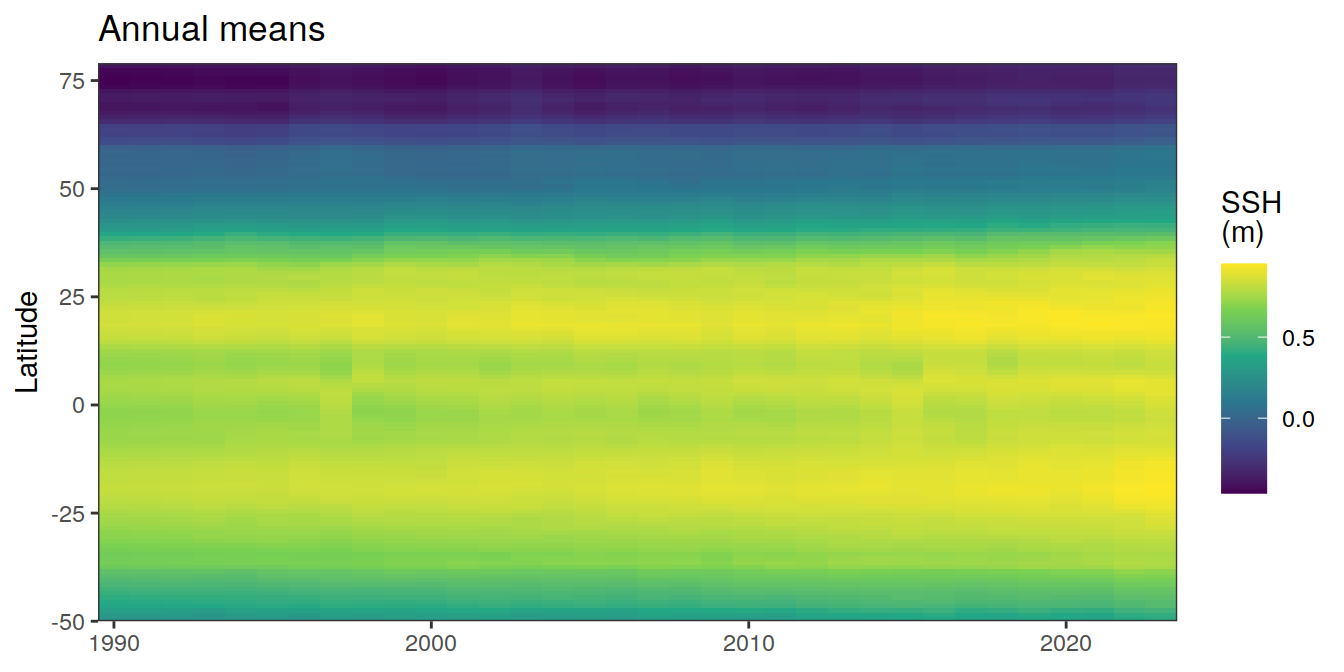
[[2]]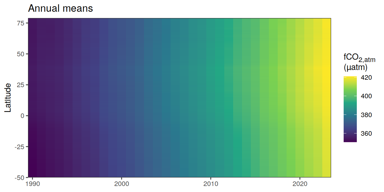
| Version | Author | Date |
|---|---|---|
| 009791f | jens-daniel-mueller | 2024-05-14 |
| 3b5d16b | jens-daniel-mueller | 2024-05-13 |
| e9c4ecf | jens-daniel-mueller | 2024-05-07 |
| 5d10d21 | jens-daniel-mueller | 2024-05-07 |
| dfcf790 | jens-daniel-mueller | 2024-04-11 |
| 89becff | jens-daniel-mueller | 2024-04-11 |
| 5c1676b | jens-daniel-mueller | 2024-03-24 |
| a1c2e14 | jens-daniel-mueller | 2024-03-24 |
[[3]]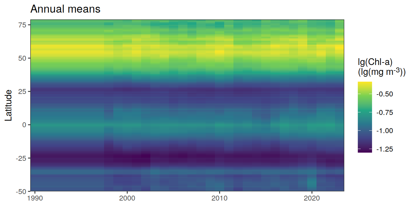
[[4]]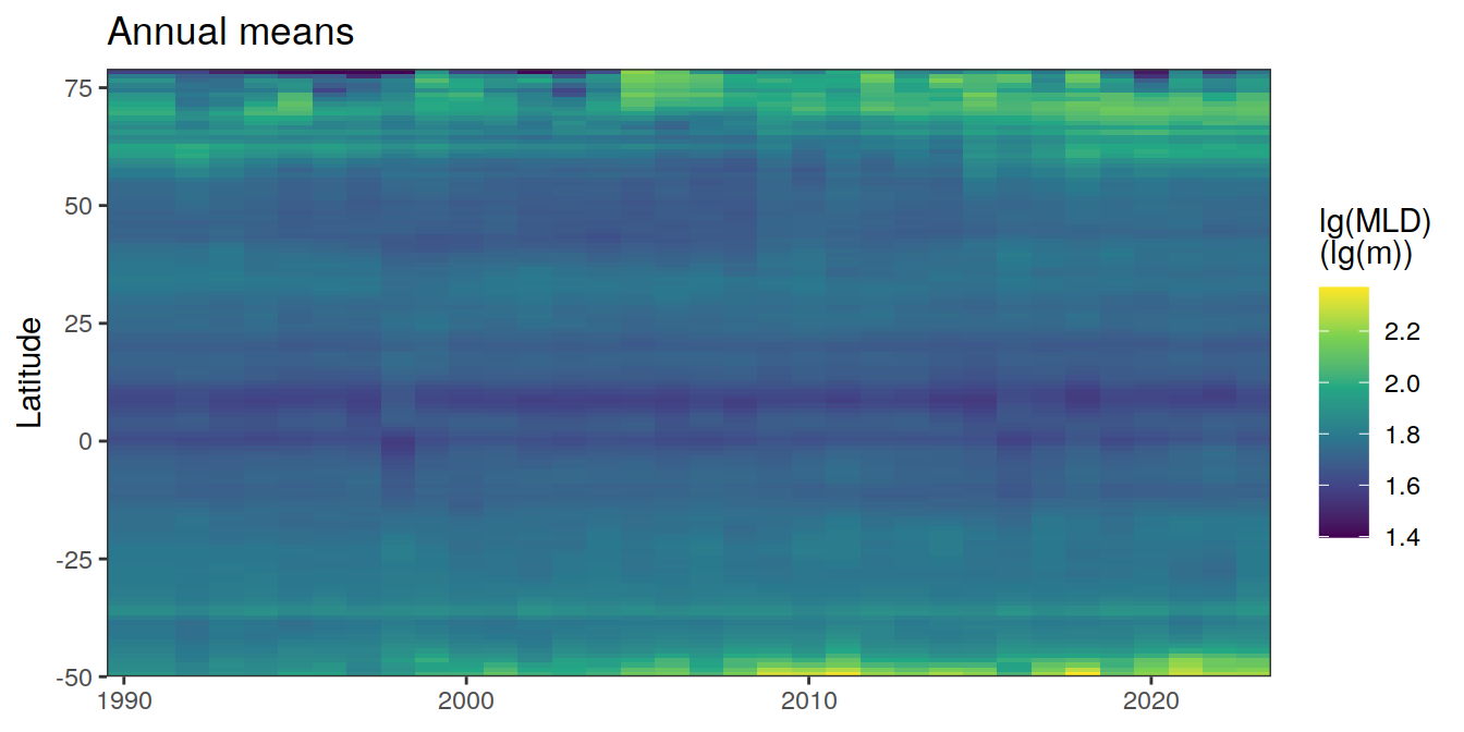
[[5]]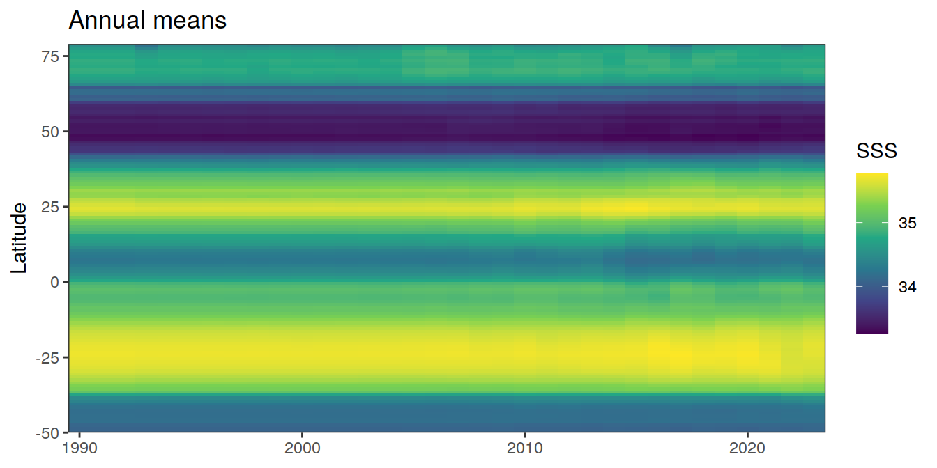
[[6]]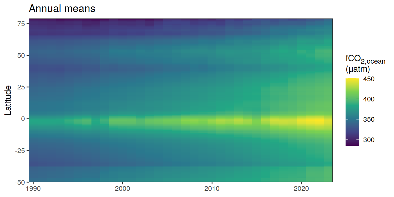
[[7]]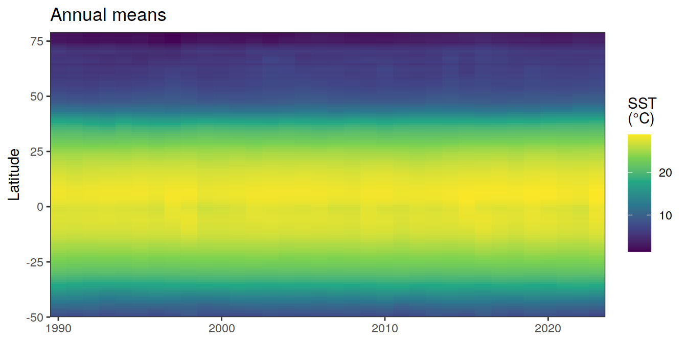
pco2_product_hovmoeller_monthly_annual %>%
  filter(name %in% name_divergent) %>%
  group_split(name) %>%
  # head(1) %>%
  map(
    ~ ggplot(data = .x,
             aes(year, lat, fill = value)) +
      geom_raster() +
      scale_fill_divergent(name = labels_breaks(.x %>% distinct(name))) +
      theme(legend.title = element_markdown()) +
      coord_cartesian(expand = 0) +
      labs(title = "Annual means",
           y = "Latitude") +
      theme(axis.title.x = element_blank())
  )
[[1]]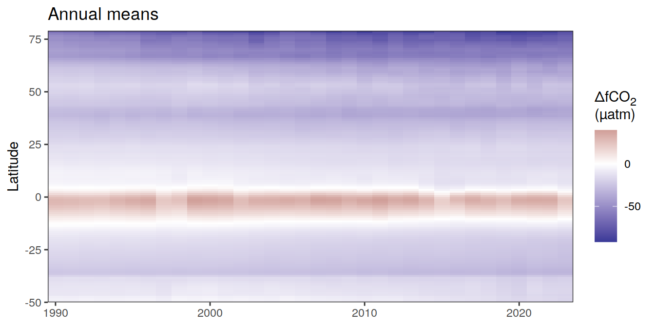
[[2]]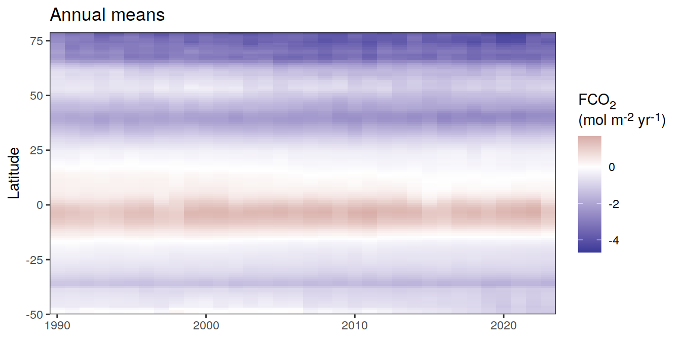
[[3]]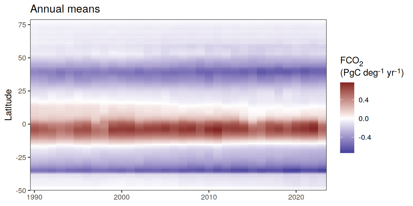
Monthly means
pco2_product_hovmoeller_monthly <-
  pco2_product %>%
  mutate(fgco2_int = fgco2) %>%
  select(-c(lon, time, biome)) %>%
  group_by(year, month, lat) %>%
  summarise(across(-c(fgco2_int, area),
                   ~ weighted.mean(., area, na.rm = TRUE)),
            across(fgco2_int,
                   ~ sum(. * area, na.rm = TRUE) * 12.01 * 1e-15)) %>%
  ungroup() %>%
  rename(fgco2_hov = fgco2_int) %>%
  filter(fgco2_hov != 0)


pco2_product_hovmoeller_monthly <-
  pco2_product_hovmoeller_monthly %>%
  pivot_longer(-c(year, month, lat)) %>%
  drop_na()

pco2_product_hovmoeller_monthly <-
  pco2_product_hovmoeller_monthly %>%
  mutate(decimal = year + (month-1) / 12)

pco2_product_hovmoeller_monthly %>%
  filter(!(name %in% name_divergent)) %>%
  group_split(name) %>%
  # head(1) %>%
  map(
    ~ ggplot(data = .x,
             aes(decimal, lat, fill = value)) +
      geom_raster() +
      scale_fill_viridis_c(name = labels_breaks(.x %>% distinct(name))) +
      theme(legend.title = element_markdown()) +
      labs(title = "Monthly means",
           y = "Latitude") +
      coord_cartesian(expand = 0) +
      theme(axis.title.x = element_blank())
  )
[[1]]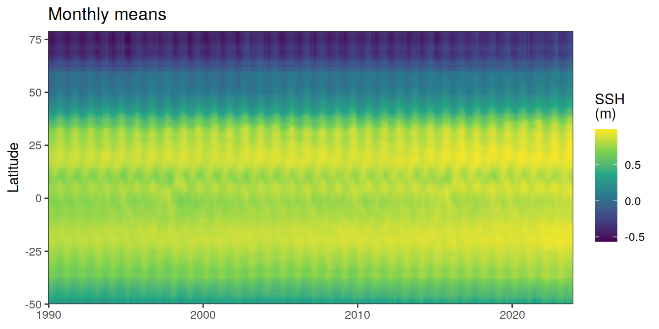
[[2]]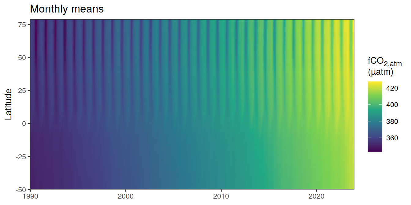
| Version | Author | Date |
|---|---|---|
| 009791f | jens-daniel-mueller | 2024-05-14 |
| 3b5d16b | jens-daniel-mueller | 2024-05-13 |
| e9c4ecf | jens-daniel-mueller | 2024-05-07 |
| 5d10d21 | jens-daniel-mueller | 2024-05-07 |
| dfcf790 | jens-daniel-mueller | 2024-04-11 |
| 89becff | jens-daniel-mueller | 2024-04-11 |
| 5c1676b | jens-daniel-mueller | 2024-03-24 |
| a1c2e14 | jens-daniel-mueller | 2024-03-24 |
[[3]]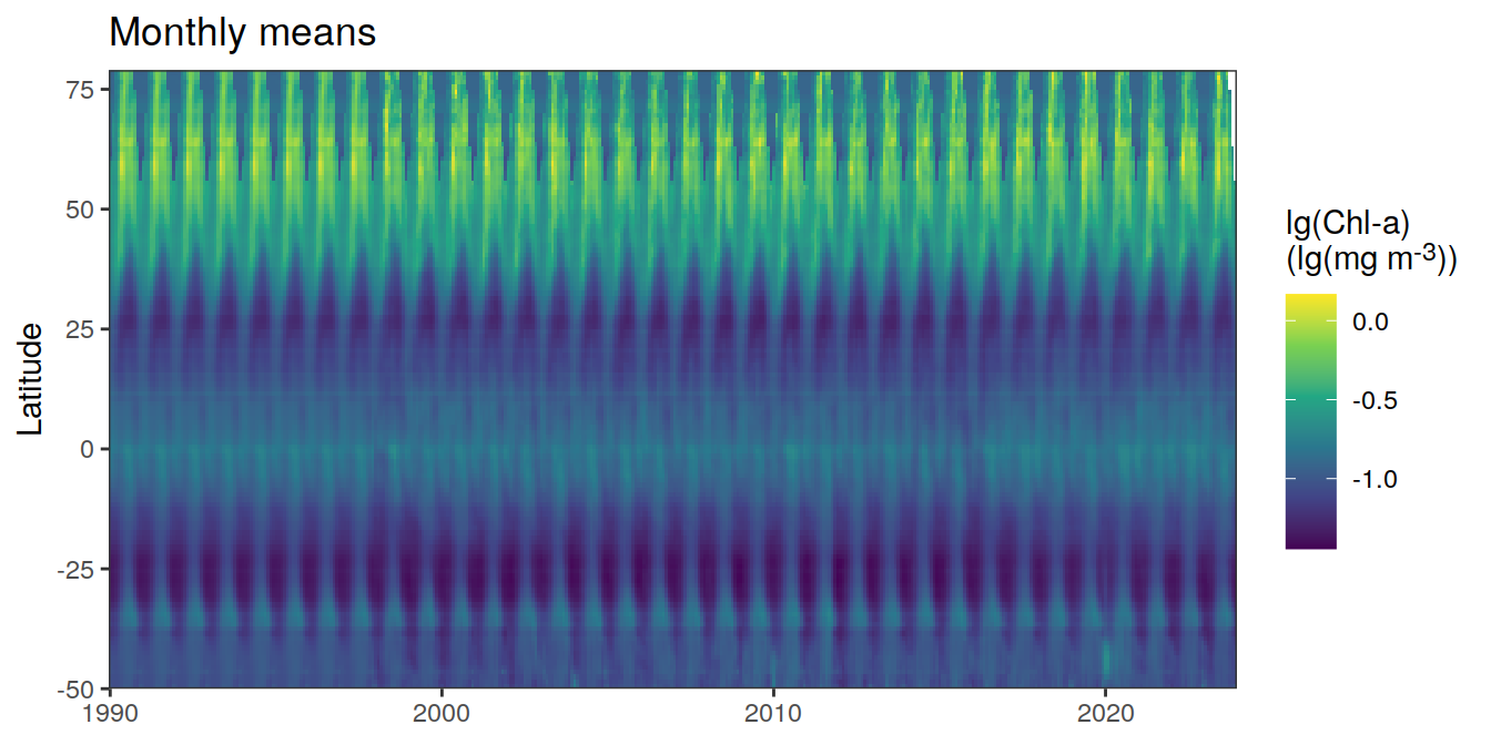
[[4]]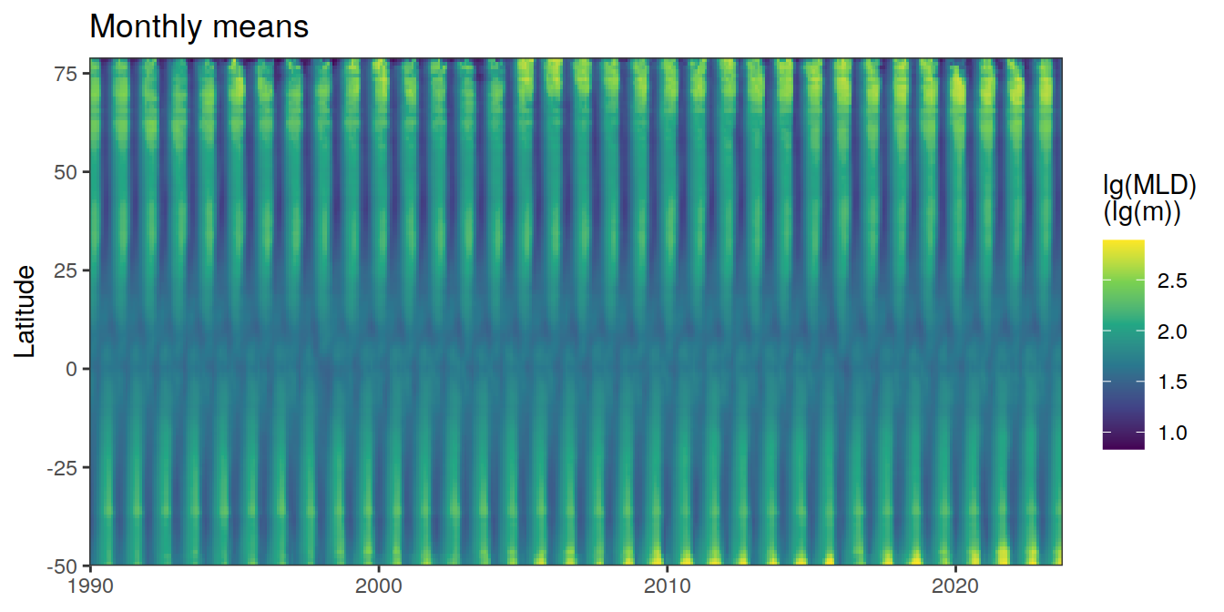
[[5]]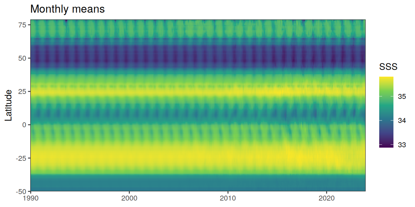
[[6]]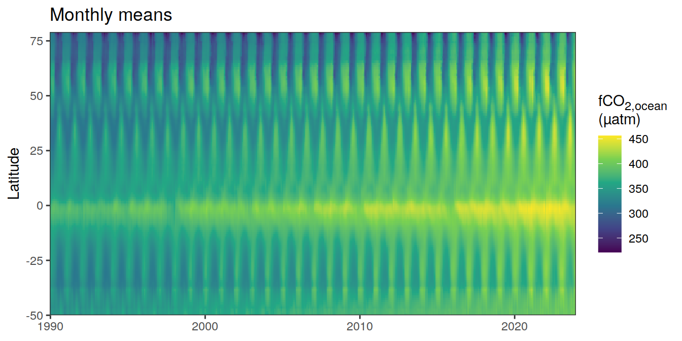
[[7]]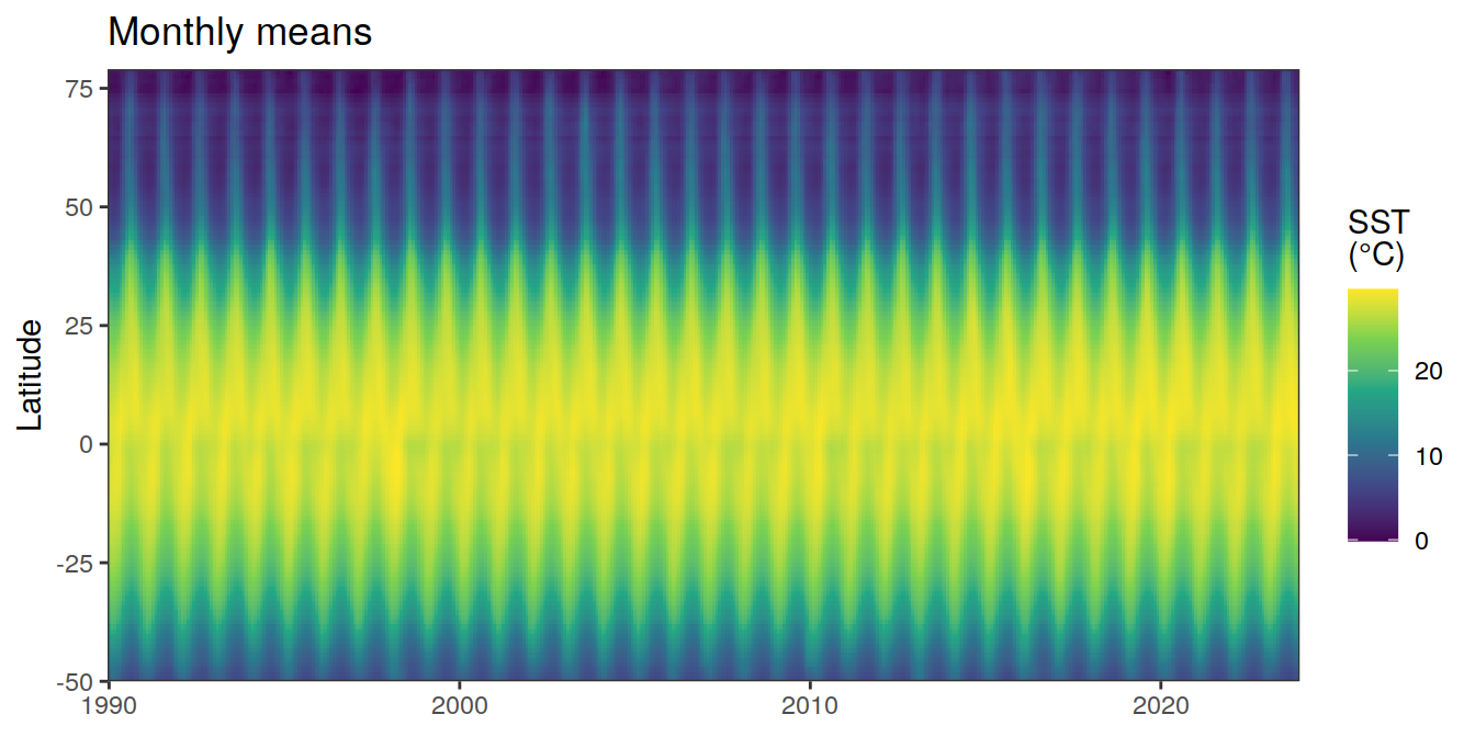
pco2_product_hovmoeller_monthly %>%
  filter(name %in% name_divergent) %>%
  group_split(name) %>%
  # head(1) %>%
  map(
    ~ ggplot(data = .x,
             aes(decimal, lat, fill = value)) +
      geom_raster() +
      scale_fill_divergent(name = labels_breaks(.x %>% distinct(name))) +
      theme(legend.title = element_markdown()) +
      labs(title = "Monthly means",
           y = "Latitude") +
      coord_cartesian(expand = 0) +
      theme(axis.title.x = element_blank())
  )
[[1]]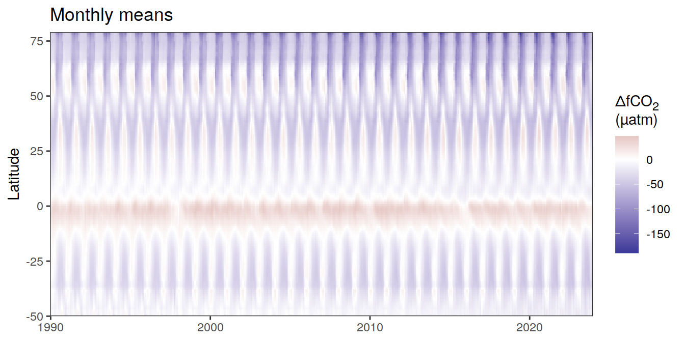
[[2]]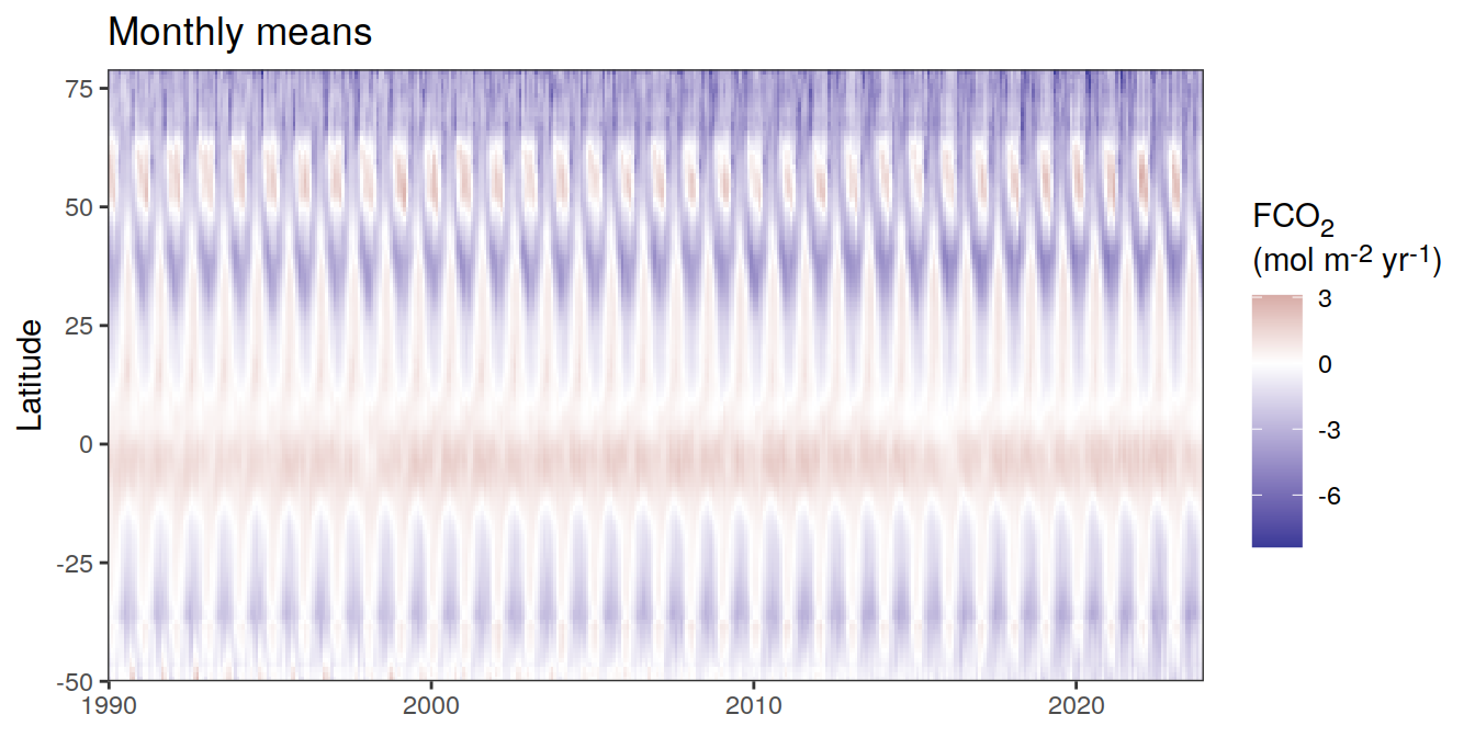
[[3]]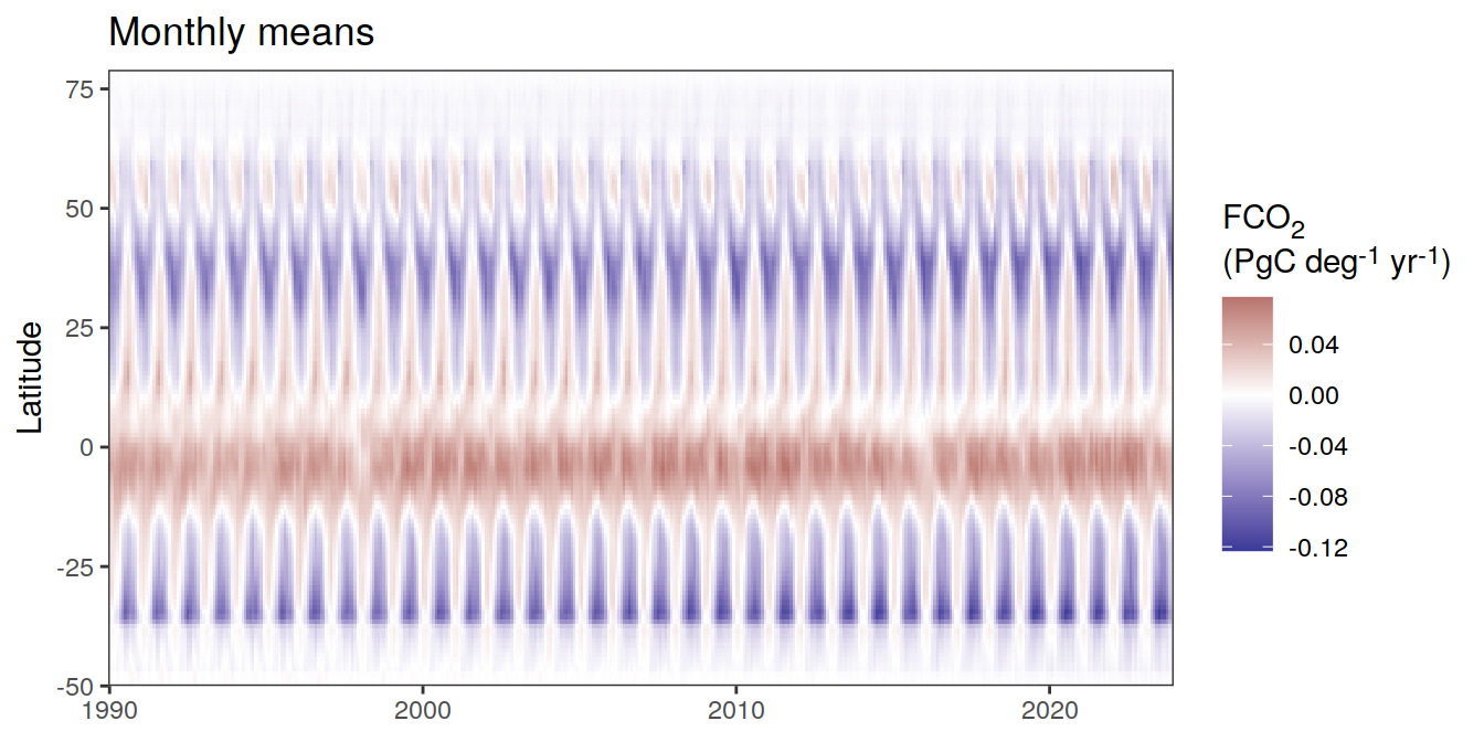
pCO2productanalysis_2023 <-
  knitr::knit_expand(
    file = here::here("analysis/child/pCO2_product_analysis.Rmd"),
    product_name = "CMEMS",
    year_anom = 2023
  )
2023 anomalies
Detection
For the detection of anomalies at any point in time and space, we fit regression models and compare the fitted to the actual value.
We use linear regression models for all parameters, except for , which are approximated with quadratic fits.
The regression models are fitted to all data since , except 2023.
anomaly_determination <- function(df,...) {

  group_by <- quos(...)
  # group_by <- quos(lon, lat)
  # df <- pco2_product_coarse_annual

  # Linear regression models

  df_lm <-
    df %>%
    filter(year != 2023,
           !(name %in% name_quadratic_fit)) %>%
    nest(data = -c(name, !!!group_by)) %>%
    mutate(
      fit = map(data, ~ lm(value ~ year, data = .x)),
      tidied = map(fit, tidy),
      augmented = map(fit, augment)
    )


  df_lm_year_anom <-
    full_join(
      df_lm %>%
        unnest(tidied) %>%
        select(name, !!!group_by, term, estimate) %>%
        pivot_wider(names_from = term,
                    values_from = estimate) %>%
        mutate(fit = `(Intercept)` + year * 2023) %>%
        select(name, !!!group_by, fit) %>%
        mutate(year = 2023),
      df %>%
        filter(year == 2023,
               !(name %in% name_quadratic_fit))
    ) %>%
    mutate(resid = value - fit)


  df_lm <-
    bind_rows(
      df_lm %>%
        unnest(augmented) %>%
        select(name, !!!group_by, year, value, fit = .fitted, resid = .resid),
      df_lm_year_anom
    )

  rm(df_lm_year_anom)

  # Quadratic regression models

  df_quadratic <-
    df %>%
    filter(year != 2023,
           name %in% name_quadratic_fit) %>%
    nest(data = -c(name, !!!group_by)) %>%
    mutate(
      fit = map(data, ~ lm(value ~ year + I(year ^ 2), data = .x)),
      tidied = map(fit, tidy),
      augmented = map(fit, augment)
    )


  df_quadratic_year_anom <-
    full_join(
      df_quadratic %>%
        unnest(tidied) %>%
        select(name, !!!group_by, term, estimate) %>%
        pivot_wider(names_from = term,
                    values_from = estimate) %>%
        mutate(fit = `(Intercept)` + year * 2023 + `I(year^2)` * 2023 ^ 2) %>%
        select(name, !!!group_by, fit) %>%
        mutate(year = 2023),
      df %>%
        filter(year == 2023,
               name %in% name_quadratic_fit)
    ) %>%
    mutate(resid = value - fit)


  df_quadratic <-
    bind_rows(
      df_quadratic %>%
        unnest(augmented) %>%
        select(name, !!!group_by, year, value, fit = .fitted, resid = .resid),
      df_quadratic_year_anom
    )

  rm(df_quadratic_year_anom)

  # Join linear and quadratic regression results

  df_regression <-
    bind_rows(df_lm,
              df_quadratic)

  df_regression <-
    df_regression %>%
    arrange(year)

  rm(df_lm,
     df_quadratic)


  return(df_regression)

}
anomaly_determination <- function(df,...) {
group_by <- quos(...)
# group_by <- quos(biome)
# group_by <- quos(lon, lat)
# df <- pco2_product_coarse_annual
# Climatoligcal mean
df_mean <-
df %>%
filter(year < 2023,
year >= 2023-5) %>%
group_by(name, !!!group_by) %>%
summarize(
fit = mean(value, na.rm = TRUE)
) %>%
ungroup()
df_mean <-
full_join(
df_mean,
df
) %>%
mutate(resid = value - fit)
return(df_mean)
}Maps
The following maps show the absolute state of each variable in 2023 as provided through the pCO2 product, the change in that variable from 1990 to 2023, as well es the anomalies in 2023. Changes and anomalies are determined based on the predicted value of a linear regression model fit to the data from 1990 to 2022.
Maps are first presented as annual means, and than as monthly means. Note that the 2023 predictions for the monthly maps are done individually for each month, such the mean seasonal anomaly from the annual mean is removed.
Note: The increase the computational speed, I regridded all maps to 5X5° grid.
Annual means
2023 absolute
pco2_product_coarse_annual_regression <-
  pco2_product_coarse_annual %>%
  drop_na() %>%
  anomaly_determination(lon, lat)

pco2_product_coarse_annual_regression <-
  pco2_product_coarse_annual_regression %>%
  drop_na()

pco2_product_coarse_annual_regression %>%
  filter(year == 2023,
         !(name %in% name_divergent)) %>%
  group_split(name) %>%
  # head(1) %>%
  map(
    ~ map +
      geom_tile(data = .x,
                aes(lon, lat, fill = value)) +
      labs(title = paste("Annual mean", 2023)) +
      scale_fill_viridis_c(name = labels_breaks(.x %>% distinct(name))) +
      theme(legend.title = element_markdown())
  )
[[1]]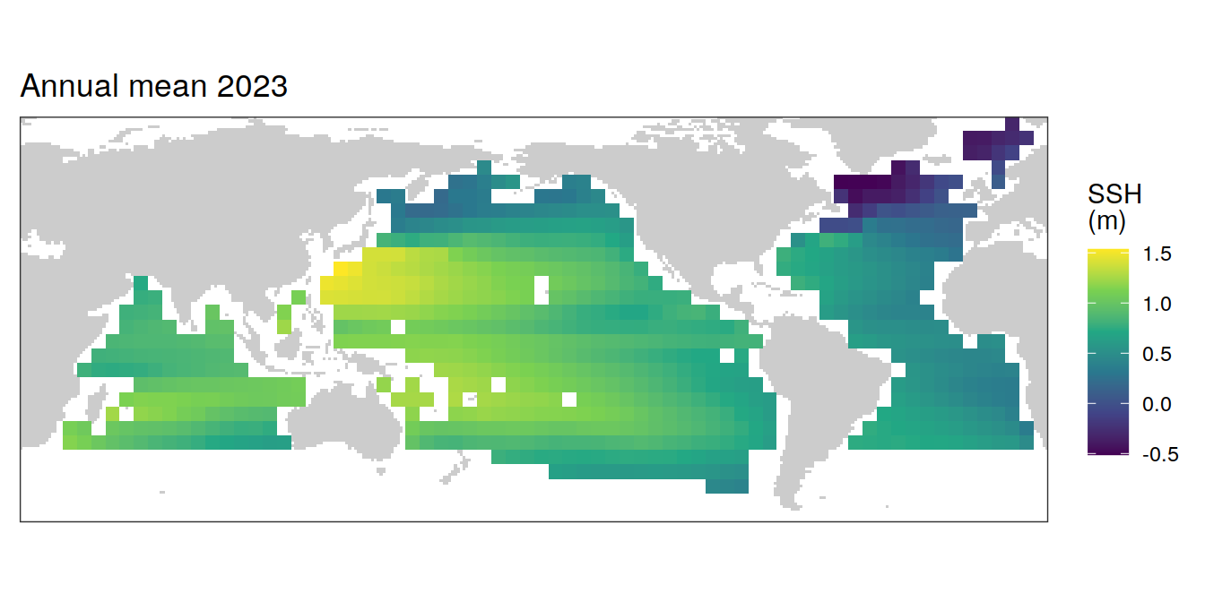
| Version | Author | Date |
|---|---|---|
| 009791f | jens-daniel-mueller | 2024-05-14 |
| 77accd5 | jens-daniel-mueller | 2024-05-07 |
| 5d10d21 | jens-daniel-mueller | 2024-05-07 |
| dfcf790 | jens-daniel-mueller | 2024-04-11 |
| 89becff | jens-daniel-mueller | 2024-04-11 |
| 2321242 | jens-daniel-mueller | 2024-04-11 |
| c9d994c | jens-daniel-mueller | 2024-04-04 |
| a1c2e14 | jens-daniel-mueller | 2024-03-24 |
[[2]]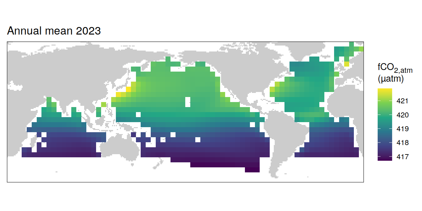
| Version | Author | Date |
|---|---|---|
| 009791f | jens-daniel-mueller | 2024-05-14 |
| 3b5d16b | jens-daniel-mueller | 2024-05-13 |
| 77accd5 | jens-daniel-mueller | 2024-05-07 |
| e9c4ecf | jens-daniel-mueller | 2024-05-07 |
| 5d10d21 | jens-daniel-mueller | 2024-05-07 |
| dfcf790 | jens-daniel-mueller | 2024-04-11 |
| 89becff | jens-daniel-mueller | 2024-04-11 |
| 2321242 | jens-daniel-mueller | 2024-04-11 |
| c9d994c | jens-daniel-mueller | 2024-04-04 |
| 5c1676b | jens-daniel-mueller | 2024-03-24 |
| a1c2e14 | jens-daniel-mueller | 2024-03-24 |
[[3]]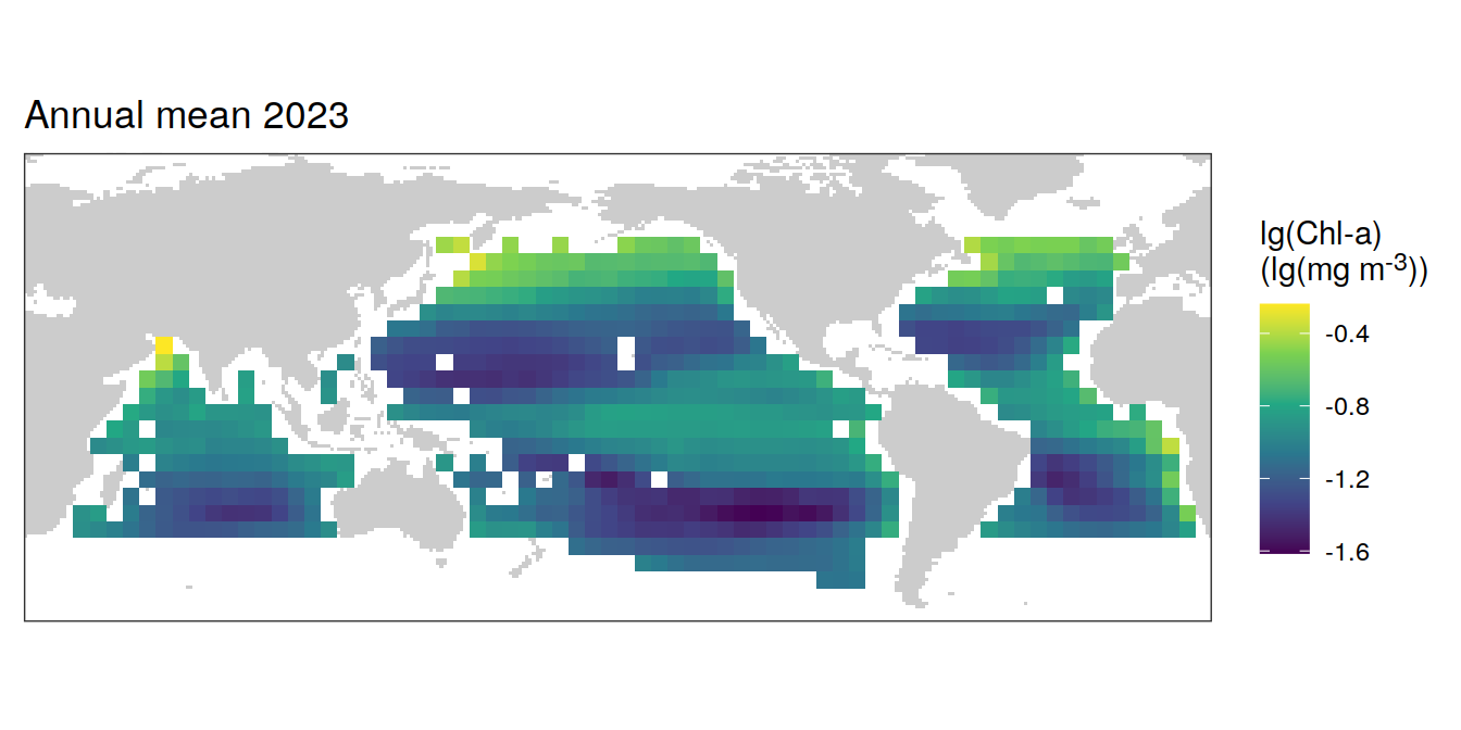
[[4]]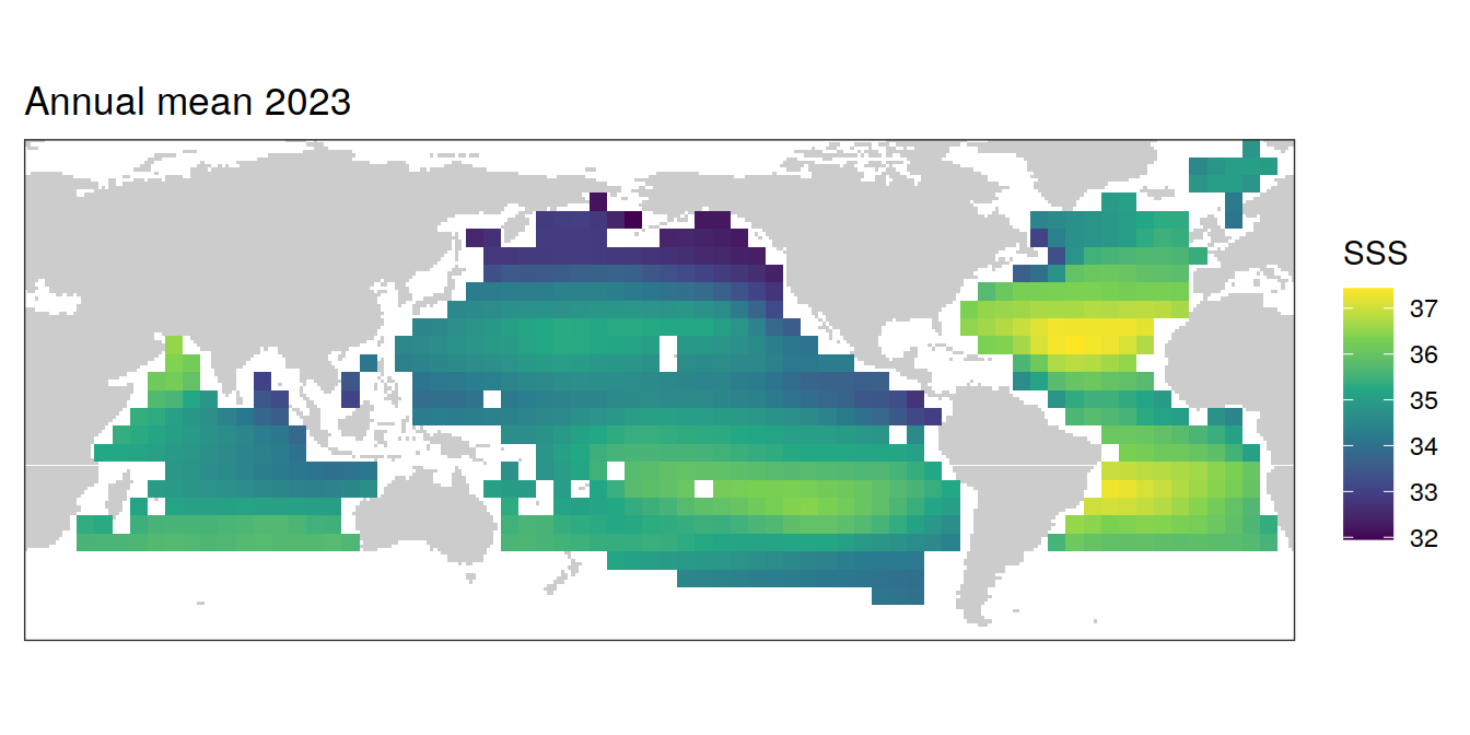
[[5]]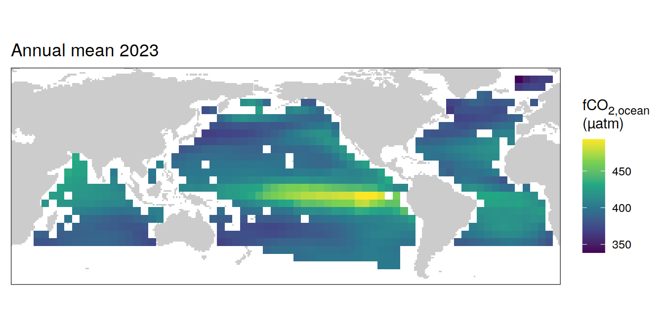
[[6]]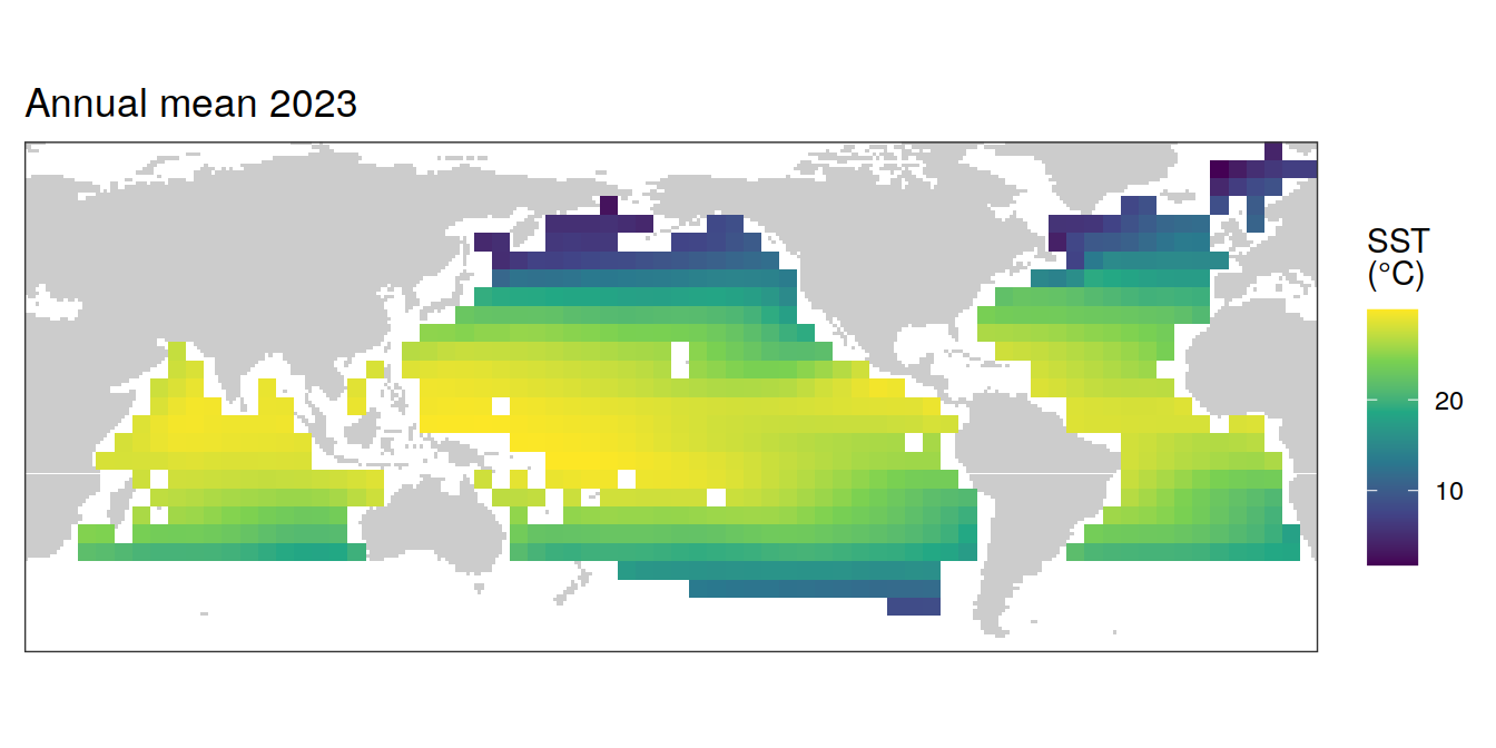
pco2_product_coarse_annual_regression %>%
  filter(year == 2023,
         name %in% name_divergent) %>%
  group_split(name) %>%
  # head(1) %>%
  map( ~ map +
         geom_tile(data = .x,
                   aes(lon, lat, fill = value)) +
         labs(title = paste("Annual mean", 2023)) +
         scale_fill_divergent(
           name = labels_breaks(.x %>% distinct(name))) +
         theme(legend.title = element_markdown())
  )
[[1]]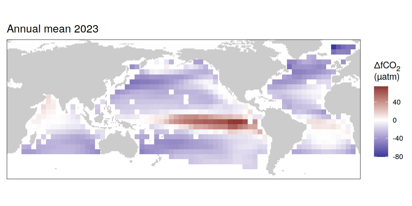
[[2]]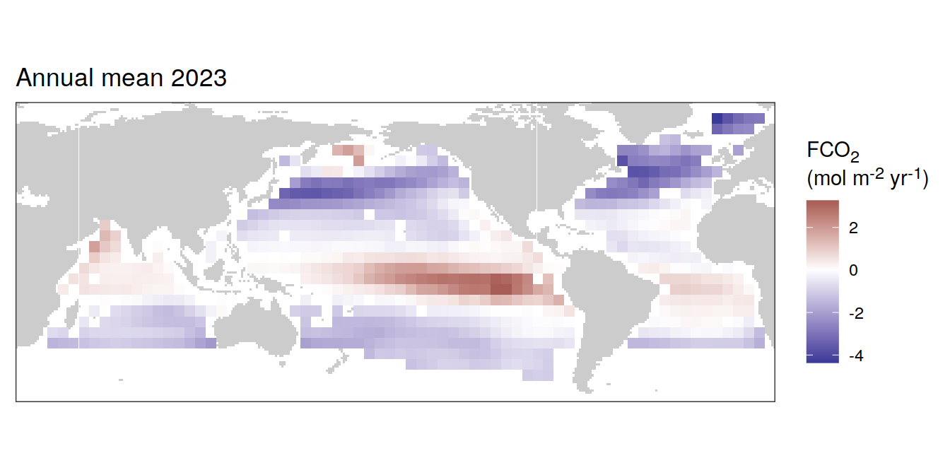
Trends
pco2_product_coarse_annual_regression <-
  pco2_product_coarse_annual_regression %>%
  group_by(name) %>%
  filter(year %in% c(min(year), max(year), 2023)) %>%
  ungroup()

pco2_product_coarse_annual_regression %>%
  select(-c(value, resid)) %>%
  filter(year %in% c(min(year), max(year))) %>%
  arrange(year) %>%
  group_by(lon, lat, name) %>%
  mutate(change = fit - lag(fit),
         period = paste(lag(year), year, sep = "-")) %>%
  ungroup() %>%
  filter(!is.na(change)) %>%
  group_split(name) %>%
  # head(1) %>%
  map(
    ~ map +
      geom_tile(data = .x,
                aes(lon, lat, fill = change)) +
      labs(title =  paste("Change: ",.x$period)) +
      scale_fill_divergent(name = labels_breaks(.x %>% distinct(name))) +
      theme(legend.title = element_markdown())
  )
[[1]]
[[2]]
[[3]]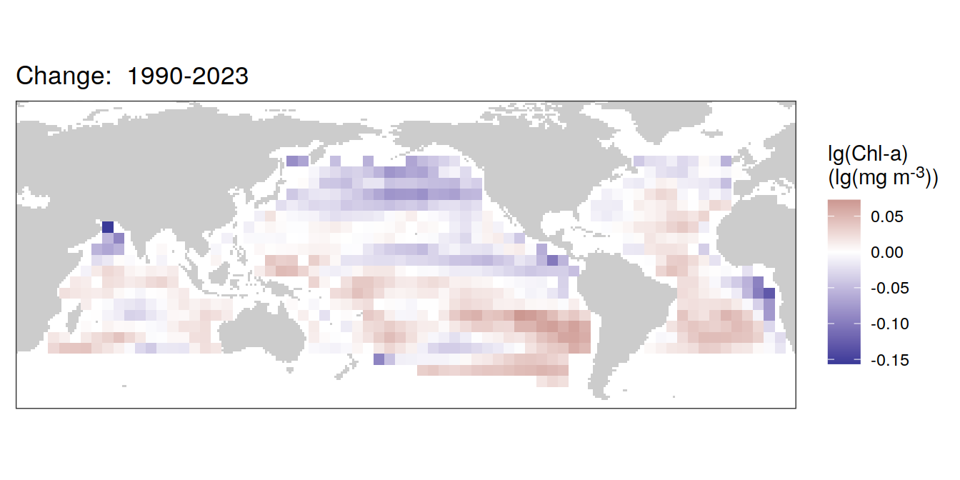
[[4]]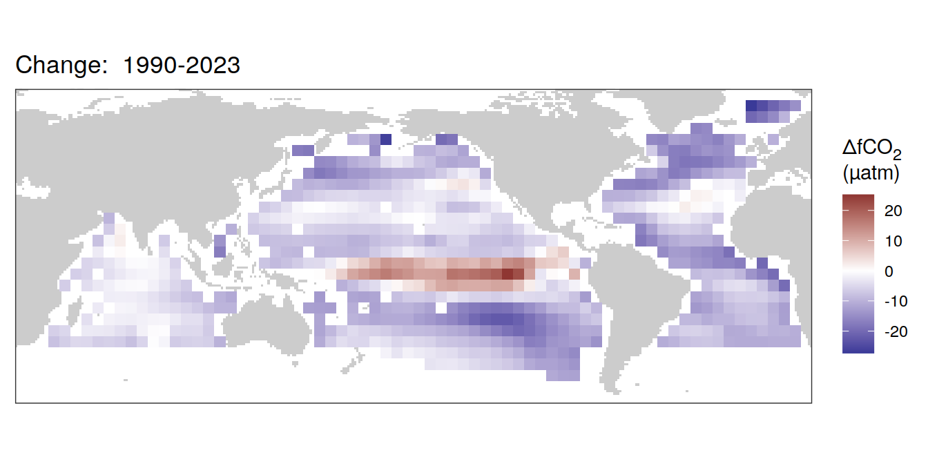
[[5]]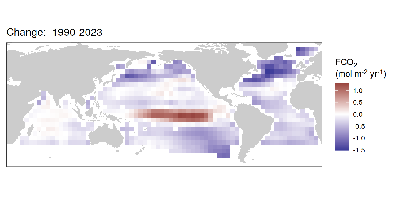
[[6]]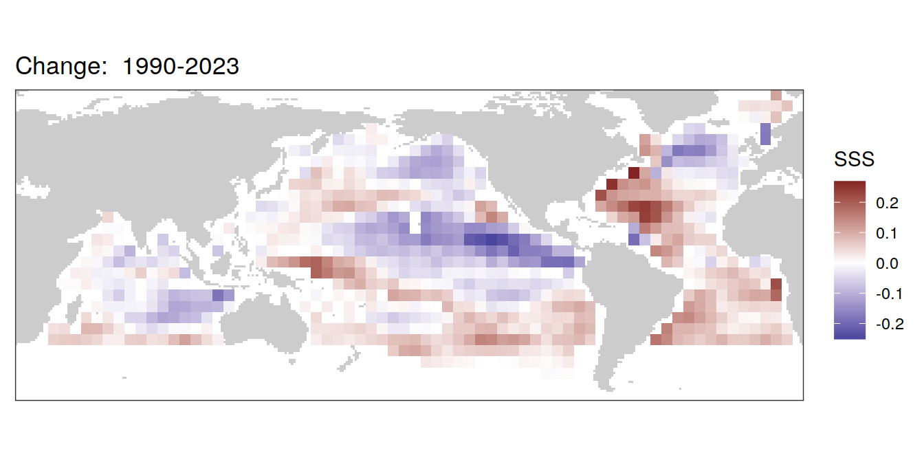
[[7]]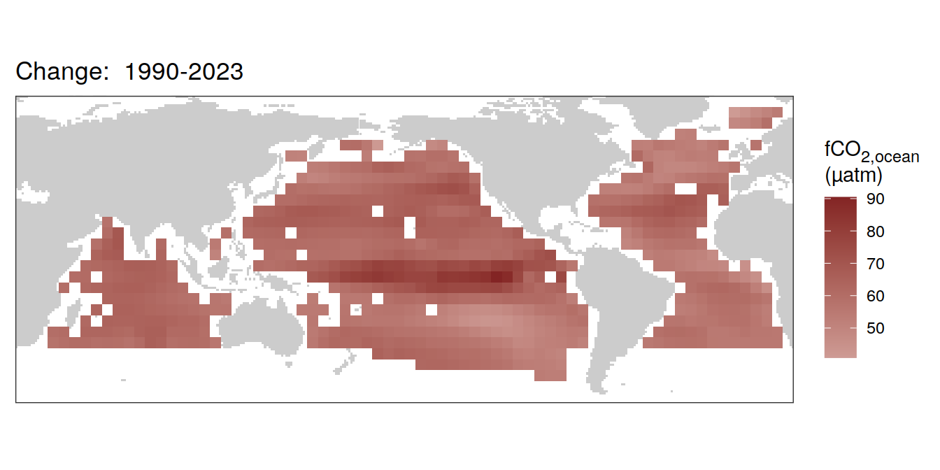
[[8]]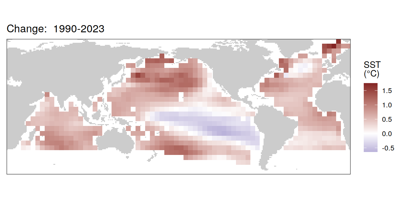
2023 anomaly
pco2_product_coarse_annual_regression %>%
  filter(year == 2023) %>%
  group_split(name) %>%
  # head(1) %>%
  map( ~ map +
         geom_tile(data = .x,
                   aes(lon, lat, fill = resid)) +
         labs(title =  paste(2023,"anomaly")) +
         scale_fill_divergent(
           name = labels_breaks(.x %>% distinct(name))) +
         theme(legend.title = element_markdown())
  )
[[1]]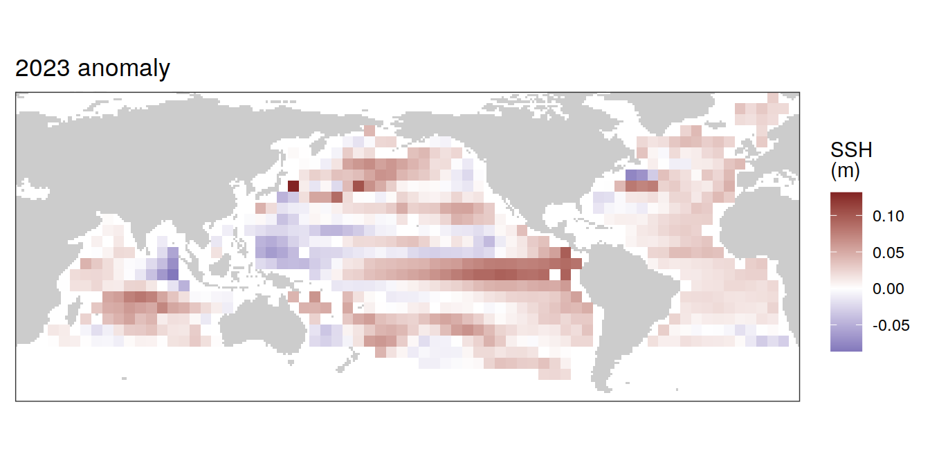
[[2]]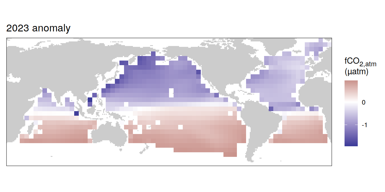
| Version | Author | Date |
|---|---|---|
| 009791f | jens-daniel-mueller | 2024-05-14 |
| 3b5d16b | jens-daniel-mueller | 2024-05-13 |
| 77accd5 | jens-daniel-mueller | 2024-05-07 |
| e9c4ecf | jens-daniel-mueller | 2024-05-07 |
| 5d10d21 | jens-daniel-mueller | 2024-05-07 |
| dfcf790 | jens-daniel-mueller | 2024-04-11 |
| 89becff | jens-daniel-mueller | 2024-04-11 |
| 2321242 | jens-daniel-mueller | 2024-04-11 |
[[3]]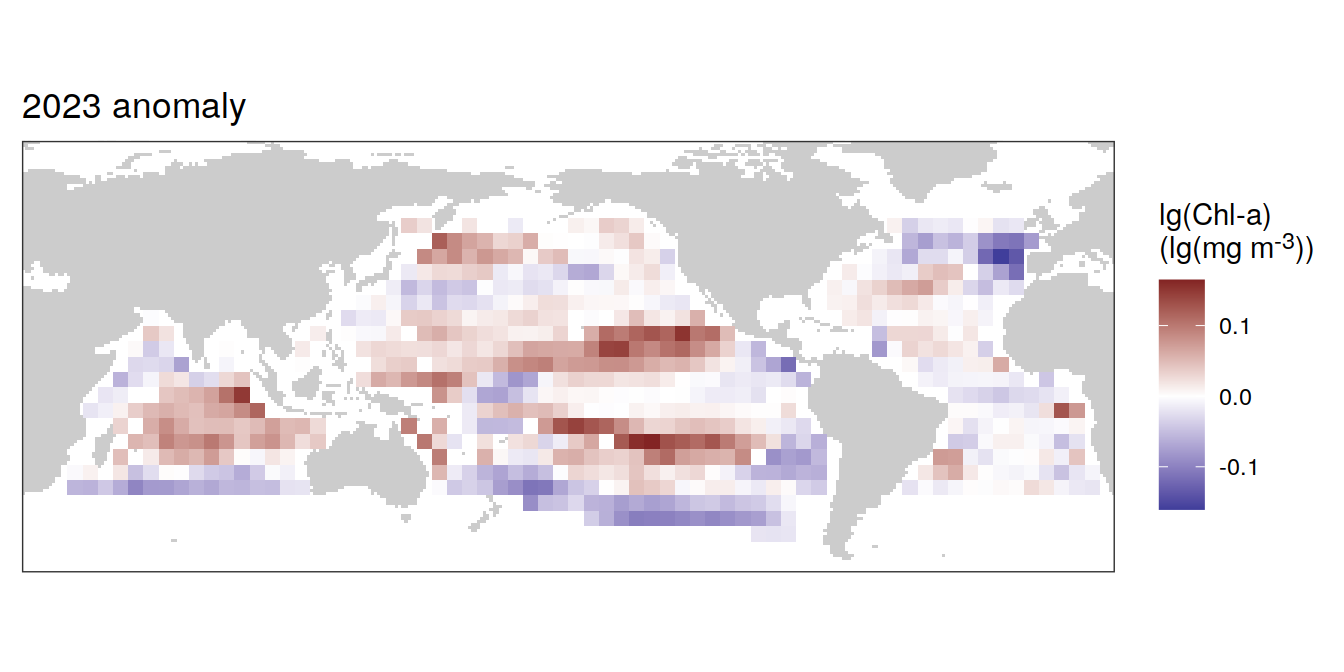
[[4]]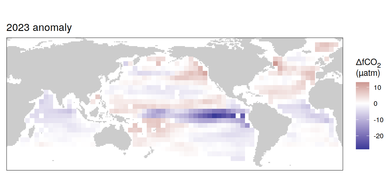
[[5]]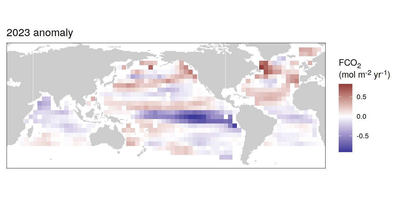
[[6]]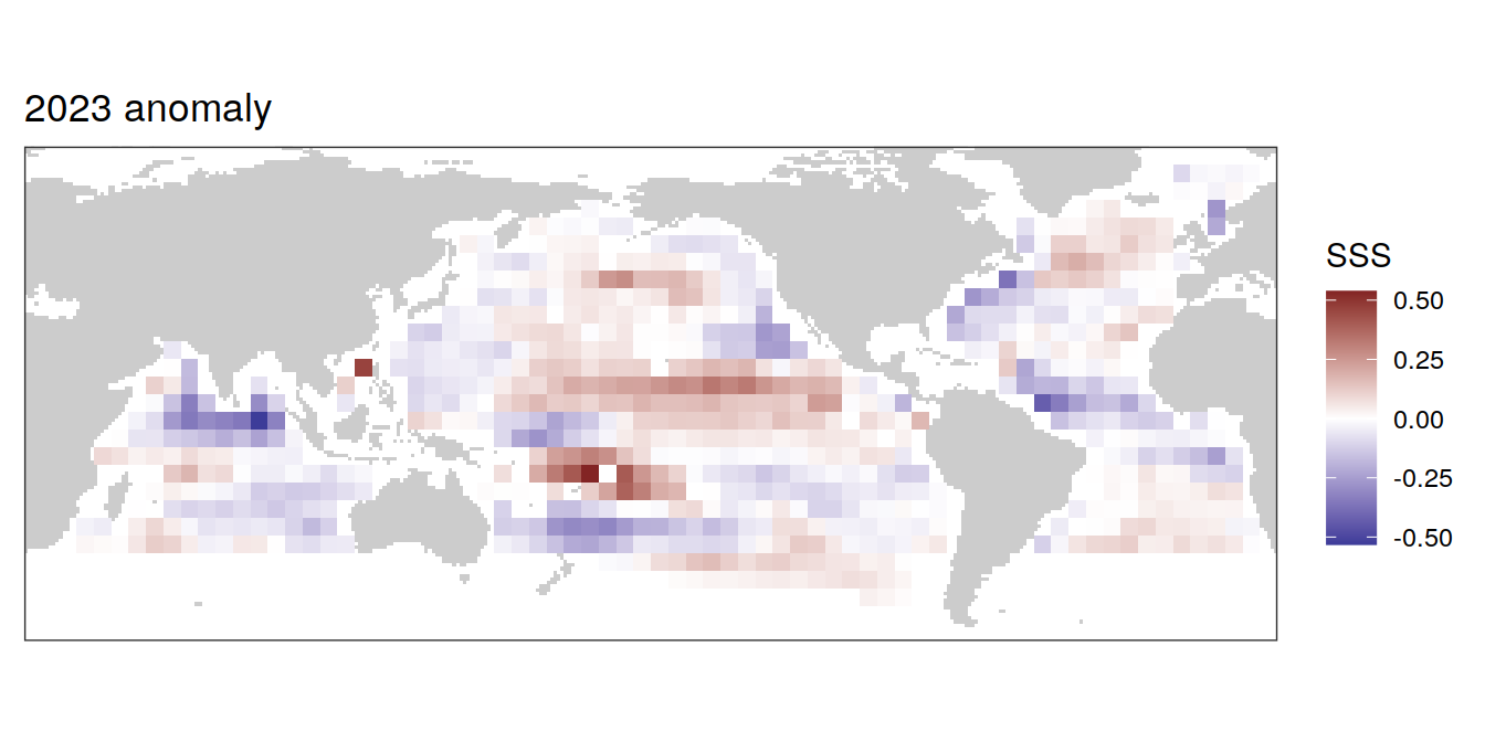
[[7]]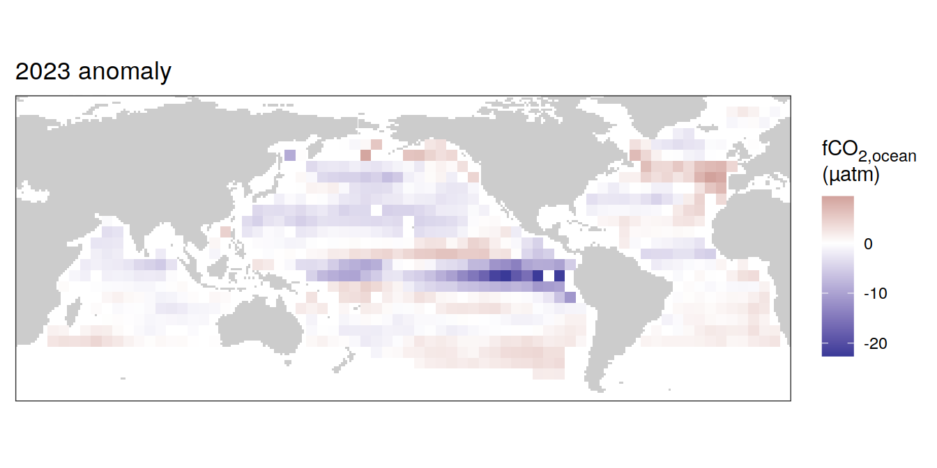
[[8]]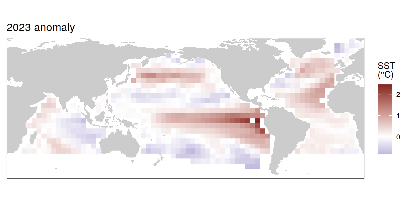
pco2_product_coarse_annual_regression %>%
  write_csv(paste0("../data/","CMEMS","_","2023","_anomaly_map_annual.csv"))
Monthly means
2023 absolute
pco2_product_coarse_monthly_regression <-
  pco2_product_coarse_monthly %>%
  drop_na() %>%
  anomaly_determination(lon, lat, month)

pco2_product_coarse_monthly_regression <-
  pco2_product_coarse_monthly_regression %>%
  drop_na()


pco2_product_coarse_monthly_regression %>%
  filter(year == 2023,
         !(name %in% name_divergent)) %>%
  group_split(name) %>%
  # head(1) %>%
  map(
    ~ map +
      geom_tile(data = .x,
                aes(lon, lat, fill = value)) +
      labs(title = paste("Monthly means", 2023)) +
      scale_fill_viridis_c(name = labels_breaks(.x %>% distinct(name))) +
      theme(legend.title = element_markdown()) +
      facet_wrap( ~ month, ncol = 2)
  )
[[1]]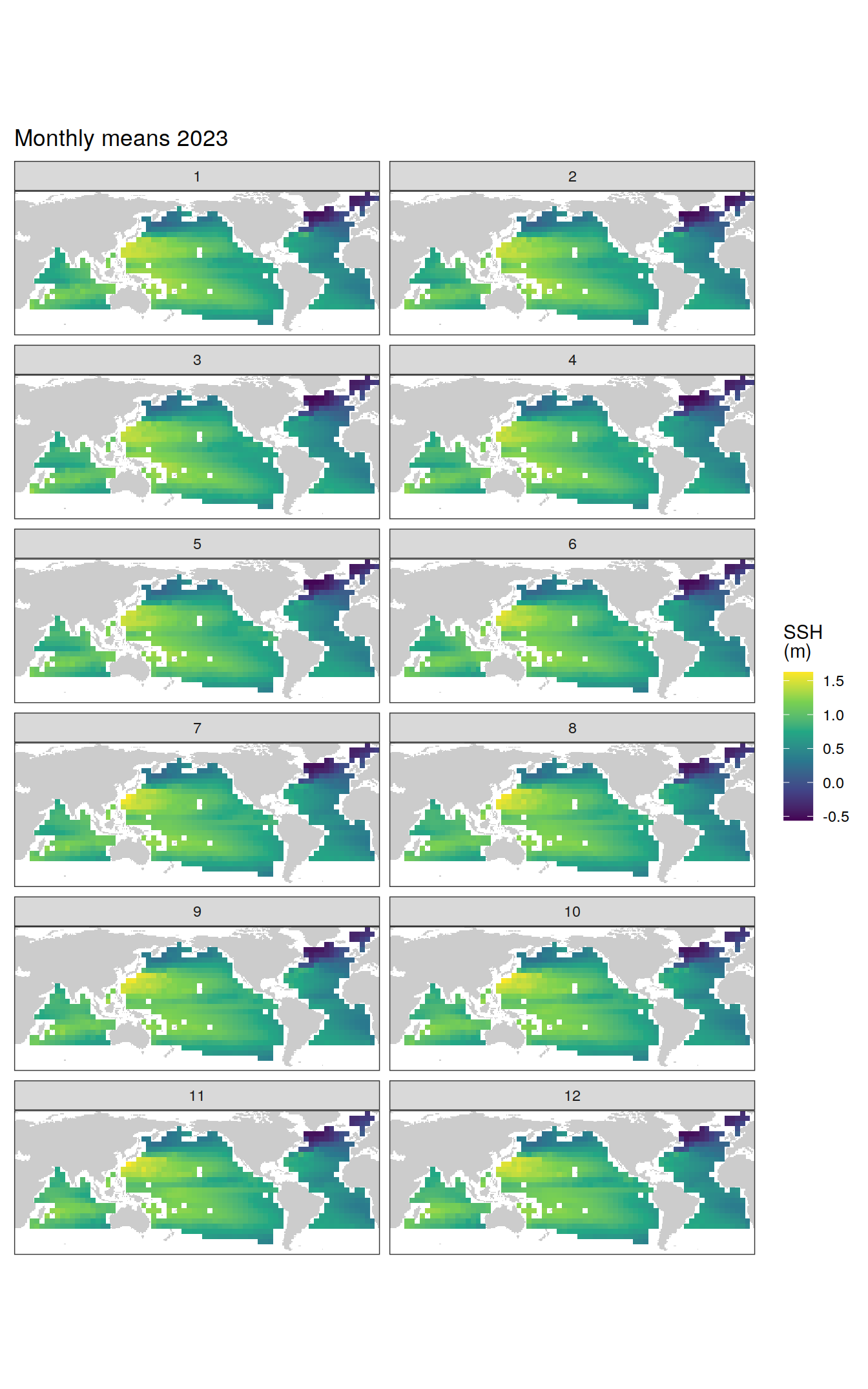
| Version | Author | Date |
|---|---|---|
| 009791f | jens-daniel-mueller | 2024-05-14 |
| 77accd5 | jens-daniel-mueller | 2024-05-07 |
| 5d10d21 | jens-daniel-mueller | 2024-05-07 |
| dfcf790 | jens-daniel-mueller | 2024-04-11 |
| 89becff | jens-daniel-mueller | 2024-04-11 |
| 2321242 | jens-daniel-mueller | 2024-04-11 |
| c9d994c | jens-daniel-mueller | 2024-04-04 |
| a1c2e14 | jens-daniel-mueller | 2024-03-24 |
[[2]]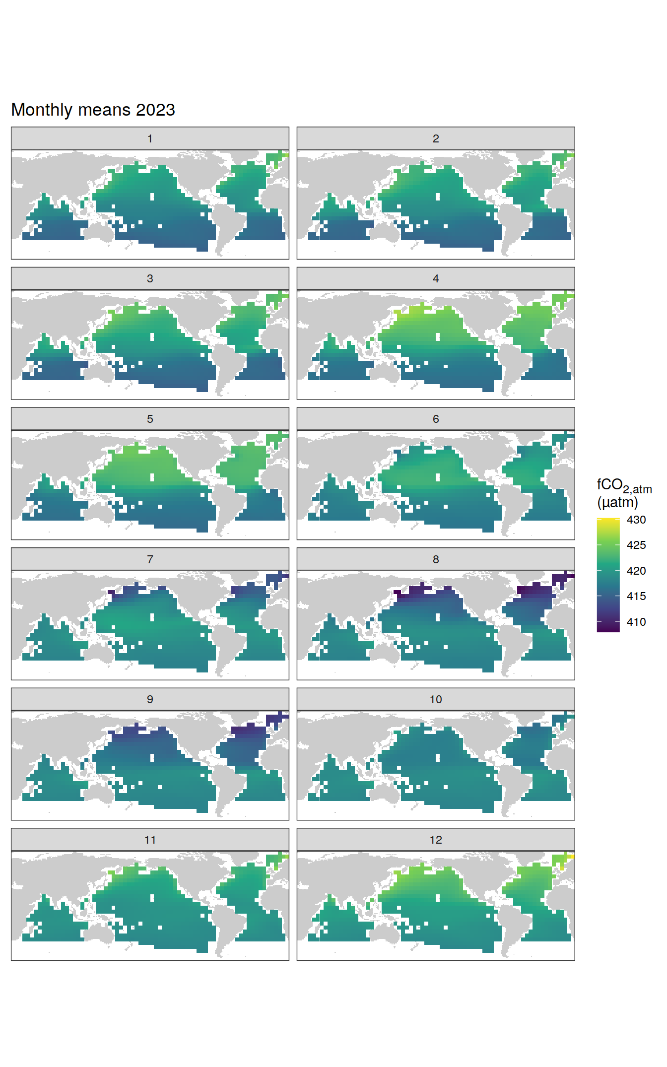
| Version | Author | Date |
|---|---|---|
| 009791f | jens-daniel-mueller | 2024-05-14 |
| 3b5d16b | jens-daniel-mueller | 2024-05-13 |
| 77accd5 | jens-daniel-mueller | 2024-05-07 |
| e9c4ecf | jens-daniel-mueller | 2024-05-07 |
| 5d10d21 | jens-daniel-mueller | 2024-05-07 |
| dfcf790 | jens-daniel-mueller | 2024-04-11 |
| 89becff | jens-daniel-mueller | 2024-04-11 |
| 2321242 | jens-daniel-mueller | 2024-04-11 |
| c9d994c | jens-daniel-mueller | 2024-04-04 |
| 5c1676b | jens-daniel-mueller | 2024-03-24 |
| a1c2e14 | jens-daniel-mueller | 2024-03-24 |
[[3]]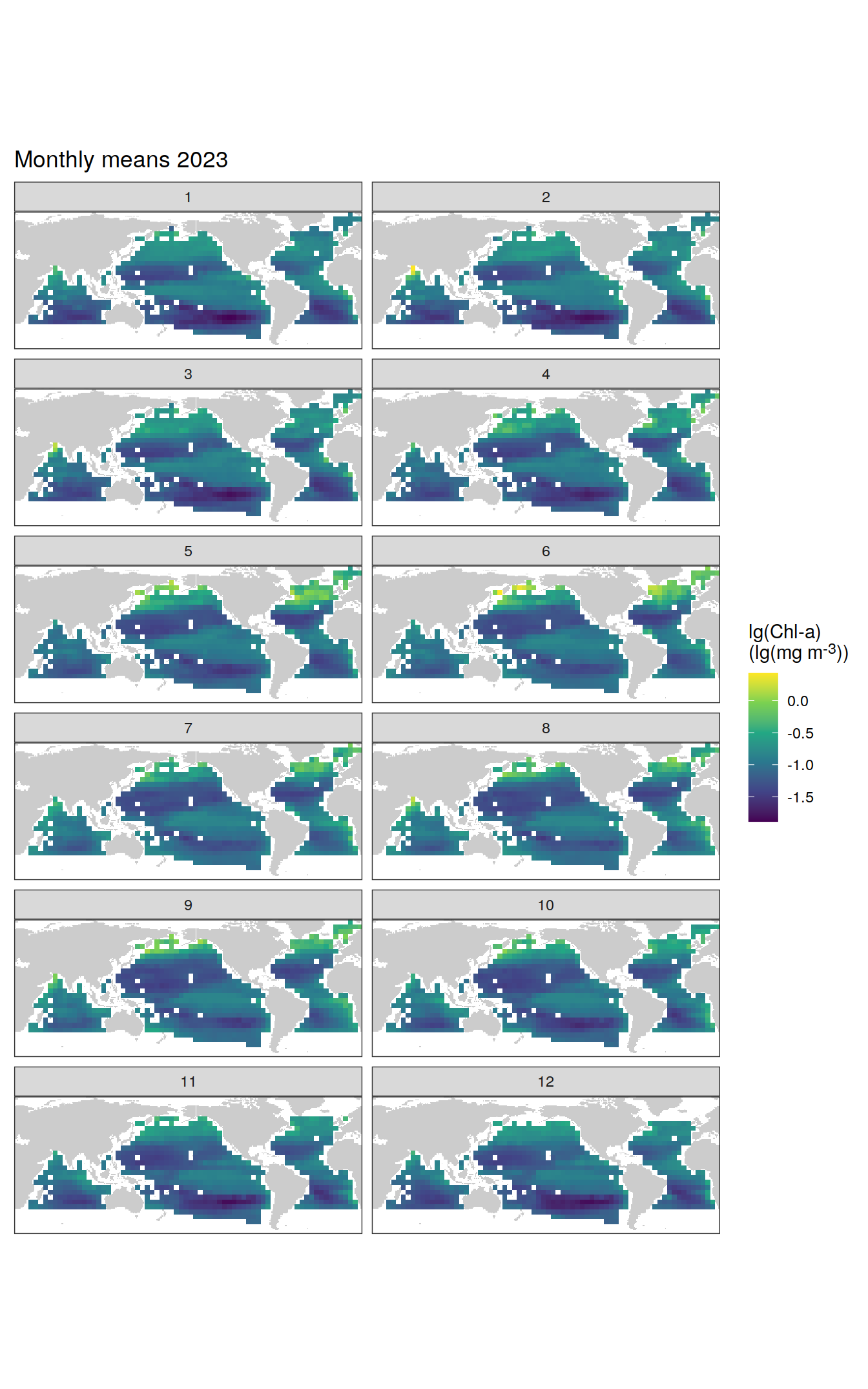
[[4]]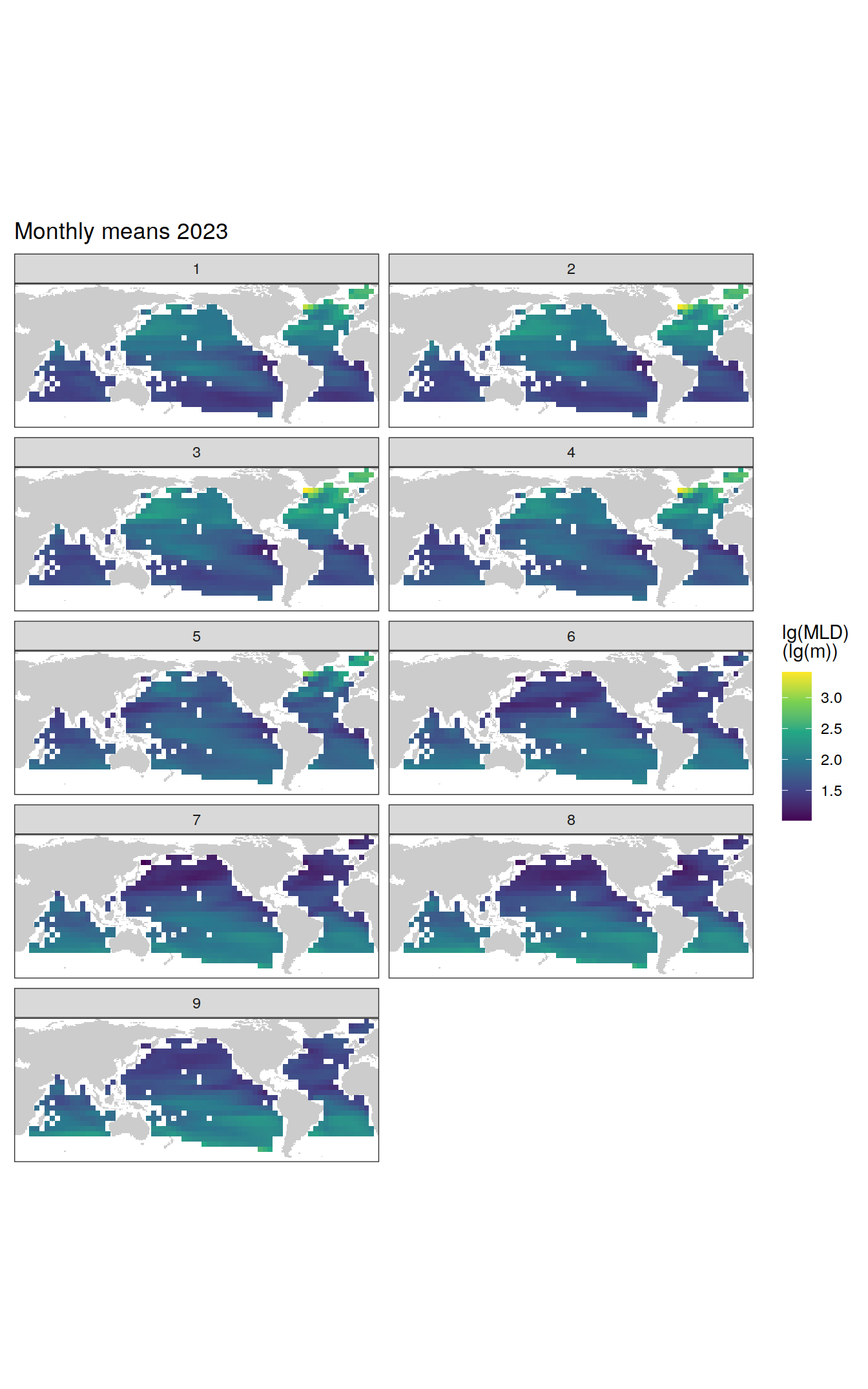
[[5]]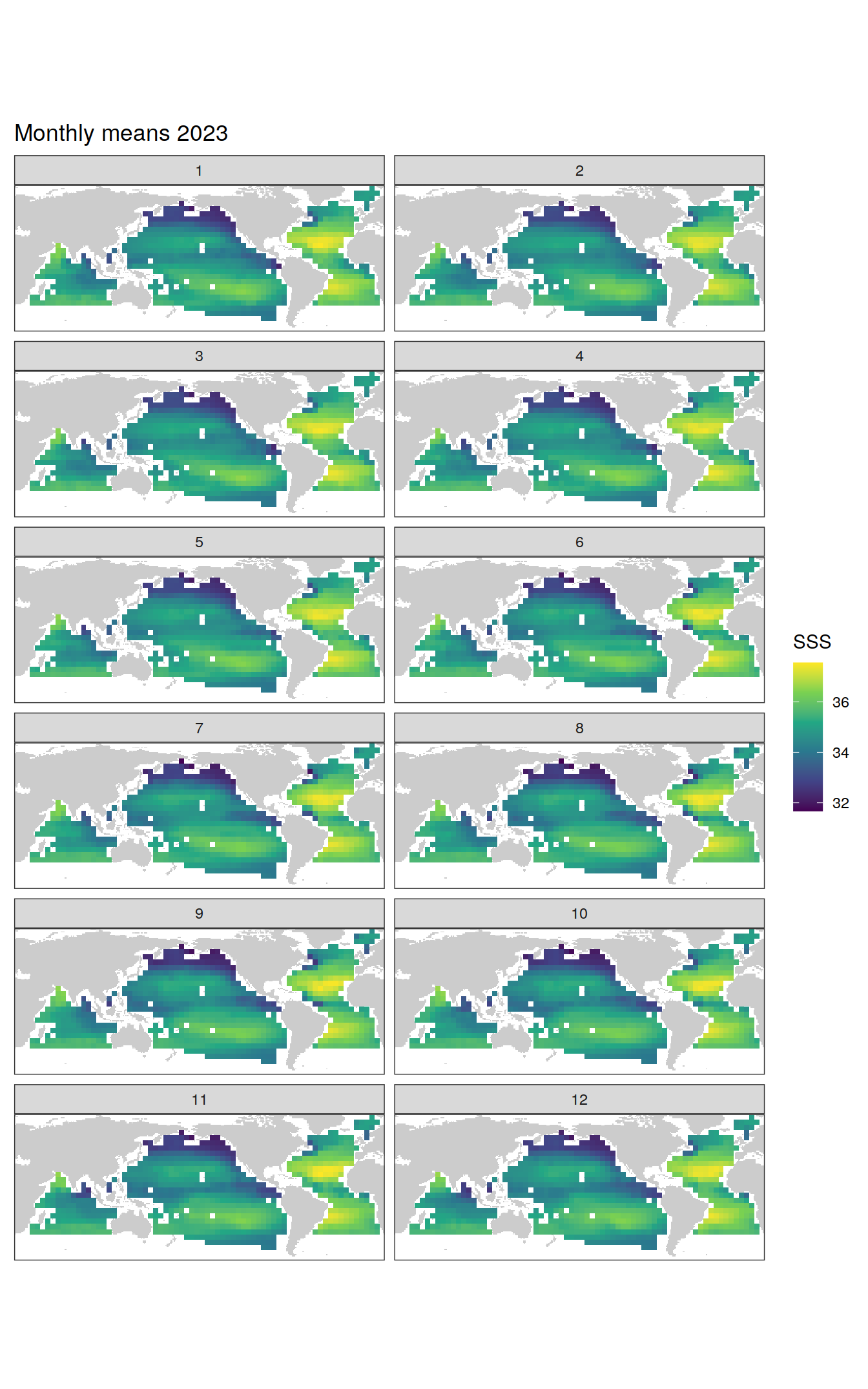
[[6]]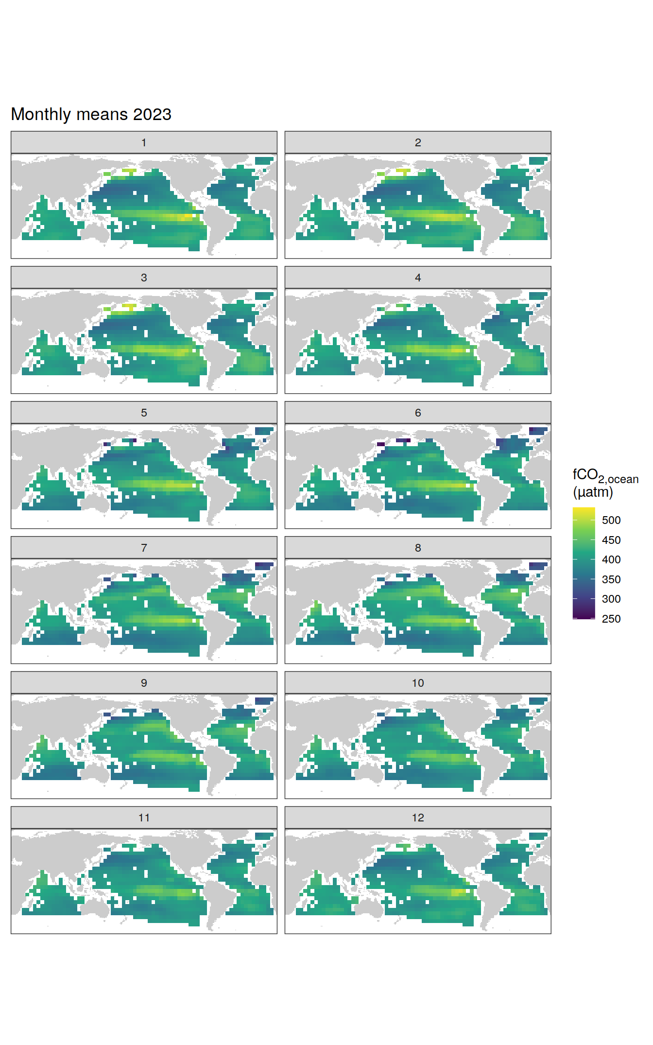
[[7]]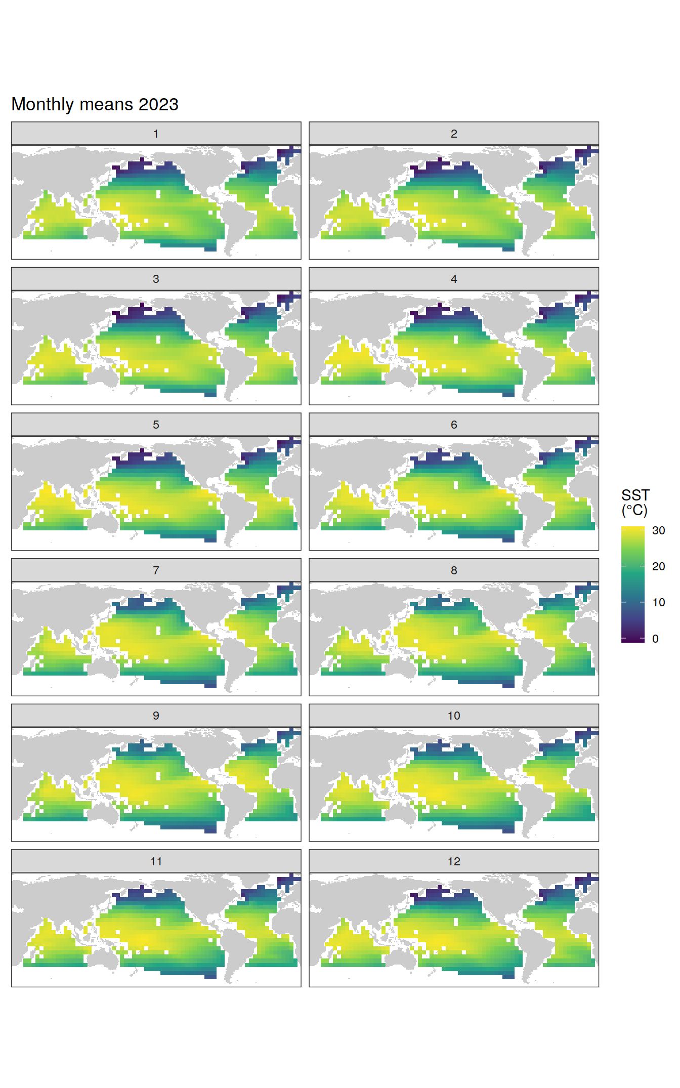
pco2_product_coarse_monthly_regression %>%
  filter(year == 2023,
         name %in% name_divergent) %>%
  group_split(name) %>%
  # head(1) %>%
  map(
    ~ map +
      geom_tile(data = .x,
                aes(lon, lat, fill = value)) +
      labs(title = paste("Monthly means", 2023)) +
      scale_fill_divergent(name = labels_breaks(.x %>% distinct(name))) +
      theme(legend.title = element_markdown()) +
      facet_wrap( ~ month, ncol = 2)
  )
[[1]]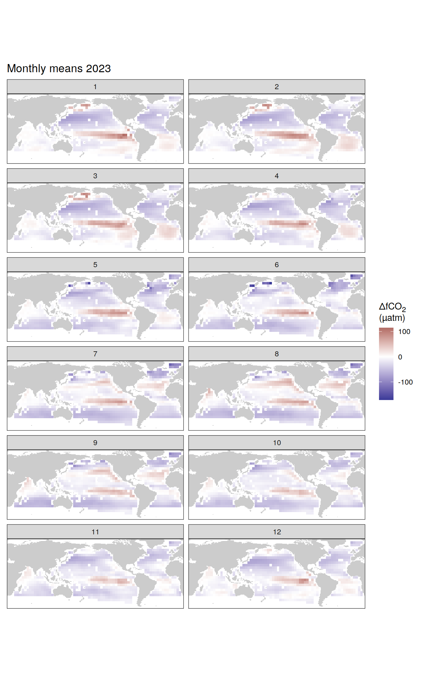
[[2]]
Trends
pco2_product_coarse_monthly_regression %>%
  group_by(name) %>%
  filter(year %in% c(min(year), max(year))) %>%
  ungroup() %>%
  select(-c(value, resid)) %>%
  arrange(year) %>%
  group_by(lon, lat, name, month) %>%
  mutate(change = fit - lag(fit),
         period = paste(lag(year), year, sep = "-")) %>%
  ungroup() %>%
  filter(!is.na(change)) %>%
  group_split(name) %>%
  # head(1) %>%
  map(
    ~ map +
      geom_tile(data = .x,
                aes(lon, lat, fill = change)) +
      labs(title =  paste("Change: ", .x$period)) +
      scale_fill_divergent(name = labels_breaks(.x %>% distinct(name))) +
      theme(legend.title = element_markdown()) +
      facet_wrap(~ month, ncol = 2)
  )
[[1]]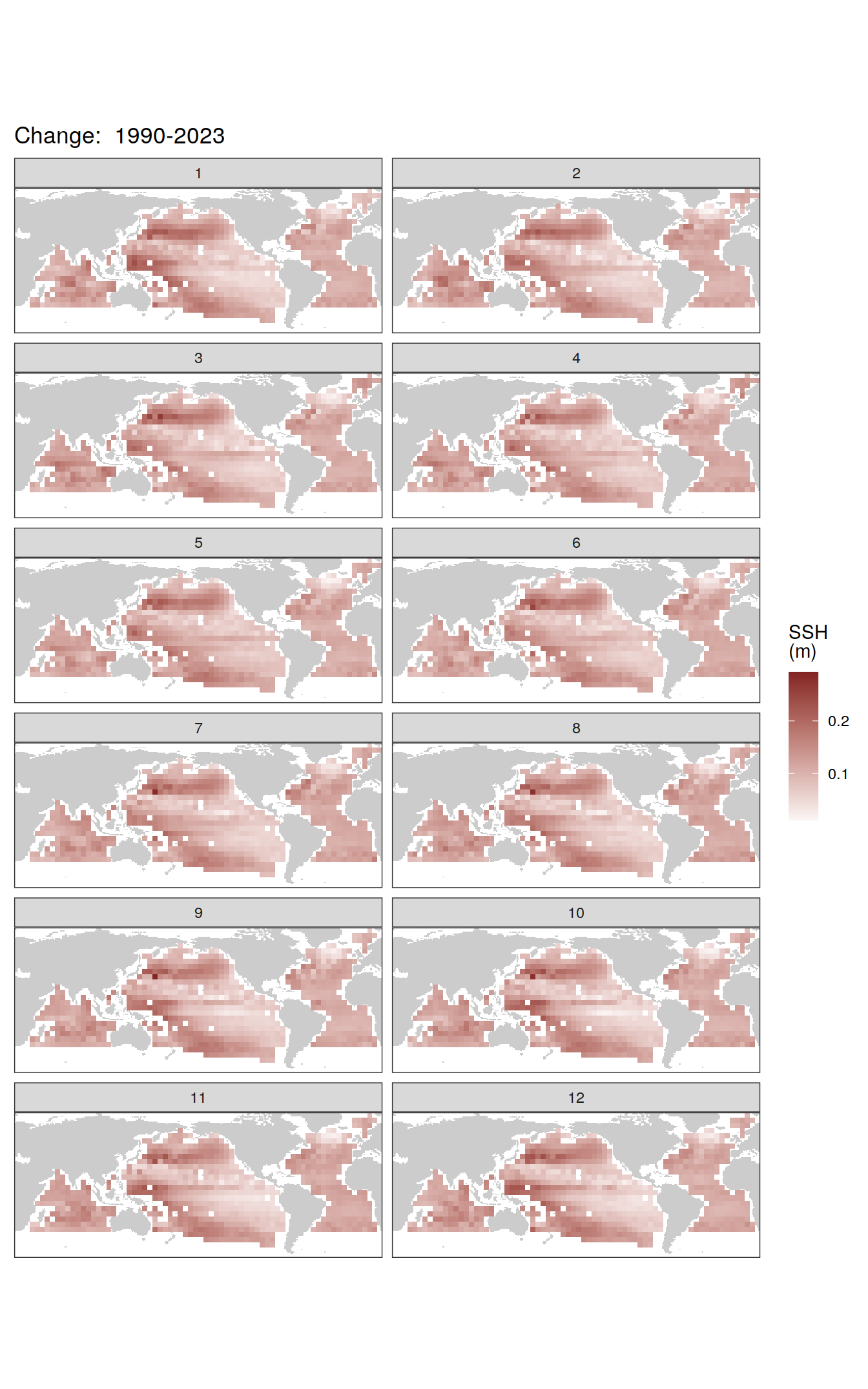
[[2]]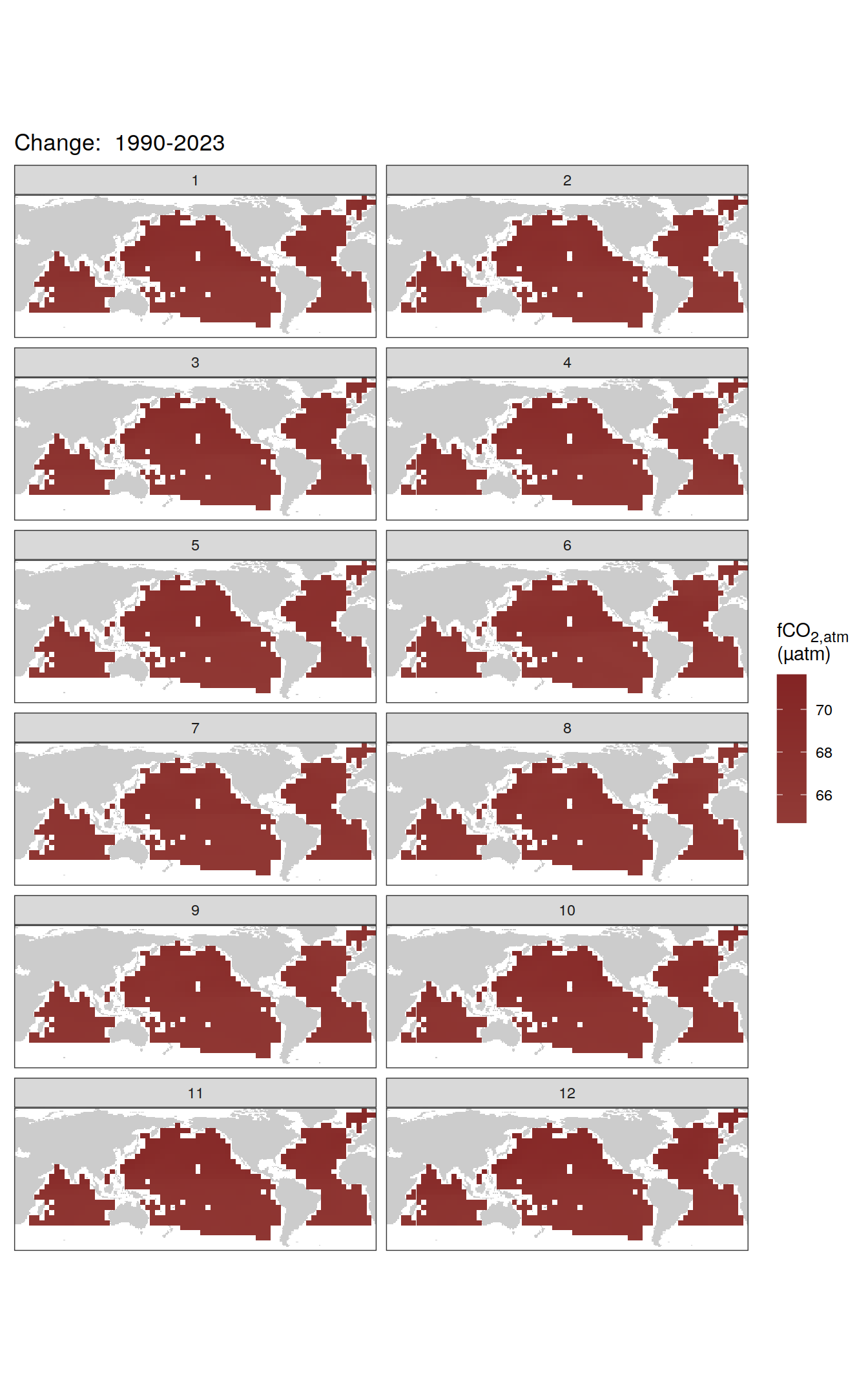
| Version | Author | Date |
|---|---|---|
| 009791f | jens-daniel-mueller | 2024-05-14 |
| 3b5d16b | jens-daniel-mueller | 2024-05-13 |
| 77accd5 | jens-daniel-mueller | 2024-05-07 |
| e9c4ecf | jens-daniel-mueller | 2024-05-07 |
| 5d10d21 | jens-daniel-mueller | 2024-05-07 |
| dfcf790 | jens-daniel-mueller | 2024-04-11 |
| 89becff | jens-daniel-mueller | 2024-04-11 |
| 2321242 | jens-daniel-mueller | 2024-04-11 |
[[3]]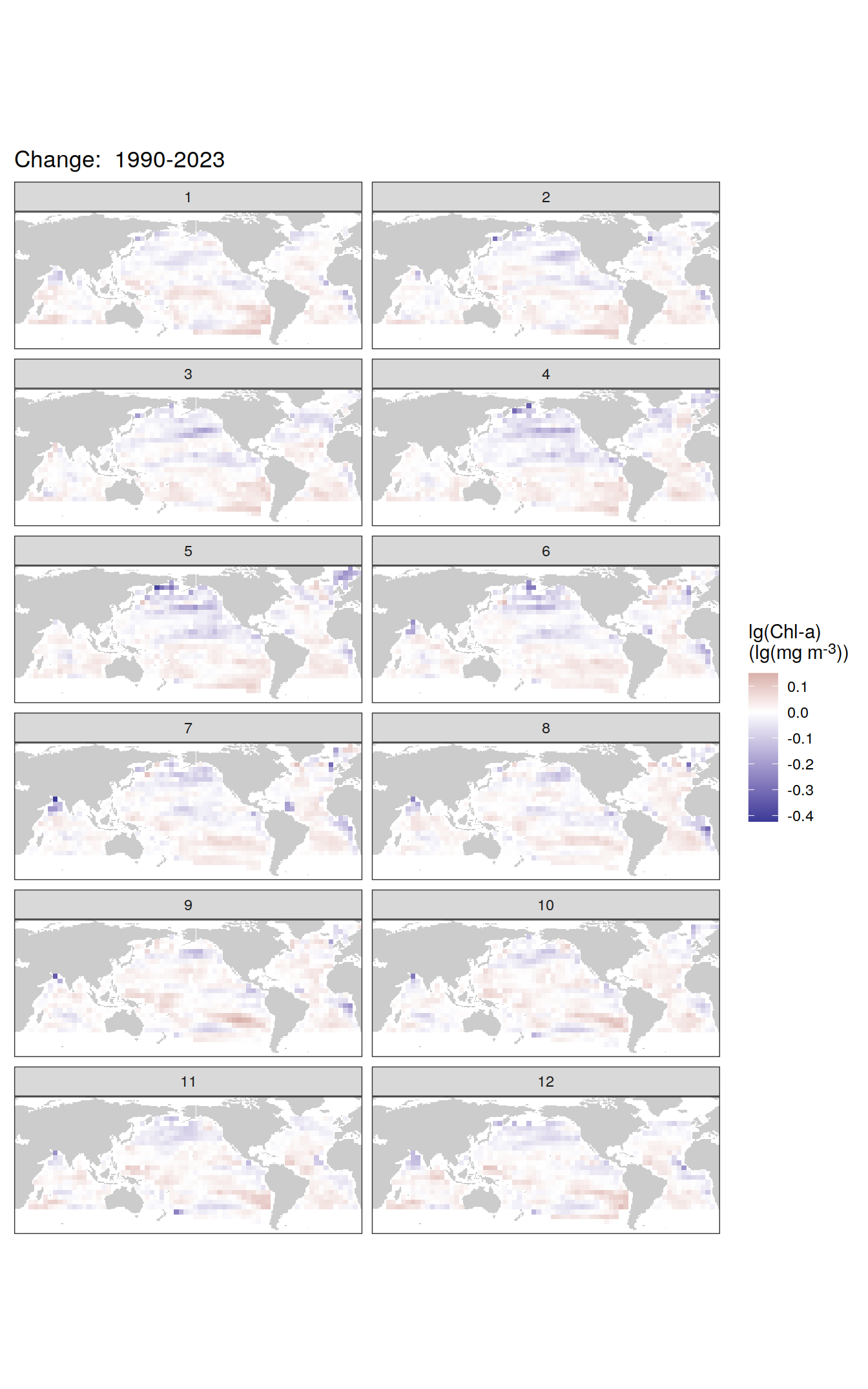
[[4]]
[[5]]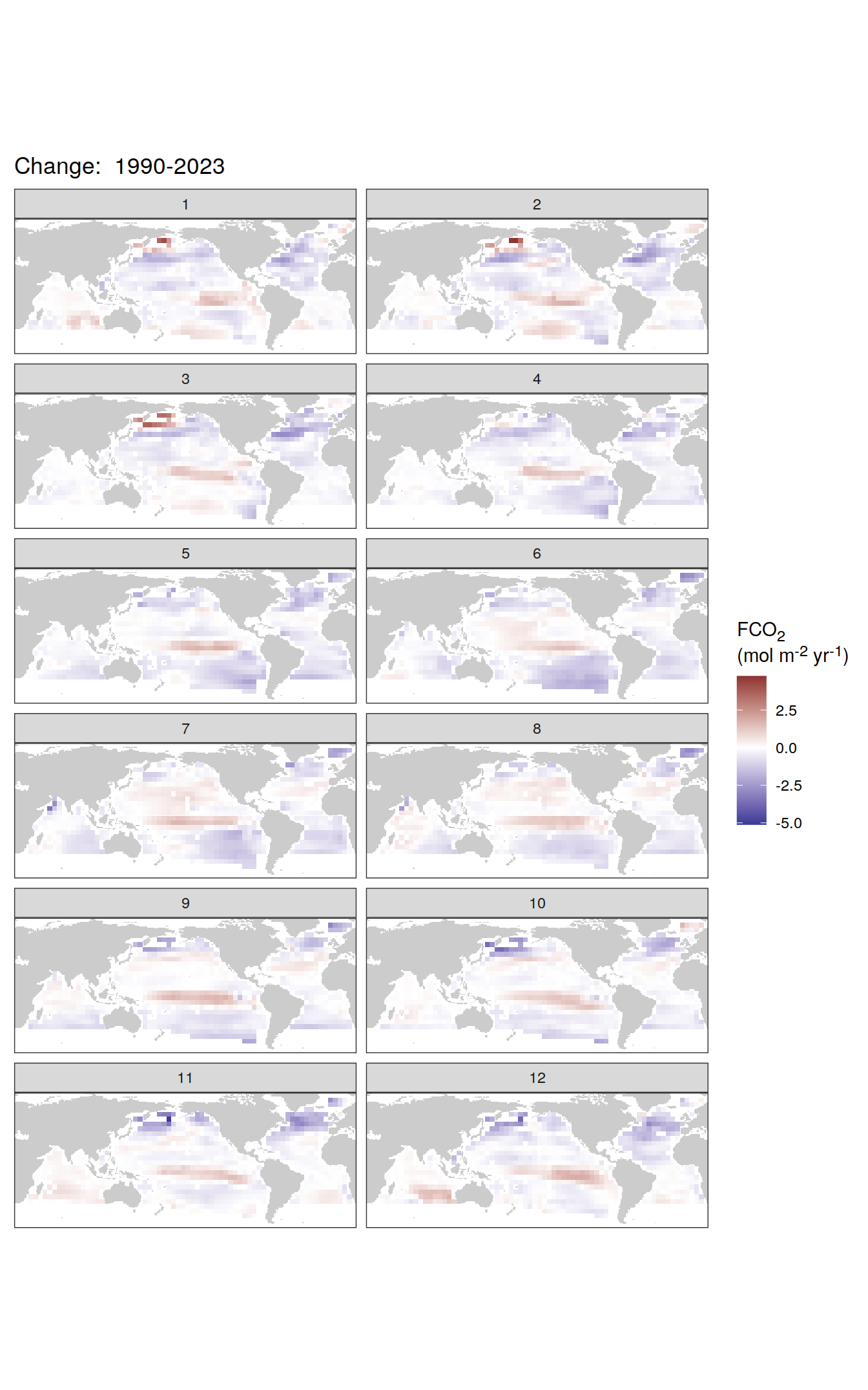
[[6]]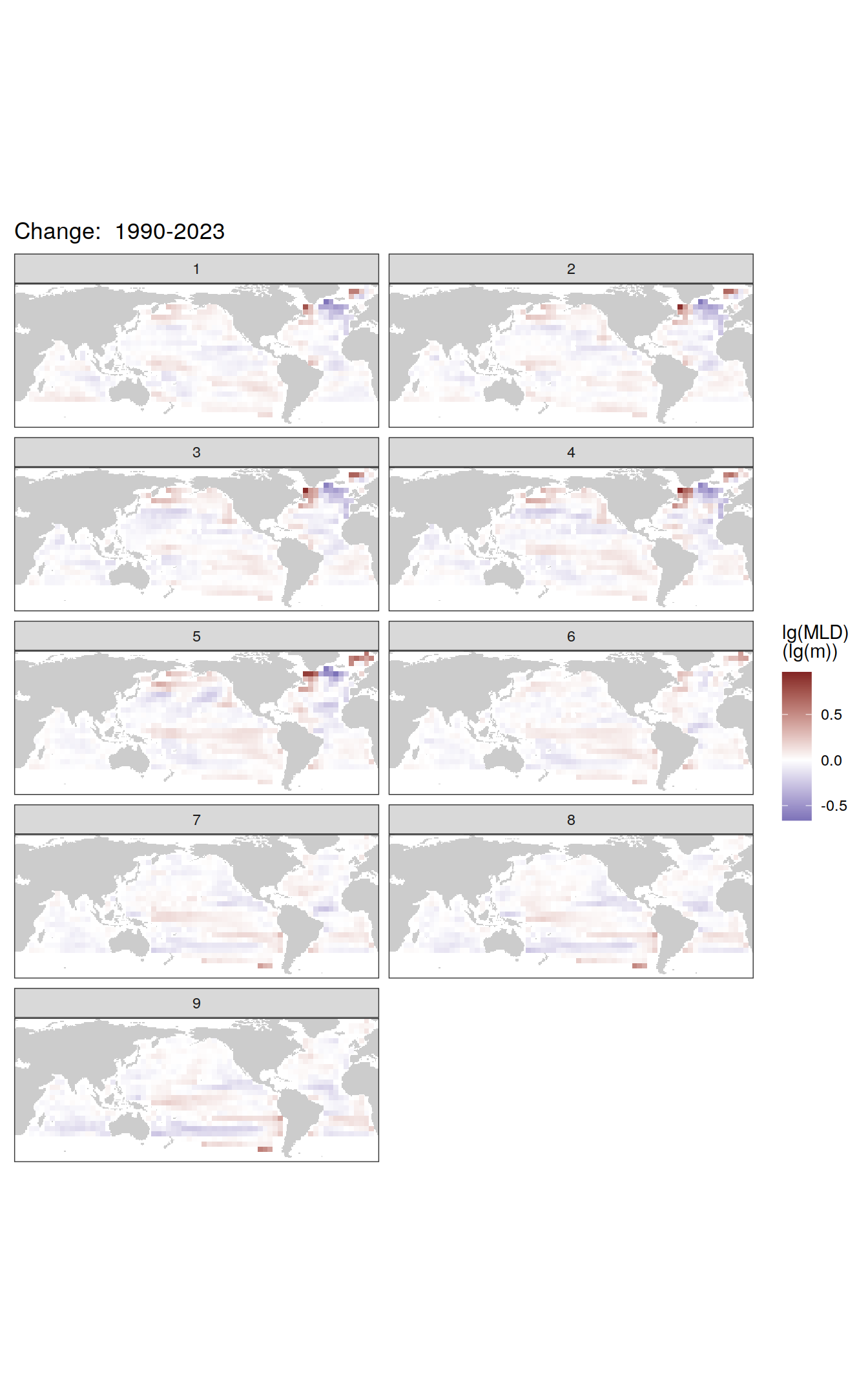
[[7]]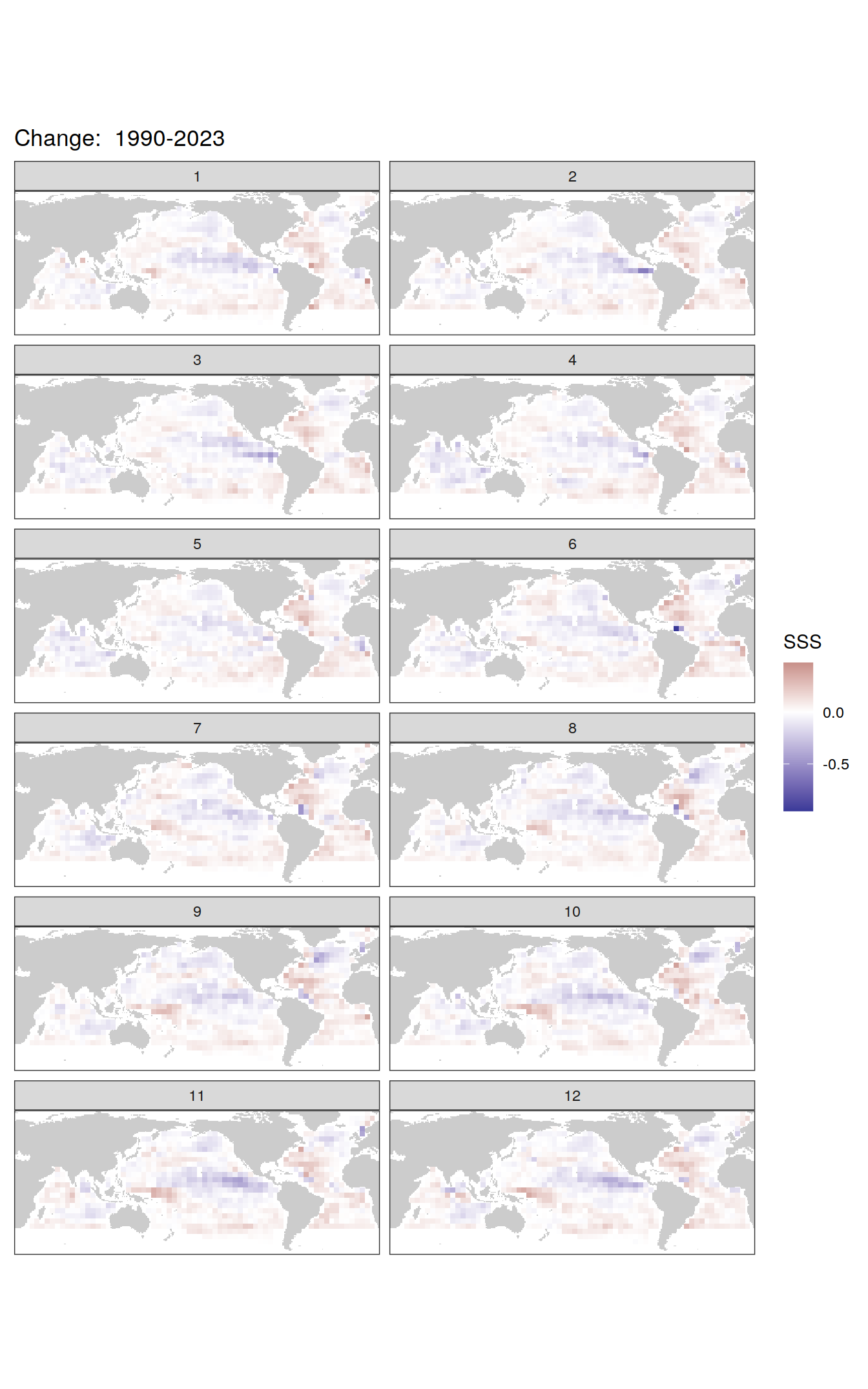
[[8]]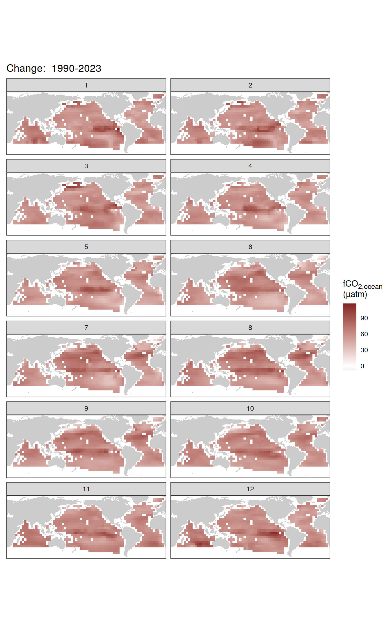
[[9]]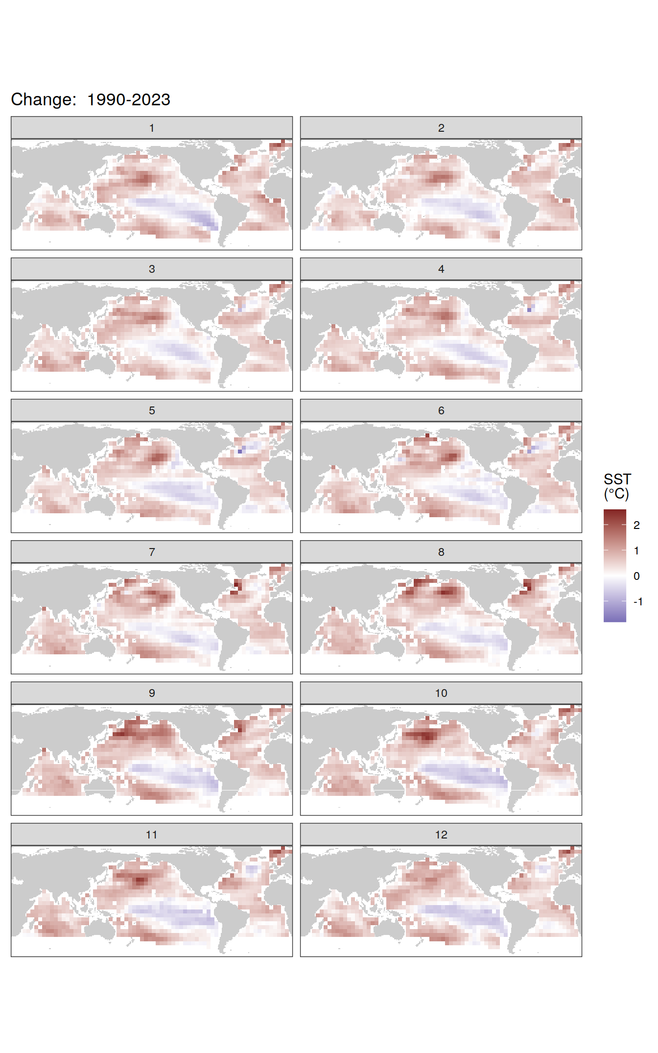
2023 anomaly
pco2_product_coarse_monthly_regression %>%
  filter(year == 2023) %>%
  group_split(name) %>%
  # head(1) %>%
  map(
    ~ map +
      geom_tile(data = .x,
                aes(lon, lat, fill = resid)) +
      labs(title = paste(2023, "anomaly")) +
      scale_fill_divergent(name = labels_breaks(.x %>% distinct(name))) +
      theme(legend.title = element_markdown()) +
      facet_wrap( ~ month, ncol = 2)
  )
[[1]]
[[2]]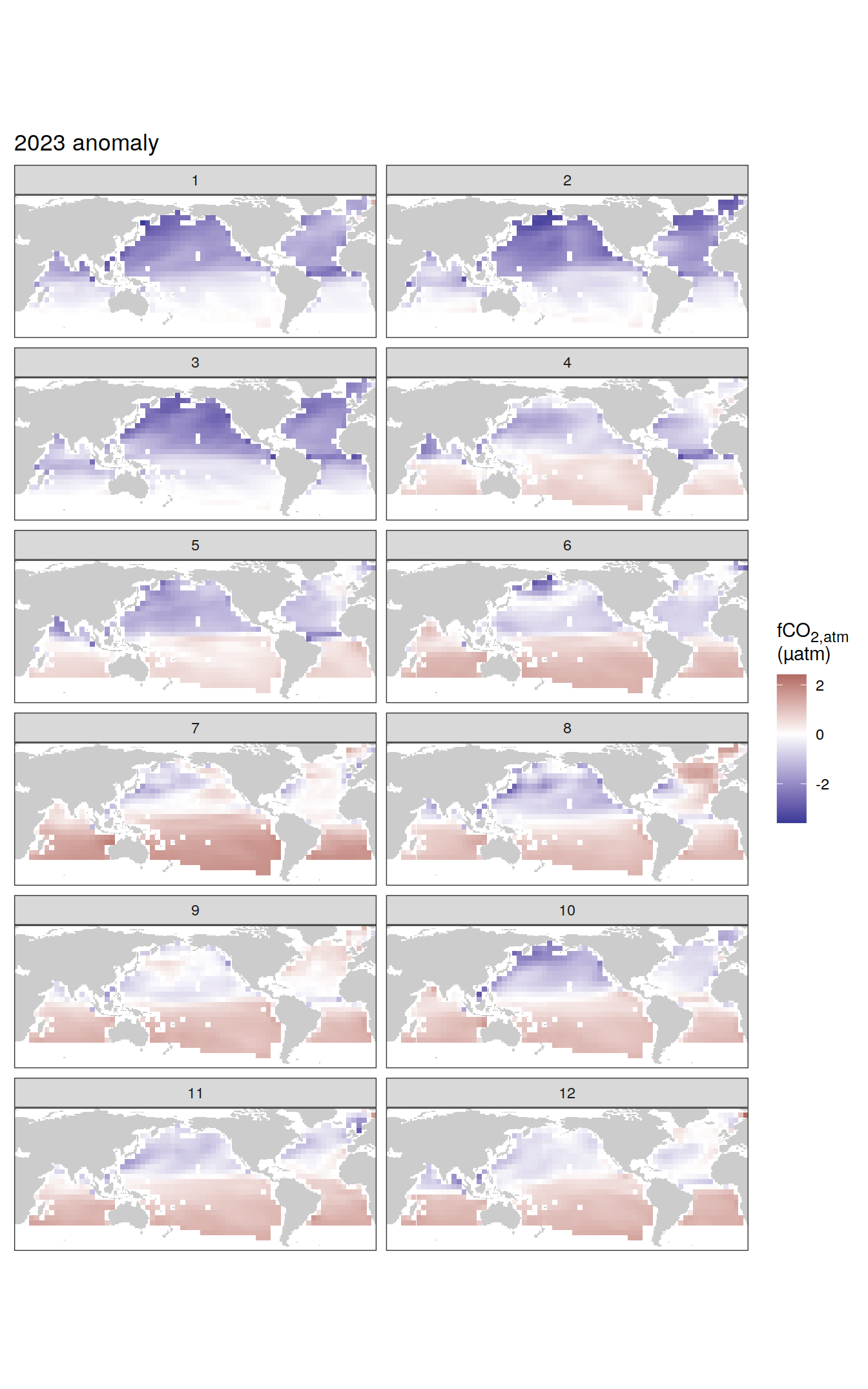
| Version | Author | Date |
|---|---|---|
| 009791f | jens-daniel-mueller | 2024-05-14 |
| 3b5d16b | jens-daniel-mueller | 2024-05-13 |
| 77accd5 | jens-daniel-mueller | 2024-05-07 |
| e9c4ecf | jens-daniel-mueller | 2024-05-07 |
| 5d10d21 | jens-daniel-mueller | 2024-05-07 |
| dfcf790 | jens-daniel-mueller | 2024-04-11 |
| 89becff | jens-daniel-mueller | 2024-04-11 |
| 2321242 | jens-daniel-mueller | 2024-04-11 |
[[3]]
[[4]]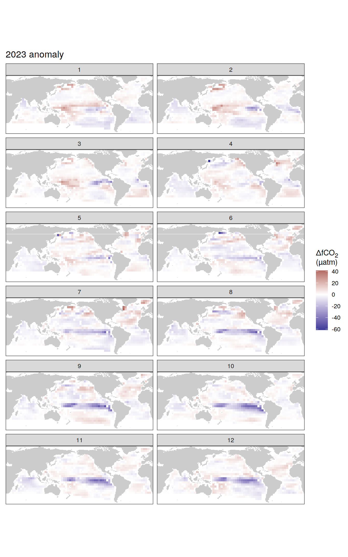
[[5]]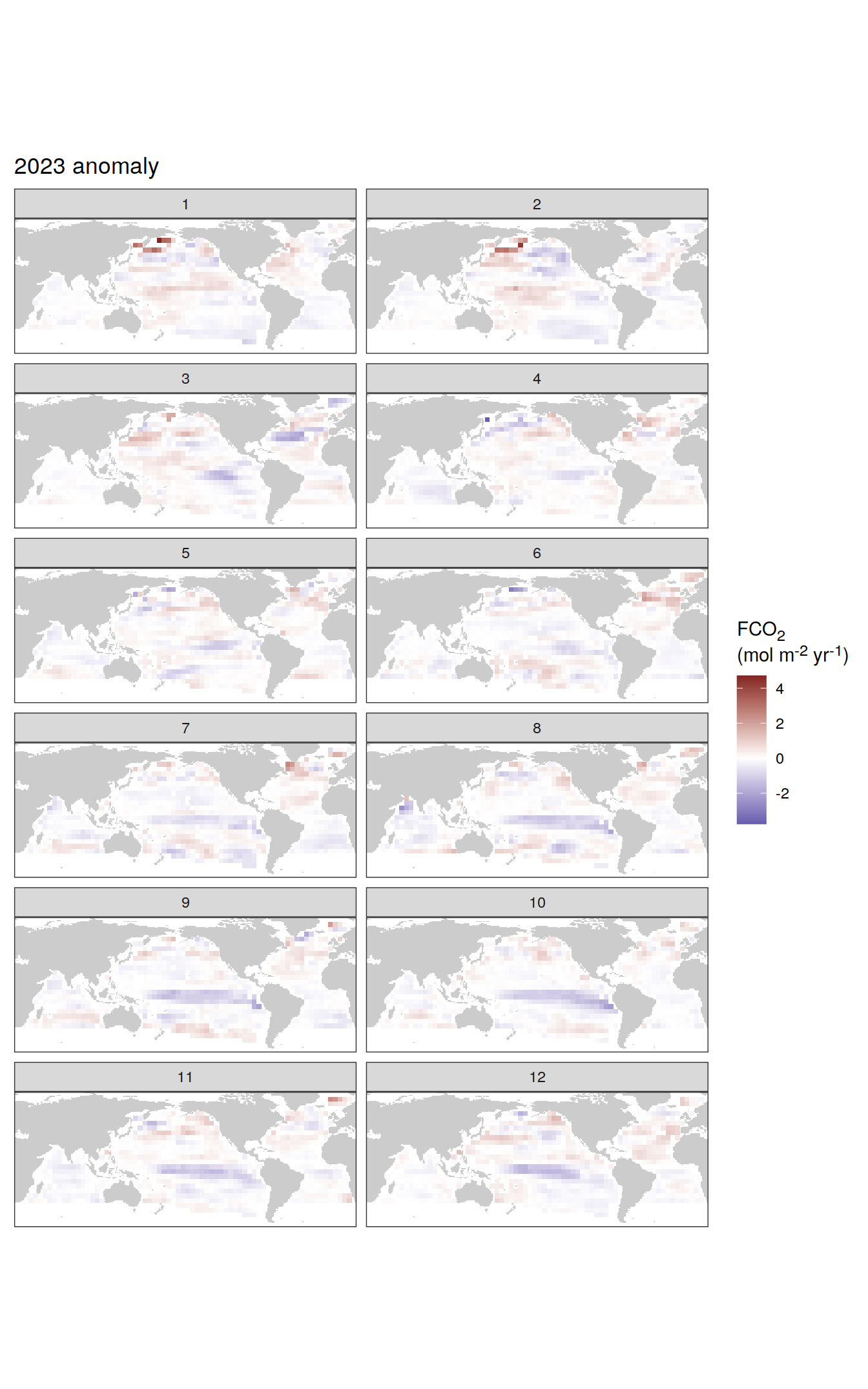
[[6]]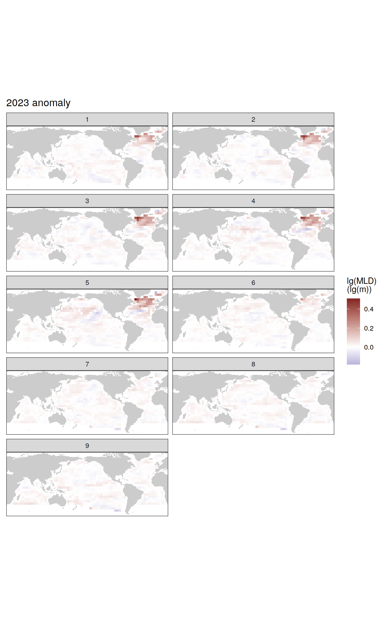
[[7]]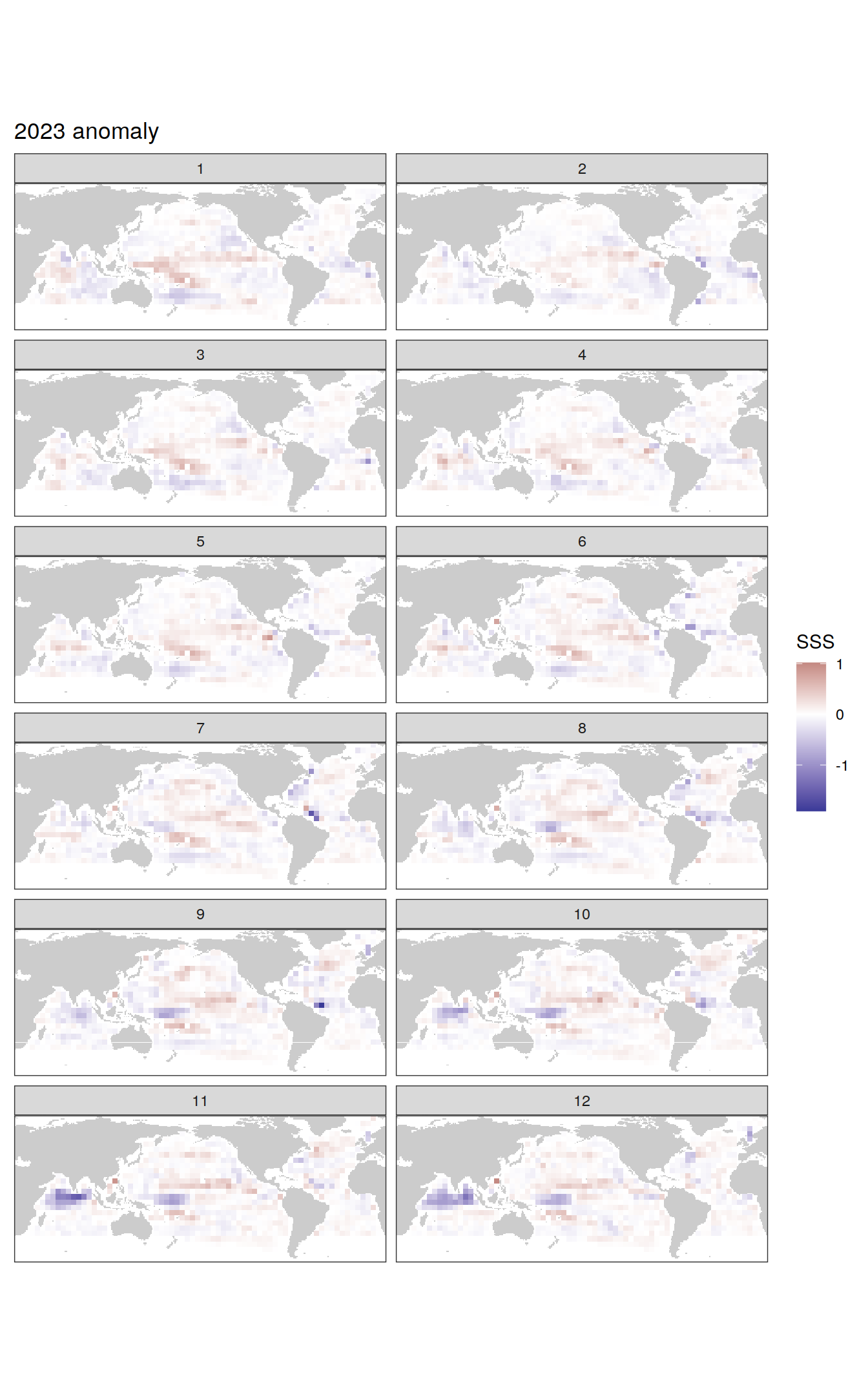
[[8]]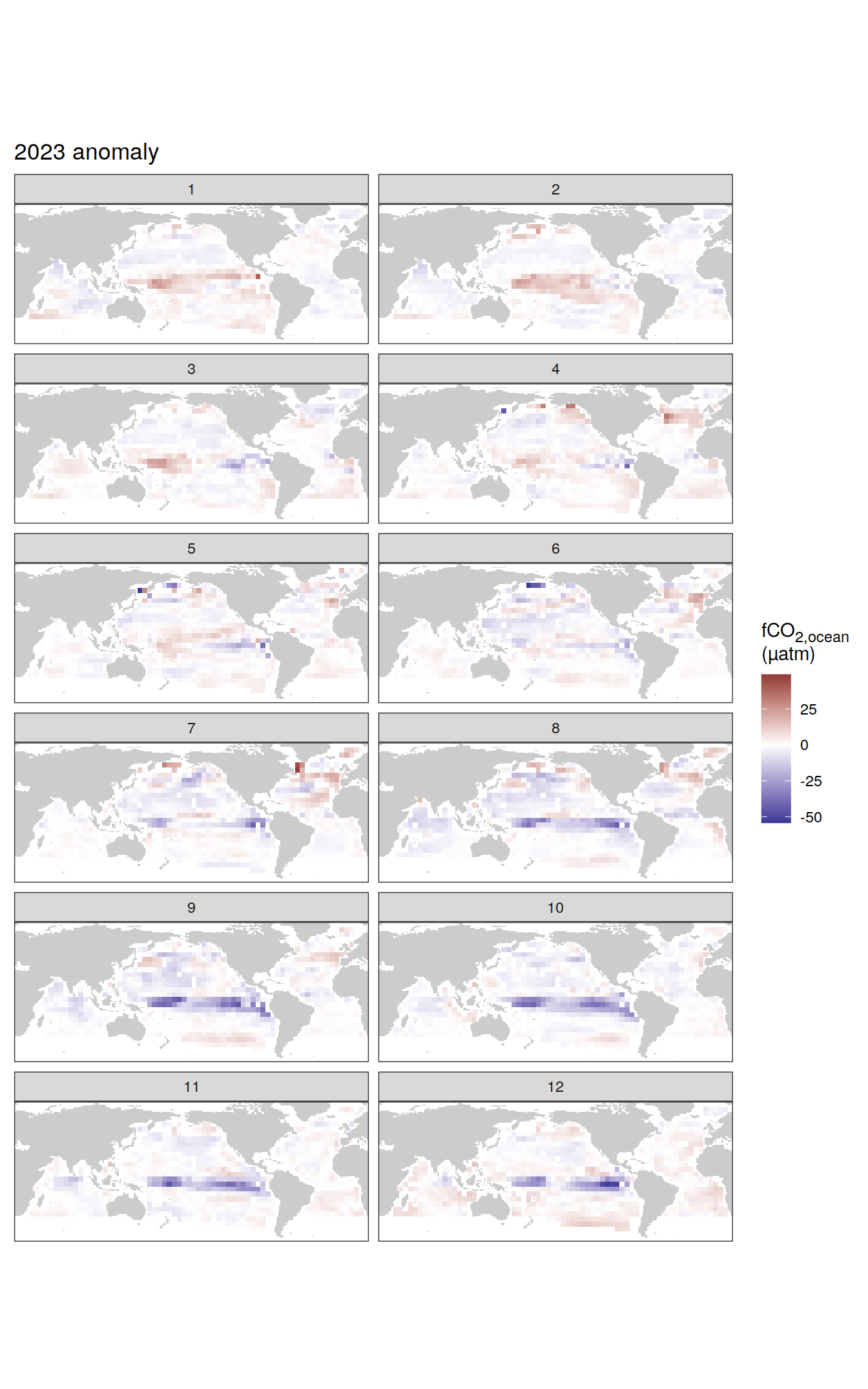
[[9]]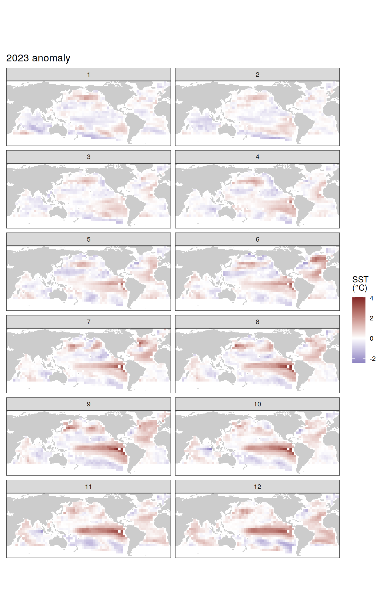
pco2_product_coarse_monthly_regression %>%
  filter(year == 2023) %>%
  write_csv(paste0("../data/","CMEMS","_","2023","_anomaly_map_monthly.csv"))
Hovmoeller plots
The following Hovmoeller plots show the anomalies from the prediction of the linear/quadratic fits.
Hovmoeller plots are first presented as annual means, and than as monthly means. Note that the predictions for the monthly Hovmoeller plots are done individually for each month, such the mean seasonal anomaly from the annual mean is removed.
2023 annual anomalies
pco2_product_hovmoeller_monthly_annual_regression <-
  pco2_product_hovmoeller_monthly_annual %>%
  anomaly_determination(lat) %>%
  filter(!is.na(resid))


pco2_product_hovmoeller_monthly_annual_regression %>%
  # filter(name == "mld") %>%
  group_split(name) %>%
  # head(1) %>%
  map(
    ~ ggplot(data = .x,
             aes(year, lat, fill = resid)) +
      geom_raster() +
      scale_fill_divergent(name = labels_breaks(.x %>% distinct(name))) +
      theme(legend.title = element_markdown()) +
      coord_cartesian(expand = 0) +
      labs(title = "Annual mean anomalies",
           y = "Latitude") +
      theme(axis.title.x = element_blank())
  )
[[1]]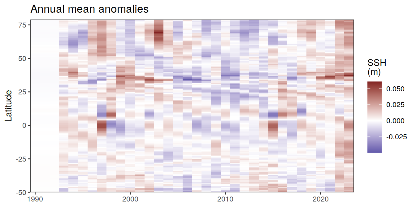
[[2]]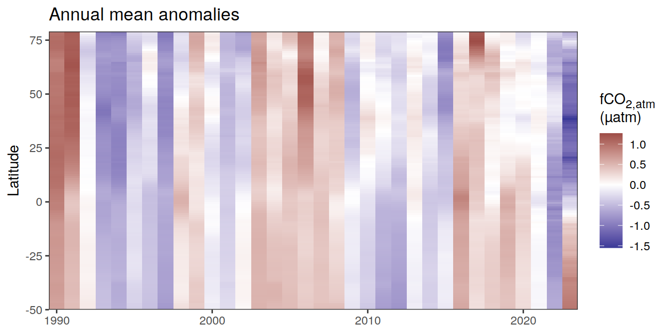
[[3]]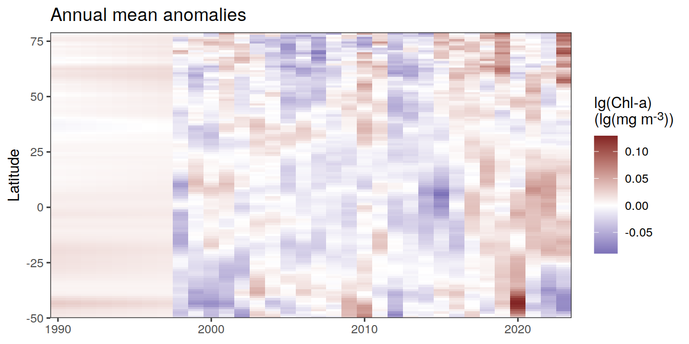
[[4]]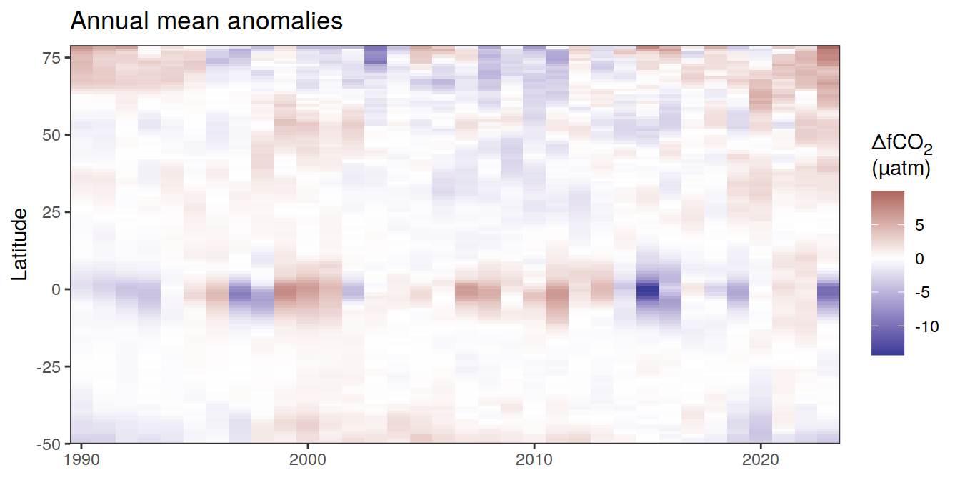
[[5]]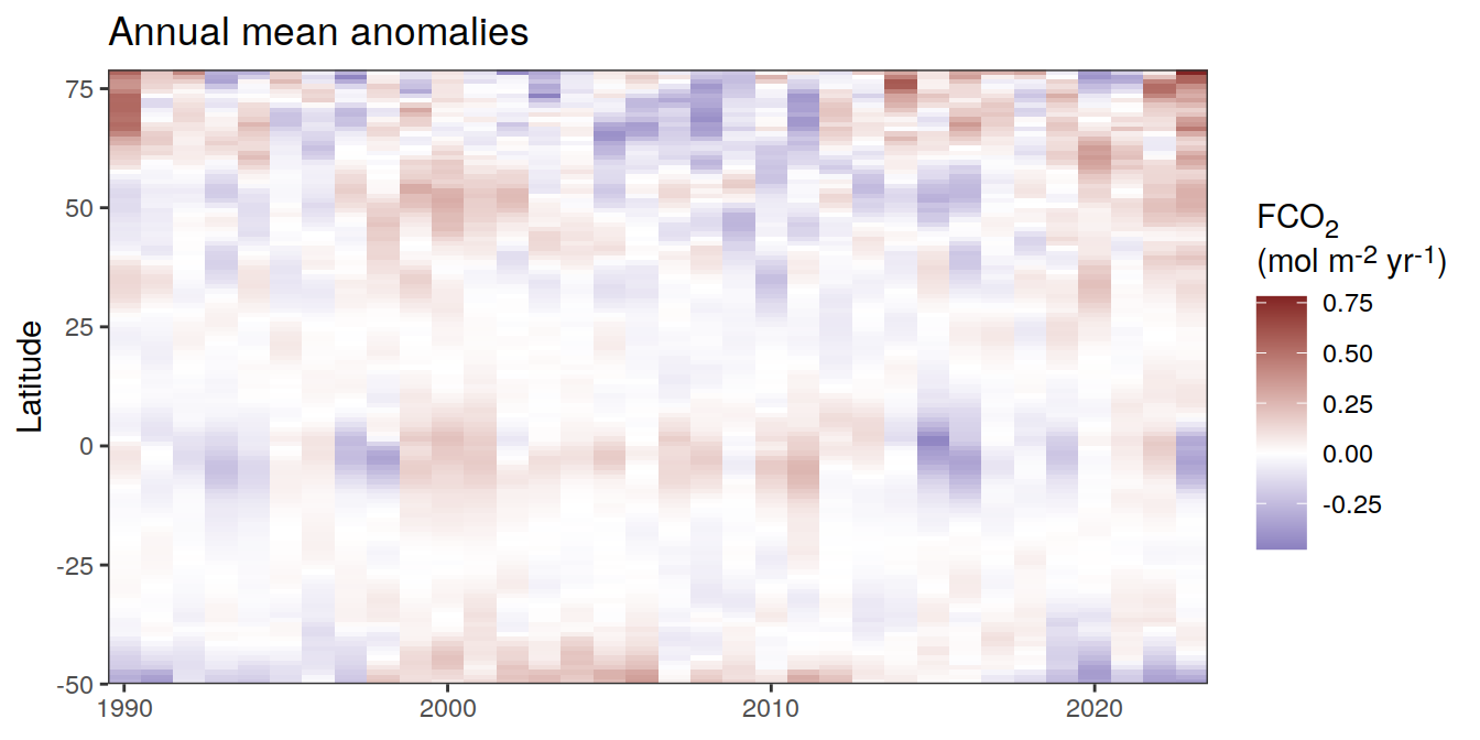
[[6]]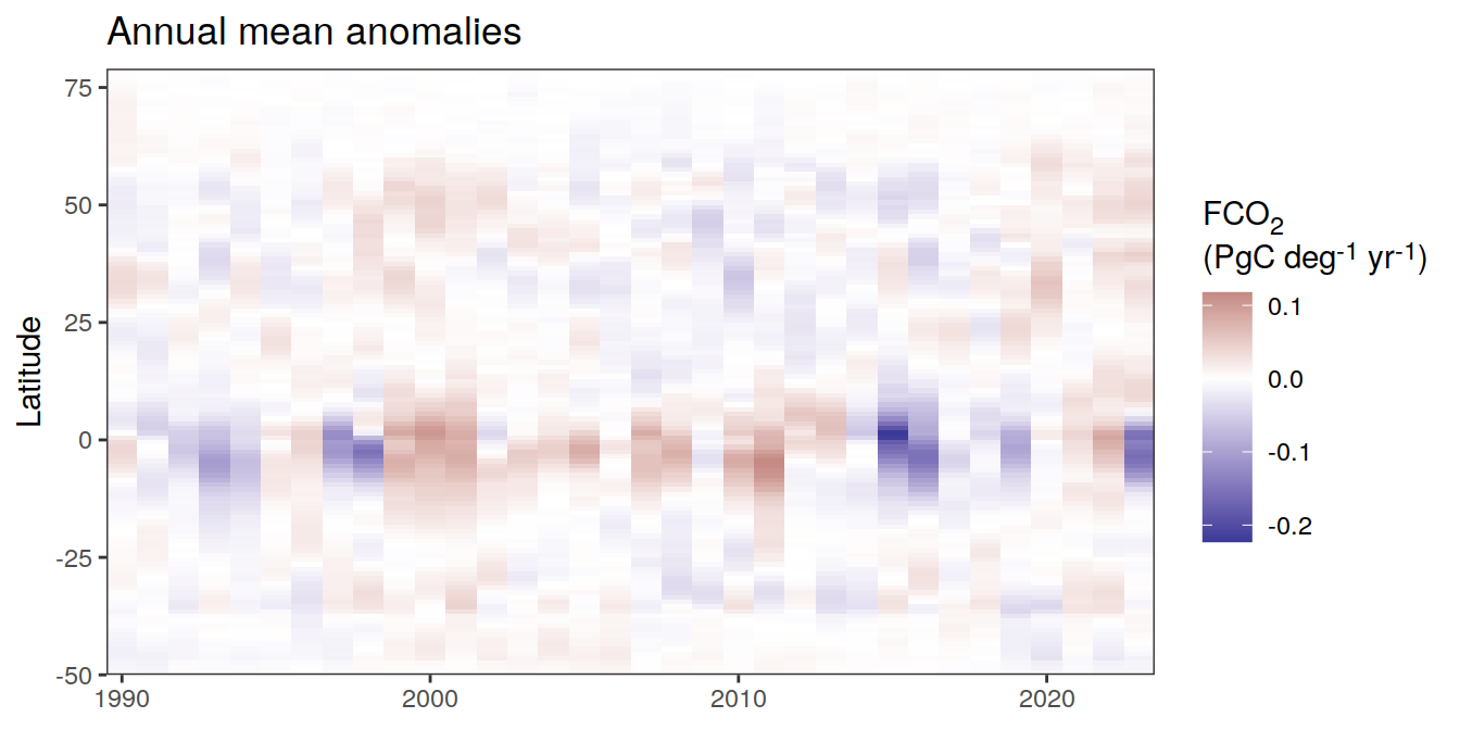
[[7]]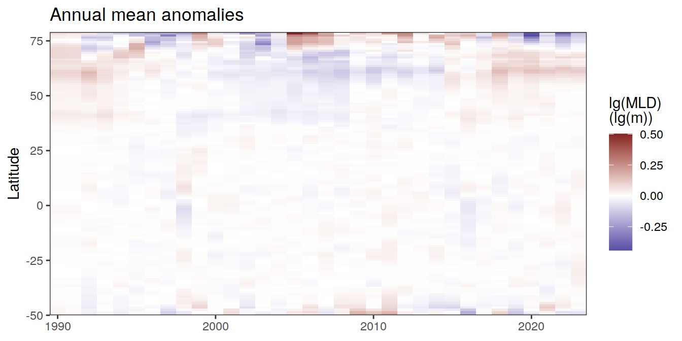
[[8]]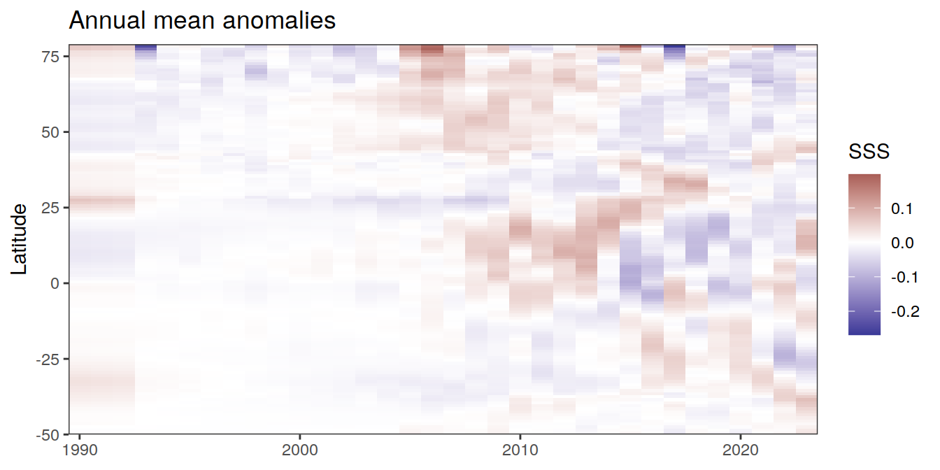
[[9]]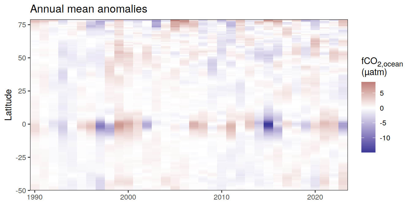
[[10]]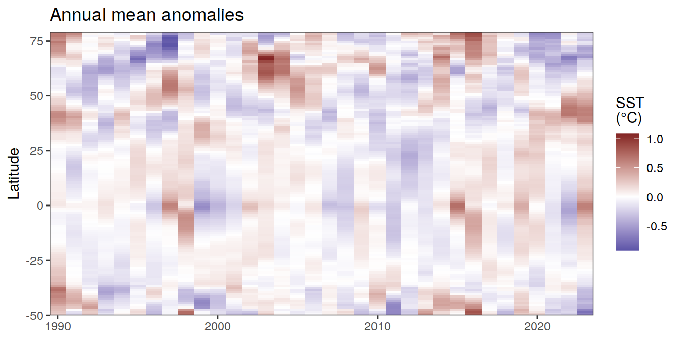
2023 monthly anomalies
pco2_product_hovmoeller_monthly_regression <-
  pco2_product_hovmoeller_monthly %>%
  select(-c(decimal)) %>%
  anomaly_determination(lat, month) %>%
  filter(!is.na(resid))


pco2_product_hovmoeller_monthly_regression <-
  pco2_product_hovmoeller_monthly_regression %>%
  mutate(decimal = year + (month - 1) / 12)

pco2_product_hovmoeller_monthly_regression %>%
  group_split(name) %>%
  # head(1) %>%
  map(
    ~ ggplot(data = .x,
             aes(decimal, lat, fill = resid)) +
      geom_raster() +
      scale_fill_divergent(name = labels_breaks(.x %>% distinct(name))) +
      theme(legend.title = element_markdown()) +
      coord_cartesian(expand = 0) +
      labs(title = "Monthly mean anomalies",
           y = "Latitude") +
      theme(axis.title.x = element_blank())
  )
[[1]]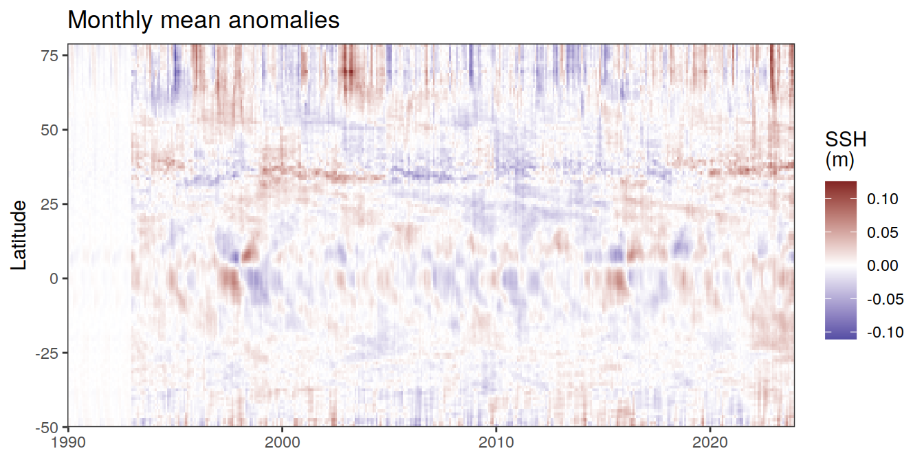
[[2]]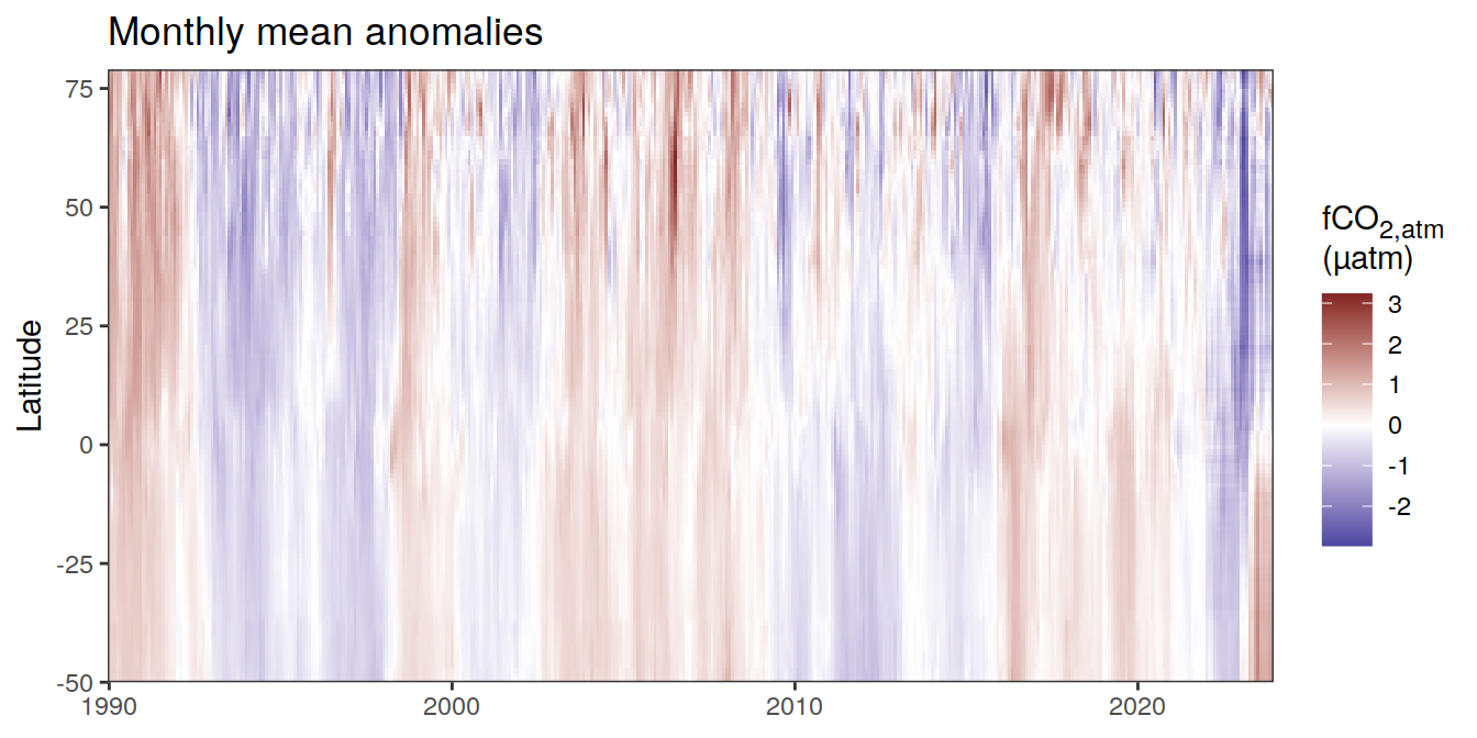
[[3]]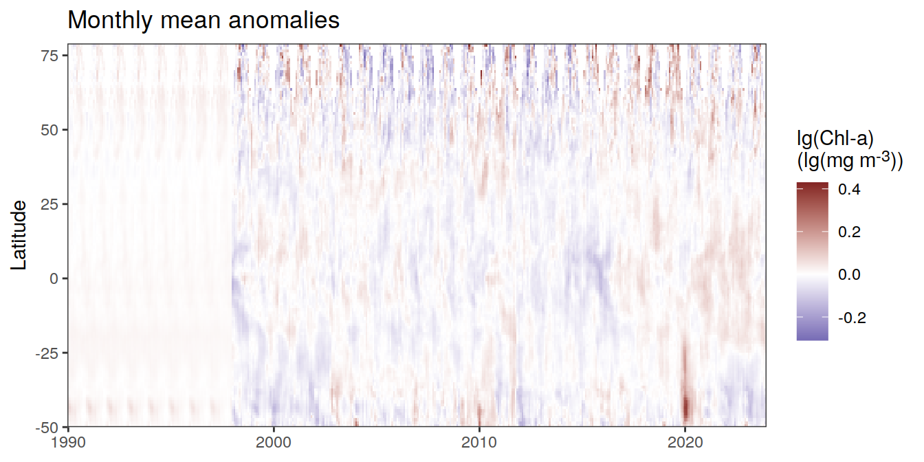
[[4]]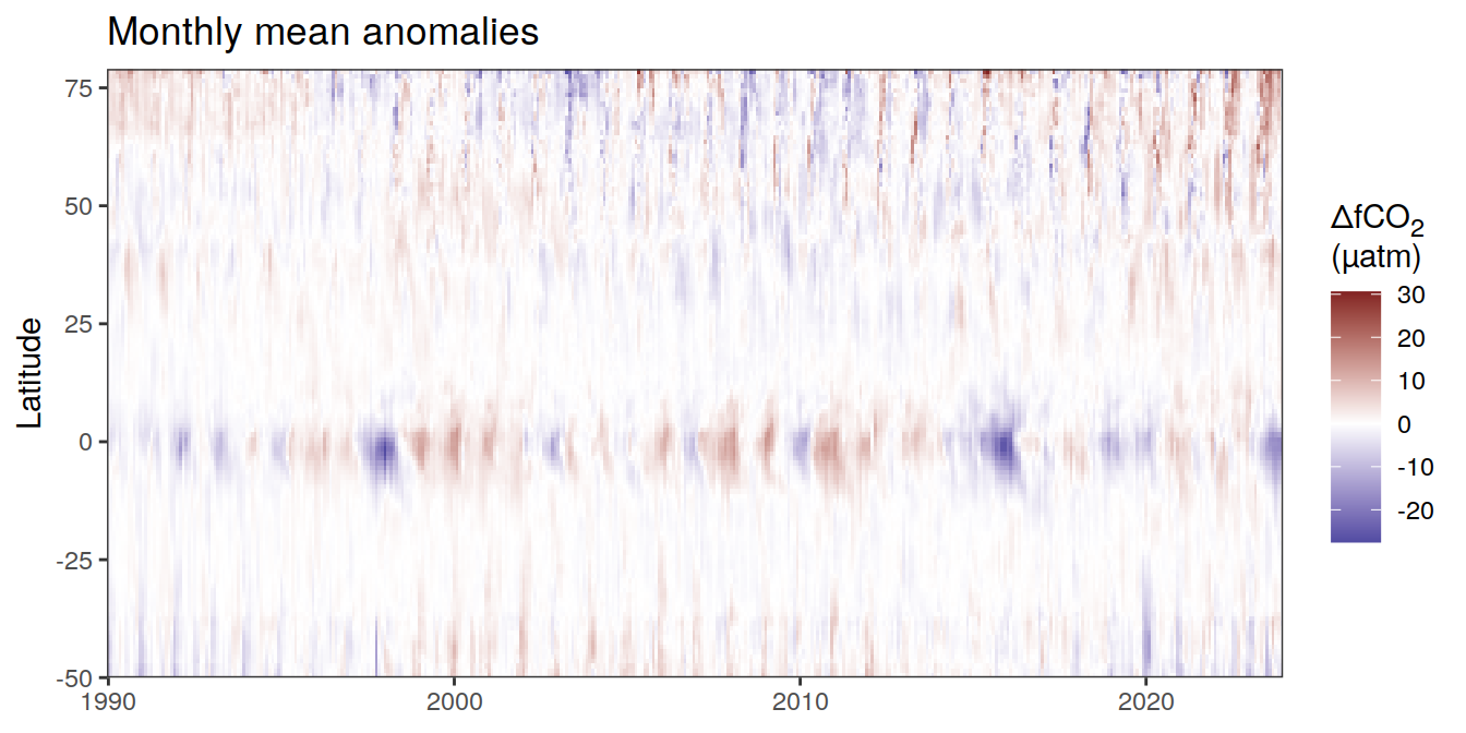
[[5]]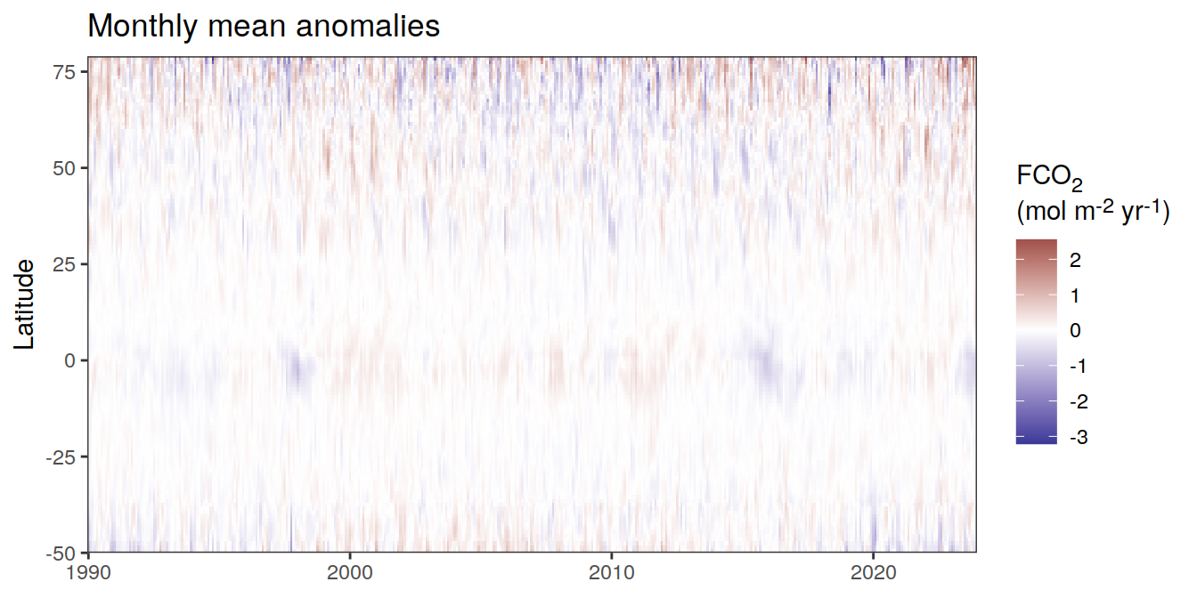
[[6]]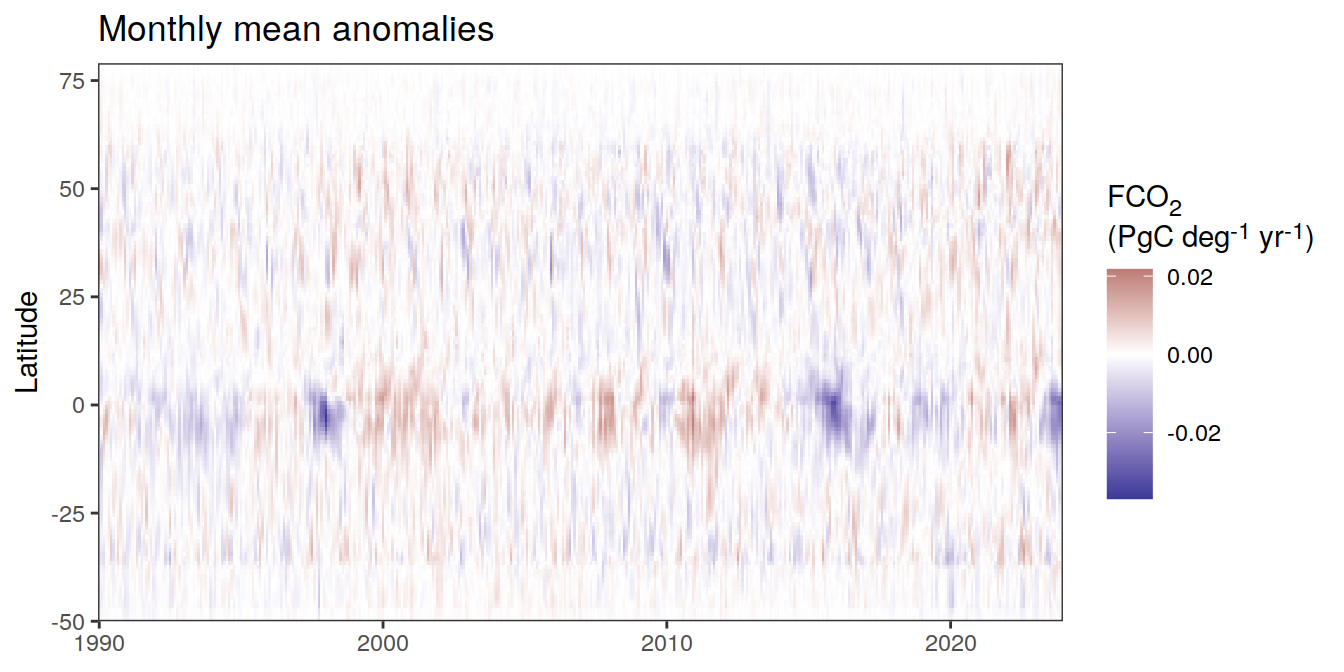
[[7]]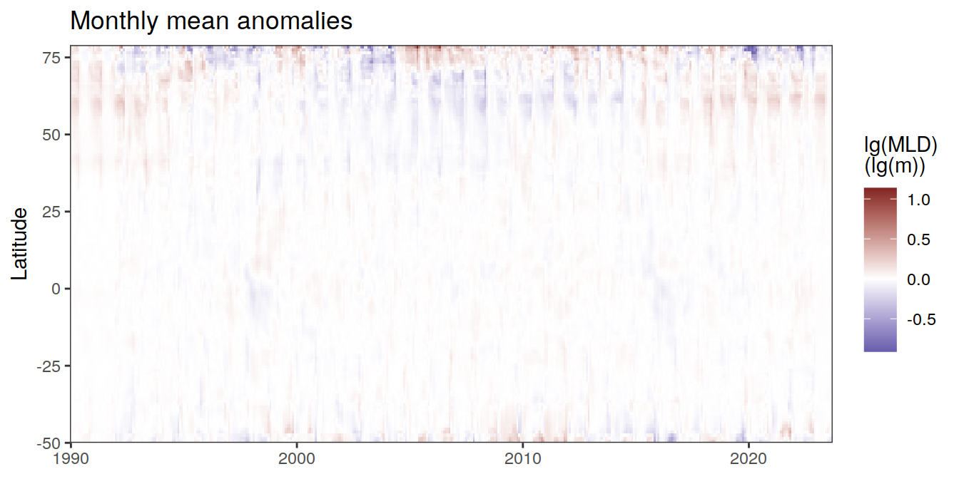
[[8]]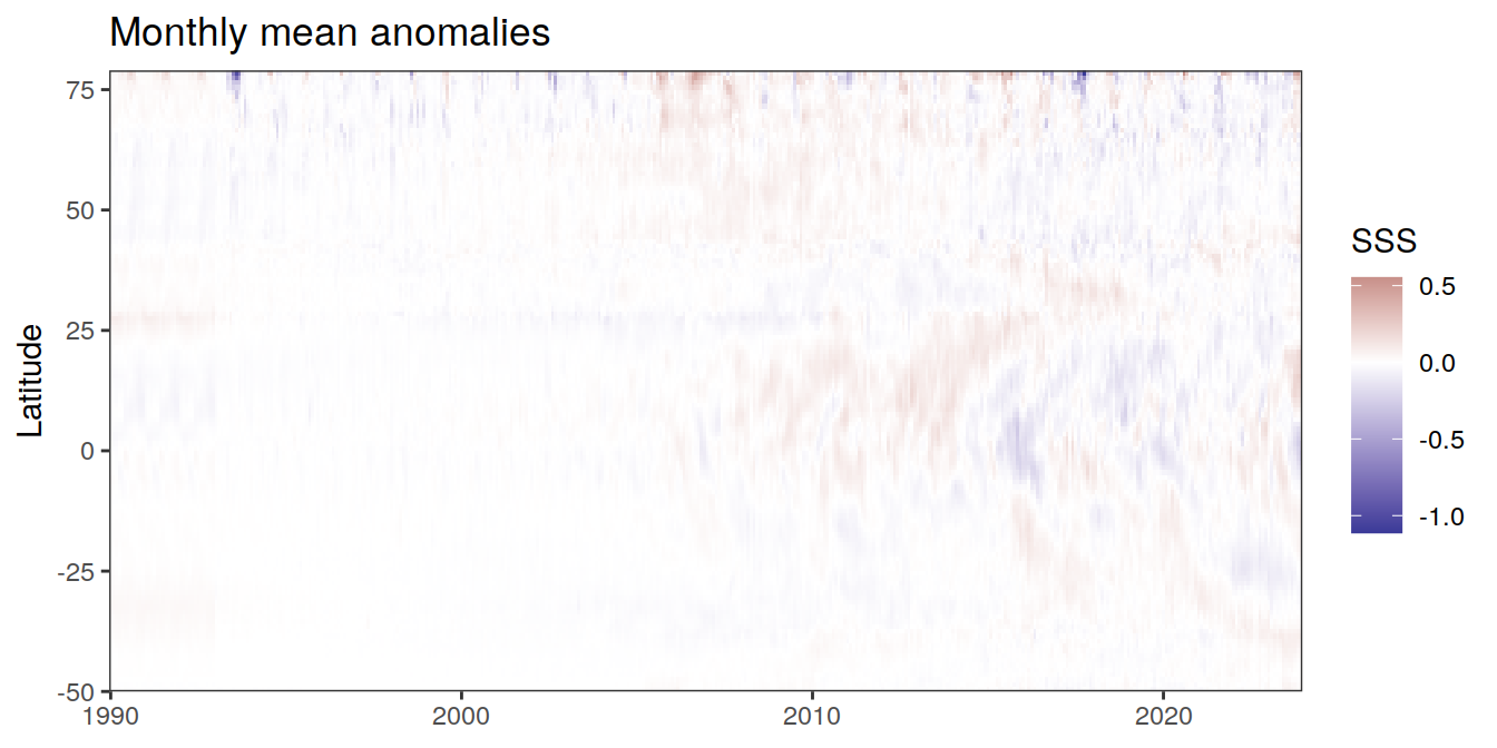
[[9]]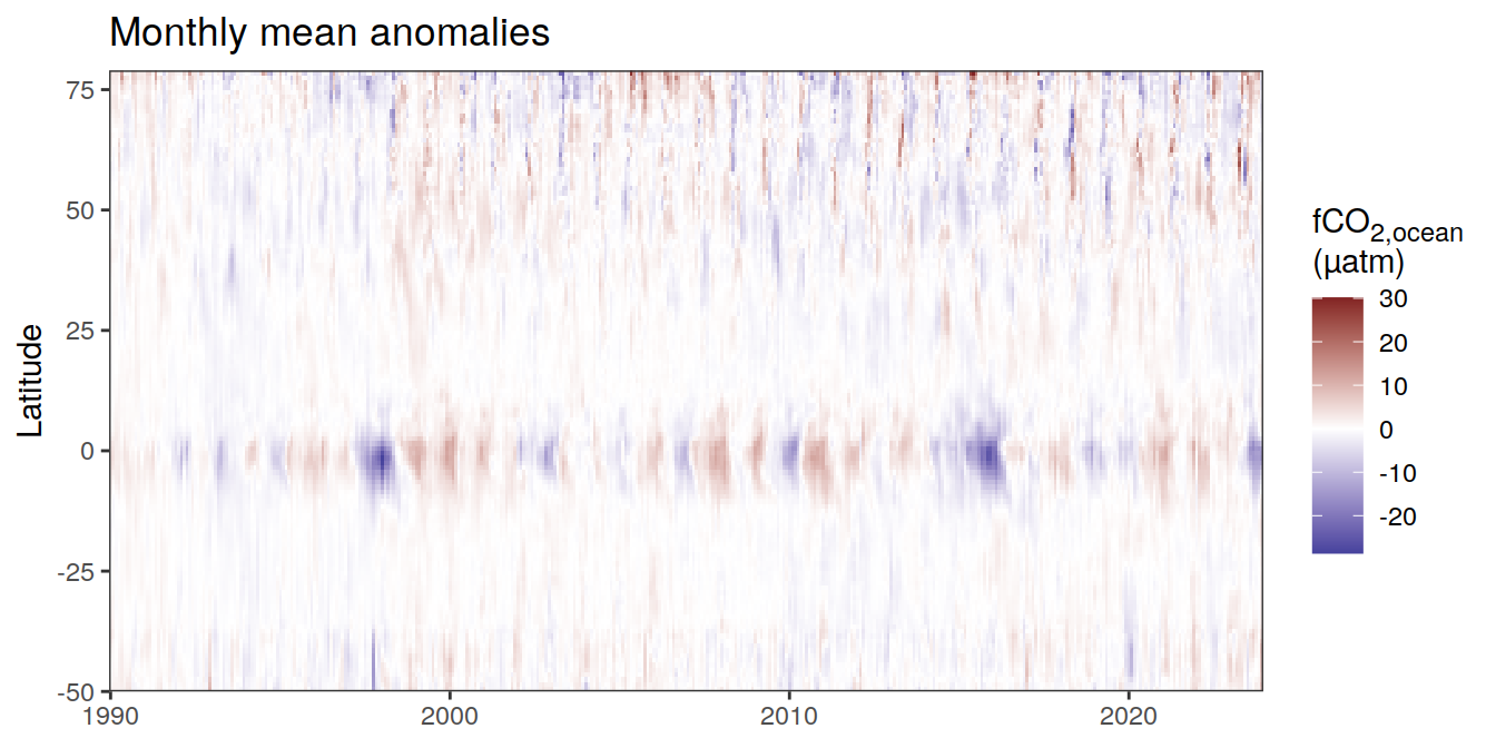
[[10]]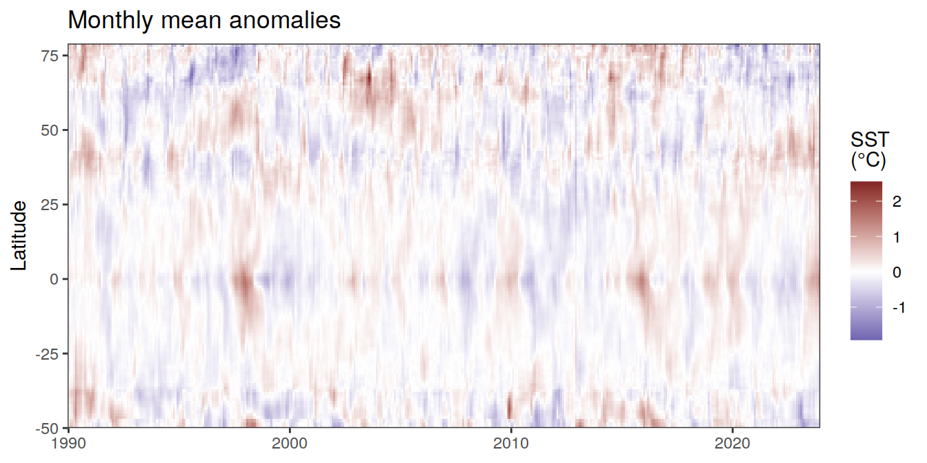
pco2_product_hovmoeller_monthly_regression %>%
  write_csv(paste0("../data/","CMEMS","_","2023","_anomaly_hovmoeller_monthly.csv"))
Three years prior 2023
pco2_product_hovmoeller_monthly_regression %>%
  filter(between(year, 2023-2, 2023)) %>%
  group_split(name) %>%
  # head(1) %>%
  map(
    ~ ggplot(data = .x,
             aes(decimal, lat, fill = resid)) +
      geom_raster() +
      scale_fill_divergent(name = labels_breaks(.x %>% distinct(name))) +
      theme(legend.title = element_markdown()) +
      coord_cartesian(expand = 0) +
      labs(title = "Monthly mean anomalies",
           y = "Latitude") +
      theme(axis.title.x = element_blank())
  )
[[1]]
[[2]]
[[3]]
[[4]]
[[5]]
[[6]]
[[7]]
[[8]]
[[9]]
[[10]]
Regional means and integrals
The following plots show regionally averaged (or integrated) values of each variable as provided through the pCO2 product, as well as the anomalies from the prediction of a linear/quadratic fit.
Anomalies are first presented relative to the predicted annual mean of each year, hence preserving the seasonality. Furthermore, anomalies are presented relative to the predicted monthly mean values, such that the mean seasonality is removed.
2023 absolute values
Global
fig.height <- pco2_product_monthly %>%
  distinct(name) %>%
  nrow()

fig.height <- (fig.height + 2) * 0.1
pco2_product_monthly %>%
filter(biome %in% "Global") %>%
ggplot(aes(month, value, group = as.factor(year))) +
geom_path(data = . %>% filter(!between(year, 2023-1, 2023)),
aes(col = year)) +
scale_color_grayC() +
new_scale_color() +
geom_path(data = . %>% filter(between(year, 2023-1, 2023)),
aes(col = as.factor(year)),
linewidth = 1) +
scale_color_manual(values = c("orange", "red"),
guide = guide_legend(reverse = TRUE,
order = 1)) +
scale_x_continuous(breaks = seq(1, 12, 3), expand = c(0, 0)) +
labs(title = "Absolute values | Global") +
facet_wrap(name ~ .,
scales = "free_y",
labeller = labeller(name = x_axis_labels),
strip.position = "left",
ncol = 2) +
theme(
strip.text.y.left = element_markdown(),
strip.placement = "outside",
strip.background.y = element_blank(),
legend.title = element_blank(),
axis.title.y = element_blank()
)
| Version | Author | Date |
|---|---|---|
| 51df30d | jens-daniel-mueller | 2024-05-15 |
| 009791f | jens-daniel-mueller | 2024-05-14 |
| 3b5d16b | jens-daniel-mueller | 2024-05-13 |
| 77accd5 | jens-daniel-mueller | 2024-05-07 |
| e9c4ecf | jens-daniel-mueller | 2024-05-07 |
| 5d10d21 | jens-daniel-mueller | 2024-05-07 |
| dfcf790 | jens-daniel-mueller | 2024-04-11 |
| 89becff | jens-daniel-mueller | 2024-04-11 |
| 2321242 | jens-daniel-mueller | 2024-04-11 |
Selected biomes
pco2_product_monthly %>%
  filter(biome %in% key_biomes) %>%
  ggplot(aes(month, value, group = as.factor(year))) +
  geom_path(data = . %>% filter(!between(year, 2023-1, 2023)),
            aes(col = year)) +
  scale_color_grayC() +
  new_scale_color() +
  geom_path(data = . %>% filter(between(year, 2023-1, 2023)),
            aes(col = as.factor(year)),
            linewidth = 1) +
  scale_color_manual(values = c("orange", "red"),
                     guide = guide_legend(reverse = TRUE,
                                          order = 1)) +
  scale_x_continuous(breaks = seq(1, 12, 3), expand = c(0, 0)) +
  labs(title = "Absolute values | Selected biomes") +
  facet_grid(name ~ biome,
             scales = "free_y",
             labeller = labeller(name = x_axis_labels),
             switch = "y") +
  theme(
    strip.text.y.left = element_markdown(),
    strip.placement = "outside",
    strip.background.y = element_blank(),
    legend.title = element_blank(),
    axis.title.y = element_blank()
  )
| Version | Author | Date |
|---|---|---|
| 51df30d | jens-daniel-mueller | 2024-05-15 |
| 009791f | jens-daniel-mueller | 2024-05-14 |
| 3b5d16b | jens-daniel-mueller | 2024-05-13 |
| 77accd5 | jens-daniel-mueller | 2024-05-07 |
| e9c4ecf | jens-daniel-mueller | 2024-05-07 |
| 5d10d21 | jens-daniel-mueller | 2024-05-07 |
| dfcf790 | jens-daniel-mueller | 2024-04-11 |
| 89becff | jens-daniel-mueller | 2024-04-11 |
| 2321242 | jens-daniel-mueller | 2024-04-11 |
pco2_product_monthly %>%
  filter(biome %in% key_biomes) %>%
  group_split(biome) %>%
  # head(1) %>%
  map(
    ~ ggplot(data = .x,
             aes(month, value, group = as.factor(year))) +
      geom_path(data = . %>% filter(!between(year, 2023-1, 2023)),
                aes(col = year)) +
      scale_color_grayC() +
      new_scale_color() +
      geom_path(
        data = . %>% filter(between(year, 2023-1, 2023)),
        aes(col = as.factor(year)),
        linewidth = 1
      ) +
      scale_color_manual(
        values = c("orange", "red"),
        guide = guide_legend(reverse = TRUE,
                             order = 1)
      ) +
      scale_x_continuous(breaks = seq(1, 12, 3), expand = c(0, 0)) +
  labs(title = paste("Absolute values |", .x$biome)) +
  facet_wrap(name ~ .,
             scales = "free_y",
             labeller = labeller(name = x_axis_labels),
             strip.position = "left",
             ncol = 2) +
  theme(
    strip.text.y.left = element_markdown(),
    strip.placement = "outside",
    strip.background.y = element_blank(),
    legend.title = element_blank(),
    axis.title.y = element_blank()
  )
  )
[[1]]
| Version | Author | Date |
|---|---|---|
| 51df30d | jens-daniel-mueller | 2024-05-15 |
| 3b5d16b | jens-daniel-mueller | 2024-05-13 |
| 77accd5 | jens-daniel-mueller | 2024-05-07 |
| e9c4ecf | jens-daniel-mueller | 2024-05-07 |
| 5d10d21 | jens-daniel-mueller | 2024-05-07 |
| dfcf790 | jens-daniel-mueller | 2024-04-11 |
| 89becff | jens-daniel-mueller | 2024-04-11 |
| 2321242 | jens-daniel-mueller | 2024-04-11 |
[[2]]
| Version | Author | Date |
|---|---|---|
| 51df30d | jens-daniel-mueller | 2024-05-15 |
| 3b5d16b | jens-daniel-mueller | 2024-05-13 |
| 77accd5 | jens-daniel-mueller | 2024-05-07 |
| e9c4ecf | jens-daniel-mueller | 2024-05-07 |
| 5d10d21 | jens-daniel-mueller | 2024-05-07 |
| dfcf790 | jens-daniel-mueller | 2024-04-11 |
| 89becff | jens-daniel-mueller | 2024-04-11 |
| 2321242 | jens-daniel-mueller | 2024-04-11 |
[[3]]
| Version | Author | Date |
|---|---|---|
| 51df30d | jens-daniel-mueller | 2024-05-15 |
| 3b5d16b | jens-daniel-mueller | 2024-05-13 |
| 77accd5 | jens-daniel-mueller | 2024-05-07 |
| e9c4ecf | jens-daniel-mueller | 2024-05-07 |
| 5d10d21 | jens-daniel-mueller | 2024-05-07 |
| dfcf790 | jens-daniel-mueller | 2024-04-11 |
| 89becff | jens-daniel-mueller | 2024-04-11 |
| 2321242 | jens-daniel-mueller | 2024-04-11 |
[[4]]
| Version | Author | Date |
|---|---|---|
| 51df30d | jens-daniel-mueller | 2024-05-15 |
| 3b5d16b | jens-daniel-mueller | 2024-05-13 |
| 77accd5 | jens-daniel-mueller | 2024-05-07 |
| e9c4ecf | jens-daniel-mueller | 2024-05-07 |
| 5d10d21 | jens-daniel-mueller | 2024-05-07 |
| dfcf790 | jens-daniel-mueller | 2024-04-11 |
| 89becff | jens-daniel-mueller | 2024-04-11 |
| 2321242 | jens-daniel-mueller | 2024-04-11 |
Super biomes
pco2_product_monthly %>%
  filter(biome %in% super_biomes) %>%
  ggplot(aes(month, value, group = as.factor(year))) +
  geom_path(data = . %>% filter(!between(year, 2023-1, 2023)),
            aes(col = year)) +
  scale_color_grayC() +
  new_scale_color() +
  geom_path(data = . %>% filter(between(year, 2023-1, 2023)),
            aes(col = as.factor(year)),
            linewidth = 1) +
  scale_color_manual(values = c("orange", "red"),
                     guide = guide_legend(reverse = TRUE,
                                          order = 1)) +
  scale_x_continuous(breaks = seq(1, 12, 3), expand = c(0, 0)) +
  labs(title = "Absolute values | Selected super biomes") +
  facet_grid(name ~ biome,
             scales = "free_y",
             labeller = labeller(name = x_axis_labels),
             switch = "y") +
  theme(
    strip.text.y.left = element_markdown(),
    strip.placement = "outside",
    strip.background.y = element_blank(),
    legend.title = element_blank(),
    axis.title.y = element_blank()
  )
| Version | Author | Date |
|---|---|---|
| 51df30d | jens-daniel-mueller | 2024-05-15 |
| 009791f | jens-daniel-mueller | 2024-05-14 |
| 3b5d16b | jens-daniel-mueller | 2024-05-13 |
| 77accd5 | jens-daniel-mueller | 2024-05-07 |
| e9c4ecf | jens-daniel-mueller | 2024-05-07 |
| 5d10d21 | jens-daniel-mueller | 2024-05-07 |
| dfcf790 | jens-daniel-mueller | 2024-04-11 |
| 89becff | jens-daniel-mueller | 2024-04-11 |
| 2321242 | jens-daniel-mueller | 2024-04-11 |
pco2_product_monthly %>%
  filter(biome %in% super_biomes) %>%
  group_split(biome) %>%
  # head(1) %>%
  map(
    ~ ggplot(data = .x,
             aes(month, value, group = as.factor(year))) +
      geom_path(data = . %>% filter(!between(year, 2023-1, 2023)),
                aes(col = year)) +
      scale_color_grayC() +
      new_scale_color() +
      geom_path(
        data = . %>% filter(between(year, 2023-1, 2023)),
        aes(col = as.factor(year)),
        linewidth = 1
      ) +
      scale_color_manual(
        values = c("orange", "red"),
        guide = guide_legend(reverse = TRUE,
                             order = 1)
      ) +
      scale_x_continuous(breaks = seq(1, 12, 3), expand = c(0, 0)) +
  labs(title = paste("Absolute values |", .x$biome)) +
  facet_wrap(name ~ .,
             scales = "free_y",
             labeller = labeller(name = x_axis_labels),
             strip.position = "left",
             ncol = 2) +
  theme(
    strip.text.y.left = element_markdown(),
    strip.placement = "outside",
    strip.background.y = element_blank(),
    legend.title = element_blank(),
    axis.title.y = element_blank()
  )
  )
[[1]]
| Version | Author | Date |
|---|---|---|
| 51df30d | jens-daniel-mueller | 2024-05-15 |
| 3b5d16b | jens-daniel-mueller | 2024-05-13 |
| 77accd5 | jens-daniel-mueller | 2024-05-07 |
| e9c4ecf | jens-daniel-mueller | 2024-05-07 |
| 5d10d21 | jens-daniel-mueller | 2024-05-07 |
| dfcf790 | jens-daniel-mueller | 2024-04-11 |
| 89becff | jens-daniel-mueller | 2024-04-11 |
| 2321242 | jens-daniel-mueller | 2024-04-11 |
[[2]]
| Version | Author | Date |
|---|---|---|
| 51df30d | jens-daniel-mueller | 2024-05-15 |
| 3b5d16b | jens-daniel-mueller | 2024-05-13 |
| 77accd5 | jens-daniel-mueller | 2024-05-07 |
| e9c4ecf | jens-daniel-mueller | 2024-05-07 |
| 5d10d21 | jens-daniel-mueller | 2024-05-07 |
| dfcf790 | jens-daniel-mueller | 2024-04-11 |
| 89becff | jens-daniel-mueller | 2024-04-11 |
| 2321242 | jens-daniel-mueller | 2024-04-11 |
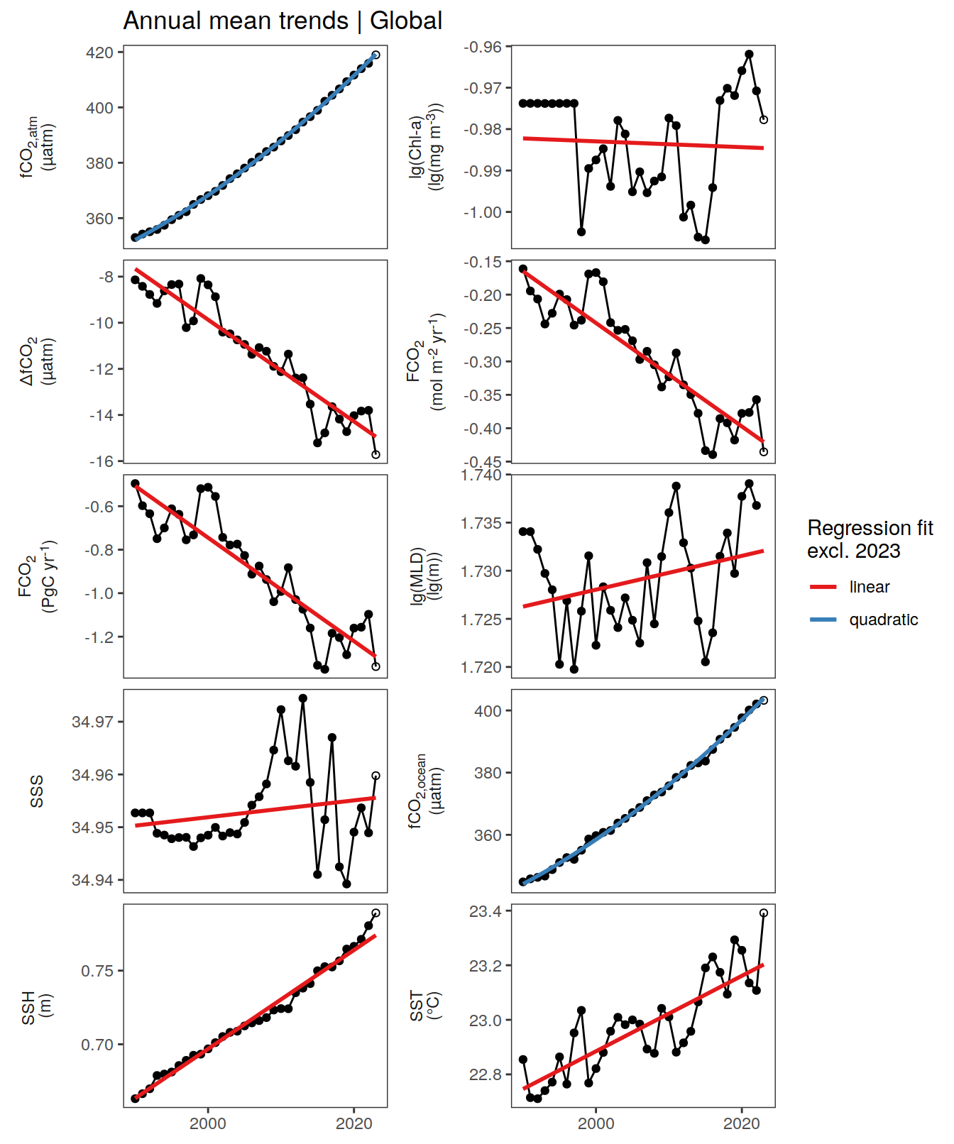
2023 anomalies
Annual mean trends
pco2_product_annual <-
  pco2_product_monthly %>%
  group_by(year, biome, name) %>%
  summarise(value = mean(value)) %>%
  ungroup()

pco2_product_annual %>%
  filter(biome %in% "Global") %>%
  ggplot(aes(year, value)) +
  geom_path() +
  geom_point(data = . %>% filter(year != 2023)) +
  geom_point(data = . %>% filter(year == 2023),
             shape = 1) +
  geom_smooth(data = . %>% filter(year != 2023,
                                  !(name %in% name_quadratic_fit)),
              method = "lm",
              fullrange = TRUE,
              aes(col = "linear"),
              se = FALSE) +
  geom_smooth(data = . %>% filter(year != 2023,
                                  name %in% name_quadratic_fit),
              method = "lm",
              fullrange = TRUE,
              formula = y ~ x + I(x^2),
              aes(col = "quadratic"),
              se = FALSE) +
  scale_color_brewer(
    palette = "Set1",
    name = paste("Regression fit\nexcl.", 2023)) +
  scale_x_continuous(breaks = seq(1980, 2020, 20)) +
  labs(title = "Annual mean trends | Global") +
  facet_wrap(name ~ .,
             scales = "free_y",
             labeller = labeller(name = x_axis_labels),
             strip.position = "left",
             ncol = 2) +
  theme(
    strip.text.y.left = element_markdown(),
    strip.placement = "outside",
    strip.background.y = element_blank(),
    axis.title = element_blank()
  )
| Version | Author | Date |
|---|---|---|
| 51df30d | jens-daniel-mueller | 2024-05-15 |
| 009791f | jens-daniel-mueller | 2024-05-14 |
| 3b5d16b | jens-daniel-mueller | 2024-05-13 |
| 77accd5 | jens-daniel-mueller | 2024-05-07 |
| e9c4ecf | jens-daniel-mueller | 2024-05-07 |
| 5d10d21 | jens-daniel-mueller | 2024-05-07 |
| dfcf790 | jens-daniel-mueller | 2024-04-11 |
| 89becff | jens-daniel-mueller | 2024-04-11 |
| 2321242 | jens-daniel-mueller | 2024-04-11 |
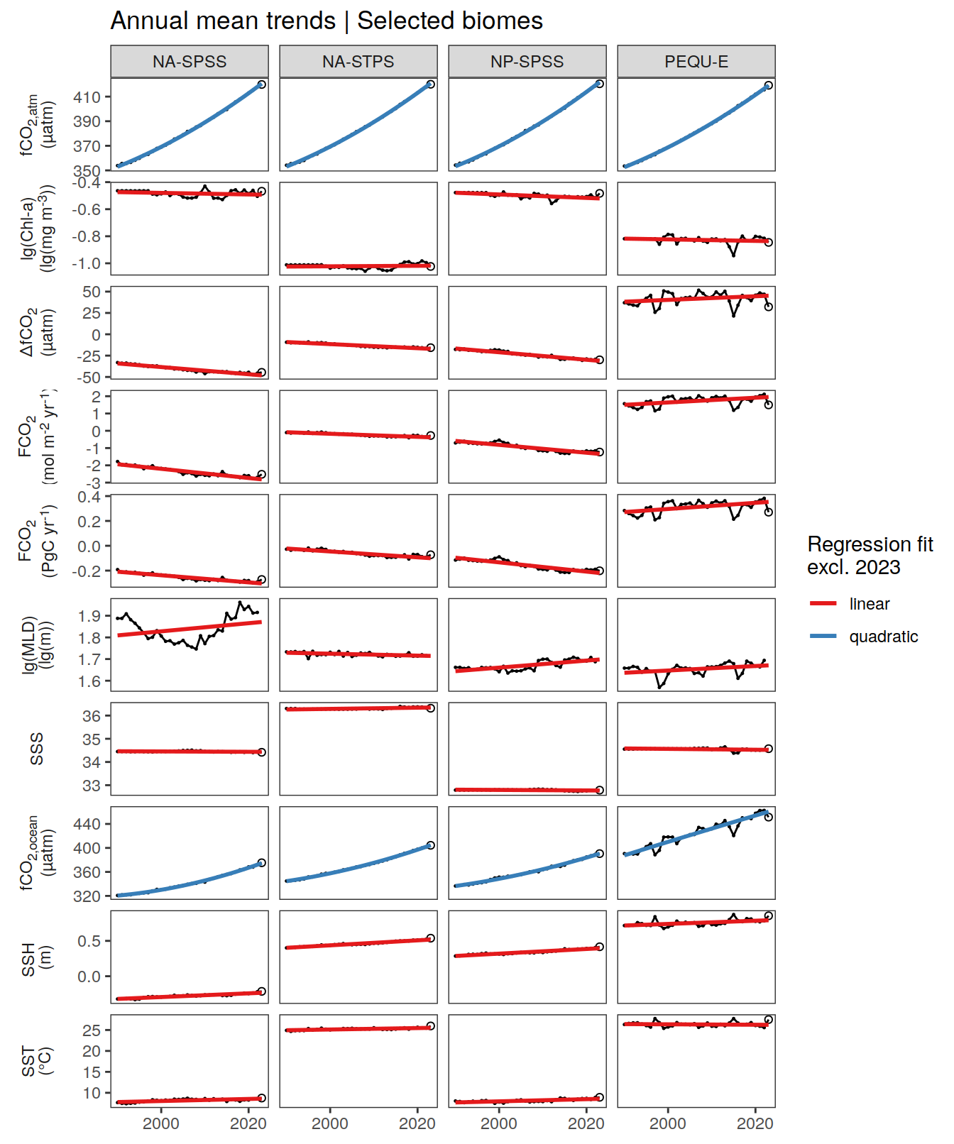
pco2_product_annual %>%
  filter(biome %in% key_biomes) %>%
  ggplot(aes(year, value)) +
  geom_path() +
  geom_point(data = . %>% filter(year != 2023),
             size = 0.2) +
  geom_point(data = . %>% filter(year == 2023),
             shape = 1) +
  geom_smooth(data = . %>% filter(year != 2023,
                                  !(name %in% name_quadratic_fit)),
              method = "lm",
              fullrange = TRUE,
              aes(col = "linear"),
              se = FALSE) +
  geom_smooth(data = . %>% filter(year != 2023,
                                  name %in% name_quadratic_fit),
              method = "lm",
              fullrange = TRUE,
              formula = y ~ x + I(x^2),
              aes(col = "quadratic"),
              se = FALSE) +
  scale_color_brewer(
    palette = "Set1",
    name = paste("Regression fit\nexcl.", 2023)) +
  scale_x_continuous(breaks = seq(1980, 2020, 20)) +
  labs(title = "Annual mean trends | Selected biomes") +
  facet_grid(name ~ biome,
             scales = "free_y",
             labeller = labeller(name = x_axis_labels),
             switch = "y") +
  theme(
    strip.text.y.left = element_markdown(),
    strip.placement = "outside",
    strip.background.y = element_blank(),
    axis.title = element_blank()
  )
| Version | Author | Date |
|---|---|---|
| 51df30d | jens-daniel-mueller | 2024-05-15 |
| 009791f | jens-daniel-mueller | 2024-05-14 |
| 3b5d16b | jens-daniel-mueller | 2024-05-13 |
| 77accd5 | jens-daniel-mueller | 2024-05-07 |
| e9c4ecf | jens-daniel-mueller | 2024-05-07 |
| 5d10d21 | jens-daniel-mueller | 2024-05-07 |
| dfcf790 | jens-daniel-mueller | 2024-04-11 |
| 89becff | jens-daniel-mueller | 2024-04-11 |
| 2321242 | jens-daniel-mueller | 2024-04-11 |
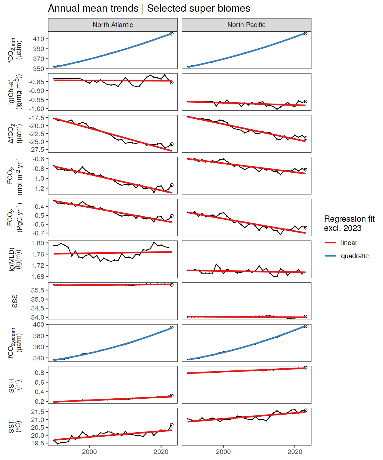
pco2_product_annual %>%
  filter(biome %in% super_biomes) %>%
  ggplot(aes(year, value)) +
  geom_path() +
  geom_point(data = . %>% filter(year != 2023),
             size = 0.2) +
  geom_point(data = . %>% filter(year == 2023),
             shape = 1) +
  geom_smooth(data = . %>% filter(year != 2023,
                                  !(name %in% name_quadratic_fit)),
              method = "lm",
              fullrange = TRUE,
              aes(col = "linear"),
              se = FALSE) +
  geom_smooth(data = . %>% filter(year != 2023,
                                  name %in% name_quadratic_fit),
              method = "lm",
              fullrange = TRUE,
              formula = y ~ x + I(x^2),
              aes(col = "quadratic"),
              se = FALSE) +
  scale_color_brewer(
    palette = "Set1",
    name = paste("Regression fit\nexcl.", 2023)) +
  scale_x_continuous(breaks = seq(1980, 2020, 20)) +
  labs(title = "Annual mean trends | Selected super biomes") +
  facet_grid(name ~ biome,
             scales = "free_y",
             labeller = labeller(name = x_axis_labels),
             switch = "y") +
  theme(
    strip.text.y.left = element_markdown(),
    strip.placement = "outside",
    strip.background.y = element_blank(),
    axis.title = element_blank()
  )
| Version | Author | Date |
|---|---|---|
| 51df30d | jens-daniel-mueller | 2024-05-15 |
| 009791f | jens-daniel-mueller | 2024-05-14 |
| 3b5d16b | jens-daniel-mueller | 2024-05-13 |
| 77accd5 | jens-daniel-mueller | 2024-05-07 |
| e9c4ecf | jens-daniel-mueller | 2024-05-07 |
| 5d10d21 | jens-daniel-mueller | 2024-05-07 |
| dfcf790 | jens-daniel-mueller | 2024-04-11 |
| 89becff | jens-daniel-mueller | 2024-04-11 |
| 2321242 | jens-daniel-mueller | 2024-04-11 |
pco2_product_annual_regression <-
pco2_product_annual %>%
anomaly_determination(biome)
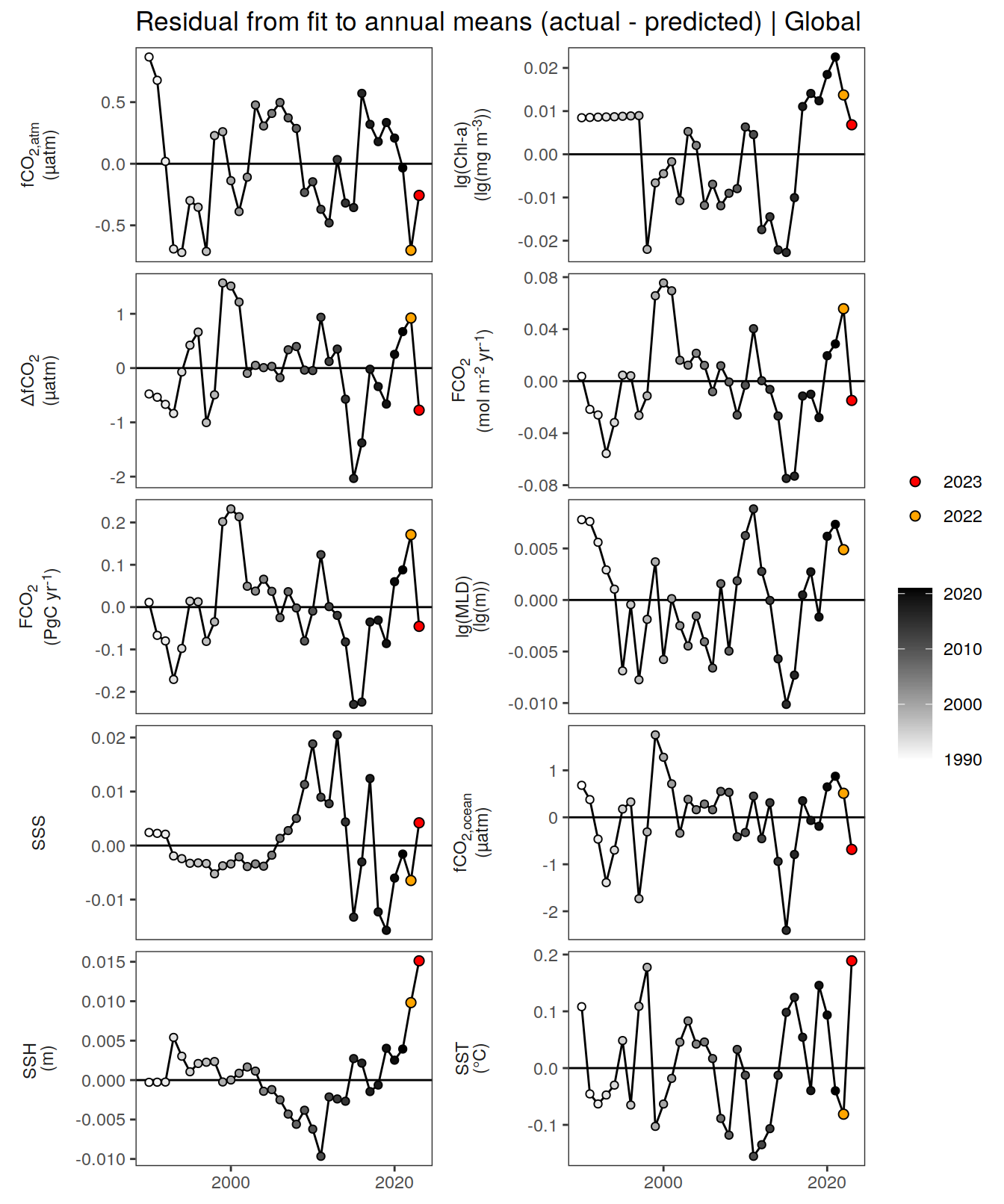
pco2_product_annual_regression %>%
filter(biome %in% "Global") %>%
ggplot(aes(year, resid)) +
geom_hline(yintercept = 0) +
geom_path() +
geom_point(data = . %>% filter(!between(year, 2023-1, 2023)),
aes(fill = year),
shape = 21) +
scale_fill_grayC() +
new_scale_fill() +
geom_point(data = . %>% filter(between(year, 2023-1, 2023)),
aes(fill = as.factor(year)),
shape = 21, size = 2) +
scale_fill_manual(values = c("orange", "red"),
guide = guide_legend(reverse = TRUE,
order = 1)) +
scale_x_continuous(breaks = seq(1980, 2020, 20)) +
labs(title = "Residual from fit to annual means (actual - predicted) | Global") +
facet_wrap(name ~ .,
scales = "free_y",
labeller = labeller(name = x_axis_labels),
strip.position = "left",
ncol = 2) +
theme(
strip.text.y.left = element_markdown(),
strip.placement = "outside",
strip.background.y = element_blank(),
axis.title = element_blank(),
legend.title = element_blank()
)
| Version | Author | Date |
|---|---|---|
| 51df30d | jens-daniel-mueller | 2024-05-15 |
| 009791f | jens-daniel-mueller | 2024-05-14 |
| 3b5d16b | jens-daniel-mueller | 2024-05-13 |
| 77accd5 | jens-daniel-mueller | 2024-05-07 |
| e9c4ecf | jens-daniel-mueller | 2024-05-07 |
| 5d10d21 | jens-daniel-mueller | 2024-05-07 |
| dfcf790 | jens-daniel-mueller | 2024-04-11 |
| 89becff | jens-daniel-mueller | 2024-04-11 |
| 2321242 | jens-daniel-mueller | 2024-04-11 |
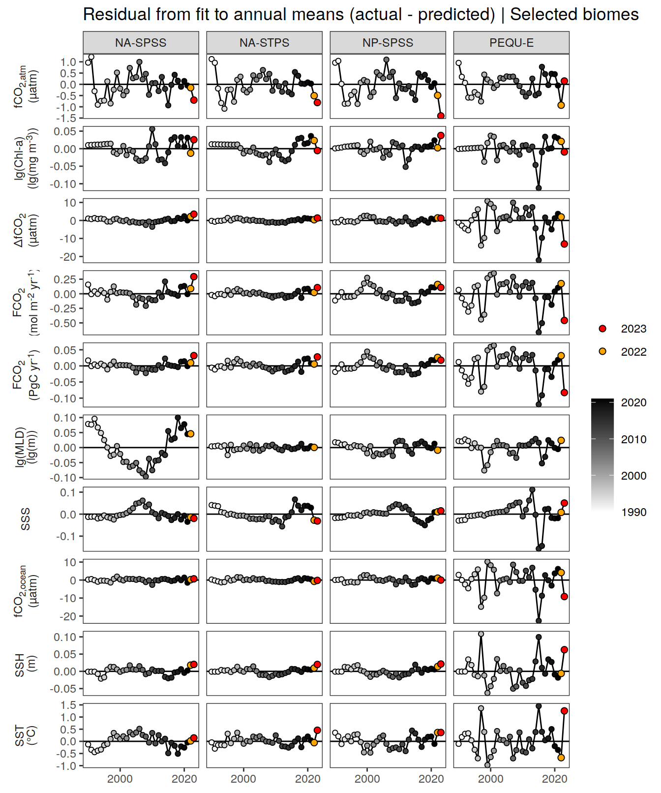
pco2_product_annual_regression %>%
  filter(biome %in% key_biomes) %>%
  ggplot(aes(year, resid)) +
  geom_hline(yintercept = 0) +
  geom_path() +
  geom_point(data = . %>% filter(!between(year, 2023-1, 2023)),
             aes(fill = year),
             shape = 21) +
  scale_fill_grayC() +
  new_scale_fill() +
  geom_point(data = . %>% filter(between(year, 2023-1, 2023)),
             aes(fill = as.factor(year)),
             shape = 21, size = 2)  +
  scale_fill_manual(values = c("orange", "red"),
                     guide = guide_legend(reverse = TRUE,
                                          order = 1)) +
  scale_x_continuous(breaks = seq(1980, 2020, 20)) +
  labs(title = "Residual from fit to annual means (actual - predicted) | Selected biomes") +
  facet_grid(name ~ biome,
             scales = "free_y",
             labeller = labeller(name = x_axis_labels),
             switch = "y") +
  theme(
    strip.text.y.left = element_markdown(),
    strip.placement = "outside",
    strip.background.y = element_blank(),
    axis.title = element_blank(),
    legend.title = element_blank()
  )
| Version | Author | Date |
|---|---|---|
| 51df30d | jens-daniel-mueller | 2024-05-15 |
| 009791f | jens-daniel-mueller | 2024-05-14 |
| 3b5d16b | jens-daniel-mueller | 2024-05-13 |
| 77accd5 | jens-daniel-mueller | 2024-05-07 |
| e9c4ecf | jens-daniel-mueller | 2024-05-07 |
| 5d10d21 | jens-daniel-mueller | 2024-05-07 |
| dfcf790 | jens-daniel-mueller | 2024-04-11 |
| 89becff | jens-daniel-mueller | 2024-04-11 |
| 2321242 | jens-daniel-mueller | 2024-04-11 |
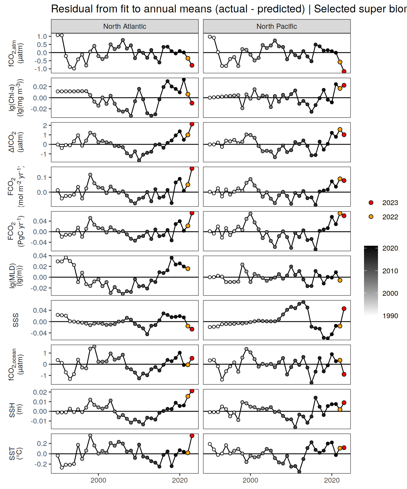
pco2_product_annual_regression %>%
  filter(biome %in% super_biomes) %>%
  ggplot(aes(year, resid)) +
  geom_hline(yintercept = 0) +
  geom_path() +
  geom_point(data = . %>% filter(!between(year, 2023-1, 2023)),
             aes(fill = year),
             shape = 21) +
  scale_fill_grayC() +
  new_scale_fill() +
  geom_point(data = . %>% filter(between(year, 2023-1, 2023)),
             aes(fill = as.factor(year)),
             shape = 21, size = 2)  +
  scale_fill_manual(values = c("orange", "red"),
                     guide = guide_legend(reverse = TRUE,
                                          order = 1)) +
  scale_x_continuous(breaks = seq(1980, 2020, 20)) +
  labs(title = "Residual from fit to annual means (actual - predicted) | Selected super biomes") +
  facet_grid(name ~ biome,
             scales = "free_y",
             labeller = labeller(name = x_axis_labels),
             switch = "y") +
  theme(
    strip.text.y.left = element_markdown(),
    strip.placement = "outside",
    strip.background.y = element_blank(),
    axis.title = element_blank(),
    legend.title = element_blank()
  )
| Version | Author | Date |
|---|---|---|
| 51df30d | jens-daniel-mueller | 2024-05-15 |
| 009791f | jens-daniel-mueller | 2024-05-14 |
| 3b5d16b | jens-daniel-mueller | 2024-05-13 |
| 77accd5 | jens-daniel-mueller | 2024-05-07 |
| e9c4ecf | jens-daniel-mueller | 2024-05-07 |
| 5d10d21 | jens-daniel-mueller | 2024-05-07 |
| dfcf790 | jens-daniel-mueller | 2024-04-11 |
| 89becff | jens-daniel-mueller | 2024-04-11 |
| 2321242 | jens-daniel-mueller | 2024-04-11 |
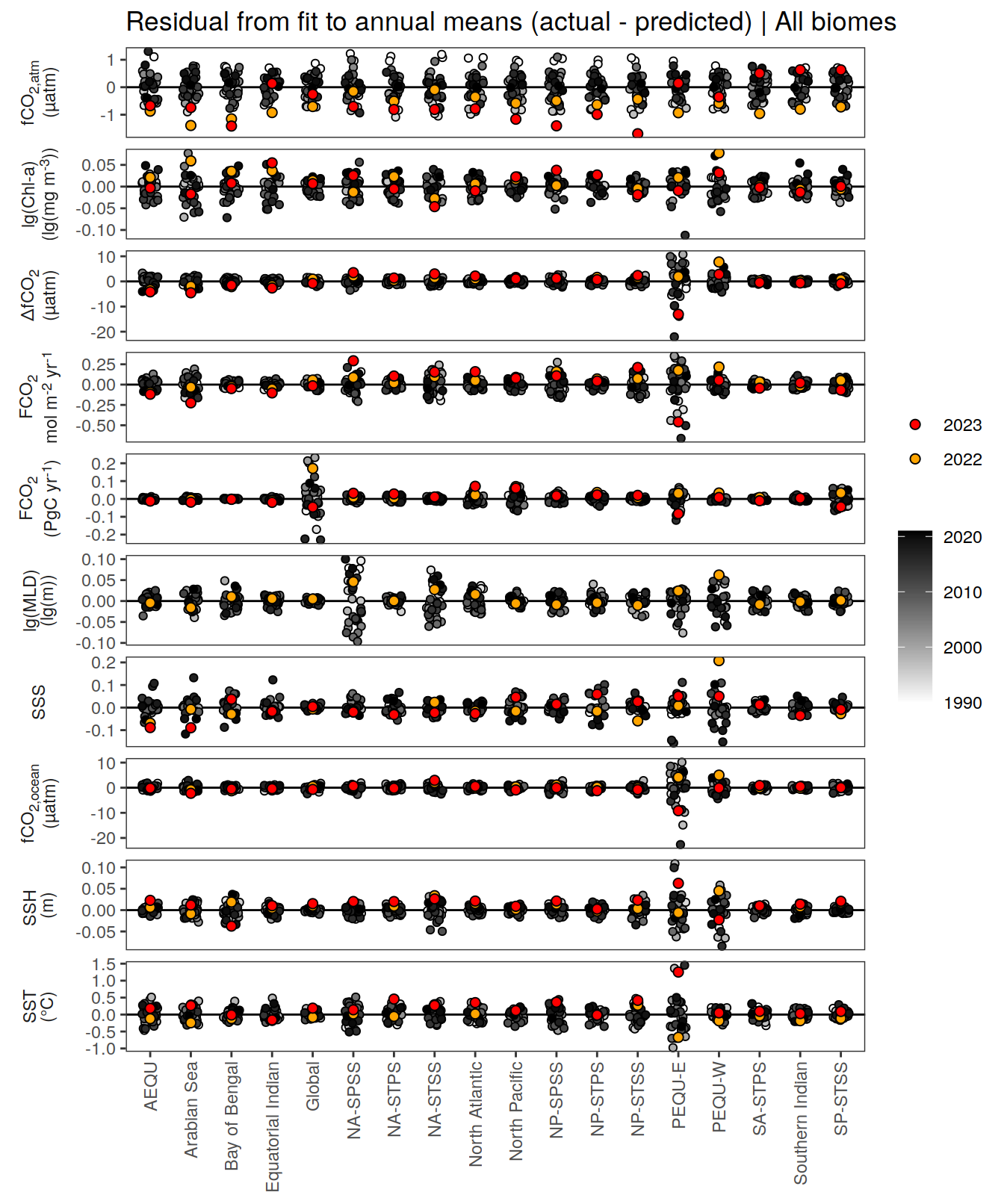
pco2_product_annual_regression %>%
  filter(biome != "global") %>%
  ggplot(aes(biome, resid)) +
  geom_hline(yintercept = 0) +
  geom_jitter(data = . %>% filter(!between(year, 2023-1, 2023)),
             aes(fill = year),
             shape = 21, width = 0.2) +
  scale_fill_grayC() +
  new_scale_fill() +
  geom_point(data = . %>% filter(between(year, 2023-1, 2023)),
             aes(fill = as.factor(year)),
             shape = 21, size = 2)  +
  scale_fill_manual(values = c("orange", "red"),
                     guide = guide_legend(reverse = TRUE,
                                          order = 1)) +
  labs(title = "Residual from fit to annual means (actual - predicted) | All biomes") +
  facet_grid(name ~ .,
             scales = "free_y",
             labeller = labeller(name = x_axis_labels),
             switch = "y") +
  theme(
    strip.text.y.left = element_markdown(),
    strip.placement = "outside",
    strip.background.y = element_blank(),
    axis.title = element_blank(),
    legend.title = element_blank(),
        axis.text.x = element_text(angle = 90, vjust = 0.5, hjust=1)
  )
| Version | Author | Date |
|---|---|---|
| 51df30d | jens-daniel-mueller | 2024-05-15 |
| 009791f | jens-daniel-mueller | 2024-05-14 |
| 3b5d16b | jens-daniel-mueller | 2024-05-13 |
| 77accd5 | jens-daniel-mueller | 2024-05-07 |
| e9c4ecf | jens-daniel-mueller | 2024-05-07 |
| 5d10d21 | jens-daniel-mueller | 2024-05-07 |
| dfcf790 | jens-daniel-mueller | 2024-04-11 |
| 89becff | jens-daniel-mueller | 2024-04-11 |
| 2321242 | jens-daniel-mueller | 2024-04-11 |
pco2_product_annual_regression %>%
  write_csv(paste0("../data/","CMEMS","_","2023","_biome_annual_regression.csv"))
pco2_product_annual_detrended <-
full_join(pco2_product_monthly,
pco2_product_annual_regression %>% select(-c(value, resid))) %>%
mutate(resid = value - fit)
pco2_product_annual_detrended %>%
filter(biome %in% "Global") %>%
ggplot(aes(month, resid, group = as.factor(year))) +
geom_path(data = . %>% filter(!between(year, 2023-1, 2023)),
aes(col = year)) +
scale_color_grayC() +
new_scale_color() +
geom_path(data = . %>% filter(between(year, 2023-1, 2023)),
aes(col = as.factor(year)),
linewidth = 1) +
scale_color_manual(values = c("orange", "red"),
guide = guide_legend(reverse = TRUE,
order = 1)) +
scale_x_continuous(breaks = seq(1, 12, 3), expand = c(0, 0)) +
labs(title = "Anomalies from predicted annual mean | Global") +
facet_wrap(name ~ .,
scales = "free_y",
labeller = labeller(name = x_axis_labels),
strip.position = "left",
ncol = 2) +
theme(
strip.text.y.left = element_markdown(),
strip.placement = "outside",
strip.background.y = element_blank(),
axis.title.y = element_blank(),
legend.title = element_blank()
)
| Version | Author | Date |
|---|---|---|
| 51df30d | jens-daniel-mueller | 2024-05-15 |
| 009791f | jens-daniel-mueller | 2024-05-14 |
| 3b5d16b | jens-daniel-mueller | 2024-05-13 |
| 77accd5 | jens-daniel-mueller | 2024-05-07 |
| e9c4ecf | jens-daniel-mueller | 2024-05-07 |
| 5d10d21 | jens-daniel-mueller | 2024-05-07 |
| dfcf790 | jens-daniel-mueller | 2024-04-11 |
| 89becff | jens-daniel-mueller | 2024-04-11 |
| 2321242 | jens-daniel-mueller | 2024-04-11 |
pco2_product_annual_detrended %>%
  filter(biome %in% key_biomes) %>%
  ggplot(aes(month, resid, group = as.factor(year))) +
  geom_path(data = . %>% filter(!between(year, 2023-1, 2023)),
            aes(col = year)) +
  scale_color_grayC() +
  new_scale_color() +
  geom_path(data = . %>% filter(between(year, 2023-1, 2023)),
            aes(col = as.factor(year)),
            linewidth = 1) +
  scale_color_manual(values = c("orange", "red"),
                     guide = guide_legend(reverse = TRUE,
                                          order = 1)) +
  scale_x_continuous(breaks = seq(1, 12, 3), expand = c(0, 0)) +
  labs(title = "Anomalies from predicted annual mean | Selected biomes") +
  facet_grid(name ~ biome,
             scales = "free_y",
             labeller = labeller(name = x_axis_labels),
             switch = "y") +
  theme(
    strip.text.y.left = element_markdown(),
    strip.placement = "outside",
    strip.background.y = element_blank(),
    axis.title.y = element_blank(),
    legend.title = element_blank(),
        axis.text.x = element_text(angle = 90, vjust = 0.5, hjust=1)
  )
| Version | Author | Date |
|---|---|---|
| 51df30d | jens-daniel-mueller | 2024-05-15 |
| 009791f | jens-daniel-mueller | 2024-05-14 |
| 3b5d16b | jens-daniel-mueller | 2024-05-13 |
| 77accd5 | jens-daniel-mueller | 2024-05-07 |
| e9c4ecf | jens-daniel-mueller | 2024-05-07 |
| 5d10d21 | jens-daniel-mueller | 2024-05-07 |
| dfcf790 | jens-daniel-mueller | 2024-04-11 |
| 89becff | jens-daniel-mueller | 2024-04-11 |
| 2321242 | jens-daniel-mueller | 2024-04-11 |
pco2_product_annual_detrended %>%
  filter(biome %in% super_biomes) %>%
  ggplot(aes(month, resid, group = as.factor(year))) +
  geom_path(data = . %>% filter(!between(year, 2023-1, 2023)),
            aes(col = year)) +
  scale_color_grayC() +
  new_scale_color() +
  geom_path(data = . %>% filter(between(year, 2023-1, 2023)),
            aes(col = as.factor(year)),
            linewidth = 1) +
  scale_color_manual(values = c("orange", "red"),
                     guide = guide_legend(reverse = TRUE,
                                          order = 1)) +
  scale_x_continuous(breaks = seq(1, 12, 3), expand = c(0, 0)) +
  labs(title = "Anomalies from predicted annual mean | Selected super biomes") +
  facet_grid(name ~ biome,
             scales = "free_y",
             labeller = labeller(name = x_axis_labels),
             switch = "y") +
  theme(
    strip.text.y.left = element_markdown(),
    strip.placement = "outside",
    strip.background.y = element_blank(),
    axis.title.y = element_blank(),
    legend.title = element_blank(),
        axis.text.x = element_text(angle = 90, vjust = 0.5, hjust=1)
  )
| Version | Author | Date |
|---|---|---|
| 51df30d | jens-daniel-mueller | 2024-05-15 |
| 009791f | jens-daniel-mueller | 2024-05-14 |
| 3b5d16b | jens-daniel-mueller | 2024-05-13 |
| 77accd5 | jens-daniel-mueller | 2024-05-07 |
| e9c4ecf | jens-daniel-mueller | 2024-05-07 |
| 5d10d21 | jens-daniel-mueller | 2024-05-07 |
| dfcf790 | jens-daniel-mueller | 2024-04-11 |
| 89becff | jens-daniel-mueller | 2024-04-11 |
| 2321242 | jens-daniel-mueller | 2024-04-11 |
pco2_product_annual_detrended %>%
  filter(biome %in% key_biomes) %>%
  group_split(biome) %>%
  # head(1) %>%
  map(
    ~ ggplot(data = .x,
             aes(month, resid, group = as.factor(year))) +
      geom_path(data = . %>% filter(!between(year, 2023-1, 2023)),
                aes(col = year)) +
      scale_color_grayC() +
      new_scale_color() +
      geom_path(
        data = . %>% filter(between(year, 2023-1, 2023)),
        aes(col = as.factor(year)),
        linewidth = 1
      ) +
      scale_color_manual(
        values = c("orange", "red"),
        guide = guide_legend(reverse = TRUE,
                             order = 1)
      ) +
      scale_x_continuous(breaks = seq(1, 12, 3), expand = c(0, 0)) +
      labs(title = paste("Anomalies from predicted annual mean |", .x$biome)) +
      facet_wrap(
        name ~ .,
        scales = "free_y",
        labeller = labeller(name = x_axis_labels),
        strip.position = "left",
        ncol = 2
      ) +
      theme(
        strip.text.y.left = element_markdown(),
        strip.placement = "outside",
        strip.background.y = element_blank(),
        axis.title = element_blank(),
        legend.title = element_blank()
      )
  )
[[1]]
| Version | Author | Date |
|---|---|---|
| 51df30d | jens-daniel-mueller | 2024-05-15 |
| 3b5d16b | jens-daniel-mueller | 2024-05-13 |
| 77accd5 | jens-daniel-mueller | 2024-05-07 |
| e9c4ecf | jens-daniel-mueller | 2024-05-07 |
| 5d10d21 | jens-daniel-mueller | 2024-05-07 |
| dfcf790 | jens-daniel-mueller | 2024-04-11 |
| 89becff | jens-daniel-mueller | 2024-04-11 |
| 2321242 | jens-daniel-mueller | 2024-04-11 |
[[2]]
| Version | Author | Date |
|---|---|---|
| 51df30d | jens-daniel-mueller | 2024-05-15 |
| 3b5d16b | jens-daniel-mueller | 2024-05-13 |
| 77accd5 | jens-daniel-mueller | 2024-05-07 |
| e9c4ecf | jens-daniel-mueller | 2024-05-07 |
| 5d10d21 | jens-daniel-mueller | 2024-05-07 |
| dfcf790 | jens-daniel-mueller | 2024-04-11 |
| 89becff | jens-daniel-mueller | 2024-04-11 |
| 2321242 | jens-daniel-mueller | 2024-04-11 |
[[3]]
| Version | Author | Date |
|---|---|---|
| 51df30d | jens-daniel-mueller | 2024-05-15 |
| 3b5d16b | jens-daniel-mueller | 2024-05-13 |
| 77accd5 | jens-daniel-mueller | 2024-05-07 |
| e9c4ecf | jens-daniel-mueller | 2024-05-07 |
| 5d10d21 | jens-daniel-mueller | 2024-05-07 |
| dfcf790 | jens-daniel-mueller | 2024-04-11 |
| 89becff | jens-daniel-mueller | 2024-04-11 |
| 2321242 | jens-daniel-mueller | 2024-04-11 |
[[4]]
| Version | Author | Date |
|---|---|---|
| 51df30d | jens-daniel-mueller | 2024-05-15 |
| 3b5d16b | jens-daniel-mueller | 2024-05-13 |
| 77accd5 | jens-daniel-mueller | 2024-05-07 |
| e9c4ecf | jens-daniel-mueller | 2024-05-07 |
| 5d10d21 | jens-daniel-mueller | 2024-05-07 |
| dfcf790 | jens-daniel-mueller | 2024-04-11 |
| 89becff | jens-daniel-mueller | 2024-04-11 |
| 2321242 | jens-daniel-mueller | 2024-04-11 |
pco2_product_annual_detrended %>%
  filter(biome %in% super_biomes) %>%
  group_split(biome) %>%
  # head(1) %>%
  map(
    ~ ggplot(data = .x,
             aes(month, resid, group = as.factor(year))) +
      geom_path(data = . %>% filter(!between(year, 2023-1, 2023)),
                aes(col = year)) +
      scale_color_grayC() +
      new_scale_color() +
      geom_path(
        data = . %>% filter(between(year, 2023-1, 2023)),
        aes(col = as.factor(year)),
        linewidth = 1
      ) +
      scale_color_manual(
        values = c("orange", "red"),
        guide = guide_legend(reverse = TRUE,
                             order = 1)
      ) +
      scale_x_continuous(breaks = seq(1, 12, 3), expand = c(0, 0)) +
      labs(title = paste("Anomalies from predicted annual mean |", .x$biome)) +
      facet_wrap(
        name ~ .,
        scales = "free_y",
        labeller = labeller(name = x_axis_labels),
        strip.position = "left",
        ncol = 2
      ) +
      theme(
        strip.text.y.left = element_markdown(),
        strip.placement = "outside",
        strip.background.y = element_blank(),
        axis.title = element_blank(),
        legend.title = element_blank()
      )
  )
[[1]]
| Version | Author | Date |
|---|---|---|
| 51df30d | jens-daniel-mueller | 2024-05-15 |
| 3b5d16b | jens-daniel-mueller | 2024-05-13 |
| 77accd5 | jens-daniel-mueller | 2024-05-07 |
| e9c4ecf | jens-daniel-mueller | 2024-05-07 |
| 5d10d21 | jens-daniel-mueller | 2024-05-07 |
| dfcf790 | jens-daniel-mueller | 2024-04-11 |
| 89becff | jens-daniel-mueller | 2024-04-11 |
| 2321242 | jens-daniel-mueller | 2024-04-11 |
[[2]]
| Version | Author | Date |
|---|---|---|
| 51df30d | jens-daniel-mueller | 2024-05-15 |
| 3b5d16b | jens-daniel-mueller | 2024-05-13 |
| 77accd5 | jens-daniel-mueller | 2024-05-07 |
| e9c4ecf | jens-daniel-mueller | 2024-05-07 |
| 5d10d21 | jens-daniel-mueller | 2024-05-07 |
| dfcf790 | jens-daniel-mueller | 2024-04-11 |
| 89becff | jens-daniel-mueller | 2024-04-11 |
| 2321242 | jens-daniel-mueller | 2024-04-11 |
pco2_product_annual_detrended %>%
  write_csv(paste0("../data/","CMEMS","_","2023","_biome_annual_detrended.csv"))
Monthly mean trends
pco2_product_monthly %>%
  filter(biome %in% "Global") %>%
  mutate(month = as.factor(month)) %>%
  ggplot(aes(year, value, col = month)) +
  # geom_point() +
  geom_smooth(data = . %>% filter(year != 2023,
                                  !(name %in% name_quadratic_fit)),
              method = "lm",
              se = FALSE,
              fullrange = TRUE) +
  geom_smooth(
    data = . %>% filter(year != 2023,
                        name %in% name_quadratic_fit),
    method = "lm",
    fullrange = TRUE,
    formula = y ~ x + I(x ^ 2),
    se = FALSE
  ) +
  scale_color_scico_d(palette = "romaO",
    name = paste("Regression fit\nexcl.", 2023)) +
  scale_x_continuous(breaks = seq(1980, 2020, 20)) +
  labs(title = "Monthly mean trends | Global") +
  facet_wrap(name ~ .,
             scales = "free_y",
             labeller = labeller(name = x_axis_labels),
             strip.position = "left",
             ncol = 2) +
  theme(
    strip.text.y.left = element_markdown(),
    strip.placement = "outside",
    strip.background.y = element_blank(),
    axis.title = element_blank()
  )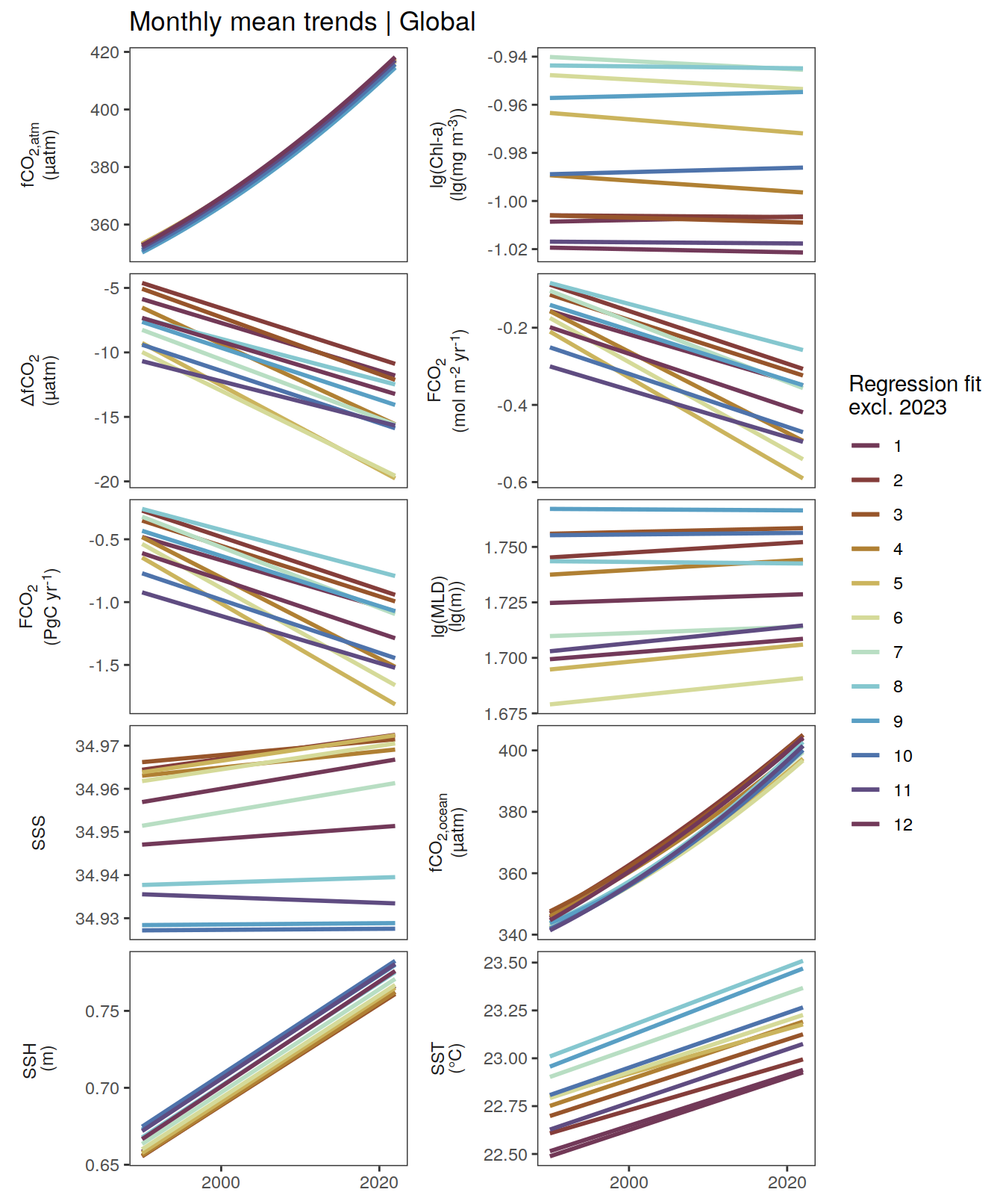
| Version | Author | Date |
|---|---|---|
| 51df30d | jens-daniel-mueller | 2024-05-15 |
| 009791f | jens-daniel-mueller | 2024-05-14 |
| 3b5d16b | jens-daniel-mueller | 2024-05-13 |
| e9c4ecf | jens-daniel-mueller | 2024-05-07 |
| 5d10d21 | jens-daniel-mueller | 2024-05-07 |
| dfcf790 | jens-daniel-mueller | 2024-04-11 |
| 89becff | jens-daniel-mueller | 2024-04-11 |
| 2321242 | jens-daniel-mueller | 2024-04-11 |
pco2_product_monthly %>%
  filter(biome %in% key_biomes) %>%
  mutate(month = as.factor(month)) %>%
  ggplot(aes(year, value, col = month)) +
  # geom_point() +
  geom_smooth(data = . %>% filter(year != 2023,
                                  !(name %in% name_quadratic_fit)),
              method = "lm",
              fullrange = TRUE,
              se = FALSE) +
  geom_smooth(
    data = . %>% filter(year != 2023,
                        name %in% name_quadratic_fit),
    method = "lm",
    fullrange = TRUE,
    formula = y ~ x + I(x ^ 2),
    se = FALSE
  ) +
  scale_color_scico_d(palette = "romaO",
    name = paste("Regression fit\nexcl.", 2023)) +
  scale_x_continuous(breaks = seq(1980, 2020, 20)) +
  labs(title = "Monthly mean trends | Selected biomes") +
  facet_grid(name ~ biome,
             scales = "free_y",
             labeller = labeller(name = x_axis_labels),
             switch = "y") +
  theme(
    strip.text.y.left = element_markdown(),
    strip.placement = "outside",
    strip.background.y = element_blank(),
    axis.title = element_blank()
  )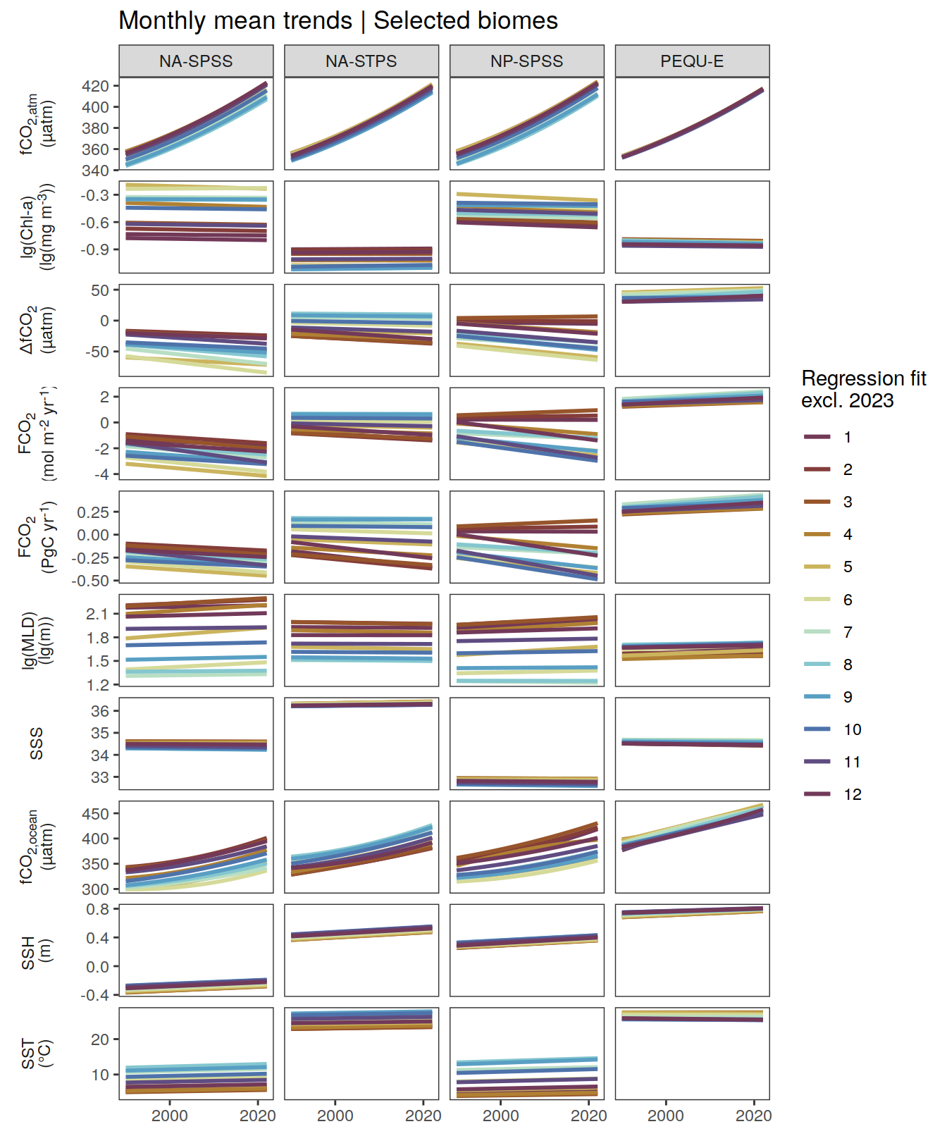
| Version | Author | Date |
|---|---|---|
| 51df30d | jens-daniel-mueller | 2024-05-15 |
| 009791f | jens-daniel-mueller | 2024-05-14 |
| 3b5d16b | jens-daniel-mueller | 2024-05-13 |
| e9c4ecf | jens-daniel-mueller | 2024-05-07 |
| 5d10d21 | jens-daniel-mueller | 2024-05-07 |
| dfcf790 | jens-daniel-mueller | 2024-04-11 |
| 89becff | jens-daniel-mueller | 2024-04-11 |
| 2321242 | jens-daniel-mueller | 2024-04-11 |
pco2_product_monthly_regression <-
  pco2_product_monthly %>%
  anomaly_determination(biome, month)


pco2_product_monthly_regression %>%
  filter(biome %in% "Global") %>%
  group_split(month) %>%
  head(1) %>%
  map(
    ~ ggplot(data = .x,
             aes(year, resid)) +
      geom_hline(yintercept = 0) +
      geom_path() +
      geom_point(
        data = . %>% filter(!between(year, 2023-1, 2023)),
        aes(fill = year),
        shape = 21
      ) +
      scale_fill_grayC() +
      new_scale_fill() +
      geom_point(
        data = . %>% filter(between(year, 2023-1, 2023)),
        aes(fill = as.factor(year)),
        shape = 21,
        size = 2
      )  +
      scale_fill_manual(
        values = c("orange", "red"),
        guide = guide_legend(reverse = TRUE,
                             order = 1)
      ) +
      scale_x_continuous(breaks = seq(1980, 2020, 20)) +
      labs(title = "Residual from fit to monthly means (actual - predicted) | Global",
           subtitle = paste("Month:", .x$month)) +
      facet_wrap(
        name ~ .,
        scales = "free_y",
        labeller = labeller(name = x_axis_labels),
        strip.position = "left",
        ncol = 2
      ) +
      theme(
        strip.text.y.left = element_markdown(),
        strip.placement = "outside",
        strip.background.y = element_blank(),
        axis.title = element_blank(),
        legend.title = element_blank()
      )
  )
[[1]]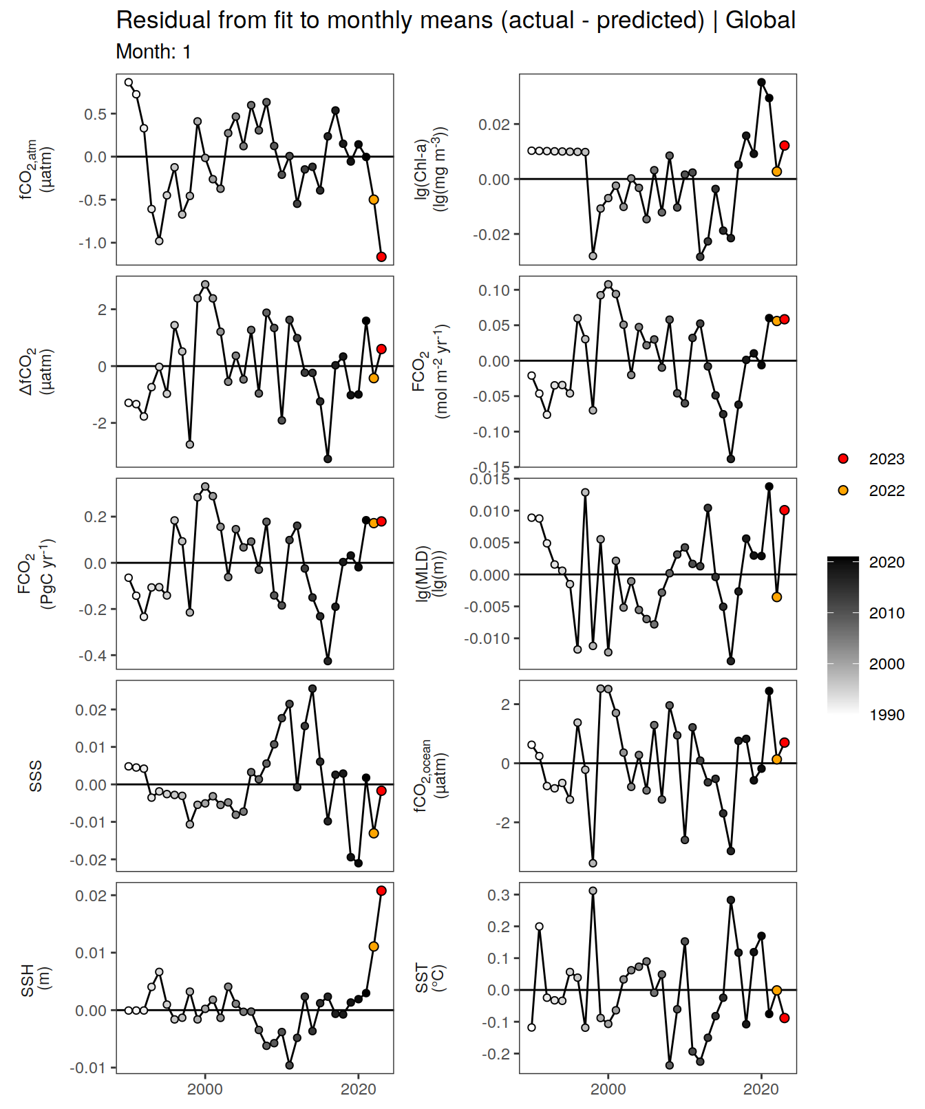
| Version | Author | Date |
|---|---|---|
| 51df30d | jens-daniel-mueller | 2024-05-15 |
| 009791f | jens-daniel-mueller | 2024-05-14 |
| 3b5d16b | jens-daniel-mueller | 2024-05-13 |
| e9c4ecf | jens-daniel-mueller | 2024-05-07 |
| 5d10d21 | jens-daniel-mueller | 2024-05-07 |
| dfcf790 | jens-daniel-mueller | 2024-04-11 |
| 89becff | jens-daniel-mueller | 2024-04-11 |
| 2321242 | jens-daniel-mueller | 2024-04-11 |
pco2_product_monthly_regression %>%
  filter(biome %in% key_biomes) %>%
  group_split(month) %>%
  head(1) %>%
  map(
    ~ ggplot(data = .x,
             aes(year, resid)) +
      geom_hline(yintercept = 0) +
      geom_path() +
      geom_point(
        data = . %>% filter(!between(year, 2023-1, 2023)),
        aes(fill = year),
        shape = 21
      ) +
      scale_fill_grayC() +
      new_scale_fill() +
      geom_point(
        data = . %>% filter(between(year, 2023-1, 2023)),
        aes(fill = as.factor(year)),
        shape = 21,
        size = 2
      )  +
      scale_fill_manual(
        values = c("orange", "red"),
        guide = guide_legend(reverse = TRUE,
                             order = 1)
      ) +
      scale_x_continuous(breaks = seq(1980, 2020, 20)) +
      labs(title = "Residual from fit to monthly means (actual - predicted) | Selected biomes",
           subtitle = paste("Month:", .x$month)) +
      facet_grid(
        name ~ biome,
        scales = "free_y",
        labeller = labeller(name = x_axis_labels),
        switch = "y"
      ) +
      theme(
        strip.text.y.left = element_markdown(),
        strip.placement = "outside",
        strip.background.y = element_blank(),
        axis.title = element_blank(),
        legend.title = element_blank()
      )
  )
[[1]]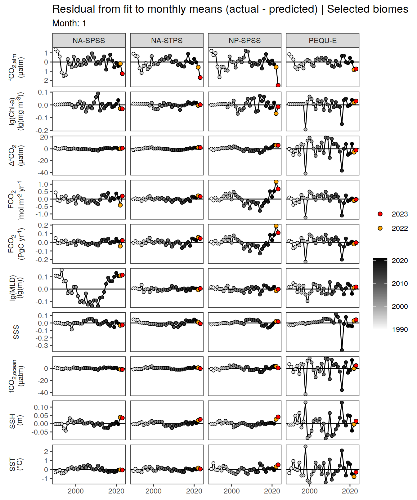
| Version | Author | Date |
|---|---|---|
| 51df30d | jens-daniel-mueller | 2024-05-15 |
| 009791f | jens-daniel-mueller | 2024-05-14 |
| 3b5d16b | jens-daniel-mueller | 2024-05-13 |
| e9c4ecf | jens-daniel-mueller | 2024-05-07 |
| 5d10d21 | jens-daniel-mueller | 2024-05-07 |
| dfcf790 | jens-daniel-mueller | 2024-04-11 |
| 89becff | jens-daniel-mueller | 2024-04-11 |
| 2321242 | jens-daniel-mueller | 2024-04-11 |
pco2_product_monthly_regression %>%
  write_csv(paste0("../data/","CMEMS","_","2023","_biome_monthly_regression.csv"))
Global
pco2_product_monthly_detrended <-
  full_join(pco2_product_monthly,
            pco2_product_monthly_regression %>% select(-c(value, resid, time))) %>%
  mutate(resid = value - fit)

pco2_product_monthly_detrended %>%
  filter(biome %in% "Global") %>%
  ggplot(aes(month, resid, group = as.factor(year))) +
  geom_path(data = . %>% filter(!between(year, 2023-1, 2023)),
            aes(col = year)) +
  scale_color_grayC() +
  new_scale_color() +
  geom_path(data = . %>% filter(between(year, 2023-1, 2023)),
            aes(col = as.factor(year)),
            linewidth = 1) +
  scale_color_manual(values = c("orange", "red"),
                     guide = guide_legend(reverse = TRUE,
                                          order = 1)) +
  scale_x_continuous(breaks = seq(1, 12, 3), expand = c(0, 0)) +
  labs(title = "Anomalies from predicted monthly mean | Global") +
  facet_wrap(
    name ~ .,
    scales = "free_y",
    labeller = labeller(name = x_axis_labels),
    strip.position = "left",
    ncol = 2
  ) +
  theme(
    strip.text.y.left = element_markdown(),
    strip.placement = "outside",
    strip.background.y = element_blank(),
    axis.title.y = element_blank(),
    legend.title = element_blank()
  )
| Version | Author | Date |
|---|---|---|
| 51df30d | jens-daniel-mueller | 2024-05-15 |
| 009791f | jens-daniel-mueller | 2024-05-14 |
| 3b5d16b | jens-daniel-mueller | 2024-05-13 |
| 77accd5 | jens-daniel-mueller | 2024-05-07 |
| e9c4ecf | jens-daniel-mueller | 2024-05-07 |
| 5d10d21 | jens-daniel-mueller | 2024-05-07 |
| dfcf790 | jens-daniel-mueller | 2024-04-11 |
| 89becff | jens-daniel-mueller | 2024-04-11 |
| 2321242 | jens-daniel-mueller | 2024-04-11 |
pco2_product_monthly_detrended %>%
  filter(biome %in% key_biomes) %>%
  ggplot(aes(month, resid, group = as.factor(year))) +
  geom_path(data = . %>% filter(!between(year, 2023-1, 2023)),
            aes(col = year)) +
  scale_color_grayC() +
  new_scale_color() +
  geom_path(data = . %>% filter(between(year, 2023-1, 2023)),
            aes(col = as.factor(year)),
            linewidth = 1) +
  scale_color_manual(values = c("orange", "red"),
                     guide = guide_legend(reverse = TRUE,
                                          order = 1)) +
  scale_x_continuous(breaks = seq(1, 12, 3), expand = c(0, 0)) +
  labs(title = "Anomalies from predicted monthly mean | Selected biomes") +
  facet_grid(
    name ~ biome,
    scales = "free_y",
    labeller = labeller(name = x_axis_labels),
    switch = "y"
  ) +
  theme(
    strip.text.y.left = element_markdown(),
    strip.placement = "outside",
    strip.background.y = element_blank(),
    axis.title.y = element_blank(),
    legend.title = element_blank()
  )
| Version | Author | Date |
|---|---|---|
| 51df30d | jens-daniel-mueller | 2024-05-15 |
| 009791f | jens-daniel-mueller | 2024-05-14 |
| 3b5d16b | jens-daniel-mueller | 2024-05-13 |
| 77accd5 | jens-daniel-mueller | 2024-05-07 |
| e9c4ecf | jens-daniel-mueller | 2024-05-07 |
| 5d10d21 | jens-daniel-mueller | 2024-05-07 |
| dfcf790 | jens-daniel-mueller | 2024-04-11 |
| 89becff | jens-daniel-mueller | 2024-04-11 |
| 2321242 | jens-daniel-mueller | 2024-04-11 |
pco2_product_monthly_detrended %>%
  filter(biome %in% super_biomes) %>%
  ggplot(aes(month, resid, group = as.factor(year))) +
  geom_path(data = . %>% filter(!between(year, 2023-1, 2023)),
            aes(col = year)) +
  scale_color_grayC() +
  new_scale_color() +
  geom_path(data = . %>% filter(between(year, 2023-1, 2023)),
            aes(col = as.factor(year)),
            linewidth = 1) +
  scale_color_manual(values = c("orange", "red"),
                     guide = guide_legend(reverse = TRUE,
                                          order = 1)) +
  scale_x_continuous(breaks = seq(1, 12, 3), expand = c(0, 0)) +
  labs(title = "Anomalies from predicted monthly mean | Selected super biomes") +
  facet_grid(
    name ~ biome,
    scales = "free_y",
    labeller = labeller(name = x_axis_labels),
    switch = "y"
  ) +
  theme(
    strip.text.y.left = element_markdown(),
    strip.placement = "outside",
    strip.background.y = element_blank(),
    axis.title.y = element_blank(),
    legend.title = element_blank()
  )
| Version | Author | Date |
|---|---|---|
| 51df30d | jens-daniel-mueller | 2024-05-15 |
| 009791f | jens-daniel-mueller | 2024-05-14 |
| 3b5d16b | jens-daniel-mueller | 2024-05-13 |
| 77accd5 | jens-daniel-mueller | 2024-05-07 |
| e9c4ecf | jens-daniel-mueller | 2024-05-07 |
| 5d10d21 | jens-daniel-mueller | 2024-05-07 |
| dfcf790 | jens-daniel-mueller | 2024-04-11 |
| 89becff | jens-daniel-mueller | 2024-04-11 |
| 2321242 | jens-daniel-mueller | 2024-04-11 |
Selected biomes
pco2_product_monthly_detrended %>%
  filter(biome %in% key_biomes) %>%
  ggplot(aes(month, resid, group = as.factor(year))) +
  geom_path(data = . %>% filter(!between(year, 2023-1, 2023)),
            aes(col = year)) +
  scale_color_grayC() +
  new_scale_color() +
  geom_path(data = . %>% filter(between(year, 2023-1, 2023)),
            aes(col = as.factor(year)),
            linewidth = 1) +
  scale_color_manual(values = c("orange", "red"),
                     guide = guide_legend(reverse = TRUE,
                                          order = 1)) +
  scale_x_continuous(breaks = seq(1, 12, 3), expand = c(0, 0)) +
  labs(title = "Anomalies from predicted monthly mean | Selected biomes") +
  facet_grid(
    name ~ biome,
    scales = "free_y",
    labeller = labeller(name = x_axis_labels),
    switch = "y"
  ) +
  theme(
    strip.text.y.left = element_markdown(),
    strip.placement = "outside",
    strip.background.y = element_blank(),
    axis.title.y = element_blank(),
    legend.title = element_blank()
  )
| Version | Author | Date |
|---|---|---|
| 51df30d | jens-daniel-mueller | 2024-05-15 |
| 009791f | jens-daniel-mueller | 2024-05-14 |
| 3b5d16b | jens-daniel-mueller | 2024-05-13 |
| 77accd5 | jens-daniel-mueller | 2024-05-07 |
| e9c4ecf | jens-daniel-mueller | 2024-05-07 |
| 5d10d21 | jens-daniel-mueller | 2024-05-07 |
| dfcf790 | jens-daniel-mueller | 2024-04-11 |
| 89becff | jens-daniel-mueller | 2024-04-11 |
| 2321242 | jens-daniel-mueller | 2024-04-11 |
pco2_product_monthly_detrended %>%
  filter(biome %in% key_biomes) %>%
  group_split(biome) %>%
  # head(1) %>%
  map(
    ~ ggplot(data = .x,
             aes(month, resid, group = as.factor(year))) +
      geom_path(data = . %>% filter(!between(year, 2023-1, 2023)),
                aes(col = year)) +
      scale_color_grayC() +
      new_scale_color() +
      geom_path(
        data = . %>% filter(between(year, 2023-1, 2023)),
        aes(col = as.factor(year)),
        linewidth = 1
      ) +
      scale_color_manual(
        values = c("orange", "red"),
        guide = guide_legend(reverse = TRUE,
                             order = 1)
      ) +
      scale_x_continuous(breaks = seq(1, 12, 3), expand = c(0, 0)) +
      labs(title = paste("Anomalies from predicted monthly mean |", .x$biome)) +
      facet_wrap(
        name ~ .,
        scales = "free_y",
        labeller = labeller(name = x_axis_labels),
        strip.position = "left",
        ncol = 2
      ) +
      theme(
        strip.text.y.left = element_markdown(),
        strip.placement = "outside",
        strip.background.y = element_blank(),
        axis.title.y = element_blank(),
        legend.title = element_blank()
      )
  )
[[1]]
| Version | Author | Date |
|---|---|---|
| 51df30d | jens-daniel-mueller | 2024-05-15 |
| 3b5d16b | jens-daniel-mueller | 2024-05-13 |
| 77accd5 | jens-daniel-mueller | 2024-05-07 |
| e9c4ecf | jens-daniel-mueller | 2024-05-07 |
| 5d10d21 | jens-daniel-mueller | 2024-05-07 |
| dfcf790 | jens-daniel-mueller | 2024-04-11 |
| 89becff | jens-daniel-mueller | 2024-04-11 |
| 2321242 | jens-daniel-mueller | 2024-04-11 |
[[2]]
| Version | Author | Date |
|---|---|---|
| 51df30d | jens-daniel-mueller | 2024-05-15 |
| 3b5d16b | jens-daniel-mueller | 2024-05-13 |
| 77accd5 | jens-daniel-mueller | 2024-05-07 |
| e9c4ecf | jens-daniel-mueller | 2024-05-07 |
| 5d10d21 | jens-daniel-mueller | 2024-05-07 |
| dfcf790 | jens-daniel-mueller | 2024-04-11 |
| 89becff | jens-daniel-mueller | 2024-04-11 |
| 2321242 | jens-daniel-mueller | 2024-04-11 |
[[3]]
| Version | Author | Date |
|---|---|---|
| 51df30d | jens-daniel-mueller | 2024-05-15 |
| 3b5d16b | jens-daniel-mueller | 2024-05-13 |
| 77accd5 | jens-daniel-mueller | 2024-05-07 |
| e9c4ecf | jens-daniel-mueller | 2024-05-07 |
| 5d10d21 | jens-daniel-mueller | 2024-05-07 |
| dfcf790 | jens-daniel-mueller | 2024-04-11 |
| 89becff | jens-daniel-mueller | 2024-04-11 |
| 2321242 | jens-daniel-mueller | 2024-04-11 |
[[4]]
| Version | Author | Date |
|---|---|---|
| 51df30d | jens-daniel-mueller | 2024-05-15 |
| 3b5d16b | jens-daniel-mueller | 2024-05-13 |
| 77accd5 | jens-daniel-mueller | 2024-05-07 |
| e9c4ecf | jens-daniel-mueller | 2024-05-07 |
| 5d10d21 | jens-daniel-mueller | 2024-05-07 |
| dfcf790 | jens-daniel-mueller | 2024-04-11 |
| 89becff | jens-daniel-mueller | 2024-04-11 |
| 2321242 | jens-daniel-mueller | 2024-04-11 |
Super biomes
pco2_product_monthly_detrended %>%
  filter(biome %in% super_biomes) %>%
  ggplot(aes(month, resid, group = as.factor(year))) +
  geom_path(data = . %>% filter(!between(year, 2023-1, 2023)),
            aes(col = year)) +
  scale_color_grayC() +
  new_scale_color() +
  geom_path(data = . %>% filter(between(year, 2023-1, 2023)),
            aes(col = as.factor(year)),
            linewidth = 1) +
  scale_color_manual(values = c("orange", "red"),
                     guide = guide_legend(reverse = TRUE,
                                          order = 1)) +
  scale_x_continuous(breaks = seq(1, 12, 3), expand = c(0, 0)) +
  labs(title = "Anomalies from predicted monthly mean | Selected super biomes") +
  facet_grid(
    name ~ biome,
    scales = "free_y",
    labeller = labeller(name = x_axis_labels),
    switch = "y"
  ) +
  theme(
    strip.text.y.left = element_markdown(),
    strip.placement = "outside",
    strip.background.y = element_blank(),
    axis.title.y = element_blank(),
    legend.title = element_blank()
  )
| Version | Author | Date |
|---|---|---|
| 51df30d | jens-daniel-mueller | 2024-05-15 |
| 009791f | jens-daniel-mueller | 2024-05-14 |
| 3b5d16b | jens-daniel-mueller | 2024-05-13 |
| 77accd5 | jens-daniel-mueller | 2024-05-07 |
| e9c4ecf | jens-daniel-mueller | 2024-05-07 |
| 5d10d21 | jens-daniel-mueller | 2024-05-07 |
| dfcf790 | jens-daniel-mueller | 2024-04-11 |
| 89becff | jens-daniel-mueller | 2024-04-11 |
| 2321242 | jens-daniel-mueller | 2024-04-11 |
pco2_product_monthly_detrended %>%
  filter(biome %in% super_biomes) %>%
  group_split(biome) %>%
  # head(1) %>%
  map(
    ~ ggplot(data = .x,
             aes(month, resid, group = as.factor(year))) +
      geom_path(data = . %>% filter(!between(year, 2023-1, 2023)),
                aes(col = year)) +
      scale_color_grayC() +
      new_scale_color() +
      geom_path(
        data = . %>% filter(between(year, 2023-1, 2023)),
        aes(col = as.factor(year)),
        linewidth = 1
      ) +
      scale_color_manual(
        values = c("orange", "red"),
        guide = guide_legend(reverse = TRUE,
                             order = 1)
      ) +
      scale_x_continuous(breaks = seq(1, 12, 3), expand = c(0, 0)) +
      labs(title = paste("Anomalies from predicted monthly mean |", .x$biome)) +
      facet_wrap(
        name ~ .,
        scales = "free_y",
        labeller = labeller(name = x_axis_labels),
        strip.position = "left",
        ncol = 2
      ) +
      theme(
        strip.text.y.left = element_markdown(),
        strip.placement = "outside",
        strip.background.y = element_blank(),
        axis.title.y = element_blank(),
        legend.title = element_blank()
      )
  )
[[1]]
| Version | Author | Date |
|---|---|---|
| 51df30d | jens-daniel-mueller | 2024-05-15 |
| 3b5d16b | jens-daniel-mueller | 2024-05-13 |
| 77accd5 | jens-daniel-mueller | 2024-05-07 |
| e9c4ecf | jens-daniel-mueller | 2024-05-07 |
| 5d10d21 | jens-daniel-mueller | 2024-05-07 |
| dfcf790 | jens-daniel-mueller | 2024-04-11 |
| 89becff | jens-daniel-mueller | 2024-04-11 |
| 2321242 | jens-daniel-mueller | 2024-04-11 |
[[2]]
| Version | Author | Date |
|---|---|---|
| 51df30d | jens-daniel-mueller | 2024-05-15 |
| 3b5d16b | jens-daniel-mueller | 2024-05-13 |
| 77accd5 | jens-daniel-mueller | 2024-05-07 |
| e9c4ecf | jens-daniel-mueller | 2024-05-07 |
| 5d10d21 | jens-daniel-mueller | 2024-05-07 |
| dfcf790 | jens-daniel-mueller | 2024-04-11 |
| 89becff | jens-daniel-mueller | 2024-04-11 |
| 2321242 | jens-daniel-mueller | 2024-04-11 |
pco2_product_monthly_detrended %>%
  write_csv(paste0("../data/","CMEMS","_","2023","_biome_monthly_detrended.csv"))
2023 anomaly correlation
The following plots aim to unravel the correlation between regionally integrated monthly flux anomalies and the corresponding anomalies of the means/integrals of each other variable.
Anomalies are first presented are first presented in absolute units. Due to the different flux magnitudes, we need to plot integrated fluxes separately for each region. Secondly, we normalize the monthly anomalies to the spread (expressed as standard deviation) of the residuals from the fit.
Annual anomalies
Absolute
pco2_product_annual_regression %>%
  filter(biome == "Global") %>%
  select(-c(value, fit)) %>%
  pivot_wider(values_from = resid) %>%
  pivot_longer(-c(year, biome, fgco2_int))  %>%
  ggplot(aes(value, fgco2_int)) +
  geom_hline(yintercept = 0) +
  geom_point(data = . %>% filter(!between(year, 2023-1, 2023)),
             aes(fill = year),
             shape = 21) +
  geom_smooth(
    data = . %>% filter(!between(year, 2023-1, 2023)),
    method = "lm",
    se = FALSE,
    fullrange = TRUE,
    aes(col = paste("Regression fit\nexcl.", 2023))
  ) +
  scale_color_grey() +
  scale_fill_grayC()+
  new_scale_fill() +
  geom_point(data = . %>% filter(between(year, 2023-1, 2023)),
             aes(fill = as.factor(year)),
             shape = 21, size = 2)  +
  scale_fill_manual(values = c("orange", "red"),
                     guide = guide_legend(reverse = TRUE,
                                          order = 1)) +
  labs(title = "Globally integrated fluxes",
       y = labels_breaks("fgco2_int")$i_legend_title) +
  facet_wrap(
    ~ name,
    scales = "free_x",
    labeller = labeller(name = x_axis_labels),
    strip.position = "bottom",
    ncol = 2
  ) +
  theme(
    strip.text.x.bottom = element_markdown(),
    strip.placement = "outside",
    strip.background.x = element_blank(),
    axis.title.y = element_markdown(),
    axis.title.x = element_blank(),
    legend.title = element_blank()
  )
| Version | Author | Date |
|---|---|---|
| 51df30d | jens-daniel-mueller | 2024-05-15 |
| 009791f | jens-daniel-mueller | 2024-05-14 |
| 3b5d16b | jens-daniel-mueller | 2024-05-13 |
| 77accd5 | jens-daniel-mueller | 2024-05-07 |
| e9c4ecf | jens-daniel-mueller | 2024-05-07 |
| 5d10d21 | jens-daniel-mueller | 2024-05-07 |
| dfcf790 | jens-daniel-mueller | 2024-04-11 |
| 89becff | jens-daniel-mueller | 2024-04-11 |
| 2321242 | jens-daniel-mueller | 2024-04-11 |
Monthly anomalies
Absolute
pco2_product_monthly_detrended_anomaly <-
  pco2_product_monthly_detrended %>%
  select(year, month, biome, name, resid) %>%
  pivot_wider(names_from = name,
              values_from = resid)


pco2_product_monthly_detrended_anomaly %>%
  filter(biome == "Global") %>%
  pivot_longer(-c(year, month, biome, fgco2_int))  %>%
  ggplot(aes(value, fgco2_int)) +
  geom_hline(yintercept = 0) +
  geom_point(data = . %>% filter(year != 2023),
             aes(col = paste(min(year), max(year), sep = "-")),
             alpha = 0.2) +
  geom_smooth(
    data = . %>% filter(year != 2023),
    aes(col = paste(min(year), max(year), sep = "-")),
    method = "lm",
    se = FALSE,
    fullrange = TRUE
  )  +
  scale_color_grey(name = "") +
  new_scale_color() +
  geom_path(data = . %>% filter(year == 2023),
            aes(col = as.factor(month), group = 1))  +
  geom_point(data = . %>% filter(year == 2023),
             aes(fill =  as.factor(month)),
             shape = 21,
             size = 3)  +
  scale_color_scico_d(palette = "buda",
                     guide = guide_legend(reverse = TRUE,
                                          order = 1),
                     name = paste("Month\nof", 2023)) +
  scale_fill_scico_d(palette = "buda",
                     guide = guide_legend(reverse = TRUE,
                                          order = 1),
                     name = paste("Month\nof", 2023)) +
  labs(title = "Globally integrated fluxes",
       y = labels_breaks("fgco2_int")$i_legend_title) +
  facet_wrap(
    ~ name,
    scales = "free_x",
    labeller = labeller(name = x_axis_labels),
    strip.position = "bottom",
    ncol = 2
  ) +
  theme(
    strip.text.x.bottom = element_markdown(),
    strip.placement = "outside",
    strip.background.x = element_blank(),
    axis.title.y = element_markdown(),
    axis.title.x = element_blank()
  )
| Version | Author | Date |
|---|---|---|
| 51df30d | jens-daniel-mueller | 2024-05-15 |
| 009791f | jens-daniel-mueller | 2024-05-14 |
| 3b5d16b | jens-daniel-mueller | 2024-05-13 |
| 77accd5 | jens-daniel-mueller | 2024-05-07 |
| e9c4ecf | jens-daniel-mueller | 2024-05-07 |
| 5d10d21 | jens-daniel-mueller | 2024-05-07 |
| dfcf790 | jens-daniel-mueller | 2024-04-11 |
| 89becff | jens-daniel-mueller | 2024-04-11 |
| 2321242 | jens-daniel-mueller | 2024-04-11 |
pco2_product_monthly_detrended_anomaly %>%
  filter(!(biome %in% c(super_biomes, "Global"))) %>%
  pivot_longer(-c(year, month, biome, fgco2_int))  %>%
  group_split(name) %>%
  # head(1) %>%
  map(
    ~ ggplot(data = .x,
             aes(value, fgco2_int)) +
      geom_hline(yintercept = 0) +
      geom_point(
        data = . %>% filter(year != 2023),
        aes(col = paste(min(year), max(year), sep = "-")),
        alpha = 0.2
      ) +
      geom_smooth(
        data = . %>% filter(year != 2023),
        aes(col = paste(min(year), max(year), sep = "-")),
        method = "lm",
        se = FALSE,
        fullrange = TRUE
      )  +
      scale_color_grey(name = "") +
      new_scale_color() +
      geom_path(data = . %>% filter(year == 2023),
                aes(col = as.factor(month), group = 1))  +
      geom_point(
        data = . %>% filter(year == 2023),
        aes(fill = as.factor(month)),
        shape = 21,
        size = 3
      )  +
      scale_color_scico_d(
        palette = "buda",
        guide = guide_legend(reverse = TRUE,
                             order = 1),
        name = paste("Month\nof", 2023)
      ) +
      scale_fill_scico_d(
        palette = "buda",
        guide = guide_legend(reverse = TRUE,
                             order = 1),
        name = paste("Month\nof", 2023)
      ) +
      facet_wrap( ~ biome, ncol = 3, scales = "free") +
      labs(
        title = "Biome integrated fluxes",
        y = labels_breaks("fgco2_int")$i_legend_title,
        x = labels_breaks(.x %>% distinct(name))$i_legend_title
      ) +
      theme(axis.title.x = element_markdown(),
            axis.title.y = element_markdown())
  )
[[1]]
[[2]]
[[3]]
[[4]]
[[5]]
[[6]]
[[7]]
[[8]]
[[9]]
pco2_product_monthly_detrended_anomaly %>%
  filter(biome %in% super_biomes) %>%
  pivot_longer(-c(year, month, biome, fgco2_int))  %>%
  group_split(name) %>%
  # head(1) %>%
  map(
    ~ ggplot(data = .x,
             aes(value, fgco2_int)) +
      geom_hline(yintercept = 0) +
      geom_point(
        data = . %>% filter(year != 2023),
        aes(col = paste(min(year), max(year), sep = "-")),
        alpha = 0.2
      ) +
      geom_smooth(
        data = . %>% filter(year != 2023),
        aes(col = paste(min(year), max(year), sep = "-")),
        method = "lm",
        se = FALSE,
        fullrange = TRUE
      )  +
      scale_color_grey(name = "") +
      new_scale_color() +
      geom_path(data = . %>% filter(year == 2023),
                aes(col = as.factor(month), group = 1))  +
      geom_point(
        data = . %>% filter(year == 2023),
        aes(fill = as.factor(month)),
        shape = 21,
        size = 3
      )  +
      scale_color_scico_d(
        palette = "buda",
        guide = guide_legend(reverse = TRUE,
                             order = 1),
        name = paste("Month\nof", 2023)
      ) +
      scale_fill_scico_d(
        palette = "buda",
        guide = guide_legend(reverse = TRUE,
                             order = 1),
        name = paste("Month\nof", 2023)
      ) +
      facet_wrap( ~ biome, ncol = 3, scales = "free_x") +
      labs(
        title = "Super biome integrated fluxes",
        y = labels_breaks("fgco2_int")$i_legend_title,
        x = labels_breaks(.x %>% distinct(name))$i_legend_title
      ) +
      theme(axis.title.x = element_markdown(),
            axis.title.y = element_markdown())
  )
[[1]]
[[2]]
[[3]]
[[4]]
[[5]]
[[6]]
[[7]]
[[8]]
[[9]]
Relative to spread
pco2_product_monthly_detrended_anomaly_spread <-
  pco2_product_monthly_detrended_anomaly %>%
  pivot_longer(-c(month, biome, year)) %>%
  filter(year != 2023) %>%
  group_by(month, biome, name) %>%
  summarise(spread = sd(value, na.rm = TRUE)) %>%
  ungroup()


pco2_product_monthly_detrended_anomaly_relative <-
  full_join(
    pco2_product_monthly_detrended_anomaly_spread,
    pco2_product_monthly_detrended_anomaly %>%
      pivot_longer(-c(month, biome, year))
  )

pco2_product_monthly_detrended_anomaly_relative <-
  pco2_product_monthly_detrended_anomaly_relative %>%
  mutate(value = value / spread) %>%
  select(-spread) %>%
  pivot_wider() %>%
  pivot_longer(-c(month, biome, year, fgco2_int))


pco2_product_monthly_detrended_anomaly_relative %>%
  group_split(name) %>%
  # head(1) %>%
  map(
    ~ ggplot(data = .x,
             aes(value, fgco2_int)) +
      geom_vline(xintercept = 0) +
      geom_hline(yintercept = 0) +
      geom_point(
        data = . %>% filter(year != 2023),
        aes(col = paste(min(year), max(year), sep = "-")),
        alpha = 0.2
      ) +
      geom_smooth(
        data = . %>% filter(year != 2023),
        aes(col = paste(min(year), max(year), sep = "-")),
        method = "lm",
        se = FALSE,
        fullrange = TRUE
      )  +
      scale_color_grey(name = "") +
      new_scale_color() +
      geom_path(data = . %>% filter(year == 2023),
                aes(col = as.factor(month), group = 1))  +
      geom_point(
        data = . %>% filter(year == 2023),
        aes(fill = as.factor(month)),
        shape = 21,
        size = 3
      )  +
      scale_color_scico_d(
        palette = "buda",
        guide = guide_legend(reverse = TRUE,
                             order = 1),
        name = paste("Month\nof", 2023)
      ) +
      scale_fill_scico_d(
        palette = "buda",
        guide = guide_legend(reverse = TRUE,
                             order = 1),
        name = paste("Month\nof", 2023)
      ) +
      facet_wrap( ~ biome, ncol = 3) +
      coord_fixed() +
      labs(
        title = "Biome integrated fluxes normalized to spread",
        y = str_split_i(labels_breaks("fgco2_int")$i_legend_title, "<br>", i = 1),
        x = str_split_i(labels_breaks(.x %>% distinct(name))$i_legend_title, "<br>", i = 1)
      ) +
      theme(axis.title.x = element_markdown(),
            axis.title.y = element_markdown())
  )
[[1]]
[[2]]
[[3]]
[[4]]
[[5]]
[[6]]
[[7]]
[[8]]
[[9]]
sessionInfo()R version 4.2.2 (2022-10-31)
Platform: x86_64-pc-linux-gnu (64-bit)
Running under: openSUSE Leap 15.5
Matrix products: default
BLAS: /usr/local/R-4.2.2/lib64/R/lib/libRblas.so
LAPACK: /usr/local/R-4.2.2/lib64/R/lib/libRlapack.so
locale:
[1] LC_CTYPE=en_US.UTF-8 LC_NUMERIC=C
[3] LC_TIME=en_US.UTF-8 LC_COLLATE=en_US.UTF-8
[5] LC_MONETARY=en_US.UTF-8 LC_MESSAGES=en_US.UTF-8
[7] LC_PAPER=en_US.UTF-8 LC_NAME=C
[9] LC_ADDRESS=C LC_TELEPHONE=C
[11] LC_MEASUREMENT=en_US.UTF-8 LC_IDENTIFICATION=C
attached base packages:
[1] stats graphics grDevices utils datasets methods base
other attached packages:
[1] ggtext_0.1.2 broom_1.0.5 khroma_1.9.0
[4] ggnewscale_0.4.8 ncdf4_1.19 seacarb_3.3.1
[7] SolveSAPHE_2.1.0 oce_1.7-10 gsw_1.1-1
[10] lubridate_1.9.0 timechange_0.1.1 stars_0.6-0
[13] abind_1.4-5 terra_1.7-65 sf_1.0-9
[16] rnaturalearth_0.1.0 geomtextpath_0.1.1 colorspace_2.0-3
[19] marelac_2.1.10 shape_1.4.6 ggforce_0.4.1
[22] metR_0.13.0 scico_1.3.1 patchwork_1.1.2
[25] collapse_1.8.9 forcats_0.5.2 stringr_1.5.0
[28] dplyr_1.1.3 purrr_1.0.2 readr_2.1.3
[31] tidyr_1.3.0 tibble_3.2.1 ggplot2_3.4.4
[34] tidyverse_1.3.2 workflowr_1.7.0
loaded via a namespace (and not attached):
[1] readxl_1.4.1 backports_1.4.1 systemfonts_1.0.4
[4] lwgeom_0.2-10 sp_1.5-1 splines_4.2.2
[7] digest_0.6.30 htmltools_0.5.3 ncmeta_0.3.5
[10] fansi_1.0.3 magrittr_2.0.3 checkmate_2.1.0
[13] memoise_2.0.1 googlesheets4_1.0.1 tzdb_0.3.0
[16] modelr_0.1.10 vroom_1.6.0 rvest_1.0.3
[19] textshaping_0.3.6 haven_2.5.1 xfun_0.35
[22] callr_3.7.3 crayon_1.5.2 jsonlite_1.8.3
[25] glue_1.6.2 polyclip_1.10-4 gtable_0.3.1
[28] gargle_1.2.1 scales_1.2.1 DBI_1.1.3
[31] Rcpp_1.0.11 viridisLite_0.4.1 gridtext_0.1.5
[34] units_0.8-0 bit_4.0.5 proxy_0.4-27
[37] httr_1.4.4 RColorBrewer_1.1-3 ellipsis_0.3.2
[40] pkgconfig_2.0.3 farver_2.1.1 sass_0.4.4
[43] dbplyr_2.2.1 utf8_1.2.2 here_1.0.1
[46] tidyselect_1.2.0 labeling_0.4.2 rlang_1.1.1
[49] later_1.3.0 munsell_0.5.0 cellranger_1.1.0
[52] tools_4.2.2 cachem_1.0.6 cli_3.6.1
[55] generics_0.1.3 evaluate_0.18 fastmap_1.1.0
[58] yaml_2.3.6 processx_3.8.0 knitr_1.41
[61] bit64_4.0.5 fs_1.5.2 RNetCDF_2.6-1
[64] nlme_3.1-160 whisker_0.4 xml2_1.3.3
[67] compiler_4.2.2 rstudioapi_0.15.0 e1071_1.7-12
[70] reprex_2.0.2 tweenr_2.0.2 bslib_0.4.1
[73] stringi_1.7.8 highr_0.9 ps_1.7.2
[76] lattice_0.20-45 Matrix_1.5-3 classInt_0.4-8
[79] commonmark_1.8.1 markdown_1.4 vctrs_0.6.4
[82] pillar_1.9.0 lifecycle_1.0.3 jquerylib_0.1.4
[85] data.table_1.14.6 httpuv_1.6.6 R6_2.5.1
[88] promises_1.2.0.1 KernSmooth_2.23-20 codetools_0.2-18
[91] MASS_7.3-58.1 assertthat_0.2.1 rprojroot_2.0.3
[94] withr_2.5.0 mgcv_1.8-41 parallel_4.2.2
[97] hms_1.1.2 grid_4.2.2 rnaturalearthdata_0.1.0
[100] class_7.3-20 rmarkdown_2.18 googledrive_2.0.0
[103] git2r_0.30.1 getPass_0.2-2